Gaussian processes and Nested Sampling Applied to Kepler’s Small Long-Period Exoplanet Candidates

Abstract

There are more than 5000 confirmed and validated planets beyond the Solar System to date, more than half of which were discovered by NASA’s Kepler mission. The catalog of Kepler’s exoplanet candidates has only been extensively analyzed under the assumption of white noise (i.i.d. Gaussian), which breaks down on timescales longer than a day due to correlated noise (point-to-point correlation) from stellar variability and instrumental effects. Statistical validation of candidate transit events becomes increasingly difficult when they are contaminated by this form of correlated noise, especially in the low signal-to-noise ($\rm S/N$) regimes occupied by Earth–Sun and Venus–Sun analogs. To diagnose small long-period, low-$\rm S/N$ putative transit signatures with few (roughly 3 – 9) observed transit-like events (e.g., Earth–Sun analogs), we model Kepler’s photometric data as noise, treated as a Gaussian process, with and without the inclusion of a transit model. Nested sampling algorithms from the Python UltraNest package recover model evidences and maximum a posteriori parameter sets, allowing us to disposition transit signatures as either Planet-Candidates or False-Alarms within a Bayesian framework.

2024 January 19

1 Introduction

The NASA Kepler space telescope (2010_02_Borucki; 2010_04_Koch; 2016_03_Borucki) launched in 2009 and observed $\sim 200,000$ stars within its primary field of view over the course of roughly 4 yr. With instrumental error budgets capable of detecting Earth-sized planets in year-long orbits around Sun-like stars, Kepler aimed to directly measure the occurrence rate of such objects, otherwise known as eta-Earth ($\eta_{\boldsymbol{\rm\oplus}}$; 2010_02_Borucki). Although the fulfillment of this objective was impeded by greater noise contamination from both stellar and instrumental effects than initially anticipated (2011_11_Gilliland; 2015_10_Gilliland), significant progress has still been made. To aid in this effort, our work debuts a novel Bayesian framework employing nested sampling (2004_11_Skilling; 2006_12_Skilling) alongside simultaneous correlated noise modelling with Gaussian processes ($\rm GP$s; 1999_06_Stein; 2006_Rasmussen) to more accurately conduct Planet-Candidate ($\rm PC$)-False-Alarm ($\rm FA$) dispositioning and characterization. As an aside, this study distinguishes $\rm FA$s—being instrumental or astrophysical variability which mimic transit events—from astrophysical False-Positives ($\rm FP$s)—being transit-like events produced by eclipsing binary stars ($\rm EB$s) and blends.

Currently, no potential Earth–Sun or Venus–Sun analog system from the Kepler sample has been shown to be reliable. Moreover, the occurrence rates for planets with $0.5<\hyperlink{def:Rp}{R_{\rm p}}{}<1.75\ \rm R_{\boldsymbol{\rm\oplus}}{}$ and $64<\hyperlink{def:Period}{P}{}<500\ \rm days{}$ as shown in Figure 2 of 2019_09_Hsu are either upper bounds or detections with statistical significance less than 2 standard deviations, so extrapolation to regions of parameter space with fewer candidates would incur large statistical uncertainties. Thus, the estimate of $\eta_{\boldsymbol{\rm\oplus}}$ (and $\eta_{\boldsymbol{\rm\venus}}$) can be improved via more robust reliability estimates not only in the Earth–Sun and Venus–Sun analog bins but also in adjacent bins containing few verified planets. $\rm FA$s, not astrophysical $\rm FP$s such as $\rm EB$s, become the primary issue for Kepler Object of Interest ($\rm KOI$; 2018_04_Thompson) discrimination in these regions (see Figure 6 of 2018_04_Thompson). Note that published $\rm KOI$ catalogs do not distinguish between $\rm FA$s and $\rm FP$s, dispositioning both classes of objects as $\rm FP$s, because their purpose is to distinguish planet candidates from non-candidates.

Having undergone thorough preconditioning via the Presearch Data Conditioning (PDC; 2010_07_Twicken; 2012_09_Stumpe; 2012_09_Smith) module of the Kepler Science Operations Center (SOC) Science Processing Pipeline (2010_04_Jenkins) in an attempt to mitigate instrumental trends common among all stars on the detector, the data products of $\rm KOI$s should ideally only contain intrinsic stellar variability (granulation, spots, flares, oscillations, etc.) and transiting exoplanet/eclipsing stellar binary signatures; however, instrumental systematics (sudden pixel sensitivity dropout, rolling band, bad pixels, cosmic rays, etc.)—which impact light curves non-uniformly—can also persist (2010_04_Caldwell; 2011_11_Gilliland; 2014_06_Clarke; 2015_10_Gilliland; 2016_04_Van_Cleve; 2019_06_Kawahara).

As previous studies, such as Data Release 25 (DR25; 2016_12_Twicken; 2017_04_Mathur; 2018_04_Thompson), do not model the transit event and correlated noise simultaneously or compute the individual reliability for any single target, their results are left susceptible to $\rm FA$ misidentification (2015_06_Foreman_Mackey); instead, interpolation is performed across orbital period and Multiple Event Statistic ($\rm MES$) using population-level injection results (2017_06_Christiansen; 2020_06_Bryson). Another example, 2019_08_Caceres, statistically classifies Earth-sized Kepler $\rm PC$s in the presence of correlated noise. However, their approach is frequentist, does not reveal any long-period $\rm PC$s, and does not robustly estimate transit parameters. By analyzing individual light curves on a per-target basis, our work better safeguards against $\rm FA$s while also improving the accuracy and robustness of $\rm PC$ characterization in comparison to previous population-level approaches.

Accordingly, the data of any given $\rm KOI$ can be interpreted as having originated from a transiting $\rm PC$ with some noise contamination or as a purely noise $\rm FA$. To assess the probability that small long-period low-signal-to-noise ratio ($\rm S/N$) patterns of photometric dips with few (roughly 3 – 9) observed transit-like events (i.e., the regime that includes Earth–Sun and Venus–Sun analogs) are of astrophysical origin (i.e., represent true $\rm PC$s or background/hierarchical $\rm EB$s which induce transit-like dips), we model Kepler’s photometric data as noise, treated as a $\rm GP$, with and without the inclusion of a transit model. These are hereby denoted as the transit plus Gaussian process ($\rm TGP$) and $\rm GP$ models, representing $\rm PC$ and $\rm FA$ interpretations, respectively; model parameters are described in Table 1. Here, two qualitatively different models are being compared: one with a pattern of transit-shaped dips ($\rm TGP$) and the other without ($\rm GP$). The former wields more degrees of freedom and accordingly will fit the data more closely, but we must ask whether these additional parameters are justified. To provide a principled answer, we employ Bayesian model comparison.

Rooted in Bayes’s theorem, nested sampling algorithms from the Python (1995_01_a_Van_Rossum; 1995_01_b_Van_Rossum; 1995_01_c_Van_Rossum; 1995_01_d_Van_Rossum; 1996_05_Dubois; 2007_01_Oliphant) UltraNest (2016_01_Buchner; 2019_11_Buchner; 2021_04_Buchner) package recover maximum a posteriori ($\rm MAP$) parameter sets and evidences of each model, allowing for transit signatures to be dispositioned in terms of $\rm PC$ and $\rm FA$ probabilities within a Bayesian framework. It is important to clarify that this work does not attempt to qualify $\rm KOI$s beyond $\rm PC$ or $\rm FA$ status; this is in sharp contrast to Kepler planet catalogs, which disposition $\rm FA$s together with $\rm FP$s.

The simultaneous modeling of correlated noise additionally provides more robust constraints on transit model parameters. Thus, the analysis that we present herein also improves the characterization of $\rm PC$s, most significantly in terms of their radii.

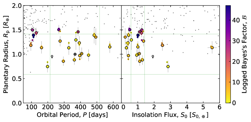
Figure 1: Our sample population of $\rm KOI$s (big colored circles with black outlines) and the remaining $\rm KOI$ background population (small black dots), distributed according to planetary radius, $R_{\rm p}$, orbital period, $P$ (left), and insolation flux, $S_{\rm 0}$ (right). Note that our sample uses the newly fitted/derived results of this work whereas background $\rm KOI$s draw from the preceding MCMC solutions of 2023_10_Lissauer. Our $\rm KOI$s are colored by their logged Bayes’s factor, $\mathcal{B}$—as recovered by the modelling of each individual $\rm KOI$ under $\rm PC$ (transit plus Gaussian process, $\rm TGP$) and $\rm FA$ (Gaussian process only, $\rm GP$) hypotheses—such that greater positive values indicate strong planet-candidacy and vice-versa for $\rm FA$s, while those near-zero can be interpreted as possessing inconclusive/weak significance either way (see § ​​ 2.1). The $\mathcal{B}$ values corresponding to our solutions are also used to outline associated 2023_10_Lissauer results (small black dots with colored outlines) in order to facilitate a visual comparison of the physical parameters recovered for each $\rm KOI$ analyzed by both studies. Green lines outline the range within which a $\rm KOI$ may be deemed sufficiently “Earth–Sun-like”; these are defined according to nominal Earth values for $R_{\rm p}$, and either $P$ or $S_{\rm 0}$ as $x\in\left[1\pm\left(\sqrt{2}-1\right)\right]x_{\boldsymbol{\rm\oplus}}$. Note that all $\rm KOI$s were also uniformly filtered by $R_{\rm\star}$ with respect to solar values according to these same bounds. We are complete in both boxes drawn by these lines. For ease of reference, Earth $\left(\boldsymbol{\rm\oplus}\right)$ and Venus $\left(\boldsymbol{\rm\venus}\right)$ are also plotted.

We describe our proposed methodology herein and apply it to select Kepler targets, including potential Earth–Sun and Venus–Sun analogs (see Figure 1). In § ​​ 2 we lay the statistical foundation for Bayesian model comparison, $\rm GP$s, and nested sampling (§ ​​ 2.1) before proceeding with the construction of our $\rm TGP$ and $\rm GP$ models (§ ​​ 2.2), an overview of the software architecture (§ ​​ 2.3), and ending with a summary of how we obtain derived parameters from fitted solutions (§ ​​ 2.4). We identify a sample population of small long-period low-$\rm S/N$ $\rm KOI$s—including Kepler’s most Earth–Sun-like exoplanet systems: Kepler-62f ($\rm KOI$-701.04; 2013_05_Borucki), Kepler-442b ($\rm KOI$-4742.01; 2015_02_Torres), and Kepler-452b ($\rm KOI$-7016.01; 2015_08_Jenkins)—whose preceding Markov Chain Monte-Carlo (MCMC; 1953_06_Metropolis; 1970_04_Hastings) solutions indicate potential for Earth–Sun and/or Venus–Sun analog candidacy in LABEL:sec:Candidates_Modelled_Herein. The subsections of LABEL:sec:Numerical_Results present and analyze $\rm TGP$ and $\rm GP$ UltraNest solutions relative to each other in the context of Bayesian evidences and potential biases. In LABEL:subsec:Strong_and_Weak_Cases, we interpret UltraNest solutions of Kepler-62f and $\rm KOI$-5227.01 to establish expected behavior from strong/weak $\rm PC$s. The widths of phased photometric data windows and priors have the potential to influence the recovered logged Bayes’s factor between models; the effects of this are explored throughout LABEL:subsec:Varying_Free_Parameters. This section is closed off by a comparison of the Bayesian evidence against the standard metrics of $\rm MES$ and $\rm S/N$ in LABEL:subsec:Comparisons_to_Multiple_Event_Statistic_and_Signal-to-Noise_Ratio. We conclude with a summary of this paper’s leading results in LABEL:sec:Conclusions and outline future work in LABEL:sec:Next_Steps. A list of terminology and acronyms can be found in LABEL:sec:Terminology_and_Acronyms.

2 Methodology

In this section, we introduce the reader to fundamental methodology upon which we base our analysis, beginning with a summary of Bayesian statistics and evidence-based model comparison in § ​​ 2.1. Our combined treatment of white and correlated noise by use of a Gaussian distribution and Matérn 3/2 kernel $\rm GP$ is established next. Following this, § ​​ 2.2 provides a breakdown of each model ($\rm TGP$ and $\rm GP$) in terms of their parameters. A step-by-step outline of our UltraNest software architecture and model fitting process for any given $\rm KOI$ can be read in § ​​ 2.3. Derived parameter calculations are detailed in § ​​ 2.4.

2.1 Model Comparison

Bayes’s theorem (1763_01_Bayes; 1774_Laplace)—which forms the basis of Bayesian statistics and probability theory—describes the process by which our knowledge of an event (posterior) is probabilistically updated according to existing information (prior) and new observations (likelihood). In other words, it allows us to adjust our understanding of the world in order to make better informed decisions/predictions. From a statistical perspective, we can model observed data, $\mathcal{D}$, via the inference of model parameters, $\theta$, using Bayes’s theorem:

$$\hyperlink{def:posteriors}{\mathcal{P_{D}}\left(\theta\right)}{}=\frac{\hyperlink{def:likelihood}{\mathcal{L_{D}}\left(\theta\right)}{}\hyperlink{def:priors}{\pi\left(\theta\right)}{}}{\hyperlink{def:evidence}{\mathcal{Z_{D}}}{}}\ ,$$ (1)

where the posteriors, $\mathcal{P_{D}}\left(\theta\right)$, are represented in terms of the likelihood, $\mathcal{L_{D}}\left(\theta\right)$, priors, $\pi\left(\theta\right)$, and Bayesian evidence (marginal likelihood integral), $\mathcal{Z_{D}}$. Here, $\mathcal{Z_{D}}$ gives the probability associated with observing this realization of $\mathcal{D}$ and is defined as:

$$\hyperlink{def:evidence}{\mathcal{Z_{D}}}{}\equiv\int\hyperlink{def:likelihood}{\mathcal{L_{D}}\left(\theta\right)}{}\hyperlink{def:priors}{\pi\left(\theta\right)}{}d\theta{}\ .$$ (2)

The $\mathcal{Z_{D}}$ encodes both $\mathcal{L_{D}}\left(\theta\right)$ and $\pi\left(\theta\right)$ information, so it is often employed as a metric of model suitability. Should one know the most suitable model for a given problem, the computationally expensive $\mathcal{Z_{D}}$ can be readily discarded in favor of obtaining only $\mathcal{P_{D}}\left(\theta\right)$ of modelled $\theta$ (e.g., likelihood-driven techniques such as MCMC). However, it is uncommon in real-world problems to possess the most suitable model with which $\mathcal{D}$ is described in totality. As such, $\mathcal{Z_{D}}$, and by extension the Bayes’s factor of any two models, $A$ and $B$,

$$\mathcal{B}_{A,B}\equiv\frac{\hyperlink{def:evidence}{\mathcal{Z_{D}}}{}_{,A}}{\hyperlink{def:evidence}{\mathcal{Z_{D}}}{}_{,B}}\ ,$$ (3)

play a crucial role in determining the most suitable model for $\mathcal{D}$. This statistically robust process of model selection is known as Bayesian model comparison (1939_Jeffreys; 1995_06_Kass; 2003_Mackay; 2020_07_Dunstan; 2022_01_Dunstan). Our study applies the logged form of the Bayes’s factor:

$$\log\left(\mathcal{B}_{A,B}\right)=\log\left(\hyperlink{def:evidence}{\mathcal{Z_{D}}}{}_{,A}\right)-\log\left(\hyperlink{def:evidence}{\mathcal{Z_{D}}}{}_{,B}\right)\ ;$$ (4)

this quantity is defined such that positive values favor model $A$ and negative values model $B$. We replace $A$ by the transit plus Gaussian process ($\rm TGP$; $\rm PC$ hypothesis) model and $B$ by the Gaussian process ($\rm GP$; $\rm FA$ hypothesis) model to obtain $\log\left(\mathcal{B}_{\rm TGP,GP}\right)$—whose notation we condense to $\mathcal{B}$:

$$\hyperlink{def:logB}{\mathcal{B}}{}\equiv\log\left(\mathcal{B}_{\rm TGP,GP}\right)\ .$$ (5)

Accordingly, increasingly positive values of $\mathcal{B}$ promote the existence of the transiting $\rm PC$ while their negative counterparts suggest a $\rm FA$ signal originating purely from noise. Values of $\mathcal{B}$ near zero indicate no statistically significant improvement given by the addition of transit parameters to the fit with respect to the null (noise) hypothesis; that is not to say that these are definitively $\rm PC$s or $\rm FA$s or that either fit is necessarily less robust, but that no statistically significant difference exists between hypotheses.

Given an informed choice of kernel (covariance function; see 2006_Rasmussen), a $\rm GP$ may target specific behavior or systematics within a given data set—this is particularly useful when attempting to fit correlated noise present in photometric time series observations. The Squared-Exponential (Radial Basis Function; 1966_Cheney; 1975_Davis; 1981_Powell) and Matérn (1960_Matern) kernel families have become popular for the treatment of systematics in astronomy (2012_01_Gibson; 2012_12_Roberts; 2015_02_Barclay; 2015_03_Aigrain; 2015_07_Evans; 2015_10_Czekala; 2016_07_Aigrain; 2017_04_Littlefair; 2017_12_Foreman_Mackey; 2018_02_Angus; 2019_03_Livingston; 2023_06_Brahm; 2023_08_Aigrain, etc.); while both are generally well-suited to smooth signal applications (e.g., stellar variability), the latter is also capable of handling rougher interference (e.g., sudden pixel sensitivity dropout as illustrated by Figure 19 of 2018_04_Thompson). Given the known characteristics of stellar and instrumental $\rm FA$ sources which contaminate Kepler photometry (2011_11_Gilliland; 2015_10_Gilliland; 2016_04_Van_Cleve; 2016_12_Van_Cleve; 2018_04_Thompson), we adopt the Matérn 3/2 kernel:

$$k\equiv\hyperlink{def:sigmac}{\sigma_{\rm c}}{}^{2}\left(1+\frac{\sqrt{3}\left|t-t^{\prime}\right|}{\hyperlink{def:lc}{l_{c}}{}}\right)\exp\left(-\frac{\sqrt{3}\left|t-t^{\prime}\right|}{\hyperlink{def:lc}{l_{c}}{}}\right)\ .$$ (6)

Here, $\sigma_{\rm c}$ and $l_{c}$ describe the amplitude and length scales of the correlated noise with which every pair of data points, $t$ and $t^{\prime}$, is conditioned. White noise is incorporated as a scaling factor to the error bars belonging to each photometric observation and is obtained by fitting the standard deviation, $\sigma_{\rm w}$, of a zero-mean Gaussian.

Nested sampling is a popular class of algorithm which approximates Equation 2 and provides posterior inference(s) as byproducts given $\mathcal{D}$, $\mathcal{L_{D}}\left(\theta\right)$, and $\pi\left(\theta\right)$. Our current infrastructure makes use of UltraNest, which requires user-defined $\mathcal{L_{D}}\left(\theta\right)$, and prior transforms or quantile functions mapping between physical parameter and unit hypercube sampling spaces. Uniform priors are used for all $\rm TGP$/$\rm GP$ parameters excluding limb-darkening parameters, $q_{\rm 1}$ and $q_{\rm 2}$, which instead use Gaussian priors (2013_11_Kipping).

2.2 Summary of Models

Table 1: Model Parameter Descriptions

Transit Model Parameters
$\bullet$ $\rho_{\rm\star}$: Mean stellar density $\left[\rm g\ cm^{-3}{}\right]$.
$\bullet$ $q_{\rm 1}$: 2013_11_Kipping limb-darkening [unitless].
$\bullet$ $q_{\rm 2}$: 2013_11_Kipping limb-darkening [unitless].
$\bullet$ $T_{\rm 0}$: Transit time series epicenter $\left[\rm days{}\right]$.
$\bullet$ $P$: Orbital period of the exoplanet $\left[\rm days{}\right]$.
$\bullet$ $b$: Impact parameter [unitless].
$\bullet$ $\hyperlink{def:Rp}{R_{\rm p}}{}/\hyperlink{def:Rstar}{R_{\rm\star}}{}$: Ratio of planetary and stellar radii [unitless].
$\bullet$ $F_{\rm 0}$: Relative photometric zero-point offset [unitless].
Noise Model Parameters
$\bullet$ $\sigma_{\rm w}$: Multiplicative factor applied to the photometric errors reported by DR25 (white noise) [unitless].
$\bullet$ $\sigma_{\rm c}$: Amplitude scale of Equation 6 [unitless].
$\bullet$ $l_{c}$: Length scale of Equation 6 [unitless].

Photometric exoplanet transits were modeled using transitfit5 (2016_08_Rowe). The lightcurve model uses the analytic limb-darkening transit from 2002_12_Mandel and assumes non-interacting Keplerian orbits. The model is parameterized with $\rho_{\rm\star}$, $q_{\rm 1}$, $q_{\rm 2}$, $T_{\rm 0}$, $P$, $b$, $\hyperlink{def:Rp}{R_{\rm p}}{}/\hyperlink{def:Rstar}{R_{\rm\star}}{}$, $F_{\rm 0}$, $\sqrt{\hyperlink{def:eccentricity}{e}{}}\cos\left(\hyperlink{def:wperi}{\omega}{}\right)$, $\sqrt{\hyperlink{def:eccentricity}{e}{}}\sin\left(\hyperlink{def:wperi}{\omega}{}\right)$, and a photometric dilution factor (see Table 1). The model can additionally include the effects of geometric albedo, ellipsoidal variations, and secondary eclipses. The calculation of Keplerian orbits derives the scaled semi-major axis, $a/\hyperlink{def:Rstar}{R_{\rm\star}}{}$, based on $\rho_{\rm\star}$; this calculation assumes that the planetary mass, $M_{\rm p}$, is much less than the mass of the host star, $M_{\rm\star}$. For all presented models in this paper, we assume: (1) circular orbits (i.e., zero eccentricity, $e$) such that $\hyperlink{def:ecosw}{\sqrt{\hyperlink{def:eccentricity}{e}{}}\cos\left(\hyperlink{def:wperi}{\omega}{}\right)}{}=\hyperlink{def:esinw}{\sqrt{\hyperlink{def:eccentricity}{e}{}}\sin\left(\hyperlink{def:wperi}{\omega}{}\right)}{}=0$, (2) no dilution (unresolved binaries), (3) no star-planet interactions, and (4) that the planet is completely dark (no reflection or emission). Limb-darkening parameters are from the tables of 2011_05_Claret for the Kepler bandpass. The shape information of low-$\rm S/N$ putative transit signatures within our regime of interest: (1) leaves $e$ and $\omega$ very weakly constrained and (2) makes uninformative limb-darkening priors superfluous. These assumptions and inputs to the modelling approach are similar to transit model results presented in DR25.

2.3 Software Architecture

The general step-by-step outline for the fitting of an individual $\rm KOI$ is detailed in this section.

1. Since the preceding MCMC architecture of 2023_10_Lissauer modelled the transit events of prewhitened data rather than simultaneously fitting correlated noise and transit events as performed in this study, we treat their transit solutions as initial guesses to define focused prior widths for our transit model in UltraNest; this mitigates computationally wasteful exploration of uninformative/unlikely parameter space.

2. For noise model hyperparameters, we define physically-motivated prior widths accordingly:

   1. While Kepler photometry typically falls within 10 – 20% of the predicted white noise budget (2011_11_Gilliland; 2015_10_Gilliland; 2016_04_Van_Cleve; 2016_12_Van_Cleve; 2018_04_Thompson), we err on the side of caution with a wide uninformative prior on the scaled photometric error of $\hyperlink{def:sigmaw}{\sigma_{\rm w}}{}\in\left[0.2,3.8\right]$.

   2. The amplitude scale of the correlated noise has prior width set as $\hyperlink{def:sigmac}{\sigma_{\rm c}}{}\in\left[0,\left(F_{max}-F_{min}\right)/2\right]$; this should not exceed the maximum flux semi-amplitude, $\left(F_{max}-F_{min}\right)/2$, observed in a given $\rm KOI$’s data set.

   3. The length scale of the correlated noise has prior width set as $\hyperlink{def:lc}{l_{c}}{}\in\left[2\Delta t{},2\hyperlink{def:sigmad}{\sigma_{\rm d}}{}\hyperlink{def:tT}{t_{\rm T}}{}\right]$; this should not fall below the measurement cadence, $\Delta t$, or exceed the phased photometric data window’s timescale, $2\hyperlink{def:sigmad}{\sigma_{\rm d}}{}\hyperlink{def:tT}{t_{\rm T}}{}$.

3. Define likelihood and prior cube transformation functions for UltraNest.

4. Set free parameters: $\sigma_{\rm d}$ and $\sigma_{\rm p}$.

5. Initialize and precompute all relevant values (i.e., $\rm GP$ kernel).

6. Conduct photometric time series data preprocessing/reduction, including the following:

   1. Removal of other threshold-crossing events ($\rm TCE$s)/$\rm KOI$s associated with the same host star.

   2. $\sigma_{\rm d}$ phased photometric data window width specification.

   3. Linear regression removal of ramps/slopes.

   4. Median-based zero-point correction.

   5. Removal of data $\pm 5\sigma$ beyond the MCMC data-residual median value to deal with uncorrected cosmic rays, flares, or uncorrected instrumental effects following 2018_04_Thompson.

7. Run UltraNest’s ReactiveNestedSampler with RegionSliceSampler enabled once per model ($\rm TGP$ and $\rm GP$).

To solve for the Matérn 3/2 $\rm GP$’s hyperparameters prior to each iteration’s likelihood evaluation, matrix inversion must be performed. Since the transit events are effectively isolated in time, their correlated noise components can be approximated to share negligible covariance; we represent this by means of a block-diagonal approximation to the kernel, drastically decreasing the computational burden of matrix inversions. Naturally, benefits in performance scale with the number of transit events in a given $\rm KOI$’s data set. For the task of inversion, we use Cholesky decomposition—a method roughly twice as efficient as lower-upper (LU) decomposition (1924_04_Cholesky; 1942_08_Banachiewicz; 1986_Press; 1995_04_Schwarzenberg_Czerny). Nonetheless, each iteration is still expensive.

2.4 Derived Parameters

Formulas for derived parameters can be found within this section. We compute transit duration according to Equation 16 of 2003_03_Seager, rewritten here using Kepler’s Third Law (1619_Kepler) as:

$$\hyperlink{def:tT}{t_{\rm T}}{}=\left(\frac{3\hyperlink{def:Period}{P}{}}{\pi^{2}G\hyperlink{def:rhostar}{\rho_{\rm\star}}{}}\right)^{\frac{1}{3}}\sqrt{\left(1+\frac{\hyperlink{def:Rp}{R_{\rm p}}{}}{\hyperlink{def:Rstar}{R_{\rm\star}}{}}\right)^{2}-\hyperlink{def:bimpact}{b}{}^{2}}.$$ (7)

The insolation flux, $\hyperlink{def:Szero}{S_{\rm 0}}{}\equiv L/4\pi a^{2}$, can be combined with Kepler’s Third Law to yield:

$$\frac{\text{<span class="ltx\_ref ltx\_font\_italic ltx\_ref\_self">S0</span>}}{\mathrm{S}{}_{0,\mathbf{\oplus }}}=\frac{L{}_{\star }}{\mathrm{L}{}_{\mathbf{\odot }}}\left[\frac{M{}_{\star }}{\mathrm{M}{}_{\mathbf{\odot }}}\right(\frac{\text{<span class="ltx\_ref ltx\_ref\_self">def:Period</span>}}{}$$ (8)