Modern nuclear and astrophysical constraints of dense matter in a renormalized chiral approach

Abstract

We explore the Quantum Chromodynamics (QCD) phase diagram’s complexities, including quark deconfinement transitions, liquid-gas phase changes, and critical points, using the chiral mean-field (CMF) model that is able to capture all these features. We introduce a vector meson renormalization within the CMF framework, enabling precise adjustments of meson masses and coupling strengths related to vector meson interactions. Performing a new fit to the deconfinement potential, we are able to replicate recent lattice QCD results, low energy nuclear physics properties, neutron star observational data, and key phase diagram features as per modern constraints. This approach enhances our understanding of vector mesons’ roles in mediating nuclear interactions and their impact on the equation of state, contributing to a more comprehensive understanding of the QCD phase diagram and its implications for nuclear and astrophysical phenomena.

I Introduction

Hot and/or dense Quantum Chromodynamics (QCD) matter is a fascinating area of research and its understanding requires knowledge of theoretical and experimental nuclear physics, astrophysics, particle physics, and gravity [1, 2, 3]. It includes the extreme conditions of temperature that existed shortly after the Big Bang, during the early moments of the universe’s formation. These conditions are believed to be reproduced in relativistic particle collisions, such as those created in high energy particle accelerators like the Large Hadron Collider (LHC) and the Relativistic Heavy-Ion Collider (RHIC) [4, 5]. On the other hand, QCD matter at effectively zero temperature (in the range of MeV) in neutron stars is another fascinating and complex area of study within nuclear astrophysics [6]. Neutron stars are incredibly dense celestial objects formed when massive stars undergo supernova explosions at the end of their life cycles. Significant interest is focused on trying to find exotic degrees of freedom like hyperons or deconfined quarks in the core of neutron stars [7, 8, 9], since this would be the only regime in the universe where they could be stable.

The QCD phase diagram delineates phases of strongly interacting matter, usually under varying temperature ($T$) and baryon chemical potential ($\mu_{B}$). At low $T$ and $\mu_{B}$, quarks and gluons are confined within hadrons (hadronic phase) and are expected to transition to an effective liberated state called deconfined quark matter at high $T$ and/or $\mu_{B}$  (see recent reviews [10, 11] from lattice QCD). In addition to the confinement/deconfinement quark hadron phase transition, there also exists a phase transition from nuclei to bulk hadronic matter known as liquid-gas phase transition at $T^{\rm LG}_{c}\simeq 15-17$ MeV($\mu^{\rm LG}_{B,c}\approx 910$ MeV) [12, 13, 14]. The QCD phase diagram is believed to encompass two critical points, the liquid-gas and hadron-quark. In both cases, the first-order phase transition coexistence lines are thought to stop at the respective critical points and become indistinct after that, which is referred to as a crossover regime (see Figure 1). Lattice QCD has proven to be highly effective for investigating strong interactions in the vicinity of and beyond the deconfinement phase transition zone within the QCD phase diagram in the high $T$ and low $\mu_{B}$ regime, primarily due to its ability to handle non-perturbative aspects [11]. Based on the latest lattice results, no sign of critical behavior has been found up to $\mu_{B}\approx 300$ MeV [15, 16], and the critical temperature is expected to be smaller than $T^{\rm HQ}_{c}=132^{+3}_{-6}$ MeV for isospin symmetric matter with zero baryon ($\mu_{B}$), charge ($\mu_{Q}$) and strange ($\mu_{S}$) chemical potential [17]. Within lattice QCD results, the crossover or pseudo-critical temperature (at $\mu_{B}$=0 axis) has been identified with extreme accuracy as $T^{p}_{c}=158\pm 0.6$ MeV [15], in addition to a first order deconfinement phase transition for pure gauge at a temperature of $T_{c}^{d}=$ 270 MeV [18]. On the other side of the diagram, in neutron stars, the critical density $n^{d}_{B,c}$, which marks the initial stage of the transition from hadronic matter to quark deconfinement is still not yet well constrained.

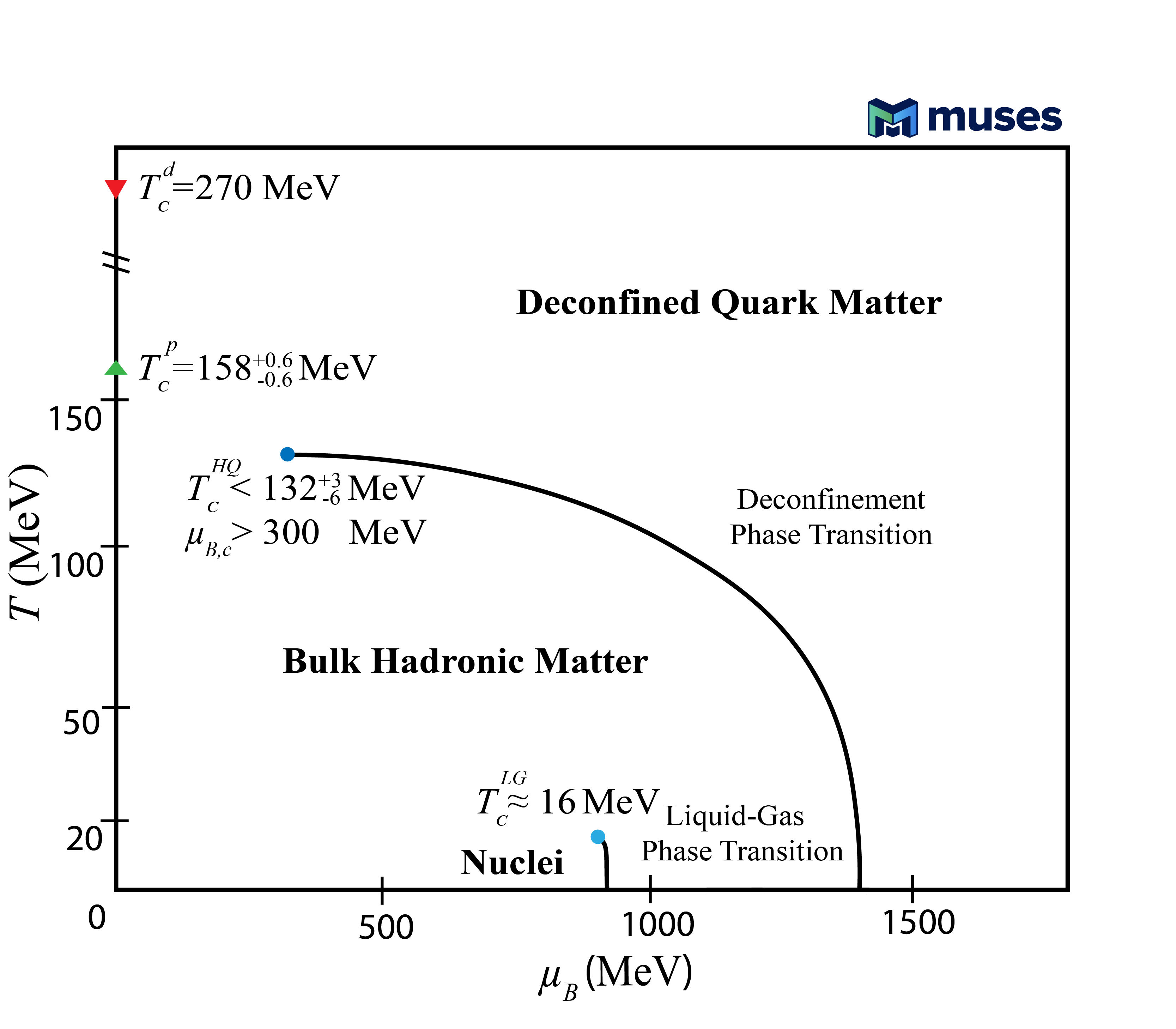
Figure 1: A rough sketch of the QCD phase diagram, including lattice QCD results and experimental data. $T^{d}_{c}$ and $T^{p}_{c}$ denote the deconfinement phase transition and pseudo critical phase transition respectively (both at $\mu_{B}=0$) while $\mu_{B,c}$ and $T^{HQ}_{c}$ represent the critical baryon chemical potential and critical temperature for hadron quark phase transition, and $T^{LG}_{c}$ the critical temperature for liquid-gas phase transition.

A core requirement for dense matter theories is the accurate reproduction of experimental data for isospin-symmetric nuclear matter at low temperature and around nuclear saturation density $n_{\mathrm{sat}}$. This entails crucial observables, such as the binding energy per nucleon $B/A$, compressibility $K$, symmetry energy $E_{\rm sym}$, and slope parameter $L$. Notably, recent progress has been made in the measurement of the parity-violating asymmetry term $A_{\mathrm{PV}}$ through elastic scattering of longitudinally polarized electrons on ²⁰⁸Pb. With this, the PREX collaboration’s findings have facilitated the determination of the nuclear saturation density value $n_{\mathrm{sat}}=0.1480\pm 0.0038~{}\mathrm{fm}^{-3}$ [19]. The binding energy per nucleon values were determined to be $B/A=$-15.677 MeV at a saturation density of $n_{\mathrm{sat}}$ = 0.16146 fm^-3 [20] and $B/A=$-16.24 MeV at $n_{\mathrm{sat}}$ = 0.16114 fm^-3 [21]. These values were obtained by analyzing experimental data from heavy nuclei masses and ground state masses of nuclei with neutron ($N$) and proton ($Z$) numbers greater than or equal to 8, respectively. The Isovector Giant Monopole Resonance (ISGMR) collective nucleon excitations from nuclei such as ⁹⁰Zr and ²⁰⁸Pb have suggested a value of $K=240\pm 20$ MeV for the incompressibility of infinite nuclear matter [22, 23, 24, 25]. But note that, in a comprehensive review [26], various methodologies and theories used between 1961 and 2016 led to a much larger range of $K$ values, from 100 MeV to 380 MeV, with relativistic mean-field models often predicting higher values. Finally, a range of $250<K<315$ MeV was obtained without assuming any specific microscopic model, except for the Coulomb effect [26].

Going further, the symmetry energy $E_{\rm sym}$ is the energy (per baryon) difference between nuclear matter with equal numbers of protons and neutrons (isospin-symmetric) and pure neutron matter. The slope parameter ($L$) is a measure of how rapidly $E_{\rm sym}$ (at $n_{\mathrm{sat}}$) changes with the baryon density. Both $E_{\rm sym}$ and $L$ are important quantities for understanding various nuclear phenomena, such as neutron star properties and low-energy heavy-ion collisions [27]. In Ref. [28], a comprehensive assessment based on 28 model evaluations utilized terrestrial nuclear experiments and astrophysical data to determine $E_{\rm sym}$ and $L$ at saturation density. Fiducial values emerged as $(31.6\pm 2.7)$ MeV for $E_{\rm sym}$ and $(58.9\pm 16)$ MeV for $L$. Extracting $E_{\rm sym}$ from experimental nuclear masses yielded $L=(50.0\pm 15.5)$ MeV at $n_{\mathrm{sat}}=0.16$ fm^-3 [29]. Interestingly, addressing ²⁰⁸Pb’s neutron skin thickness, PREX-II constrained the symmetry energy, revealing a large slope $L=(106\pm 37)$ MeV [30], consistently exceeding current bounds. On the other hand, another PREX-II study examined the parity-violating asymmetry $A_{\text{PV}}$ for ²⁰⁸Pb, leading to a neutron skin thickness $R^{208}_{\text{skin}}=(0.19\pm 0.02)$ fm and a much smaller value of slope $L=(54\pm 8)$ MeV [31], consistent with prior astrophysical estimates. Furthermore, the hyperon potential ($U_{H}$) describe the interactions between hyperons and nucleons at $n_{\rm{sat}}$ for isospin-symmetric matter. The $\Lambda$-nucleon potential, obtained from 1980s experiments, is firmly negative at around $U_{\Lambda}\sim-28$ MeV [32], with recent estimates clustering between $-32$ and $-30$ MeV [33]. The measurements from KEK Japan indicate a repulsive potential for $\Sigma$ ($U_{\Sigma}=30\pm 20$ MeV) and a joint collaboration between KEK and JPARC Japan give an attractive potential for $\Xi$ ($U_{\Xi}=-21.9\pm 0.7$ MeV) [34]. The ALICE collaboration’s p-$\Xi$ correlation functions report a less attractive potential of $U_{\Xi}=-4$ MeV, aligning with HAL-QCD collaboration’s (2+1)D lattice QCD calculations, yielding $U_{\Xi}=-4$ MeV, $U_{\Lambda}=-28$ MeV, and $U_{\Sigma}=+15$ MeV, with a statistical error of approximately $\pm 2$ MeV [35, 36, 37].

The nuclear matter characteristics exhibit significant correlations with macroscopic observables of neutron stars, such as the maximum mass ($M_{\rm max}$), radius $R_{M_{\rm max}}$, and tidal deformability ($\tilde{\Lambda}$). The determination of neutron star radii from NICER’s X-ray observations yield values of $12.39_{-1.98}^{+1.30}$ km for a $2.072_{-0.066}^{+0.067}$ solar mass ($M_{\odot}$)[38] and $13.7_{-1.5}^{+2.6}$ km for a $2.08_{-0.07}^{+0.07}$ $M_{\odot}$[39] neutron star, respectively. Additionally, the gravitational wave event GW170817, resulting from the merger of binary neutron stars (BNS), imposes a constraint on the tidal deformability, indicating $\tilde{\Lambda}<800$ for neutron stars with a mass of 1.4 solar masses [40]. A more detailed discussion about constraints from first principles, low energy nuclear experiments, heavy-ion experiments, and astrophysical observations is given in our recent review article [41].

Solving QCD analytically is a complex task, despite a well-defined Lagrangian. Lattice QCD represents space-time on a lattice where quarks and gluons reside at vertices, connected by gluon lines [42]. However, it’s limited by the sign problem at higher baryon chemical potentials [43, 44]. Perturbative QCD (pQCD) is applicable at large $\mu_{B}$ and/or $T$, but breaks down near the deconfinement phase transition due to large coupling constants [45, 46, 47]. At high temperature and low $\mu_{B}$, resummed pQCD calculations are in agreement with lattice data for $T\geq 250$ MeV [48, 49, 50]. Chiral effective theory ($\chi$EFT) is suitable at low densities and temperatures [51]. Despite these methods, the QCD phase diagram remains largely uncharted (see Figure 1 of Ref. [41]). That is where effective models come in, to bridge the gap between QCD complexities and first-principle limitations, providing valuable insights across a broad spectrum of QCD phenomena and constructing Lagrangians with the appropriate degrees of freedom [52, 53, 54]. In particular, relativistic chiral mean-field models can reproduce the restoration of chiral symmetry and quantify how hadronic masses are influenced by the medium [55, 56, 52, 57, 58].

From the latter class, non-linear chiral models stand out, based on a non-linear realization of chiral symmetry [56, 59, 60, 61, 62]. The introduction of a Polyakov-loop-inspired potential in a non-linear chiral model as a mechanism to deconfine quarks gave rise to the chiral mean-field (CMF) model [63]. Within the mean-field approximation, the CMF model agrees well with nuclear data [64]. It offers a unified description, allowing one to reproduce diverse scenarios, such as heavy-ion collisions and astrophysical phenomena, integrating quark deconfinement through an order parameter $\Phi$ with values dependent upon a Polyakov-like potential [65, 18]. The CMF model accommodates various temperatures, densities, and magnetic fields [66, 67, 68, 69, 70], enabling it to be used to explore various regions of QCD phase diagram [63, 71, 72, 73, 70]. However, these past works did not include a consistent treatment of mesons. The mesons lacked in-medium contributions and the vector-mesons masses were degenerate.

Understanding the importance of vector meson masses and interactions is a necessary step in the direction of incorporating thermal mesons in the formalism. In chiral models, hadronic masses are generated by interactions with the medium and can depend on $T$, $\mu_{B}$, etc. In relativistic mean-field models, vector interactions play a significant role in describing the behavior of hadrons and their connection within the framework of QCD. For example, vector mesons (such as the $\omega$ meson) couple to nucleons and interact with other hadrons, which further play a significant role in determining the stiffness of the equation of state (EoS) of nuclear matter in heavy-ion collisions and neutron stars. The role of vector mesons has been extensively studied in different theoretical approaches to determine properties of nuclear matter and compact stars [74, 75, 76, 77, 78, 79, 80, 81, 82, 83, 84, 85, 6, 86, 87, 88, 89, 90, 91, 92, 93, 94, 95, 96, 97, 98, 99, 100, 101, 102, 103, 104, 105, 106, 107, 108, 109, 94, 80, 110].

In the hadronic non-linear chiral model  [59, 111, 61, 64], vector mesons ($\omega$, $\rho$ and $\phi$) were also introduced as mediators of the strong interaction between nucleons and hyperons. The degenerate masses of different vector mesons ($\omega$, $\rho$, and $\phi$) were broken by introducing a renormalization of vector mesons through the utilization of proper invariants [59, 111]. For finite nuclei, the renormalization of vector mesons was used to break the mass degeneracy of $\omega$, $\phi$ and $K^{*}$ mesons [59]. In particular, in Ref. [111], utilizing a combination of two invariants, vector meson renormalization was employed to lift the mass degeneracy among $\omega$, $\phi$, and $\rho$ mesons. Note that, the renormalization of vector meson mean fields in chiral models involves adjusting parameters related to the coupling strengths or masses of the vector mesons to achieve a better match between the model predictions and experimental data. This is a complex and iterative process, often requiring sophisticated computational techniques and comparisons with experimental observables.

In this work, we employ vector meson renormalization to break the mass-degeneracy between the vector mesons in the CMF model for the first time. We re-fit the vector meson coupling strengths to nucleons such as $g_{N\omega}$, $g_{N\rho}$ and $g_{4}$ (the coupling strength related to the effective self-interactive vector Lagrangian) to the saturation properties of the nuclear matter. The addition of a vector meson renormalization then significantly affects other properties within the CMF model, such that we need to re-parameterize other parameters that we detail here. These changes then require that we must re-fit the coupling constants related to the Polyakov-like potential within the CMF model to reproduce recent lattice data. We also incorporate updated information about the phase diagram that has changed since the last time the finite temperature CMF model parameters were parameterized (in 2008). The changes include state-of-the-art and updated information about the deconfinement phase transition, pseudo-critical temperature, liquid-gas critical point, deconfinement critical point, and observational data for neutron stars. Note that the renormalized vector meson fields significantly affect the in-medium properties of vector mesons, which will be studied in a future work.

The outline of this paper is as follows. In Section II.1, the details of the CMF model are given along with the Polyakov-like potential. In Section II.2, a detailed derivation of renormalized vector-meson mean fields is provided and the same is applied for different self-interactions of vector mesons. In Section III, the results are presented for each part of QCD phase diagram. Finally, we present a summary with discussions in Section IV.

II Formalism

II.1 Chiral mean-field model

In this work, we build on the CMF model, which incorporates fundamental QCD aspects like the trace anomaly, spontaneous breaking of chiral symmetry and deconfinement [56, 112]. Based on a non-linear realization of chiral symmetry, this framework employs scalar and vector fields to describe meson-baryon/quark interactions. The scalar-isoscalar field $\sigma$ corresponds loosely to the light quark composed meson $\sigma_{0}(500)(u\bar{d})$. A strange scalar-isoscalar field $\zeta$ is linked to the strange quark-containing meson $s\bar{s}$, crucial to describe strange matter [113]. Additionally, the scalar-isovector field $\delta$ addresses isospin asymmetric matter and introduces mass splitting between isospin multiplet and being associated with the meson $(\bar{u}u-\bar{d}d)$ [114, 115]. These fields mediate interactions among nucleons, hyperons, and quarks, contributing to attractive medium-range forces (scalar fields) and short-range repulsion (vector fields, e.g., vector-isoscalar $\omega$, strange vector-isoscalar $\phi$, and vector-isovector $\rho$) depending on $T,\mu_{B}$, etc. The scalar dilaton field, $\chi$, representing the hypothetical glueball field, is introduced to replicate QCD’s trace anomaly [59]. Nevertheless, due to the little overall contribution of $\chi$ field to baryon thermodynamic quantities, we use the so-called frozen glueball approximation ($\chi=\chi_{0}$), where $\chi_{0}$ is the vacuum value of the dilaton field.

The mean field approximation (MFA) involves replacing the meson fields with their respective expectation values, effectively treating them as classical fields. As a result, only mesons along the diagonal of the scalar meson matrix $X$ (Eq. 30) have non-zero values due to the preservation of parity. Furthermore, all scalar and vector mesons are simplified into constants that are independent of both time and space. As a result of this approximation, the mean-field CMF Lagrangian reads [63]

$$\mathcal{L}_{\rm CMF}=\mathcal{L}_{\rm kin}+\mathcal{L}_{\rm int}+\mathcal{L}_{\rm scal}+\mathcal{L}_{\rm vec}+\mathcal{L}_{\rm SB}-U_{\Phi}\,.$$ (1)

Above, ${\cal L}_{\rm kin}$ stands for the kinetic energy of spin-1/2 fermions (octet baryons + quarks), ${\cal L}_{\rm int}$ represents interactions of spin-1/2 fermions with vector and scalar mesons, ${\cal L}_{\rm scal}$ stands for the self-interactions of scalar mesons, while ${\cal L}_{\rm vec}$ contributes to vector meson masses and includes quartic self-interaction terms (see Section II.2 for details). ${\cal L}_{\rm SB}$ denotes an explicit chiral symmetry breaking contribution. The second term in ${\cal L}_{\rm SB}$ (see below) allows the CMF model to reproduce the experimental values of hyperon potentials. Explicitly, these terms can be written as

$$\mathcal{L}_{\rm kin} =\sum_{i\,\in\,fermions}\bigg{[}\bar{\psi}_{i}i\gamma_{\mu}\partial^{\mu}\psi_{i}\bigg{]},$$

$$\mathcal{L}_{\rm int} =-\sum_{i\in fermions}\bar{\psi}_{i}\big{[}\gamma_{0}\big{(}g_{i\omega}\omega+g_{i\rho}\rho+g_{i\phi}\phi\big{)}+m_{i}^{*}\big{]}\psi_{i}\,,$$

$$\mathcal{L}_{\rm scal} =-\frac{1}{2}k_{0}\chi_{0}^{2}(\sigma^{2}+\zeta^{2}+\delta^{2})+k_{1}(\sigma^{2}+\zeta^{2}+\delta^{2})^{2}$$

$$+k_{2}\left[\frac{\sigma^{4}+\delta^{4}}{2}+\zeta^{4}+3\left(\sigma\delta\right)^{2}\right]+k_{3}\chi_{0}\left(\sigma^{2}-\delta^{2}\right)\zeta$$

$$-k_{4}\chi_{0}^{4}+\frac{\epsilon}{3}\chi_{0}^{4}\ln\left[\frac{\left(\sigma^{2}-\delta^{2}\right)\zeta}{\sigma_{0}^{2}\zeta_{0}}\right],$$

$$\mathcal{L}_{\rm vec} =\quad\mathrm{discussed}\ \mathrm{in}\ \mathrm{\lx@cref{creftype~refnum}{sec:Lag_vec_ren}},$$

$$\mathcal{L}_{\rm SB} =-\left[m_{\pi}^{2}f_{\pi}\sigma+\left(\sqrt{2}m_{K}^{2}f_{K}-\frac{1}{\sqrt{2}}m_{\pi}^{2}f_{\pi}\right)\zeta\right]$$

$$-m_{3}\sum_{i\,\in\,hyperons}\bigg{[}\bar{\psi}_{i}\left(\sqrt{2}(\sigma-\sigma_{0})+(\zeta-\zeta_{0})\right)\psi_{i}\bigg{]},$$ (2)

where $\psi$ represents the fermionic field, $g^{\prime}s$ denote the corresponding coupling constants of fermions with meson mean-fields, $k^{\prime}s$ are the fitting parameters associated with the scalar mesons, and $\epsilon$ is a model parameter related to the QCD trace anomaly. The variables: $m_{K}$, $m_{\pi}$, $f_{K}$, and $f_{\pi}$ are the masses and decay constants of the kaons and pions, respectively. The parameter $m_{3}$ is associated with the explicit chiral symmetry breaking and is fitted to reproduce hyperon potentials.

The expansion of the mean field hadronic chiral non-linear model into quark degrees of freedom (CMF model) shares similarities with the Polyakov-loop-extended Nambu-Jona-Lasinio (PNJL) model [116]. The CMF utilizes a scalar field $\Phi$, analogous to the PNJL, to suppress quark degrees of freedom at low densities and/or temperatures. In our context, $\Phi$ is the scalar field associated with the PNJL-like effective potential that drives the transition from confined to deconfined phases. This transition is phenomenologically captured by the order parameter $\Phi\in[0,1]$. The modification of Polyakov potential from its original PNJL model form [116, 18] includes the incorporation of terms dependent on the baryon chemical potential. This adaptation enables the exploration of low-temperature and high-density scenarios, such as those encountered in neutron stars. The deconfinement potential in the CMF model reads [63]

$$U_{\Phi} =\left(a_{0}T^{4}+a_{1}\mu_{B}^{4}+a_{2}T^{2}\mu_{B}^{2}\right)\Phi^{2}$$

$$+a_{3}T_{0}^{4}\ln\left(1-6\Phi^{2}+8\Phi^{3}-3\Phi^{4}\right),$$ (3)

where the $a$’s and $T_{0}$ are parameters fitted to the known constraints of QCD phase diagram at higher temperatures and are discussed in Section III.2.

The presence of the scalar field $\Phi$ is introduced as an additional contribution to the effective masses of the baryons

$$m_{i}^{*} =g_{i\sigma}\sigma+g_{i\zeta}\zeta+g_{i\delta}\delta+\Delta m_{i}+g_{i\Phi}\Phi^{2},$$ (4)

and quarks

$$m_{i}^{*} =g_{i\sigma}\sigma+g_{i\zeta}\zeta+g_{i\delta}\delta+\Delta m_{i}+g_{i\Phi}\left(1-\Phi\right).$$ (5)

In the above equations, $\Phi\sim 0$ denotes a system dominated by hadrons, $\Phi\sim 1$ represents a quark-dominated state, and intermediate values indicate a coexistence of hadrons and deconfined quarks (relevant only at high temperatures). Moreover, in those equations, the $g^{\prime}s$ are the corresponding coupling constants of fermions with the scalar fields. Note that the parameter $\Delta m_{i}$ incorporates effects from additional sources, such as the Higgs field $m^{q}_{0}$ (pertaining to quarks), bare mass $m_{0}$ (for octet baryons) and explicit symmetry breaking term $m_{3}$ (relevant to hyperons)

$$\Delta m_{N} =m_{0}\,,$$

$$\Delta m_{\Lambda} =m_{0}-m_{3}\left(\sqrt{2}\sigma_{0}+\zeta_{0}\right),$$

$$\Delta m_{\Sigma} =m_{0}-m_{3}\left(\sqrt{2}\sigma_{0}+\zeta_{0}\right),$$

$$\Delta m_{\Xi} =m_{0}-m_{3}\left(\sqrt{2}\sigma_{0}+\zeta_{0}\right),$$

$$\Delta m_{u} =\Delta m_{d}=m_{0}^{u}\,,\quad\Delta m_{s}=m_{0}^{s}\,.$$ (6)

The coupling constants $g^{\prime}s$ between baryons and scalar mesons are fitted in order to obtain correct vacuum masses of the baryons in vacuum. The other parameters ($k$’s and $\epsilon$), related to scalar interactions, are computed in order to obtain correct vacuum expectation values for the $\sigma$, $\zeta$, and $\chi$ field equations and to reproduce $\sigma$, $\eta$, and $\eta^{\prime}$ vacuum masses [63]. In Table 1, a list of CMF parameters associated with baryons is tabulated, whereas Table 2 reflects the CMF parameters related to quark sector (the only ones we do not modify in this work). The quark scalar couplings are fixed as approximately one third of nucleon scalar couplings, whereas vector couplings are set to zero as suggested by Ref. [117]. In the next section, we discuss the vector meson interaction Lagrangian ${\cal L}_{\rm vec}$ in detail.

Table 1: Parameters related to the scalar interaction for baryons.

$\sigma_{0}=-93.3$ MeV	$\delta_{0}=0$	$\zeta_{0}=-106.56$ MeV
$g_{N\sigma}=-9.83$	$g_{N\delta}=-2.34$	$g_{N\zeta}=1.22$
$g_{\Lambda\sigma}=-5.52$	$g_{\Lambda\delta}=0$	$g_{\Lambda\zeta}=-2.3$
$g_{\Sigma\sigma}=-4.01$	$g_{\Sigma\delta}=-6.95$	$g_{\Sigma\zeta}=-4.44$
$g_{\Xi\sigma}=-1.67$	$g_{\Xi\delta}=-4.61$	$g_{\Xi\zeta}=-7.75$
$k_{0}=2.37$	$k_{1}=1.40$	$k_{2}=-5.55$
$k_{3}=-2.65$	$\chi_{0}=401.93$ MeV	$\epsilon=2/33$
$m_{3}=0.8061$

Table 2: Parameters related to the scalar and vector interaction for quarks.

$g_{q\omega}=0$	$g_{q\phi}=0$	$g_{q\rho}=0$
$g_{q\sigma}=-3$	$g_{q\delta}=0$	$g_{q\zeta}=-3$
$m^{u}_{0}=5$ MeV	$m^{d}_{0}=5$ MeV	$m^{s}_{0}=150$ MeV

II.2 Renormalization of the Lagrangian

II.2.1 Kinetic and mass terms for vector mesons

We start with the simplest scale invariant mass term of renormalized vector interaction Lagrangian denoted by “tildes”

$$\mathcal{\tilde{L}}_{\rm vec}^{m}=\frac{1}{2}m_{V}^{2}\operatorname{Tr}\tilde{V}_{\mu}\tilde{V}^{\mu},$$ (7)

where $\tilde{V}_{\mu}$ is the degenerate renormalized vector meson matrix given by Eq. 32. Simplifying,

$$\mathcal{\tilde{L}}_{\rm vec}^{m}=m^{2}_{V}\left(\frac{\tilde{\omega}^{2}}{2}+\frac{\tilde{\phi}^{2}}{2}+\frac{3\tilde{\rho}^{2}}{2}+2\tilde{K}^{*}{{}^{2}}\right),$$ (8)

dividing the $\rho$ and $K^{*}$ terms by the degeneracy factor 3 and 4, respectively, we obtain

$$\mathcal{\tilde{L}}_{\rm vec}^{\rm m}=\frac{1}{2}m^{2}_{V}\left(\tilde{\omega}^{2}+\tilde{\phi}^{2}+\tilde{\rho}^{2}+\tilde{K}^{*}{{}^{2}}\right).$$ (9)

The equation above suggests that the vector meson nonet is mass degenerate. To correct that and split the masses, one can add the chiral invariant (CI) [59]

$$\mathcal{\tilde{L}}_{\rm vec}^{\rm CI}=\frac{1}{4}\mu\operatorname{Tr}\left[\tilde{V}_{\mu\nu}\tilde{V}^{\mu\nu}\left\langle X\right\rangle^{2}\right],$$ (10)

where $\left\langle X\right\rangle$ is the scalar meson matrix in the mean-field approximation given by Eq. 30 (for simplicity, we have taken vacuum values of the scalar meson fields), ${V}_{\mu\nu}$ is the renormalized vector meson tensor matrix given by Eq. 33 and $\mu$ is a parameter. In Ref. [118], an additional invariant term, $\left(\operatorname{Tr}V_{\mu\nu}\right)^{2}$, was incorporated into the expression presented in Eq. (10) to lift the mass degeneracy between the $\rho$ and $\omega$ mesons; however this provides a small correction and does not offer an explanation for the vector Kaon masses. Since the process of renormalizing the vector Kaons is a crucial initial step, laying the groundwork for future work beyond mean-field theory, we focus on Eq. 10.

Expanding it gives

$$\mathcal{\tilde{L}}_{\rm vec}^{\rm CI}= \frac{1}{4}\mu\Bigg{(}\frac{\sigma_{0}^{2}}{2}(\tilde{V}^{\mu\nu}_{\omega})^{2}+3\frac{\sigma_{0}^{2}}{2}(\tilde{V}^{\mu\nu}_{\rho})^{2}+(\tilde{V}^{\mu\nu}_{\phi})^{2}\zeta_{0}^{2}$$

$$+(\tilde{V}^{\mu\nu}_{K^{*}})^{2}(\sigma_{0}^{2}+2\zeta_{0}^{2})\Bigg{)}.$$ (11)

Dividing the $\rho$ term by 3 and the $K^{*}$ term by 4 based on their respective degeneracies, we obtain,

$$\mathcal{\tilde{L}}_{\rm vec}^{\rm CI}= \frac{1}{4}\mu\Bigg{(}\frac{\sigma_{0}^{2}}{2}(\tilde{V}^{\mu\nu}_{\omega})^{2}+\frac{\sigma_{0}^{2}}{2}(\tilde{V}^{\mu\nu}_{\rho})^{2}+(\tilde{V}^{\mu\nu}_{\phi})^{2}\zeta_{0}^{2}$$

$$+\frac{(\tilde{V}^{\mu\nu}_{K^{*}})^{2}}{2}\left(\frac{\sigma_{0}^{2}}{2}+\zeta_{0}^{2}\right)\Bigg{)}.$$ (12)

The kinetic energy vector term $\mathcal{L}_{\rm vec}^{\rm kin}=-\frac{1}{4}\operatorname{Tr}\left({V}_{\mu\nu}{V}^{\mu\nu}\right)$ when renormalized becomes

$$\mathcal{\tilde{L}}_{\rm vec}^{\rm kin} =-\frac{1}{4}\operatorname{Tr}\left(\tilde{V}_{\mu\nu}\tilde{V}^{\mu\nu}\right),$$

$$=-\frac{1}{4}\left(\left(\tilde{V}_{\rho}^{\mu\nu}\right)^{2}+\left(\tilde{V}_{K^{*}}^{\mu\nu}\right)^{2}+\left(\tilde{V}_{\omega}^{\mu\nu}\right)^{2}+\left(\tilde{V}_{\phi}^{\mu\nu}\right)^{2}\right).$$ (13)

Now, combining the contributions from Eq. 10 with Eq. 13 and identifying them to the non-renormalized kinetic energy term

$$\mathcal{L}_{\rm vec}^{\rm kin} =\mathcal{\tilde{L}}_{\rm vec}^{\rm kin}+\mathcal{\tilde{L}}_{\rm vec}^{\rm CI},$$

$$=-\frac{1}{4}\left[1-\mu\frac{\sigma_{0}^{2}}{2}\right]\left(\tilde{V}_{\tilde{\rho}}^{\mu\nu}\right)^{2}-\frac{1}{4}\left[1-\mu\frac{\sigma_{0}^{2}}{2}\right]\left(\tilde{V}_{\tilde{\omega}}^{\mu\nu}\right)^{2}$$

$$\quad-\frac{1}{4}\left[1-\frac{1}{2}\mu\left(\frac{\sigma_{0}^{2}}{2}+\zeta_{0}^{2}\right)\right]\left(\tilde{V}_{\tilde{K}^{*}}^{\mu\nu}\right)^{2}$$

$$\quad-\frac{1}{4}\left[1-\mu\zeta_{0}^{2}\right]\left(\tilde{V}_{\tilde{\phi}}^{\mu\nu}\right)^{2},$$

$$=-\frac{1}{4}Z_{\rho}^{-1}\left(\tilde{V}_{\tilde{\rho}}^{\mu\nu}\right)^{2}--\frac{1}{4}Z_{\omega}^{-1}\left(\tilde{V}_{\tilde{\omega}}^{\mu\nu}\right)^{2}$$

$$\quad-\frac{1}{4}Z_{K^{*}}^{-1}\left(\tilde{V}_{\tilde{K^{*}}}^{\mu\nu}\right)^{2}-\frac{1}{4}Z_{\phi}^{-1}\left(\tilde{V}_{\tilde{\phi}}^{\mu\nu}\right)^{2},$$ (14)

we obtain

$$\tilde{V}_{{\xi}}^{\mu\nu}=\partial^{\mu}\tilde{\xi}^{\nu}-\partial^{\nu}{\tilde{\xi}}^{\mu} =Z_{\xi}^{1/2}(\partial^{\mu}{\xi}^{\nu}-\partial^{\nu}{\xi}^{\mu})=Z_{\xi}^{1/2}{V}_{{\xi}}^{\mu\nu},$$

$$\mathrm{and}\quad\quad\quad\quad\quad\xi =Z_{\xi}^{-1/2}\tilde{\xi}\,,$$ (15)

where $\xi=\rho,\omega,K^{*},\phi$. Explicitly, the renormalization constants are given as

$$Z_{\rho}^{-1}=Z_{\omega}^{-1}=\left(1-\mu\frac{\sigma_{0}^{2}}{2}\right),\quad Z_{\phi}^{-1}=\left(1-\mu\zeta_{0}^{2}\right),$$

$$Z_{K^{*}}^{-1}=\left(1-\frac{1}{2}\mu\left(\frac{\sigma_{0}^{2}}{2}+\zeta_{0}^{2}\right)\right).$$ (16)

The net Lagrangian for the vector meson fields (with implicit renormalized contribution) is evaluated by adding Eqs. 9 and 14 using Eq. 15

$$\mathcal{L}_{\rm vec} =\mathcal{L}_{\rm vec}^{\rm kin}+\mathcal{L}_{\rm vec}^{\rm m},$$

$$=-\frac{1}{4}\left(\left(V_{\rho}^{\mu\nu}\right)^{2}+\left(V_{K^{*}}^{\mu\nu}\right)^{2}+\left(V_{\omega}^{\mu\nu}\right)^{2}+\left(V_{\phi}^{\mu\nu}\right)^{2}\right)$$

$$\quad+\frac{1}{2}\left(m_{\rho}^{2}\rho^{2}+m^{2}_{K^{*}}K{{}^{*}}^{2}+m_{\omega}^{2}\omega^{2}+m_{\phi}^{2}\phi^{2}\right),$$ (17)

where

$$m_{K^{*}}^{2}=Z_{K^{*}}m_{V}^{2},~{}~{}m_{\omega/\rho}^{2}=Z_{\omega/\rho}m_{V}^{2},~{}~{}m_{\phi}^{2}=Z_{\phi}m_{V}^{2},$$ (18)

denote the respective vector meson masses in the vacuum. The parameters, $m_{V}=687.33$ MeV and $\mu=$ $0.41/\sigma_{0}^{2}$ are fitted to obtain the correct $\omega,\phi$, $\rho$, and $K^{*}$ masses that are tabulated in Table 3, together with the old unrenormalized mass.

Table 3: Vacuum masses of vector mesons before (old) and after (new) employing the renormalization.

Meson	$\omega$	$\rho$	$K^{*}$	$\phi$
Old Mass (MeV)	687.33	687.33	687.33	687.33
New Mass (MeV)	770.87	770.87	865.89	1007.76

II.2.2 Self-interaction term for vector mesons

We start by adding a self-interactive Lagrangian term to Eq. 17

$$\mathcal{L}_{\rm vec} =\mathcal{L}_{\rm vec}^{\rm kin}+\mathcal{L}_{\rm vec}^{\rm m}+\mathcal{L}_{\rm vec}^{\rm SI}\,.$$ (19)

The different possible self-interaction (SI) terms of the vector mesons that are chiral invariant [99] can be written as the following coupling schemes: (shown here in renormalized version for the first time)

$$\text{ ${}^{\mathrm{R}}$C1: }\mathcal{\tilde{L}}_{\rm vec}^{\rm SI}=2\tilde{g}_{4}\operatorname{Tr}\left(\tilde{V}^{4}\right),$$ (20)

$$\text{ ${}^{\mathrm{R}}$C2: }\mathcal{\tilde{L}}_{\rm vec}^{\rm SI}=\tilde{g}_{4}\Bigg{[}\frac{3}{2}\left[\operatorname{Tr}\left(\tilde{V}^{2}\right)\right]^{2}-\operatorname{Tr}\left(\tilde{V}^{4}\right)\Bigg{]},$$ (21)

$$\text{ ${}^{\mathrm{R}}$C3: }\mathcal{\tilde{L}}_{\rm vec}^{\rm SI}=\tilde{g}_{4}\left[\operatorname{Tr}\left(\tilde{V}^{2}\right)\right]^{2},$$ (22)

$$\text{ ${}^{\mathrm{R}}$C4: }\mathcal{\tilde{L}}_{\rm vec}^{\rm SI}=\tilde{g}_{4}\frac{[\operatorname{Tr}(\tilde{V})]^{4}}{4}\,,$$ (23)

where superscript “R” denotes the renormalized coupling scheme. The coupling scheme C2, is a linear combination of C1 and C3 and is constructed in order to eliminate the $\omega\rho$ mixing term.

Now, after substituting the matrix $V$ (Eq. 32) in the above equations and simplifying them, we obtain the following equations

• ^RC1:

  $$\mathcal{\tilde{L}}_{\rm vec}^{\rm SI}=\tilde{g}_{4}\left(\tilde{\omega}^{4}+6\tilde{\omega}^{2}\tilde{\rho}^{2}+\tilde{\rho}^{4}+2\tilde{\phi}^{4}\right),$$

  $$\mathcal{L}_{\rm vec}^{\rm SI} =\frac{g_{4}}{Z_{\omega}^{2}}\left(Z_{\omega}^{2}\omega^{4}+6Z_{\omega}Z_{\rho}\omega^{2}\rho^{2}+Z^{2}_{\rho}\rho^{4}+2Z_{\phi}^{2}\phi^{4}\right)=g_{4}\left(\omega^{4}+6\frac{Z_{\rho}}{Z_{\omega}}\omega^{2}\rho^{2}+\left(\frac{Z_{\rho}}{Z_{\omega}}\right)^{2}\rho^{4}+2\left(\frac{Z_{\phi}}{Z_{\omega}}\right)^{2}\phi^{4}\right).$$ (24)

• ^RC2:

  $$\mathcal{\tilde{L}}_{\rm vec}^{\rm SI}=\tilde{g}_{4}\left(\tilde{\omega}^{4}+\tilde{\rho}^{4}+\frac{\tilde{\phi}^{4}}{2}+3\tilde{\rho}^{2}\tilde{\phi}^{2}++3\tilde{\omega}^{2}\tilde{\phi}^{2}\right),$$

  $$\mathcal{L}_{\rm vec}^{\rm SI} =\frac{g_{4}}{Z^{2}_{\omega}}\left(Z^{2}_{\omega}\omega^{4}+Z^{2}_{\rho}\rho^{4}+Z^{2}_{\phi}\frac{\phi^{4}}{2}+3Z_{\rho}Z_{\phi}\rho^{2}\phi^{2}+3Z_{\omega}Z_{\phi}\omega^{2}\phi^{2}\right),$$

  $$=g_{4}\left(\omega^{4}+\left(\frac{Z_{\rho}}{{Z_{\omega}}}\right)^{2}\rho^{4}+\left(\frac{Z_{\phi}}{{Z_{\omega}}}\right)^{2}\frac{\phi^{4}}{2}+3\left(\frac{Z_{\rho}}{{Z_{\omega}}}\frac{Z_{\phi}}{{Z_{\omega}}}\right)\rho^{2}\phi^{2}+3\left(\frac{Z_{\phi}}{{Z_{\omega}}}\right)\omega^{2}\phi^{2}\right).$$ (25)

• ^RC3:

  $$\mathcal{\tilde{L}}_{\rm vec}^{\rm SI}=g_{4}\left(\tilde{\omega}^{4}+2\tilde{\omega}^{2}\tilde{\rho}^{2}+\tilde{\rho}^{4}+2\tilde{\omega}^{2}\tilde{\phi}^{2}+\tilde{\phi}^{4}+2\tilde{\rho}^{2}\tilde{\phi}^{2}\right),$$

  $$\mathcal{L}_{\rm vec}^{\rm SI} =\frac{g_{4}}{Z^{2}_{\omega}}\left(Z^{2}_{\omega}\omega^{4}+2Z_{\omega}Z_{\rho}\omega^{2}\rho^{2}+Z^{2}_{\rho}\rho^{4}+2Z_{\omega}Z_{\phi}\omega^{2}\phi^{2}+Z^{2}_{\phi}\phi^{4}+2Z_{\phi}Z_{\rho}\rho^{2}\phi^{2}\right),$$

  $$=g_{4}\left(\omega^{4}+2\frac{Z_{\rho}}{Z_{\omega}}\omega^{2}\rho^{2}+\left(\frac{Z_{\rho}}{Z_{\omega}}\right)^{2}\rho^{4}+2\frac{Z_{\phi}}{Z_{\omega}}\omega^{2}\phi^{2}+\left(\frac{Z_{\phi}}{Z_{\omega}}\right)^{2}\phi^{4}+2\left(\frac{Z_{\rho}}{{Z_{\omega}}}\frac{Z_{\phi}}{{Z_{\omega}}}\right)\rho^{2}\phi^{2}\right).$$ (26)

• ^RC4:

  $$\mathcal{\tilde{L}}_{\rm vec}^{\rm SI}=\tilde{g}_{4}\left(\tilde{\omega}^{4}+2\sqrt{2}\tilde{\omega}^{3}\tilde{\phi}+3\tilde{\omega}^{2}\tilde{\phi}^{2}+\sqrt{2}\tilde{\omega}\tilde{\phi}^{3}+\frac{\tilde{\phi}^{4}}{4}\right),$$

  $$\mathcal{L}_{\rm vec}^{\rm SI} =\frac{g_{4}}{Z_{\omega}^{2}}\left(Z_{\omega}^{2}\omega^{4}+2\sqrt{2}Z_{\omega}^{3/2}\omega^{3}Z_{\phi}^{1/2}\phi+3Z_{\omega}\omega^{2}Z_{\phi}\phi^{2}+\sqrt{2}Z_{\omega}^{1/2}\omega Z_{\phi}^{3/2}\phi^{3}+\frac{Z_{\phi}^{2}\phi^{4}}{4}\right),$$

  $$=g_{4}\left(\omega^{4}+2\sqrt{2}\bigg{(}\frac{Z_{\phi}}{Z_{\omega}}\bigg{)}^{1/2}\omega^{3}\phi+3\bigg{(}\frac{Z_{\phi}}{Z_{\omega}}\bigg{)}\omega^{2}\phi^{2}+\sqrt{2}\bigg{(}\frac{Z_{\phi}}{Z_{\omega}}\bigg{)}^{3/2}\omega\phi^{3}+\frac{1}{4}\bigg{(}\frac{Z_{\phi}}{Z_{\omega}}\bigg{)}^{2}\phi^{4}\right),$$ (27)

which are obtained using the renormalized expressions of the fields in Eq. 15 and defining a coupling constant $g_{4}=Z^{2}_{\omega}\tilde{g}_{4}$.

The vector coupling constants $g_{N\omega}$, $g_{N\rho}$, and $g_{4}$ are adjusted to match nuclear saturation properties, as explained in Section III.1. Additionally, it is worth noting that the couplings involving interactions between nucleons and $\omega$ mesons, as well as nucleons and $\rho$ mesons, are influenced by the field redefinitions, leading to corresponding renormalized coupling constants: $g_{N\omega}\equiv 3g_{V}^{8}\sqrt{Z_{\omega}}$ and $g_{N\rho}\equiv g_{V}^{8}\sqrt{Z_{\rho}}$ [111]. Furthermore, it is important to highlight that the coupling scheme labeled as ^RC4 has a unique characteristic, involving contributions that exhibit linearity with respect to the isoscalar vector field $\phi$, leading to significant changes in the model’s behavior that help to reproduce astrophysical data, such as 2$M_{\odot}$ neutron stars.

III Results and Discussions

In this section, we present our numerical findings concerning the vector mesons, their masses and the deconfinement potential in the CMF model. These parameters have been adjusted to accurately replicate experimental data in the realms of low-energy nuclear physics, astrophysics, and first principle theories. In earlier works, we constrained the CMF model to match low-energy nuclear physics and astrophysical observations [64, 119], as well as lattice QCD results [63] available at that time. We have also compared our results with perturbative QCD [72]. However, with the emergence of new theoretical methods, techniques, and experiments both on Earth and in space, there has been significant enhancements in the determination of these constraints. In this work, we have leveraged the most up-to-date constraint data extracted from Ref. [41] and upgraded our model to account for the mass degeneracy of vector mesons. As a result, we have successfully replicated and improved various characteristics within our model associated with different phases or regions of the QCD phase diagram (presented in Figure 1).

In Table 4, we have compiled the CMF model free parameters, the Lagrangian term they are associated with, and the specific constraints to which they have been calibrated in this work. Note that different parameters affect different constraints (shown in different lines of Table 4). Our table structure only reflects the order in which we chose to fit those parameters. The numerical values corresponding to these constraints can be found in their respective sections.

Table 4: The free parameters used to fit the constraints in this work.

Parameter	Term	Used to constrain
$g_{1}^{V}$, $g_{8}^{V}$, $\alpha_{V}$, $g_{4}$	$\mathcal{L}_{int}$+$\mathcal{L}_{\rm vec}^{\rm SI}$	$g_{N\phi}=0,$ $g_{1}^{V}=\sqrt{6}g_{8}^{V}$, $n_{\mathrm{sat}}$, $B^{\mathrm{sat}}/A$, $E^{\mathrm{sat}}_{\rm sym}$, $L^{\mathrm{sat}}$, $K$
$m_{V}$, $\mu$	$\mathcal{L}_{\rm vec}^{\rm m}$+ $\mathcal{L}_{\rm vec}^{\rm CI}$	$m_{\omega}$, $m_{\rho}$, $m_{\phi}$
$m_{3}$	$\mathcal{L}_{\rm SB}$	$U_{\Lambda}$
$a_{0}$		$T^{d}_{c}$
$a_{1}$		$n^{d}_{B,c}$
$a_{2}$		$T^{\rm HQ}_{c}$, $\mu_{B,c}$
$a_{3}$	$U_{\Phi}$	$\Phi\in{0,1}$
$T_{0}(\mathrm{gauge})$		$T^{d}_{c}$, $\Phi\in{0,1}$
$T_{0}(\mathrm{quarks})$		$T^{p}_{c}$, $\Phi\in{0,1}$
$g_{q\Phi}$, $g_{B\Phi}$		$T^{p}_{c}$

III.1 Parameter fitting for the self-interacting vector meson Lagrangian

In Table 5, we provide the values of the microscopic and macroscopic properties reproduced through the renormalized coupling schemes related to the vector sector of the CMF model. Also in Table 6, we tabulate the values of $m_{3}$ parameter, which is fitted to reproduce hyperon potential for all couplings. Note that the model’s scalar sector remains unaltered because it was originally configured to reproduce vacuum properties. These values have not been significantly updated over time. In contrast, the coupling constants related to the vector sector are configured to reasonably reproduce constraints coming from nuclear and astrophysical data. Due to the larger amount of freedom in this case we call them “free”. The vector coupling constants $g_{N\omega}$ and $g_{N\rho}$ represent the interactions of nucleons with the $\omega$ and $\rho$ mean-fields, respectively. We set $g_{1}^{V}=\sqrt{6}g_{8}^{V}$ and $\alpha_{V}=1$ in $g_{N\phi}=\sqrt{\frac{1}{3}}\,g^{V}_{1}-\,\frac{\sqrt{2}}{3}g^{V}_{8}\,(4\,\alpha_{V}-1)$, which cancels terms to ensure that nucleons do not couple to the strange meson $\phi$, i.e., $g_{N\phi}=0$.

Additionally, the parameter $g_{4}$ denotes the coupling constant for the self-interaction component of the vector renormalized Lagrangian. We adjust the values of $g_{N\omega}$ and $g_{4}$ to reproduce key modern constraints from low-energy nuclear physics for isospin symmetric matter, specifically the nuclear saturation density $n_{\mathrm{sat}}$, binding energy per nucleon $B/A$, and compressibility $K$. These values fall within the ranges of $n_{\mathrm{sat}}=$ 0.14 to 0.17 fm^-3, $B/A=$ -15.68 to -16.24 MeV, and $K=$ 220 to 315 MeV, respectively. As mentioned earlier, the ^RC4 coupling scheme for self-interacting vector mesons stands out from the others due to its linearity with respect to the strange vector meson $\phi$. This distinctive feature requires special treatment compared to other coupling schemes. For example, it introduces a bare mass of $m_{0}$ = 150 MeV for nucleons to reproduce a lower compressibility, bringing it in better alignment with nuclear physics data.

Conversely, the parameter $g_{N\rho}$ is responsible for the isospin asymmetry within the medium, and it is therefore adjusted to calibrate the model for achieving specific values of the symmetry energy ($E_{\rm sym}$) and the slope parameter ($L$). These values fall within the ranges of $E_{\rm sym}=$ 28.9 to 34.3 MeV and $L=$ 42.16 to 143 MeV, respectively. It is worth noting that the parameters related to compressibility and the slope parameter are not tightly constrained based on current experimental data [41]. We anticipate more precise constraints from future experiments. In our current study, we have deliberately chosen the minimum values for $E_{\rm sym}$ and $L$ while maximizing the neutron star mass ($M_{\rm max}\lesssim 2M_{\odot}$) and minimizing the radius ($R_{M_{1.4}}\sim$ 13 Km) for hadronic matter, in accordance with observational constraints [120, 121].

The parameter $m_{3}$ plays a crucial role in determining the level of strangeness content in the medium, and its adjustment is carried out to fit the $\Lambda$ hyperon potential ($U_{\Lambda}$) with value around $-28$ MeV and reasonable values for the other parameters [122]. We determine the maximum masses attained by stars generated by each coupling scheme by employing the Tolman-Oppenheimer-Volkoff (TOV) equations [123, 124]. In order to obtain the correct neutron star radii, it is important to incorporate a distinct EoS that takes into account the proper microphysics for the crust. The crust is necessary below $n_{\rm{sat}}$ because at this point the nuclei becomes more stable than the hadronic degrees of freedom. In this study, we opt for the widely used Baym-Pethick-Sutherland EoS, which encompasses an inner crust, an outer crust, and an atmosphere [125]. Note that the calculations for neutron stars include a free Fermi gas of electrons and muons in chemical equilibrium and ensure charge neutrality i.e. $\sum_{i}n_{i}Q_{i}=0$, where $n_{i}$ and $Q_{i}$ are the number density and electric charge of $i^{th}$ particle, respectively.

Table 5: Best fit of free parameters ($m_{0}$, $g_{N\omega}$, $g_{N\rho}$ and $g_{4}$) for different self-interaction coupling schemes of renormalized vector fields including low-energy nuclear saturation properties ($n_{\mathrm{sat}}$, $B/A$, $K$, $E_{\rm sym}$ and $L$) and astrophysics observables ($M_{\rm max}$, $R_{M_{\rm max}}$ and $R_{M_{1.4}}$). The symbol $``*"$ marks the cases that do not include hyperons when calculating stellar properties at $T$=0.

Coupling	$m_{0}$	$g_{N\omega}$	$g_{N\rho}$	$g_{4}$	$n_{\mathrm{sat}}$ (fm-3)	$\frac{B}{A}$ (MeV)	$K$ (MeV)	$E_{\rm sym}$ (MeV)	$L$ (MeV)	$M_{\rm max}(M_{\odot})$	$R_{M_{\rm max}}$ (km)	$R_{M_{1.4}}$ (km)
RC1∗	0	13.54	4.77	60.66	0.151	-15.76	275.70	28.95	66.03	1.90	11.66	13.28
RC2∗	0	13.54	3.77	60.66	0.151	-15.76	275.70	28.91	89.28	1.98	12.14	13.95
RC3∗	0	13.54	4.13	60.66	0.151	-15.76	275.70	28.92	78.97	1.93	11.86	13.60
RC4∗	150	11.80	3.98	43.93	0.151	-15.70	303.43	28.95	86.42	2.20	12.16	14.07
RC4	150	11.80	3.98	43.93	0.151	-15.70	303.43	28.95	86.42	2.16	12.07	13.96

Table 6: The fitted value of parameter $m_{3}$ for different self-interaction coupling schemes of renormalized vector fields reproducing the $\Lambda$ hyperon potential ($U_{\Lambda}$).

Coupling	$m_{3}$	$U_{\Lambda}$(MeV)
RC1	1.256	-27.96
RC2	1.256	-27.96
RC3	1.256	-27.96
RC4	0.8061	-28.09

III.2 Parameter fitting for the Polyakov-inspired deconfinement potential

The CMF model allows us to investigate strongly interacting systems involving hadrons and/or quarks. With this approach, we can delve deeply into the processes governing the restoration of chiral symmetry and the occurrence of deconfinement, particularly under conditions of high temperature or density. This versatility allows our formalism to comprehensively explore e.g, hybrid stars, utilizing a single EoS that accommodates various degrees of freedom. In this section, we provide a detailed exploration of the various parameters associated with the deconfinement potential (Eq. 3) within the CMF model. These free parameters are meticulously fitted to align with the rigorous theoretical constraints derived from lattice QCD (briefly discussed in the introduction). Specific values of these parameters can be found in Table 7. Within our renormalized approach, we thoroughly examine the impact of each parameter within their respective following sections, discussing the constraints they are linked to. Our goal is to offer a comprehensive understanding of how these parameters interact with theory and observation, shedding light on the intricate dynamics of the high-energy part of the QCD phase diagram.

Table 7: Summary of free parameters related to deconfinement for different vector couplings, where $g_{B\Phi}=3g_{q\Phi}$. The values of $g_{q\Phi}$ and $T_{0}$ are given in MeV.

Coupling	$a_{0}$	$a_{1}(10^{-3})$	$a_{2}(10^{-3})$	$a_{3}$	$g_{q\Phi}$	$T_{0}$(gauge)	$T_{0}$(quarks)
RC1	2.50	2.05	0.51	0.396	500	292	200
RC2	3.00	1.95	11.70	0.396	490	306	200
RC3	2.75	2.03	0.55	0.396	500	299	200
RC4	2.45	1.81	88.69	0.396	470	290	200

III.2.1 Deconfinement phase transition

The deconfinement phase transition in QCD is a pivotal shift in the state of matter. It represents the transition from confinement, where quarks and gluons are enclosed within particles like protons and neutrons, to a deconfined state where these fundamental constituents can effectively roam freely. This transition is of paramount importance for understanding the behavior of matter in extreme densities and/or temperatures. In lattice QCD for pure gauge at $\mu_{B}=0$, the deconfinement phase transition occurs at $T^{d}_{c}\sim 270$ MeV [18]. In Figure 2, we present the CMF pressure for the pure gauge case compared to lattice QCD calculations. Our CMF results encompass the ^RC1-^RC4 renormalized coupling schemes and one unrenormalized coupling scheme, as shown in Table 8. The unrenormalized coupling scheme (C4) was the only one for which deconfinement was previously studied and fitted to be qualitatively similar to the calculations of Refs. [116, 18]. It is evident that all couplings lead to a steadily increasing pressure at temperatures above the first order phase transition temperature of $T\sim 270$ MeV, indicating that deconfined gluons (in our case, exchange mesons and the field $\Phi$) have a finite pressure in the deconfined phase. To ensure alignment with lattice results [126] for $T^{d}_{c}$, we perform a parameter fitting for $a_{0}$ and $T_{0}$ (refer to Table 7 for values) associated with the deconfinement potential, as described in Eq. 3. All of our parameterizations are within the lattice band for $T\lesssim 280$ MeV.

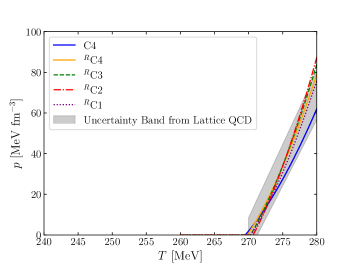
Figure 2: Deconfinement phase transition for the pure gauge case for different vector couplings with lattice QCD error band taken from Ref. [126].

III.2.2 Pseudo critical transition temperature

The chiral phase transition and the deconfinement phase transitions are distinct yet seem to be interconnected phenomena in QCD (at least at $\mu_{B}=0$). The chiral phase transition involves a modification of the QCD vacuum characterized by condensates, crucial for generating hadron masses with chiral symmetry restoration occurring at high temperatures and/or baryonic densities. Conversely, the deconfinement phase transition marks the transition from hadronic degrees of freedom to quarks and gluons. These transitions are characterized by distinct order parameters (usually $\sigma$ for chiral phase transition and $\Phi$ for deconfinement phase transition). According to lattice QCD findings at $\mu_{B}=0$, the chiral phase transition from the hadronic phase to the quark phase is not a sharp discontinuity but rather a crossover [127]. This crossover’s central point is denoted as the pseudo-critical or crossover transition temperature $T^{p}_{c}$, with a known value of 158 $\pm$ 0.6 MeV as per latest lattice results [15].

In Figure 3, we present the change in the order parameters $\sigma$ and $\Phi$ with temperature at $\mu_{B}=\mu_{Q}=\mu_{S}=0$. In the CMF model, to match the constraints from the theory, we perform parameter fitting for $T_{0}$ and $g_{q\Phi}$, whose values are provided in Table 7. The figure illustrates that the chiral condensate ($\sigma$) is equal to its vacuum value ($\sigma_{0}$) in the low-temperature regime. However, as $T$ increases, $\sigma$ decreases, indicating the transition from the chiral broken phase into the chiral restored phase. Additionally, the maximum change in the chiral condensate (peak of chiral susceptibility) occurs around $T^{p}_{c}=$161 MeV for all renormalized coupling schemes, and these values are tabulated in Table 8. Note that, in our model the maximum change in the deconfinement order parameter $\Phi$ is approximately the same as the maximum change in the chiral condensate $\sigma$. For reference, we also mention the value of $T^{p}_{c}$ for the older unrenormalized C4 coupling, which was initially fixed based on the older constraint of the pseudo-critical transition temperature [63], and therefore presents slightly different results.

Table 8: Pseudo-critical temperature for different vector couplings.

Coupling	$T^{p}_{c}$(MeV)
RC1	162.40
RC2	158.90
RC3	161.65
RC4	162.70
C4	170.82

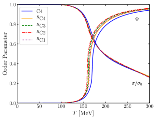
Figure 3: Chiral symmetry restoration represented by the condensate $\sigma$ and deconfinement represented by $\Phi$ for different couplings at $\mu_{B}=\mu_{S}=\mu_{Q}=0$.

III.2.3 Deconfinement critical point

The transition from hadronic to quark phase is characterized by a crossover at low values of baryon chemical potential, but it is believed that eventually a critical point is reached at $\mu_{B}$, beyond which a first-order phase transition line exists [128]. The existence of a critical point is supported by symmetry arguments together with an indication from experiments, where hints of a critical point have been seen in net-proton fluctuation data from the STAR’s Beam Energy Scan [129]. This phase transition line would intersect the $T=0$ axis at a point a few times the nuclear saturation density. On the theory side, recent lattice QCD results have not shown signs of critical behavior up to $\mu_{B}\approx 300$ MeV, with a critical temperature estimated to be less than $T^{HQ}_{c}<132^{+3}_{-6}$ MeV [15, 17]. A machine learning approach in [130] based on the lattice QCD equation of state coupled to a critical point found on the grounds of causality and stability found that the critical point is heavily skewed towards $\mu_{B}\gtrsim 400$ MeV. To accommodate these constraints, we adjust our model (as provided in Table 7) to position the critical point at temperatures lower than $T<135$ MeV and baryon chemical potentials greater than $\mu_{B}>300$. Note that in a study that used the holographic gauge/gravity correspondence to map out the QCD phase diagram [131], the authors of [132] were able to constrain the location of the critical point at $T_{c}\sim 105$ MeV and $\mu_{B,c}\sim 580$ MeV by using a Bayesian analysis constrained to state-of-the-art lattice QCD results.

In our model, to locate the critical point in the region provided by first principles, we make adjustments to the $a_{2}$ parameter, which is associated with the mixed term $\mu_{B}^{2}T^{2}$ in the deconfinement potential equation (Eq. 3). This parameter modification has a direct impact on how the phase diagram behaves in the region where both $\mu_{B}$ and temperature $T$ are non-zero. Figure 4 illustrates the first-order deconfinement phase transition lines alongside the respective critical points for various vector coupling schemes. We have also included the phase transition line associated with the unrenormalized C4 coupling scheme, which was fitted to older constraint data. Detailed values of the critical temperature $T_{c}$, and critical baryon chemical potential $\mu_{B,c}$ for different vector couplings are provided in Table 9. In the cases of ^RC1-^RC3, it is notable that the critical point appears naturally at lower values of $\mu_{B}$ and higher values of $T$ (in comparison with ^RC4) no matter how we fix the parameters.

Note that chiral symmetry restoration in the presence of only hadrons appears as a smooth crossover in the CMF model. When quarks are added, a discontinuity in the order parameter $\sigma$ appears whenever there is a discontinuity in the order parameter $\Phi$. Nevertheless, we refer to this as a deconfinement phase transition, as the discontinuity in its order parameter is much larger and at low temperature it switches from having just hadrons to just quarks. The overall change in $\sigma$ and, e.g., baryon masses (away from the discontinuity) is much more gradual.

Table 9: Deconfinement critical point for different couplings.

Coupling	$T^{\rm HQ}_{c}$(MeV)	$\mu_{B,c}$ (MeV)
RC1	132.0	1028.85
RC2	127.9	1042.38
RC3	132.8	1014.26
RC4	113.8	1076.39
C4	167.0	354.00

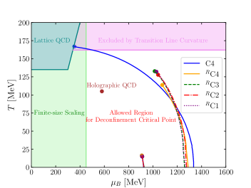
Figure 4: Deconfinement phase transition as well as liquid-gas coexistence lines and respective critical points for $\mu_{Q}=0$ and zero net strangeness. The shaded regions show the exclusion of quark hadron critical point by Lattice QCD [133], finite-size scaling [134], and transition line curvature [135]. It also shows a critical point from holographic QCD [131, 132].

III.2.4 Liquid-gas critical point

In the context of nuclear physics, the term “liquid-gas phase transition” is often used to describe a phase transition akin to what is observed in the behavior of ordinary liquids and gases. In this scenario, the transition occurs within nuclear matter, which transitions from a phase of nuclei (analogous to a gaseous phase) to bulk nuclear matter (analogous to a more dense liquid phase). In our model, we do not have nuclei as explicit degrees of freedom, making it a vacuum-to-bulk nuclear matter phase transition. Similar to the hadron-quark crossover observed at low baryon chemical potentials, the liquid-gas phase transition also becomes a crossover beyond a threshold temperature. The point that separates the crossover regime from the first-order line is then a critical point $T^{\rm LG}_{c}$. Beyond this point, it features a distinct discontinuous line known as the liquid-gas phase transition.

In this study, we have determined for the first time the liquid-gas critical points for various coupling schemes, as documented in Table 10. We do not include hyperons as their influence (if any) would be very small at such ${\mu_{B}}^{\prime}s$ and $T^{\prime}s$. We have depicted the liquid-gas phase transition lines for different couplings with critical points in Figure 4. This determination is based on the behavior of the chiral condensate $\sigma$ near $\mu_{B}\sim 938$ MeV, which corresponds to the mass of nucleons. The liquid-gas critical points were found (without any parameter fitting) to match experimental observations closely, with values $T^{\rm LG}_{c}$ ranging from 15 to 17 MeV [12, 13, 14]. The couplings C1-C3 present slightly different values than C4. This is due to the unique characteristic of C4 involving a linear term in $\phi$ and consequently different parameterizations including a bare mass term for the baryons.

Table 10: Nuclear liquid-gas critical point for different couplings for $\mu_{Q}=0$.

Coupling	$T^{\rm LG}_{c}$(MeV)	$\mu^{\rm LG}_{B,c}$ (MeV)
RC1	14.91	911.55
RC2	14.91	911.55
RC3	14.91	911.55
RC4	16.34	908.94
C4	16.41	908.32

III.2.5 Equation of state at T=0

In this section, we delve into the $T=0$ axis of the QCD phase diagram, which is approximated by matter in the interior of fully evolved (beyond the proto-neutron star stage) neutron stars. At $T=0$, the EoS elucidates the intricate relationship between various thermodynamic properties of matter within a neutron star and can help to reveal the relevant microscopic degrees of freedom. Leptons (electrons and muons) are included through chemical equilibrium, i.e., $\mu_{e}=\mu_{\mu}=-\mu_{Q}$, where $\mu_{Q}$ is determined by ensuring charge neutrality. $\mu_{S}$ is set to zero, since strangeness is allowed to increase.

In Figure 5, we present pressure versus number density at $T=0$ for four different configurations (one shown also with hyperons). As previously discussed, our model incorporates a deconfinement potential (see Eq. 3) designed to transition between hadronic and quark contributions. In the figure, for each coupling scheme, we observe an increase in Fermi pressure within the hadronic system as the number density rises, ultimately culminating in a strong first-order phase transition. This transition results in a substantial increase in number density as the pressure surges in the quark regime. Within our newly proposed parametrization, by adjusting the quark couplings to $\Phi$ i.e. $g_{q\Phi}$, we arrive at a smaller (more realistic) number density jump during the phase transition compared to the old C4 scheme.

In our quest to gain deeper insights into the threshold of the hadron-to-quark phase transition, characterized by the critical baryonic deconfinement density ($n^{d}_{B,c}$), we have adjusted the parameter $a_{1}$ to obtain a lower value of $n^{d}_{B,c}$, typically ranging around 3.4 $n_{\mathrm{sat}}$ (compatible with the approximate range of density at which baryons start to overlap). For reference, we have compiled the values of critical densities ($n^{d}_{B,c}$) obtained within our work in Table 11. Furthermore, the degree of softness or stiffness in the EoS serves as a key determinant of a neutron star’s ability to resist gravitational collapse. From the behavior of pressure versus energy density in the quark sector (not shown here), we observe that all of the new coupling schemes exhibit stiffer pressures compared to the old C4 scheme. We also find that in the ^RC4 coupling scheme the stiffness (pressure in relation to number/energy density) is almost the same, independently of the presence of hyperons, as they tend to appear in small numbers. However, the inclusion of hyperons for (^RC1-^RC3) couplings would lead to an extremely soft EoS due to larger number of hyperons. As such scenario is not compatible with recent observations of neutron stars, we chose not to show these results.

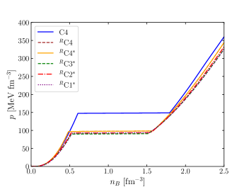
Figure 5: Equation of state for neutron-star matter at $T=0$ for different vector couplings. The symbol $``*"$ marks the cases that do not include hyperons at $T$=0.

Table 11: Starting point of deconfinement phase transition for neutron-star matter at $T=0$ using different vector couplings. The symbol $``*"$ marks cases that do not that include hyperons at $T$=0.

Coupling	$n^{d}_{B,c}(n_{\mathrm{sat}})$
RC1∗	3.53
RC2∗	3.44
RC3∗	3.46
RC4∗	3.22
RC4	3.22
C4	4.00

In Figure 6, we depict the mass-radius curves for various renormalized coupling schemes, both with and without hyperons, within a system governed by hadronic degrees of freedom. To provide context, we also include the mass-radius curve from our widely used work (unrenormalized C4 coupling with hyperons) [64, 63, 66, 99, 100, 101, 68, 136, 67, 69, 70, 71, 72, 73, 119]. When examining hadronic matter without hyperons, we observe that the renormalized ^RC4 coupling scheme yields the highest maximum mass ($M_{\rm max}$), which can be compared to other renormalized coupling schemes and the unrenormalized C4 scheme. The inclusion of hyperons results in a slight reduction in $M_{\rm max}$ for ^RC4, but it still remains higher than the other coupling schemes. From the figure, for ^RC4 we can conclude that the incorporation of renormalized vector fields leads to a stiffer EoS, resulting in a higher $M_{\rm max}$. On the other hand, for the other renormalized coupling schemes (^RC1-^RC3), we also achieve a $M_{max}$ of approximately $2M_{\odot}$.

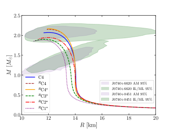
Figure 6: Mass-radius curve for neutron star matter with different renormalized vector coupling including a BPS crust [125]. The shaded regions in color green denote the NICER data for PSR J0030+6620 and J0740+0451, employing the Illinois-Maryland analysis [38]. Meanwhile, the violet region illustrates the NICER data for the same pulsars analyzed through the Amsterdam analysis [39]. The symbol $``*"$ marks the cases that do not include hyperons at $T$=0.

Concerning radius and by extension tidal deformability, better agreement with the results from NICER [38, 39], LIGO and VIRGO [40] can be achieved by modifying the vector-isovector interactions ($\omega\rho$). This has been explored, e.g., in Refs. [137, 138, 139, 140, 141, 142, 143, 144, 145, 146, 147] and in the CMF model [100, 64, 99, 122]. In the present work, we do not focus on vector-isovector interactions because they do not modify the finite temperature part of the QCD phase diagram. Also, we did not vary the crust in the present work but a different crust will influence agreement with LIGO/NICER constraints. While we now have a complete equation of state that includes the deconfinement phase transition, a thorough study of its macroscopic properties on neutron stars will wait for a later work. The primary reason is that including the EoS as it is in the TOV equations implies that the surface tension of quark matter is infinite, which would generate an impenetrable “wall” between the hadronic and quark phases. Under the influence of gravity, points with similar pressure would be side by side and there would be no region with the baryon densities corresponding to the jump in Figure 5. In this case, the mass-radius diagram would show a kink. To assess the stability of the star in the decreasing mass branch, we would have to consider the speed of hadron$\leftrightarrow$quark conversion [148], which could in turn make hybrid stars unstable. Second, if the surface tension of quark matter is below a certain threshold, a mixture of phases appears, which enhances stellar stability. In this case, another dimension ($\mu_{Q}$) appears, which allows the baryon density to increase smoothly while connecting the hadronic and quark phases [148, 149, 150, 151]. Mixed phases have been extensively studied within the CMF model [71, 72] and more will be reported soon.

Alternatively, by altering the deconfined potential (for example, from $a_{1}\mu_{B}^{4}$ to $a_{1}^{\prime}\mu_{B}^{2}$) to make it less responsive to the baryon chemical potential, we can achieve a less pronounced first-order phase transitions, resulting in smaller changes in baryon density across the deconfinement phase transition even for infinite surface tension [152, 153, 154, 155, 156, 157]. This facilitates producing stable hybrid stars without mixed phases [136, 101, 122].

IV Conclusion

In this work we take the CMF model, which can describe most key features across the QCD phase diagram, and break degeneracies in the mass of the vector mesons for the first time. We explore different self-interaction vector couplings (C1-C4) and for the first time, we study some of them (C1-C3) including deconfinement to quark matter and finite temperature effects. These crucial steps give us a better understanding of the role of vector mesons play in the equation of state and pave the way for future studies of in-medium masses of thermal meson within the CMF model. Because of the complexity of the CMF model and its inherent interconnectedness across the entire phase diagram, the changes we make also required a full revision of the model. Furthermore, over the past decade significant advances have been made across the QCD phase diagram. We incorporate these new constraints in the latest parameterization of the CMF model for the first time in this work as well.

As the vector mesons play a crucial role in mediating the repulsive forces between baryons and quarks, their renormalization strongly affects the properties of hadronic and quark matter. Therefore, the entire model needs to be re-parameterized. By incorporating appropriate chiral invariants into the vector interactive Lagrangian, we successfully eliminate the mass degeneracy among the vector mesons by refitting the parameters related to the mass term of the vector meson Lagrangian, aligning them more closely with empirical data. We also discuss the fitting of parameters for the baryon/quark-meson interaction and self-interacting vector mesons. These adjustments aim to match key modern experimental constraints, such as the saturation density, the binding energy per nucleon, the compressibility, the symmetry energy, the slope parameter, and the Lambda hyperon potential in addition to constraints for the liquid-gas critical point and constraints from astrophysics. In particular, we find that the redefinition of vector fields plays a significant role in reproducing neutron stars with higher masses, when compared to the previous unrenormalized field definitions.

Furthermore, we explore the parameters associated with the Polyakov-inspired deconfinement potential. This includes reproducing lattice QCD constraints, such as the location of the deconfinement phase transition, the pseudo-critical transition temperature, and constraints that exclude the location of the hadron-quark critical point in certain regions of the phase diagram. The uniqueness of our new parameter fit is grounded in our careful selection of distinctive constants by spanning the search over a whole phase diagram, encompassing novel constraints not previously considered in the field. Rigorous validation, including extensive consistency checks, demonstrates the robustness of our results.

Looking forward, this work opens up multiple new avenues to explore. For starters, we can study the effect of the new renormalization schemes on the in-medium masses of thermal mesons, which haven’t yet been considered. At the moment, we can easily add a gas of free thermal mesons to our calculations, but they would be present in both hadronic and quark phases. Once in-medium masses guarantee that the thermal mesons are suppressed in the quark phase, then, we can use a wider set of lattice QCD results to fit or test our formalism, such as partial pressures [158]. On the experimental side, the EoS derived from the CMF model can be used to connect the physics of neutron stars with that of heavy-ion collisions when exploring different isospin and strangeness. The EoS at $T=0$ is valuable for gaining insights into both the micro- and macroscopic properties of neutron stars, providing a framework to study, e.g., different net strangeness and quark content in neutron stars, as well as input for simulations of neutron-star cooling and, in the case of finite $T$, input for simulations of neutron star mergers and supernovae. It would be interesting to study these new parametrizations of the CMF EoS in different astrophysical scenarios and also in simulations of heavy-ion collisions. Finally, the knowledge gained on the effect of the parameters across the entire CMF model in terms of how they connect to key features of the QCD phase diagram will play an important role in future work (such as a Bayesian analysis) that uses statistical methods to constrain model parameters.

Appendix A Particle Multiplets

• Baryon Matrix

  $$B=\begin{pmatrix}\frac{\Sigma^{0}}{\sqrt{2}}+\frac{\Lambda_{0}}{\sqrt{6}}&\Sigma^{+}&p\\ \Sigma^{-}&\frac{-\Sigma^{0}}{\sqrt{2}}+\frac{\Lambda^{0}}{\sqrt{6}}&n\\ \Xi^{-}&\Xi^{0}&-2\frac{\Lambda^{0}}{\sqrt{6}}\end{pmatrix}$$ (28)

• Scalar Matrix

  $$X=\begin{pmatrix}\frac{\delta^{0}+\sigma}{\sqrt{2}}&\delta^{+}&\kappa^{+}\\ \delta^{-}&\frac{-\delta^{0}+\sigma}{\sqrt{2}}&\kappa^{0}\\ \kappa^{-}&\bar{\kappa}^{0}&\zeta\end{pmatrix}$$ (29)

• Scalar Matrix in the Mean-field Approximation

  $$\left\langle X\right\rangle=\begin{pmatrix}\frac{\delta^{0}+\sigma}{\sqrt{2}}&0&0\\ 0&\frac{-\delta^{0}+\sigma}{\sqrt{2}}&0\\ 0&0&\zeta\end{pmatrix}$$ (30)

• Vector Meson Matrix

  $$V_{\mu}=\begin{pmatrix}\frac{\rho^{0}_{\mu}+\omega_{\mu}}{\sqrt{2}}&\rho^{+}_{\mu}&K^{*+}_{\mu}\\ \rho^{-}_{\mu}&\frac{-\rho^{0}_{\mu}+\omega_{\mu}}{\sqrt{2}}&K^{*0}_{\mu}\\ K^{*-}_{\mu}&\bar{K}^{*0}_{\mu}&\phi_{\mu}\end{pmatrix}$$ (31)

• Degenerate Vector Meson Matrix

  $$V_{\mu}=\begin{pmatrix}\frac{\rho_{\mu}+\omega_{\mu}}{\sqrt{2}}&\rho_{\mu}&K^{*}_{\mu}\\ \rho_{\mu}&\frac{-\rho_{\mu}+\omega_{\mu}}{\sqrt{2}}&K^{*}_{\mu}\\ K^{*}_{\mu}&\bar{K}^{*}_{\mu}&\phi_{\mu}\end{pmatrix}$$ (32)

• Degenerate Vector Meson Tensor Matrix

  $$V^{\mu\nu}=\begin{pmatrix}\frac{V^{\mu\nu}_{\rho}+V^{\mu\nu}_{\omega}}{\sqrt{2}}&V^{\mu\nu}_{\rho}&V^{\mu\nu}_{K^{*}}\\ V^{\mu\nu}_{\rho}&\frac{-V^{\mu\nu}_{\rho}+V^{\mu\nu}_{\omega}}{\sqrt{2}}&V^{\mu\nu}_{K^{*}}\\ V^{\mu\nu}_{K^{*}}&V^{\mu\nu}_{\bar{K}^{*}}&V^{\mu\nu}_{\phi}\end{pmatrix}$$ (33)

References

- Dexheimer et al. [2021a] V. Dexheimer, J. Noronha, J. Noronha-Hostler, C. Ratti, and N. Yunes, Future physics perspectives on the equation of state from heavy ion collisions to neutron stars, J. Phys. G 48, 073001 (2021a), arXiv:2010.08834 [nucl-th] .
- Lovato et al. [2022] A. Lovato et al., Long Range Plan: Dense matter theory for heavy-ion collisions and neutron stars (2022), arXiv:2211.02224 [nucl-th] .
- Sorensen et al. [2023] A. Sorensen et al., Dense Nuclear Matter Equation of State from Heavy-Ion Collisions (2023), arXiv:2301.13253 [nucl-th] .
- Heinz [2001] U. W. Heinz, The Little bang: Searching for quark gluon matter in relativistic heavy ion collisions, Nucl. Phys. A 685, 414 (2001), arXiv:hep-ph/0009170 .
- Vogt [2007] R. Vogt, Ultrarelativistic heavy-ion collisions (Elsevier, Amsterdam, 2007).
- Baym et al. [2018] G. Baym, T. Hatsuda, T. Kojo, P. D. Powell, Y. Song, and T. Takatsuka, From hadrons to quarks in neutron stars: a review, Rept. Prog. Phys. 81, 056902 (2018), arXiv:1707.04966 [astro-ph.HE] .
- Lattimer [2021] J. M. Lattimer, Neutron Stars and the Nuclear Matter Equation of State, Ann. Rev. Nucl. Part. Sci. 71, 433 (2021).
- Burgio et al. [2021] G. F. Burgio, H. J. Schulze, I. Vidana, and J. B. Wei, Neutron stars and the nuclear equation of state, Prog. Part. Nucl. Phys. 120, 103879 (2021), arXiv:2105.03747 [nucl-th] .
- Annala et al. [2020] E. Annala, T. Gorda, A. Kurkela, J. Nättilä, and A. Vuorinen, Evidence for quark-matter cores in massive neutron stars, Nature Phys. 16, 907 (2020), arXiv:1903.09121 [astro-ph.HE] .
- Philipsen [2013] O. Philipsen, The QCD equation of state from the lattice, Prog. Part. Nucl. Phys. 70, 55 (2013), arXiv:1207.5999 [hep-lat] .
- Ratti [2018] C. Ratti, Lattice QCD and heavy ion collisions: a review of recent progress, Rept. Prog. Phys. 81, 084301 (2018), arXiv:1804.07810 [hep-lat] .
- Natowitz et al. [2002] J. B. Natowitz, K. Hagel, Y. Ma, M. Murray, L. Qin, R. Wada, and J. Wang, Limiting temperatures and the equation of state of nuclear matter, Phys. Rev. Lett. 89, 212701 (2002), arXiv:nucl-ex/0204015 .
- Karnaukhov et al. [2008] V. A. Karnaukhov et al., Critical temperature for the nuclear liquid-gas phase transition (from multifragmentation and fission), Phys. Atom. Nucl. 71, 2067 (2008), arXiv:0801.4485 [nucl-ex] .
- Elliott et al. [2013] J. B. Elliott, P. T. Lake, L. G. Moretto, and L. Phair, Determination of the coexistence curve, critical temperature, density, and pressure of bulk nuclear matter from fragment emission data, Phys. Rev. C 87, 054622 (2013).
- Borsanyi et al. [2020] S. Borsanyi, Z. Fodor, J. N. Guenther, R. Kara, S. D. Katz, P. Parotto, A. Pasztor, C. Ratti, and K. K. Szabo, QCD Crossover at Finite Chemical Potential from Lattice Simulations, Phys. Rev. Lett. 125, 052001 (2020), arXiv:2002.02821 [hep-lat] .
- Borsányi et al. [2021] S. Borsányi, Z. Fodor, J. N. Guenther, R. Kara, S. D. Katz, P. Parotto, A. Pásztor, C. Ratti, and K. K. Szabó, Lattice QCD equation of state at finite chemical potential from an alternative expansion scheme, Phys. Rev. Lett. 126, 232001 (2021), arXiv:2102.06660 [hep-lat] .
- Ding et al. [2019] H. T. Ding et al. (HotQCD), Chiral Phase Transition Temperature in ( 2+1 )-Flavor QCD, Phys. Rev. Lett. 123, 062002 (2019), arXiv:1903.04801 [hep-lat] .
- Roessner et al. [2007] S. Roessner, C. Ratti, and W. Weise, Polyakov loop, diquarks and the two-flavour phase diagram, Phys. Rev. D 75, 034007 (2007), arXiv:hep-ph/0609281 .
- Adhikari et al. [2021] D. Adhikari et al. (PREX), Accurate Determination of the Neutron Skin Thickness of 208Pb through Parity-Violation in Electron Scattering, Phys. Rev. Lett. 126, 172502 (2021), arXiv:2102.10767 [nucl-ex] .
- Myers and Swiatecki [1966] W. D. Myers and W. J. Swiatecki, Nuclear masses and deformations, Nucl. Phys. 81, 1 (1966).
- Myers and Swiatecki [1996] W. D. Myers and W. J. Swiatecki, Nuclear properties according to the Thomas-Fermi model, Nucl. Phys. A 601, 141 (1996).
- Colo et al. [2014] G. Colo, U. Garg, and H. Sagawa, Symmetry energy from the nuclear collective motion: constraints from dipole, quadrupole, monopole and spin-dipole resonances, Eur. Phys. J. A 50, 26 (2014), arXiv:1309.1572 [nucl-th] .
- Todd-Rutel and Piekarewicz [2005] B. G. Todd-Rutel and J. Piekarewicz, Neutron-Rich Nuclei and Neutron Stars: A New Accurately Calibrated Interaction for the Study of Neutron-Rich Matter, Phys. Rev. Lett. 95, 122501 (2005), arXiv:nucl-th/0504034 .
- Colo et al. [2004] G. Colo, N. Van Giai, J. Meyer, K. Bennaceur, and P. Bonche, Microscopic determination of the nuclear incompressibility within the nonrelativistic framework, Phys. Rev. C 70, 024307 (2004), arXiv:nucl-th/0403086 .
- Agrawal et al. [2003] B. K. Agrawal, S. Shlomo, and V. K. Au, Nuclear matter incompressibility coefficient in relativistic and nonrelativistic microscopic models, Phys. Rev. C 68, 031304 (2003), arXiv:nucl-th/0308042 .
- Stone et al. [2014] J. R. Stone, N. J. Stone, and S. A. Moszkowski, Incompressibility in finite nuclei and nuclear matter, Phys. Rev. C 89, 044316 (2014), arXiv:1404.0744 [nucl-th] .
- Yao et al. [2023] N. Yao, A. Sorensen, V. Dexheimer, and J. Noronha-Hostler, Structure in the speed of sound: from neutron stars to heavy-ion collisions (2023), arXiv:2311.18819 [nucl-th] .
- Li et al. [2019] B.-A. Li, P. G. Krastev, D.-H. Wen, and N.-B. Zhang, Towards Understanding Astrophysical Effects of Nuclear Symmetry Energy, Eur. Phys. J. A 55, 117 (2019), arXiv:1905.13175 [nucl-th] .
- Fan et al. [2014] X. Fan, J. Dong, and W. Zuo, Density-dependent symmetry energy at subsaturation densities from nuclear mass differences, Phys. Rev. C 89, 017305 (2014), arXiv:1403.2055 [nucl-th] .
- Reed et al. [2021] B. T. Reed, F. J. Fattoyev, C. J. Horowitz, and J. Piekarewicz, Implications of PREX-2 on the Equation of State of Neutron-Rich Matter, Phys. Rev. Lett. 126, 172503 (2021), arXiv:2101.03193 [nucl-th] .
- Reinhard et al. [2021] P.-G. Reinhard, X. Roca-Maza, and W. Nazarewicz, Information Content of the Parity-Violating Asymmetry in Pb208, Phys. Rev. Lett. 127, 232501 (2021), arXiv:2105.15050 [nucl-th] .
- Millener et al. [1988] D. J. Millener, C. B. Dover, and A. Gal, Lambda Nucleus Single Particle Potentials, Phys. Rev. C 38, 2700 (1988).
- Fortin et al. [2018] M. Fortin, M. Oertel, and C. Providência, Hyperons in hot dense matter: what do the constraints tell us for equation of state?, Publ. Astron. Soc. Austral. 35, 44 (2018), arXiv:1711.09427 [astro-ph.HE] .
- Gal et al. [2016] A. Gal, E. V. Hungerford, and D. J. Millener, Strangeness in nuclear physics, Rev. Mod. Phys. 88, 035004 (2016), arXiv:1605.00557 [nucl-th] .
- Fabbietti et al. [2021] L. Fabbietti, V. Mantovani Sarti, and O. Vazquez Doce, Study of the Strong Interaction Among Hadrons with Correlations at the LHC, Ann. Rev. Nucl. Part. Sci. 71, 377 (2021), arXiv:2012.09806 [nucl-ex] .
- Collaboration et al. [2020] A. Collaboration et al. (ALICE), Unveiling the strong interaction among hadrons at the LHC, Nature 588, 232 (2020), [Erratum: Nature 590, E13 (2021)], arXiv:2005.11495 [nucl-ex] .
- Inoue [2019] T. Inoue (HAL QCD), Hyperon Forces from QCD and Their Applications, JPS Conf. Proc. 26, 023018 (2019).
- Miller et al. [2019] M. C. Miller et al., PSR J0030+0451 Mass and Radius from Data and Implications for the Properties of Neutron Star Matter, Astrophys. J. Lett. 887, L24 (2019), arXiv:1912.05705 [astro-ph.HE] .
- Riley et al. [2019] T. E. Riley et al., A View of PSR J0030+0451: Millisecond Pulsar Parameter Estimation, Astrophys. J. Lett. 887, L21 (2019), arXiv:1912.05702 [astro-ph.HE] .
- Abbott et al. [2018] B. P. Abbott et al. (LIGO Scientific, Virgo), GW170817: Measurements of neutron star radii and equation of state, Phys. Rev. Lett. 121, 161101 (2018), arXiv:1805.11581 [gr-qc] .
- Kumar et al. [2018] R. Kumar et al., Theoretical and Experimental Constraints for the Equation of State of Dense and Hot Matter (2018), arXiv:2303.17021 [nucl-th] .
- Troyer and Wiese [2005] M. Troyer and U.-J. Wiese, Computational complexity and fundamental limitations to fermionic quantum Monte Carlo simulations, Phys. Rev. Lett. 94, 170201 (2005), arXiv:cond-mat/0408370 .
- Muroya et al. [2003] S. Muroya, A. Nakamura, C. Nonaka, and T. Takaishi, Lattice QCD at finite density: An Introductory review, Prog. Theor. Phys. 110, 615 (2003), arXiv:hep-lat/0306031 .
- de Forcrand [2009] P. de Forcrand, Simulating QCD at finite density, PoS LAT2009, 010 (2009), arXiv:1005.0539 [hep-lat] .
- Andersen and Strickland [2002] J. O. Andersen and M. Strickland, The Equation of state for dense QCD and quark stars, Phys. Rev. D 66, 105001 (2002), arXiv:hep-ph/0206196 .
- Fraga et al. [2014] E. S. Fraga, A. Kurkela, and A. Vuorinen, Interacting quark matter equation of state for compact stars, Astrophys. J. Lett. 781, L25 (2014), arXiv:1311.5154 [nucl-th] .
- Kurkela and Vuorinen [2016] A. Kurkela and A. Vuorinen, Cool quark matter, Phys. Rev. Lett. 117, 042501 (2016), arXiv:1603.00750 [hep-ph] .
- Andersen et al. [1999] J. O. Andersen, E. Braaten, and M. Strickland, Hard thermal loop resummation of the free energy of a hot gluon plasma, Phys. Rev. Lett. 83, 2139 (1999), arXiv:hep-ph/9902327 .
- Andersen et al. [2000a] J. O. Andersen, E. Braaten, and M. Strickland, Hard thermal loop resummation of the thermodynamics of a hot gluon plasma, Phys. Rev. D 61, 014017 (2000a), arXiv:hep-ph/9905337 .
- Andersen et al. [2000b] J. O. Andersen, E. Braaten, and M. Strickland, Hard thermal loop resummation of the free energy of a hot quark - gluon plasma, Phys. Rev. D 61, 074016 (2000b), arXiv:hep-ph/9908323 .
- Tews et al. [2013] I. Tews, T. Krüger, K. Hebeler, and A. Schwenk, Neutron matter at next-to-next-to-next-to-leading order in chiral effective field theory, Phys. Rev. Lett. 110, 032504 (2013), arXiv:1206.0025 [nucl-th] .
- Walecka [1974] J. Walecka, A theory of highly condensed matter, Annals of Physics 83, 491 (1974).
- Nambu and Jona-Lasinio [1961] Y. Nambu and G. Jona-Lasinio, Dynamical Model of Elementary Particles Based on an Analogy with Superconductivity. 1., Phys. Rev. 122, 345 (1961).
- Fukushima [2004] K. Fukushima, Chiral effective model with the Polyakov loop, Phys. Lett. B 591, 277 (2004), arXiv:hep-ph/0310121 .
- Schaffner-Bielich and Randrup [1999] J. Schaffner-Bielich and J. Randrup, DCC dynamics with the SU(3) linear sigma model, Phys. Rev. C 59, 3329 (1999), arXiv:nucl-th/9812032 .
- Weinberg [1968] S. Weinberg, Nonlinear realizations of chiral symmetry, Phys. Rev. 166, 1568 (1968).
- Gallas et al. [2010] S. Gallas, F. Giacosa, and D. H. Rischke, Vacuum phenomenology of the chiral partner of the nucleon in a linear sigma model with vector mesons, Phys. Rev. D 82, 014004 (2010), arXiv:0907.5084 [hep-ph] .
- Kovács et al. [2022] P. Kovács, J. Takátsy, J. Schaffner-Bielich, and G. Wolf, Neutron star properties with careful parametrization in the vector and axial-vector meson extended linear sigma model, Phys. Rev. D 105, 103014 (2022), arXiv:2111.06127 [nucl-th] .
- Papazoglou et al. [1999] P. Papazoglou, D. Zschiesche, S. Schramm, J. Schaffner-Bielich, H. Stoecker, and W. Greiner, Nuclei in a chiral SU(3) model, Phys. Rev. C 59, 411 (1999), arXiv:nucl-th/9806087 .
- Bonanno and Drago [2009] L. Bonanno and A. Drago, A Chiral lagrangian with Broken Scale: Testing the restoration of symmetries in astrophysics and in the laboratory, Phys. Rev. C 79, 045801 (2009), arXiv:0805.4188 [nucl-th] .
- Kumar and Kumar [2019] R. Kumar and A. Kumar, and in asymmetric hot magnetized nuclear matter: a unified approach of Chiral SU(3) model and QCD sum rules, Eur. Phys. J. C 79, 403 (2019), arXiv:1810.09185 [hep-ph] .
- Motornenko et al. [2020] A. Motornenko, J. Steinheimer, V. Vovchenko, S. Schramm, and H. Stoecker, Equation of state for hot QCD and compact stars from a mean field approach, Phys. Rev. C 101, 034904 (2020), arXiv:1905.00866 [hep-ph] .
- Dexheimer and Schramm [2010] V. A. Dexheimer and S. Schramm, A Novel Approach to Model Hybrid Stars, Phys. Rev. C 81, 045201 (2010), arXiv:0901.1748 [astro-ph.SR] .
- Dexheimer and Schramm [2008] V. Dexheimer and S. Schramm, Proto-Neutron and Neutron Stars in a Chiral SU(3) Model, Astrophys. J. 683, 943 (2008), arXiv:0802.1999 [astro-ph] .
- Ratti et al. [2006a] C. Ratti, M. A. Thaler, and W. Weise, Phases of QCD: Lattice thermodynamics and a field theoretical model, Rom. Rep. Phys. 58, 13 (2006a).
- Dexheimer et al. [2012] V. Dexheimer, R. Negreiros, and S. Schramm, Hybrid Stars in a Strong Magnetic Field, Eur. Phys. J. A 48, 189 (2012), arXiv:1108.4479 [astro-ph.HE] .
- Franzon et al. [2016] B. Franzon, V. Dexheimer, and S. Schramm, A self-consistent study of magnetic field effects on hybrid stars, Mon. Not. Roy. Astron. Soc. 456, 2937 (2016), arXiv:1508.04431 [astro-ph.HE] .
- Dexheimer et al. [2021b] V. Dexheimer, K. D. Marquez, and D. P. Menezes, Delta baryons in neutron-star matter under strong magnetic fields, Eur. Phys. J. A 57, 216 (2021b), arXiv:2103.09855 [nucl-th] .
- Marquez et al. [2022] K. D. Marquez, M. R. Pelicer, S. Ghosh, J. Peterson, D. Chatterjee, V. Dexheimer, and D. P. Menezes, Exploring the effects of baryons in magnetars, Phys. Rev. C 106, 035801 (2022), arXiv:2205.09827 [astro-ph.HE] .
- Peterson et al. [2023] J. Peterson, P. Costa, R. Kumar, V. Dexheimer, R. Negreiros, and C. Providencia, Temperature and strong magnetic field effects in dense matter, Phys. Rev. D 108, 063011 (2023), arXiv:2304.02454 [nucl-th] .
- Hempel et al. [2013] M. Hempel, V. Dexheimer, S. Schramm, and I. Iosilevskiy, Noncongruence of the nuclear liquid-gas and deconfinement phase transitions, Phys. Rev. C 88, 014906 (2013), arXiv:1302.2835 [nucl-th] .
- Roark and Dexheimer [2018] J. Roark and V. Dexheimer, Deconfinement phase transition in proto-neutron-star matter, Phys. Rev. C 98, 055805 (2018), arXiv:1803.02411 [nucl-th] .
- Aryal et al. [2020] K. Aryal, C. Constantinou, R. L. S. Farias, and V. Dexheimer, High-Energy Phase Diagrams with Charge and Isospin Axes under Heavy-Ion Collision and Stellar Conditions, Phys. Rev. D 102, 076016 (2020), arXiv:2004.03039 [nucl-th] .
- Lenzi et al. [2023] C. H. Lenzi, G. Lugones, and C. Vasquez, Hybrid stars with reactive interfaces: Analysis within the Nambu–Jona-Lasinio model, Phys. Rev. D 107, 083025 (2023), arXiv:2304.01898 [nucl-th] .
- Ferreira et al. [2020] M. Ferreira, R. Câmara Pereira, and C. Providência, Quark matter in light neutron stars, Phys. Rev. D 102, 083030 (2020), arXiv:2008.12563 [nucl-th] .
- Lourenço et al. [2021] O. Lourenço, C. H. Lenzi, M. Dutra, E. J. Ferrer, V. de la Incera, L. Paulucci, and J. E. Horvath, Tidal deformability of strange stars and the GW170817 event, Phys. Rev. D 103, 103010 (2021), arXiv:2104.07825 [astro-ph.HE] .
- Pisarski [2021] R. D. Pisarski, Remarks on nuclear matter: How an condensate can spike the speed of sound, and a model of baryons, Phys. Rev. D 103, L071504 (2021), arXiv:2101.05813 [nucl-th] .
- Lopes [2022] L. L. Lopes, Hyperonic neutron stars: reconciliation between nuclear properties and NICER and LIGO/VIRGO results, Commun. Theor. Phys. 74, 015302 (2022), arXiv:2107.02245 [hep-ph] .
- Ma et al. [2022] F. Ma, W. Guo, and C. Wu, Kaon meson condensate in neutron star matter including hyperons, Phys. Rev. C 105, 015807 (2022), arXiv:2202.03001 [nucl-th] .
- Li et al. [2022] F. Li, B.-J. Cai, Y. Zhou, W.-Z. Jiang, and L.-W. Chen, Effects of Isoscalar- and Isovector-scalar Meson Mixing on Neutron Star Structure, Astrophys. J. 929, 183 (2022), arXiv:2202.08705 [nucl-th] .
- Sun et al. [2023] X. Sun, Z. Miao, B. Sun, and A. Li, Astrophysical Implications on Hyperon Couplings and Hyperon Star Properties with Relativistic Equations of States, Astrophys. J. 942, 55 (2023), arXiv:2205.10631 [astro-ph.HE] .
- Pradhan et al. [2023] B. K. Pradhan, D. Chatterjee, R. Gandhi, and J. Schaffner-Bielich, Role of vector self-interaction in neutron star properties, Nucl. Phys. A 1030, 122578 (2023), arXiv:2209.12657 [nucl-th] .
- Thakur et al. [2022] V. Thakur, R. Kumar, P. Kumar, V. Kumar, M. Kumar, C. Mondal, B. K. Agrawal, and S. K. Dhiman, Effects of an isovector scalar meson on the equation of state of dense matter within a relativistic mean field model, Phys. Rev. C 106, 045806 (2022), arXiv:2210.02793 [nucl-th] .
- Kubis et al. [2023] S. Kubis, W. Wójcik, D. A. Castillo, and N. Zabari, Relativistic mean field model for ultra-compact low mass neutron star of HESS J1731-347 (2023), arXiv:2307.02979 [nucl-th] .
- Câmara Pereira et al. [2016] R. Câmara Pereira, P. Costa, and C. Providência, Two-solar-mass hybrid stars: a two model description with the Nambu-Jona-Lasinio quark model, Phys. Rev. D 94, 094001 (2016), arXiv:1610.06435 [nucl-th] .
- Wu et al. [2018] X. Wu, A. Ohnishi, and H. Shen, Effects of quark-matter symmetry energy on hadron-quark coexistence in neutron-star matter, Phys. Rev. C 98, 065801 (2018), arXiv:1806.03760 [nucl-th] .
- Malfatti et al. [2019] G. Malfatti, M. G. Orsaria, G. A. Contrera, F. Weber, and I. F. Ranea-Sandoval, Hot quark matter and (proto-) neutron stars, Phys. Rev. C 100, 015803 (2019), arXiv:1907.06597 [nucl-th] .
- Lopes and Menezes [2021] L. L. Lopes and D. P. Menezes, Broken SU(6) symmetry and massive hybrid stars, Nucl. Phys. A 1009, 122171 (2021), arXiv:2004.07909 [astro-ph.HE] .
- Alaverdyan [2021] G. Alaverdyan, Hadron–Quark Phase Transition in the SU (3) Local Nambu–Jona-Lasinio (NJL) Model with Vector Interaction, Symmetry 13, 124 (2021), arXiv:2011.12593 [nucl-th] .
- Cao et al. [2022] Z. Cao, L.-W. Chen, P.-C. Chu, and Y. Zhou, GW190814: Circumstantial evidence for up-down quark star, Phys. Rev. D 106, 083007 (2022), arXiv:2009.00942 [astro-ph.HE] .
- Otto et al. [2020] K. Otto, M. Oertel, and B.-J. Schaefer, Nonperturbative quark matter equations of state with vector interactions, Eur. Phys. J. ST 229, 3629 (2020), arXiv:2007.07394 [hep-ph] .
- Marczenko et al. [2020] M. Marczenko, D. Blaschke, K. Redlich, and C. Sasaki, Toward a unified equation of state for multi-messenger astronomy, Astron. Astrophys. 643, A82 (2020), arXiv:2004.09566 [astro-ph.HE] .
- Benic et al. [2015] S. Benic, D. Blaschke, D. E. Alvarez-Castillo, T. Fischer, and S. Typel, A new quark-hadron hybrid equation of state for astrophysics - I. High-mass twin compact stars, Astron. Astrophys. 577, A40 (2015), arXiv:1411.2856 [astro-ph.HE] .
- Miyatsu et al. [2022] T. Miyatsu, M.-K. Cheoun, and K. Saito, Asymmetric Nuclear Matter in Relativistic Mean-field Models with Isoscalar- and Isovector-meson Mixing, Astrophys. J. 929, 82 (2022), arXiv:2202.06468 [nucl-th] .
- Singh et al. [2014] S. K. Singh, S. K. Biswal, M. Bhuyan, and S. K. Patra, Effects of mesons in relativistic mean field theory, Phys. Rev. C 89, 044001 (2014).
- Lopes and Menezes [2020] L. L. Lopes and D. P. Menezes, Role of vector channel in different classes of (non) magnetized neutron stars, Eur. Phys. J. A 56, 122 (2020), arXiv:1909.05400 [astro-ph.HE] .
- Kumari and Kumar [2021] M. Kumari and A. Kumar, Quark Matter within Polyakov Chiral SU(3) Quark Mean Field Model at Finite Temperature, Eur. Phys. J. Plus 136, 19 (2021), arXiv:2003.12780 [hep-ph] .
- Kumar and Kumar [2020] R. Kumar and A. Kumar, meson mass and decay width in strange hadronic matter, Phys. Rev. C 102, 045206 (2020), arXiv:2005.05133 [hep-ph] .
- Dexheimer et al. [2015] V. Dexheimer, R. Negreiros, and S. Schramm, Reconciling Nuclear and Astrophysical Constraints, Phys. Rev. C 92, 012801 (2015), arXiv:1503.07785 [astro-ph.HE] .
- Dexheimer et al. [2019] V. Dexheimer, R. de Oliveira Gomes, S. Schramm, and H. Pais, What do we learn about vector interactions from GW170817?, J. Phys. G 46, 034002 (2019), arXiv:1810.06109 [nucl-th] .
- Dexheimer et al. [2021c] V. Dexheimer, R. O. Gomes, T. Klähn, S. Han, and M. Salinas, GW190814 as a massive rapidly rotating neutron star with exotic degrees of freedom, Phys. Rev. C 103, 025808 (2021c), arXiv:2007.08493 [astro-ph.HE] .
- Ye et al. [2023] J. Ye, J. Margueron, N. Li, and W. Z. Jiang, Zero-sound modes for the nuclear equation of state at supra-normal densities, Phys. Rev. C 108, 044312 (2023), arXiv:2310.16759 [nucl-th] .
- Cierniak et al. [2018] M. Cierniak, T. Klähn, T. Fischer, and N.-U. Bastian, Vector-Interaction-Enhanced Bag Model, Universe 4, 30 (2018), arXiv:1802.03214 [nucl-th] .
- Kojo [2019] T. Kojo, Delineating the properties of matter in cold, dense QCD, AIP Conf. Proc. 2127, 020023 (2019), arXiv:1904.05080 [astro-ph.HE] .
- Shahrbaf et al. [2020] M. Shahrbaf, D. Blaschke, A. G. Grunfeld, and H. R. Moshfegh, First-order phase transition from hypernuclear matter to deconfined quark matter obeying new constraints from compact star observations, Phys. Rev. C 101, 025807 (2020), arXiv:1908.04740 [nucl-th] .
- Wu et al. [2020] Z.-Q. Wu, Chao-Shi, J.-L. Ping, and H.-S. Zong, Contributions of the vector-channel at finite isospin chemical potential with the self-consistent mean field approximation, Phys. Rev. D 101, 074008 (2020), arXiv:2003.02988 [hep-ph] .
- Sun et al. [2021] K.-J. Sun, C.-M. Ko, S. Cao, and F. Li, QCD critical point from the Nambu–Jona-Lasino model with a scalar-vector interaction, Phys. Rev. D 103, 014006 (2021), arXiv:2004.05754 [nucl-th] .
- Huang et al. [2022] K. Huang, J. Hu, Y. Zhang, and H. Shen, The Hadron-quark Crossover in Neutron Star within Gaussian Process Regression Method, Astrophys. J. 935, 88 (2022), arXiv:2206.12760 [nucl-th] .
- Kumar et al. [2023a] A. Kumar, V. B. Thapa, and M. Sinha, Hybrid stars are compatible with recent astrophysical observations, Phys. Rev. D 107, 063024 (2023a), arXiv:2303.06387 [astro-ph.HE] .
- Aguirre [2022] R. M. Aguirre, Hyperons, deconfinement, and the speed of sound in neutron stars, Phys. Rev. D 105, 116023 (2022), arXiv:2204.05221 [nucl-th] .
- Zschiesche et al. [2004] D. Zschiesche, A. Mishra, S. Schramm, H. Stoecker, and W. Greiner, In-medium vector meson masses in a chiral SU(3) model, Phys. Rev. C 70, 045202 (2004), arXiv:nucl-th/0302073 .
- Coleman et al. [1969] S. R. Coleman, J. Wess, and B. Zumino, Structure of phenomenological Lagrangians. 1., Phys. Rev. 177, 2239 (1969).
- Zakout et al. [2000] I. Zakout, H. R. Jaqaman, S. Pal, H. Stoecker, and W. Greiner, Hot hypernuclear matter in the modified quark meson coupling model, Phys. Rev. C 61, 055208 (2000), arXiv:nucl-th/9904084 .
- Kubis and Kutschera [1997] S. Kubis and M. Kutschera, Nuclear matter in relativistic mean field theory with isovector scalar meson, Phys. Lett. B 399, 191 (1997), arXiv:astro-ph/9703049 .
- Hofmann et al. [2001] F. Hofmann, C. M. Keil, and H. Lenske, Density dependent hadron field theory for asymmetric nuclear matter and exotic nuclei, Phys. Rev. C 64, 034314 (2001), arXiv:nucl-th/0007050 .
- Ratti et al. [2006b] C. Ratti, M. A. Thaler, and W. Weise, Phases of QCD: Lattice thermodynamics and a field theoretical model, Phys. Rev. D 73, 014019 (2006b), arXiv:hep-ph/0506234 .
- Steinheimer and Schramm [2014] J. Steinheimer and S. Schramm, Do lattice data constrain the vector interaction strength of QCD?, Phys. Lett. B 736, 241 (2014), arXiv:1401.4051 [nucl-th] .
- Zschiehcse [2003] D. Zschiehcse, Excited Hadronic Matter in Chiral SU(3) Model, Phd thesis, Goethe University, Frankfurt, Germany (2003), available at https://d-nb.info/969361300/34.
- Negreiros et al. [2018] R. Negreiros, L. Tolos, M. Centelles, A. Ramos, and V. Dexheimer, Cooling of Small and Massive Hyperonic Stars, Astrophys. J. 863, 104 (2018), arXiv:1804.00334 [astro-ph.HE] .
- Miller et al. [2021] M. C. Miller et al., The Radius of PSR J0740+6620 from NICER and XMM-Newton Data, Astrophys. J. Lett. 918, L28 (2021), arXiv:2105.06979 [astro-ph.HE] .
- Riley et al. [2021] T. E. Riley et al., A NICER View of the Massive Pulsar PSR J0740+6620 Informed by Radio Timing and XMM-Newton Spectroscopy, Astrophys. J. Lett. 918, L27 (2021), arXiv:2105.06980 [astro-ph.HE] .
- Kumar et al. [2023b] R. Kumar, K. Aryal, A. Clevinger, and V. Dexheimer, Effects of hyperon potentials and symmetry energy in quark deconfinement (2023b), arXiv:2311.15968 [nucl-th] .
- Tolman [1939] R. C. Tolman, Static solutions of Einstein’s field equations for spheres of fluid, Phys. Rev. 55, 364 (1939).
- Oppenheimer and Volkoff [1939] J. R. Oppenheimer and G. M. Volkoff, On massive neutron cores, Phys. Rev. 55, 374 (1939).
- Baym et al. [1971] G. Baym, C. Pethick, and P. Sutherland, The Ground state of matter at high densities: Equation of state and stellar models, Astrophys. J. 170, 299 (1971).
- Boyd et al. [1996] G. Boyd, J. Engels, F. Karsch, E. Laermann, C. Legeland, M. Lutgemeier, and B. Petersson, Thermodynamics of SU(3) lattice gauge theory, Nucl. Phys. B 469, 419 (1996), arXiv:hep-lat/9602007 .
- Aoki et al. [2006] Y. Aoki, G. Endrodi, Z. Fodor, S. D. Katz, and K. K. Szabo, The Order of the quantum chromodynamics transition predicted by the standard model of particle physics, Nature 443, 675 (2006), arXiv:hep-lat/0611014 .
- Stephanov et al. [1998] M. A. Stephanov, K. Rajagopal, and E. V. Shuryak, Signatures of the tricritical point in QCD, Phys. Rev. Lett. 81, 4816 (1998), arXiv:hep-ph/9806219 .
- Adam et al. [2021] J. Adam et al. (STAR), Nonmonotonic Energy Dependence of Net-Proton Number Fluctuations, Phys. Rev. Lett. 126, 092301 (2021), arXiv:2001.02852 [nucl-ex] .
- Mroczek et al. [2023] D. Mroczek, M. Hjorth-Jensen, J. Noronha-Hostler, P. Parotto, C. Ratti, and R. Vilalta, Mapping out the thermodynamic stability of a QCD equation of state with a critical point using active learning, Phys. Rev. C 107, 054911 (2023), arXiv:2203.13876 [nucl-th] .
- Critelli et al. [2017] R. Critelli, J. Noronha, J. Noronha-Hostler, I. Portillo, C. Ratti, and R. Rougemont, Critical point in the phase diagram of primordial quark-gluon matter from black hole physics, Phys. Rev. D 96, 096026 (2017), arXiv:1706.00455 [nucl-th] .
- Hippert et al. [2023] M. Hippert, J. Grefa, T. A. Manning, J. Noronha, J. Noronha-Hostler, I. Portillo Vazquez, C. Ratti, R. Rougemont, and M. Trujillo, Bayesian location of the QCD critical point from a holographic perspective (2023), arXiv:2309.00579 [nucl-th] .
- Bazavov et al. [2017] A. Bazavov et al., The QCD Equation of State to from Lattice QCD, Phys. Rev. D 95, 054504 (2017), arXiv:1701.04325 [hep-lat] .
- Fraga et al. [2011] E. S. Fraga, L. F. Palhares, and P. Sorensen, Finite-size scaling as a tool in the search for the QCD critical point in heavy ion data, Phys. Rev. C 84, 011903 (2011), arXiv:1104.3755 [hep-ph] .
- Bellwied et al. [2015] R. Bellwied, S. Borsanyi, Z. Fodor, J. Günther, S. D. Katz, C. Ratti, and K. K. Szabo, The QCD phase diagram from analytic continuation, Phys. Lett. B 751, 559 (2015), arXiv:1507.07510 [hep-lat] .
- Clevinger et al. [2022] A. Clevinger, J. Corkish, K. Aryal, and V. Dexheimer, Hybrid equations of state for neutron stars with hyperons and deltas, Eur. Phys. J. A 58, 96 (2022), arXiv:2205.00559 [astro-ph.HE] .
- Horowitz and Piekarewicz [2002] C. J. Horowitz and J. Piekarewicz, Constraining URCA cooling of neutron stars from the neutron radius of Pb-208, Phys. Rev. C 66, 055803 (2002), arXiv:nucl-th/0207067 .
- Schramm [2003] S. Schramm, Nuclear and neutron star radii, Phys. Lett. B 560, 164 (2003), arXiv:nucl-th/0210053 .
- Bednarek et al. [2014] I. Bednarek, R. Manka, and M. Pienkos, The influence of the enhanced vector meson sector on the properties of the matter of neutron stars, PLoS One 9, 106368 (2014), arXiv:1312.3219 [astro-ph.SR] .
- Steiner et al. [2013] A. W. Steiner, M. Hempel, and T. Fischer, Core-collapse supernova equations of state based on neutron star observations, Astrophys. J. 774, 17 (2013), arXiv:1207.2184 [astro-ph.SR] .
- Logoteta et al. [2013] D. Logoteta, C. Providência, and I. Vidaña, Formation of hybrid stars from metastable hadronic stars, Phys. Rev. C 88, 055802 (2013), arXiv:1311.0618 [nucl-th] .
- Dutra et al. [2014] M. Dutra, O. Lourenço, S. S. Avancini, B. V. Carlson, A. Delfino, D. P. Menezes, C. Providência, S. Typel, and J. R. Stone, Relativistic Mean-Field Hadronic Models under Nuclear Matter Constraints, Phys. Rev. C 90, 055203 (2014), arXiv:1405.3633 [nucl-th] .
- Bizarro et al. [2015] D. Bizarro, A. Rabhi, and C. Providência, Effect of the symmetry energy and hyperon interaction on neutron stars (2015), arXiv:1502.04952 [nucl-th] .
- Zhao [2015] X.-F. Zhao, Examination of the influence of the and mesons on the surface gravitational redshift of the neutron star PSR J0348+0432, Phys. Rev. C 92, 055802 (2015), arXiv:1712.08856 [nucl-th] .
- Pais and Providência [2016] H. Pais and C. Providência, Vlasov formalism for extended relativistic mean field models: The crust-core transition and the stellar matter equation of state, Phys. Rev. C 94, 015808 (2016), arXiv:1607.05899 [nucl-th] .
- Tolos et al. [2017] L. Tolos, M. Centelles, and A. Ramos, Equation of State for Nucleonic and Hyperonic Neutron Stars with Mass and Radius Constraints, Astrophys. J. 834, 3 (2017), arXiv:1610.00919 [astro-ph.HE] .
- Hornick et al. [2018] N. Hornick, L. Tolos, A. Zacchi, J.-E. Christian, and J. Schaffner-Bielich, Relativistic parameterizations of neutron matter and implications for neutron stars, Phys. Rev. C 98, 065804 (2018), [Erratum: Phys.Rev.C 103, 039902 (2021)], arXiv:1808.06808 [astro-ph.HE] .
- Lugones and Grunfeld [2021] G. Lugones and A. G. Grunfeld, Phase Conversions in Neutron Stars: Implications for Stellar Stability and Gravitational Wave Astrophysics, Universe 7, 493 (2021).
- Lugones et al. [2023] G. Lugones, M. Mariani, and I. F. Ranea-Sandoval, A model-agnostic analysis of hybrid stars with reactive interfaces, JCAP 03, 028, arXiv:2106.10380 [nucl-th] .
- Chandrasekhar [1964] S. Chandrasekhar, The Dynamical Instability of Gaseous Masses Approaching the Schwarzschild Limit in General Relativity, Astrophys. J. 140, 417 (1964), [Erratum: Astrophys.J. 140, 1342 (1964)].
- Harrison et al. [1965] B. K. Harrison, K. S. Thorne, M. Wakano, and J. A. Wheeler, Gravitation Theory and Gravitational Collapse (1965).
- Alford et al. [2006] M. G. Alford, K. Rajagopal, S. Reddy, and A. W. Steiner, The Stability of strange star crusts and strangelets, Phys. Rev. D 73, 114016 (2006), arXiv:hep-ph/0604134 .
- Voskresensky et al. [2003] D. N. Voskresensky, M. Yasuhira, and T. Tatsumi, Charge screening at first order phase transitions and hadron quark mixed phase, Nucl. Phys. A 723, 291 (2003), arXiv:nucl-th/0208067 .
- Maslov et al. [2019] K. Maslov, N. Yasutake, A. Ayriyan, D. Blaschke, H. Grigorian, T. Maruyama, T. Tatsumi, and D. N. Voskresensky, Hybrid equation of state with pasta phases and third family of compact stars, Phys. Rev. C 100, 025802 (2019), arXiv:1812.11889 [nucl-th] .
- Wu and Shen [2017] X. Wu and H. Shen, Finite-size effects on the hadron-quark phase transition in neutron stars, Phys. Rev. C 96, 025802 (2017), arXiv:1708.01878 [nucl-th] .
- Wu and Shen [2019] X. H. Wu and H. Shen, Nuclear symmetry energy and hadron-quark mixed phase in neutron stars, Phys. Rev. C 99, 065802 (2019), arXiv:1811.06843 [nucl-th] .
- Xia et al. [2020] C.-J. Xia, T. Maruyama, N. Yasutake, T. Tatsumi, H. Shen, and H. Togashi, Systematic study on the quark-hadron mixed phase in compact stars, Phys. Rev. D 102, 023031 (2020), arXiv:2005.02273 [hep-ph] .
- Alba et al. [2017] P. Alba et al., Constraining the hadronic spectrum through QCD thermodynamics on the lattice, Phys. Rev. D 96, 034517 (2017), arXiv:1702.01113 [hep-lat] .