Analytic Nuclear Gradients for Complete Active Space Linearized Pair-Density Functional Theory
Matthew R. Hennefarth
Matthew R. Hermes
Department of Chemistry and Chicago
Center for Theoretical Chemistry, University of Chicago, Chicago, IL 60637,
USA
Donald G. Truhlar
truhlar@umn.eduDepartment of Chemistry, Chemical Theory Center, and Minnesota
Supercomputing Institute, University of Minnesota, Minneapolis, MN 55455-0431,
USA
Laura Gagliardi
lgagliardi@uchicago.eduDepartment of Chemistry, Pritzker
School of Molecular Engineering, The James Franck Institute, and Chicago Center
for Theoretical Chemistry, University of Chicago, Chicago, IL 60637, USA
Argonne National Laboratory, 9700 S. Cass Avenue, Lemont, IL
60439, USA
(January 23, 2024)
Abstract
Accurately modeling photochemical reactions is difficult due to the presence of conical intersections and locally avoided crossings as well as the inherently multiconfigurational character of excited states. As such, one needs a multi-state method that incorporates state interaction in order to accurately model the potential energy surface at all nuclear coordinates. The recently developed linearized pair-density functional theory (L-PDFT) is a multi-state extension of multiconfiguration PDFT, and it has been shown to be a cost-effective post-MCSCF method (as compared to more traditional and expensive multireference many-body perturbation methods or multireference configuration interaction methods) that can accurately model potential energy surfaces in regions of strong nuclear-electronic coupling in addition to accurately predicting Franck-Condon vertical excitations. In this paper, we report the derivation of analytic gradients for L-PDFT and their implementation in the PySCF-forge software, and we illustrate the utility of these gradients for predicting ground- and excited-state equilibrium geometries and adiabatic excitation energies for formaldehyde, s-trans-butadiene, phenol, and cytosine.
I Introduction
Accurate characterization and modeling of electronically excited states is important for a variety of chemical and biochemical processes including light-harvesting 1, 2, 3, 4, 5, photochemistry 6, 7, photocatalysis 8, 9, vision 10, 11, and UV damage to DNA 12, 13, 14. However, since excited states are typically strongly multiconfigurational, a multireference method is necessary for quantitative and qualitative accuracy. Additionally, since conical intersections and locally avoided crossings are common topological features of excited-state potential energy surfaces, the method should also be able to properly incorporate state interaction so that states of the same symmetry do not unphysically cross or cross on surfaces of the wrong dimensionality.
While state-averaged complete active space self-consistent field (CASSCF) theory 15, 16 is a multireference method that can properly account for static correlation, it does not include dynamic correlation outside of the active space. Multireference many-body perturbation theories such as CAS second-order perturbation theory (CASPT2) 17 or -electron valence state second-order perturbation theory (NEVPT2)18 are able to recover external dynamic correlation; however, they are computationally very expensive. Multiconfiguration pair-density functional theory (MC-PDFT) 19, 20, 21 is an alternative post-MCSCF approach that combines wave function theory and density functional theory where the final electronic energy of a multiconfigurational wave function is computed using an on-top energy functional for the nonclassical component of the energy. MC-PDFT recovers the missing correlation energy with an accuracy similar to CASPT2 22 and NEVPT223 but with a significantly reduced computational cost.
MC-PDFT is inaccurate in regions of strong nuclear-electronic coupling because it is a single-state method 24, 25, 26. Linearized PDFT 27 is a recently developed multi-state extension of MC-PDFT that incorporates state interaction by defining an effective Hamiltonian that is a functional of a set of densities. It has been shown to be as accurate as extended multi-state CASPT2 (MS-CASPT2) 28 in modeling potential energy surfaces near conical intersections and locally avoided crossings 27, and it is as accurate as NEVPT2 for predicting Franck-Condon vertical excitations 29. L-PDFT also has the benefit of being computationally faster than MC-PDFT since its computational cost is independent of the number of states included in the model space, making it an excellent method to study photochemical reactions and dynamics.
Nuclear gradients are used to optimize molecular geometries to study vertical and adiabatic excitations and to perform molecular dynamics simulations. While it is always possible to calculate gradients numerically, it is often very slow to converge the gradients with respect to the stepsize. Here we report the derivation and implementation of analytic gradients for L-PDFT based on a SA-CASSCF reference wave function. Since the L-PDFT energy is not fully variational with respect to all wave function parameters, we use a Lagrangian-based approach similar to SA-CASSCF gradients 30, SA-MC-PDFT gradients 31, state-specific MC-PDFT (SS-MC-PDFT) gradients 32, and MC-PDFT gradients with density fitting 33. We then validate our implementation by comparing the analytic gradients to numerical gradients for the diatomic systems \ceHeH+ and \ceLiH. Finally, we show the utility of L-PDFT gradients in predicting both ground- and excited-state geometries, as well as vertical and adiabatic excitation energies for formaldehyde, phenol, s-trans-butadiene, and cytosine.
II Theory
Throughout this manuscript, lowercase roman letters indicate general spatial molecular orbitals (MOs), and lowercase Greek letters indicate atomic orbital (AO) basis functions. refer to CASSCF eigenstates in the state-averaged space (which is taken to be the same as the model space); label L-PDFT eigenstates (within the model space); and label CASSCF eigenstates within the complementary part of the state-averaged space (outside the model space). is used for MO rotations, for general nuclear coordinates, and for the state-transfer operator. Boldfaced variables are tensors (vectors, matrices, etc.). Einstein summation notation is used throughout (repeated indices are summed implicitly). An efficient implementation of the following equations should make use of the partitioning of orbitals into inactive, active, and virtual, and our code does this; however, our derivation presented in this manuscript does not account for such partitioning for simplicity.
II.1 L-PDFT
The L-PDFT energy 27 of a given state is defined as the first-order Taylor expansion of the MC-PDFT energy expression 19 in the one- and two-reduced density matrix (RDM) elements around the zero-order density ().
(1)
(2a)
(2b)
Here, and are the one- and two-RDM elements of state , and are the one- and two-RDM elements of the zero-order density, represents the difference between in RDM elements between the state and zero-order density, and is the MC-PDFT energy expression evaluated with the zero-order RDM elements.
(3)
(4)
and are the normal one- and two-electron integrals respectively, is the nuclear-nuclear repulsion, is the Coulomb interaction of the density , and is an on-top energy functional that depends on the collective density variables .
(5)
The density (), on-top pair density (), and their gradients are generated through the one- and two-RDM elements as
(6)
(7)
(8)
(9)
Note that , , and are all functions of one three-dimensional variable ; and is the ’th MO. AppendixA describes how the current generation of on-top functionals are evaluated using existing Kohn-Sham (KS) functionals via translated and fully-translated schemes.
The L-PDFT energy contains derivatives of the on-top functional with respect to the one- () and two-RDM () elements (which we call the one- and two-electron on-top potential terms 31, 32).
In L-PDFT, all functional terms () are evaluated only at the zero-order density. In practice, the zero-order density is taken to be the weighted average of densities within the state-averaged manifold.
(12a)
(12b)
and the one- and two-electron excitation operators respectively. We take to be the same weight as in the underlying SA-CASSCF or state-averaged complete active space configuration interaction calculation. For the analytic L-PDFT gradients, we require equal weights () so that the zero-order density is invariant to rotation among states within the model space, as is done in SA-CASSCF 30.
Because the L-PDFT energy depends linearly on the one- and two-RDM elements of the state, it is possible to express it as the expectation value of a Hermitian operator which we call the L-PDFT Hamiltonian ().
(13)
(14)
Here is a constant term that only depends on .
(15)
The final L-PDFT energies and states are the solutions to the eigenvalue equation of the operator defined within the model space spanned by the eigenvectors of the underlying SA-CASSCF calculation.
(16)
Note that and span the same model space, but the state are chosen such that they diagonalize the normal electronic Hamiltonian projected within that space.
II.2 The L-PDFT Energy Lagrangian
The Hellmann-Feynman theorem 34, 35, 36 implies that if an energy is stationary with respect to all parameters defining the wave function (), then
(17)
As such, one does not have to account for the response of the wave function to a change in nuclear coordinate ().
The L-PDFT energy is not stationary with respect to MO rotations and state rotations out of the model space; hence, the Hellmann-Feynman theory cannot be applied. However, one can avoid calculating the response of the wave function with respect to a nuclear displacement by using Lagrange’s method of undetermined multipliers. This requires us to enumerate the variables defining the wave function and the systems of equations that set them to their particular values.
Similarly to SA-CASSCF, the final L-PDFT eigenstates can be parameterized as
(18)
where is the orbital rotation operator
(19)
and is the state transfer operator for state . can be decomposed into rotations within the model space () and those outside the model space ().
(20)
(21)
(22)
Since our reference wave function comes from a SA-CASSCF calculation, the parameters and are optimized with respect to the SA-CASSCF energy ().
(23)
(24)
The parameters are determined by diagonalizing , which is equivalent to making the energies stationary with respect to interstate rotations.
(25)
For equal weights, is invariant to rotation within the model space, and hence
Our constraints are given by Eqs.23 and 24; therefore, our Lagrangian for state takes the form
(27)
As a reminder and are the associated Lagrange multipliers for the orbital rotations and state rotations out of the model space respectively. Both and are determined by making the Lagrangian stationary with respect to and .
(28)
As indicated by Eqs.25 and 26, is already invariant to rotations within the model space, and therefore does not need to be accounted for. Substituting Eq.27 into Eq.28 yields a system of coupled linear equations.
(29)
The left-hand side is the energy response of the L-PDFT energy, and the first factor on the right is the Hessian of with respect to and ; these terms will be discussed in SectionII.3. Equations27 and 29 are almost identical to those presented in the SA-CASSCF analytic gradients 30, with the difference being that the wave function energy response terms on the left side have been replaced with the L-PDFT energy response terms. As such, Eq.29 can be solved using the standard SA-CASSCF preconditioned conjugate gradient iterative solver 37, 38.
II.3 Energy Response
The SA-CASSCF Hessian that appears in Eq.29 is well established 39, 30 and unchanged in this derivation. In practice, we evaluate within the L-PDFT eigenstate basis, rather than the SA-CASSCF eigenstate basis, which slightly modifies the form of the equation as is described in AppendixB.
As seen on the left side of Eq.29, we need the response of the L-PDFT energy with respect to orbital and CI rotations. However, it is important to realize that depends on the model space, and changing either the orbitals or CI parameters for any state within the model space changes the zero-order density. Hence, we break each component into an explicit and implicit part; the explicit part represents the response of only the state, whereas the implicit part accounts for changes due to the zero-order density.
II.3.1 Explicit Dependence
The derivatives of with respect to are given by
(30a)
(30b)
Therefore,
(31)
where is the explicit part of the L-PDFT generalized Fock matrix.
(32)
The derivative of with respect to is given by
(33a)
(33b)
where and are the transition density matrix elements from to .
(34a)
(34b)
Therefore, the explicit response of the L-PDFT energy to state rotations out of the model space is given by
(35)
In general, these expressions are similar to the SA-CASSCF response equations 30 but with modified one- and two-electron integrals.
II.3.2 Implicit Dependence
Since the L-PDFT energy directly depends on the first derivatives of with respect to , the energy response involves explicit second derivatives. We define the elements of the Hessian of with respect to the RDM elements as
(36a)
(36b)
(36c)
Since is the integral of the on-top kernel () over all space,
(37)
we can move the derivatives of Eq.36 inside the integral. Applying the chain rule twice gives
(38)
(39a)
(39b)
where is the Hessian of the on-top potential kernel with elements
(40)
See AppendixD for a description of how is evaluated.
As we will see, is always contracted with the density elements. We define the Hessian-vector product to be the on-top gradient response.
(41a)
(41b)
We directly compute the elements of on the grid by moving the contraction with within the integral, thereby avoiding constructing tensors of up to rank 8. We see this by first noting that the density variables are linear with respect to the RDM elements
(42)
Thus, contracting Eq.38 with the elements of the , we find that the elements of are given by
(43a)
(43b)
The derivative of the with respect to the zero-order density matrix elements is given by
(44a)
(44b)
Using Eq.30, we see that the L-PDFT energy implicit response to MO rotations is
(45)
where is the implicit contribution to the L-PDFT generalized Fock matrix.
Therefore, we have that the implicit response of to state rotations out of the model space is given by
(48)
where we have defined as
(49)
(50)
II.3.3 Response Summary
Given the above decompositions, we have the L-PDFT energy response to orbitals rotations is given by
(51)
where is the full L-PDFT generalized Fock matrix.
(52)
Additionally, we have that the L-PDFT energy response to state rotations out of the model space is given by
(53)
Note that when there is only one state within the model space, and the L-PDFT energy is exactly the same as the SS-MC-PDFT energy. Correspondingly, one can see that all of the implicit terms would vanish from Eqs.52 and 53, which would result in the same response equations as derived for the SS-MC-PDFT gradients 31.
II.4 Derivative of the Lagrangian
Having solved for the Lagrange multipliers in Eq.27 via Eq.29, the gradient of yields the same gradient as fully differentiating . Differentiating Eq.27 with respect to nuclear displacements yields
(54)
Both the electronic Hamiltonian and the L-PDFT Hamiltonian in Eq.54 are expressed within second quantization, which requires that the MOs always be orthonormal. A change in nuclear coordinates can cause the underlying MOs to no longer be orthogonal. In particular, if we consider the following AO to MO transformation at a fixed geometry (),
(55)
then for any slight nuclear displacement , the overlap between the perturbed MOs at the this perturbed geometry is no longer orthonormal.
(56)
To ensure that our MOs are orthogonal regardless of the geometry, we introduce the orthogonal molecular orbital (OMO) picture 40 (using the Löwdin orthonormalization 41),
(57)
where is the overlap matrix in the MO basis
(58)
At the reference geometry (), the OMOs are the same as the MOs since is the identity matrix. Equation57 also highlights that the transformation from AOs to OMOs also depends on the nuclear coordinates. The derivatives of the one- and two-electron integrals in the OMO basis are given by
(59)
(60)
where and are the derivatives of the one- and two-electron integrals in the MO basis, and is the derivative of the overlap matrix element. The term involving the derivative of the overlap elements is often called the “connection” or “renormalization” contribution. The one- and two-electron derivative integrals and the overlap matrix elements are obtained in the AO basis as
(61)
(62)
(63)
where represents the partial derivative of with respect to the nuclear coordinate.
(64)
Within the L-PDFT Hamiltonian, there are no explicit two-electron integrals, but only Coulomb integrals. The Coulomb derivative integrals, generated from a density , are given by
(65)
The derivative of the Coulomb contribution can be re-written in terms of the Coulomb derivative integrals. For example,
(66)
Since the on-top energy and on-top potential terms depend on the collective density variables (which are constructed from the OMOs), they will also give a renormalization contributions 31, 32.
(67)
(68a)
(68b)
The explicit derivatives of the on-top energy () and one- and two-electron on-top potentials ( and ) can be evaluated in various forms since the tensor contractions can be performed in different orders. Here we present the derivatives as they are implemented in our PySCF-forge implementation. The nuclear derivative of the collective density variables can be written as
(69)
(70)
(71)
(72)
(73)
where is 1 if is evaluated at a grid point associated with the atom of the coordinate and is 0 otherwise, and is the Cartesian unit vector for the coordinate direction . The explicit derivative of the on-top energy with respect to nuclear coordinates is given as
(74)
where is the set of all grid points, is the corresponding set of quadrature weights, is the derivative of the on-top kernel with respect to the density variables,
(75)
and
(76)
is the on-top kernel evaluated at every grid point (as a vector). See AppendixC for how is evaluated. The nuclear derivative of the on-top potential is given as
(77a)
(77b)
However, because the density variables are linear with respect to the RDM elements (Eq.42), we can move the contraction with in Eq.68 within the integral (just like in Eq.43). Additionally, to reduce quadrature loops, we evaluate the on-top energy derivative at the same time such that the nuclear derivative due to all on-top terms is given as
(78)
Table 1: Systems studied along with the symmetry, basis set, number of states (), number of active electrons (), active space orbitals, and the on-top functional used.
ftSVWN3222ftSVWN3 is a fully-translated 44 local-spin-density approximation with the exchange functional being the one called Slater exchange 45, 46 in libxc and the correlation functional being correlation functional number 3 of Vosko et al.47.
We can therefore write the full gradient of the L-PDFT energy for state as
(79)
where are the effective RDM elements, which contain the Lagrange multiplier terms as
(80a)
(80b)
and is the effective Fock matrix,
(81)
The L-PDFT Hellmann-Feynman contribution is given as
(82)
where is the generalized L-PDFT Fock matrix (defined in Eq.52). Equations80 and 81 are essentially the same as those that appear in other Lagrange-based analytic gradient approaches 30, 52, 31, 32.
III Computational Methods
All calculations used PySCF53, 54 (Version 2.3, commit v1.1-8104-g6c1ea86eb) compiled with the libxc55, 56 (Version 6.1.0) and libcint57 (Version 6.0.0) libraries, mrh58 (commit SHA-1 b3185fe), and PySCF-forge59 (commit SHA-1 c503f41). Geometry optimizations were performed with the geomeTRIC60 package (version 1.0) within PySCF. All PDFT calculations used a numerical quadrature grid size of 6 (80/120 radial points and 770/974 angular points for atoms of periods 1/2 respectively). All L-PDFT calculations used the model space spanned by the SA-CASSCF eigenvectors to construct and equal weights (). System-specific computational details including symmetry, basis set, number of states in the model space, active space, and on-top functional used are summarized in Table1.
Numerical gradients were computed using the central difference method. Because there is a dependence on the step size (), we calculated numerical gradients with differing and extrapolated to the limit. Specifically, a linear regression of the numerical gradient versus is performed for a subset of data where the correlation coefficient is greater than 0.9, and the -intercept is taken to be the extrapolated numerical gradient.
Both numerical and analytic gradients suffer from numerical error since they rely on a wave function that is only converged to finite precision. For all comparisons between analytic and numerical gradients, we use an energy convergence threshold of \unit and an orbital and CI rotation gradient threshold of . For convenience, we will refer to the numerical gradient as the reference for the rest of this manuscript (as we have done previously 32, 61). We also define the unsigned error (UE) (in units of \unit\per) and relative error (RE) (unitless) as
(83)
(84)
IV Results and Discussion
IV.1 Validation of Analytic Gradients Using Diatomic Molecules
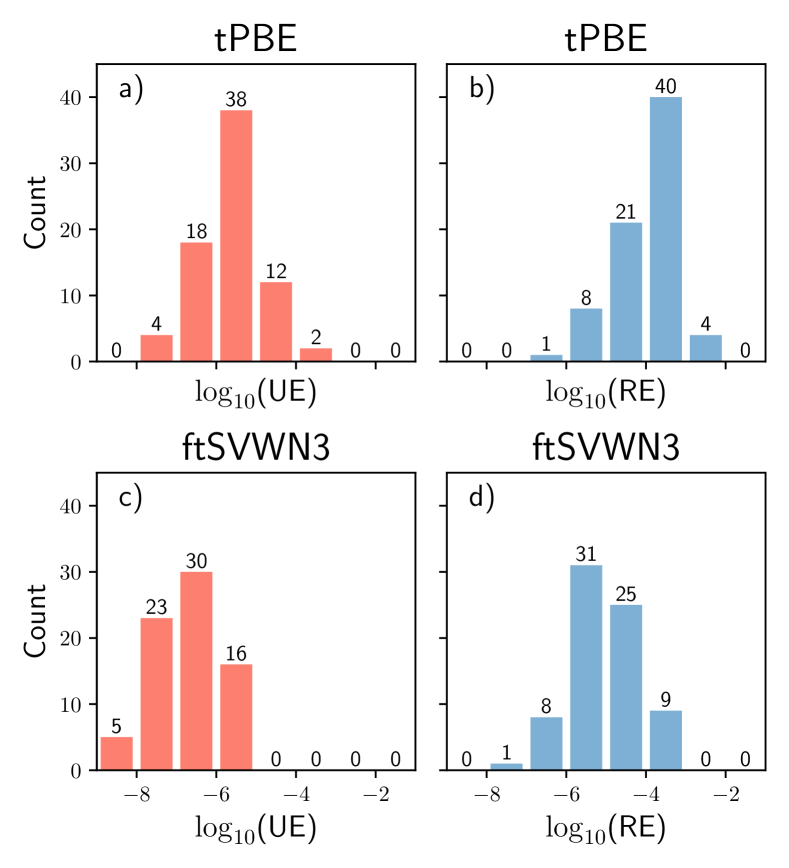
We first test our analytic gradient implementation with translated and fully-translated functionals at a variety of points on the potential energy curves of two diatomic systems: \ceHeH+ 62, 63, 64, 65, 66 and \ceLiH 67, 68, 69, 70, 71. Analytic and numerical gradients were computed for interatomic distances in the range \qtyrange0.44.0 with a step size of {0.1}. As both the common log of UE and RE occur in roughly standard distributions, we present the errors as histograms.
Figure 1: Distribution of the common log of the unsigned (a,c) and relative (b,d) error of analytic gradients relative to numerical gradients for all states of \ceHeH+ at various internuclear distances. The top row (a,b) is using the tPBE functional and bottom row (c,d) is using the ftSVWN3 functional.
\ce
HeH+ is the simplest possible system for which many terms in the programmable equations for L-PDFT analytic gradients do not vanish due to symmetry. The (\glsxtrshortue) and (\glsxtrshortre) distributions for both the tPBE and ftSVWN3 functional are shown in Fig.1. For the tPBE functional, the majority of the UEs are below {1e-5}\per whereas for the ftSVWN3 functional they are below {1e-6}\per. The RE is fairly constant throughout the potential energy curve for both functionals (Fig. S1 and S2) with the RE for tPBE being an order of magnitude greater than for ftSVWN3.
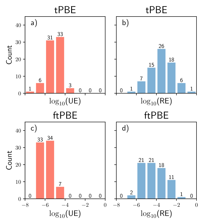
Figure 2: Distribution of the common log of the unsigned (a,c) and relative (b,d) error of analytic gradients relative to numerical gradients for all states of \ceLiH at various internuclear distances. The top row (a,b) is for the tPBE functional, and the bottom row (c,d) is for the ftPBE functional.
The (\glsxtrshortue) and (\glsxtrshortre) distributions using both the tPBE and ftPBE functionals for the lowest two 1 states of \ceLiH are summarized in Fig.2. We see that the majority of UEs are below {1e-4}\per for tPBE and below {1e-5}\per for ftPBE. There are slightly larger REs for both functionals in the dissociation region of the potential energy curve (Figs. S3 and S4) which are likely due to the flatness of the potential. For example, the largest REs for tPBE and ftPBE occur on the upper 1 state at {2.7} and {2.8} with analytic gradients of {1.7532e-3} \per and {9.0825e-5}\per respectively.
Table2 summarizes the statistical agreement between the analytic and numerical gradients for both systems and all functionals. Overall, tPBE has mean unsigned error (MUE) of {1.4e-5}\per and {2.5e-5}\per for \ceHeH+ and \ceLiH respectively; these are consistent with our previous implementations of MC-PDFT gradients. There, we saw that the analytic and numerical gradients for \ceLiH computed with tPBE and CMS-tPBE had MUEs of {4e-5}\per32 and {4.9e-5}\per61 respectively.
Table 2: Mean signed error (MSE), \glsxtrfullmue, and
root-mean-squared error (RMSE) of the analytic gradients relative to the numerical gradients. All values are in \unit\per.
\ceHeH+
\ceLiH
Functional
tPBE
ftSVWN3
tPBE
ftPBE
MSE
MUE
RMSE
The fully-translated functionals have better agreement with the numerical gradients for both \ceHeH+ and \ceLiH (Table2). This can likely be attributed to the fact that translated functionals have a discontinuity in the first derivative of the translation scheme (where values of in Eq.93 equal 1); and since L-PDFT gradients require the second derivative, this discontinuity leads to larger numerical instabilities. The fully-translated functionals, on the other hand, use a polynomial interpolation to avoid the discontinuity (AppendixA), and this likely leads to more accurate gradients.
Overall, we find good agreement between the analytic and numerical gradients at all geometries considered for both \ceHeH+ and \ceLiH using both translated and fully-translated functionals.
IV.2 Formaldehyde
Here we consider calculations with a full-valence active space of the optimized ground state () and the first excited state of character () of formaldehyde. In the ground state, formaldehyde is a planar molecule with symmetry. For the first excited state of formaldehyde, it is known that the \ceC=O double bond is elongated, and the molecule is no longer planar. We define to be the angle between the \ceH-C-H plane and the \ceC=O bond, which is a measure of the nonplanarity of the structure. We will take as our reference the experimental ground- and excited-state geometries reported by Duncan 72 and Jensen and Bunker 73 respectively.
Table 3: L-PDFT ground and first excited state bond lengths, bond angles, and out-of-plane dihedral () for formaldehyde compared with various methods. All bond lengths are in \unit and all angles are in degrees. Experimental uncertainty shown in parentheses.
The L-PDFT ground- and excited-state structural parameters are summarized in Table3, where they are compared to results obtained by other methods including MC-PDFT 32 and CASPT2 74. Both the MC-PDFT and CASPT2 calculations utilize a full-valence active space, with the MC-PDFT calculation also including two additional oxygen lone-pair orbitals. Additionally, there are results 61 from MC-PDFT and compressed multi-state PDFT (CMS-PDFT) 26 using a smaller (6,5) active space. This smaller active space was chosen using the ABC2 automatic active-space selection scheme 75 by setting the parameters , , and to 3, 2, and 0 respectively. We also include results from high-level single-reference methods computed by Budzák et al.74 including second-order algebraic diagrammatic construction (ADC(2))76, second-order coupled cluster (CC2)77, third-order coupled cluster (CC3)77, 78, and coupled cluster response method with single and double excitations and noniterative connected triple excitations from CC3 (CCSDR(3)) 79.
Relative to the experimental geometry, the L-PDFT ground-state \ceC=O bond length differs by {0.003}, the \ceC-H bond length differs by {0.002}, and the \ceH-C-H bond angle differs by (Table3). For the excited state, the L-PDFT structure has a deviation of {0.005} for the \ceC=O bond length, {0.003} for the \ceC-H bond length, and for the out-of-plane dihedral () relative to the experimental geometry (Table3). The L-PDFT \ceH-C-H bond angle agrees with the experimental value to within . L-PDFT has the most accurate and \ceH-C-H bond angle values of any of the methods presented.
Overall, for predicting the ground- and excited-state structures of formaldehyde, L-PDFT performs similarly to MC-PDFT with the slightly larger (12,12) active space and also similarly to the much more expensive CASPT2 method with the same active space.
Table 4: L-PDFT adiabatic and vertical excitations in \unit (not including vibration ZPE) for the first excited state of formaldehyde compared to reported values in the literature.
Table4 summarizes the adiabatic and vertical excitation energies calculated by L-PDFT and compares them with results from the literature. All values exclude the vibrational ZPE. We take the experimental vertical excitation energy measured by electron-impact spectroscopy as our reference 81. It is not possible to compare the adiabatic excitation energy to experiments without the vibrational ZPE. Instead, since the CC3 method is known to get within {0.03} of the extrapolated full configuration interaction for a variety of molecules 80, we take CC3 to be our reference for the adiabatic excitation energy.
Like MC-PDFT, L-PDFT overestimates the vertical excitation energy with a difference of {0.19} relative to the experimental value 81. However, this should be considered in the context that all methods presented in Table4 deviate by more than {0.1} from the experimental vertical excitation energy, which may itself have some uncertainty. The L-PDFT predicted vertical excitation energy only differs from the CC3 result by {0.02} and the much more expensive CASPT2 by {0.06}. Additionally, L-PDFT almost exactly reproduces the CC3 adiabatic excitation energy, with a slightly higher excitation energy as compared to CASPT2. Overall, L-PDFT performs similarly to CC3, MC-PDFT, and CASPT2 in predicting both the adiabatic and vertical excitation energies of formaldehyde.
Table 5: Selected L-PDFT optimized internal coordinates for the ground and excited 1Ag states of s-trans-butadiene as compared to results from other methods. All bond lengths are in \unit and all bond angles are in degrees. Experimental uncertainty shown in parentheses.
Unlike formaldehyde, s-trans-butadiene has been shown to have a strong multireference character even in its 1Ag ground state 83. Table5 summarizes the selected optimized structural parameters of the 1 and 2 1Ag states of s-trans-butadiene as calculated by L-PDFT and other multireference methods 32. All active spaces are comprised of four electrons in two orbitals and two orbitals. Our reference for the ground-state structure is the experimental geometry from Haugen et al.82, whereas for the excited-state structure we take our prior results calculated at the CASPT2(4,4) level of theory as our reference 32.
In general, L-PDFT performs similarly to both MC-PDFT and CASPT2 at predicting the equilibrium structures. For the ground state, L-PDFT deviates slightly from MC-PDFT for the \ceC-C bond length (difference of {0.007}), but still does better than CASPT2. Both L-PDFT and MC-PDFT deviate the most from the experimental \ceC=C bond length. For the excited state, L-PDFT and MC-PDFT agree on nearly every parameter except for the \ceC-C bond length where they differ by only {0.002}. Overall, L-PDFT performs similarly to both MC-PDFT and CASPT2 at predicting the ground- and excited-state structures of the challenging s-trans-butadiene molecule.
Table 6: L-PDFT adiabatic and vertical excitations in \unit (not including vibrational ZPE) for the 2 1Ag state of s-trans-butadiene compared to reported values in the literature.
The theoretical best estimate (TBE) of the vertical excitation energy of s-trans-butadiene to the 2 1Ag state is {6.39} 84. Multi-state CASPT2 85 using a (4,4) active space at the equilibrium geometry predicts a vertical excitation of {6.69} 83, {0.3} above the TBE. Table6 summarizes the adiabatic and vertical excitation energies of L-PDFT as compared to the previously computed SA-CASSCF, MC-PDFT, and CASPT2 energies using a two-state model space with a (4,4) active space 32. Although the L-PDFT vertical excitation energy differs by only {0.1} from the CASPT2 predicted adiabatic excitation energy and by only {0.01} from MC-PDFT, it overestimates the vertical excitation energy by more than {0.5} as compared to the best available estimate.
IV.4 Phenol
The photochemistry of phenol has been extensively studied as it is a prototype of the motif which is common in a variety of biomolecules and aromatic compounds 12, 86, 87, 88, 89, 90, 91, 92, 93. In the original L-PDFT paper, we studied the \ceO-H photodissociation potential energy surface and found that L-PDFT was able to correctly model the potential energy surface near the conical intersection, whereas MC-PDFT surfaces unphysically crossed 27. Our active space in this paper is the same as in our prior studies of phenol 27, 61, 26 consisting of , the pz of \ceO, and the \ceC-O and \ceO-H and orbitals.
Table 7: L-PDFT selected internal coordinates for the ground- and first excited-state of phenol compared with various methods. All bond lengths are in \unit and all angles are in degrees. The experimental uncertainty is shown in parentheses.
Selected L-PDFT optimized ground- and first excited-state internal coordinates of phenol are presented in Table7 and are compared with results from other, similar methods. Our reference for the ground- and excited-state geometries are the experimental structures determined by Larsen 94 and Spangenberg et al.95 respectively. All of the PDFT and CASSCF methods in Table7 use the same (12,11) active space. We also include results from a high-level semiempirical fit that was designed to replicate the ZPE-inclusive experimental adiabatic excitation energy 91. All of the methods in the table predict relatively similar ground-state geometries, in line with the experimentally determined geometry 94. Of interest is that the excited-state geometry optimized with MC-PDFT is nonplanar, with a substantial \ceC-C-O-H dihedral of 61. It was noted that CMS-PDFT does not suffer from this incorrect nonplanarity because it correctly incorporates the state interaction between and . L-PDFT also correctly predicts a planar excited-state geometry, in agreement with CMS-PDFT 61 and experimental results 95. This confirms that L-PDFT accounts for the state interaction as well as CMS-PDFT does. Overall, L-PDFT performs better than MC-PDFT in accurately predicting the first excited-state geometry of phenol, and the results are similar to those for CMS-PDFT and other high-level methods.
Table 8: L-PDFT adiabatic and vertical excitations in \unit (not including vibration ZPE) for the first excited state of phenol compared to reported values in the literature.
CASPT2(8,8)111Excitations calculated at the CASSCF optimized geometry.96
cc-pVDZ
CASPT2(10,10)111Excitations calculated at the CASSCF optimized geometry.97
aug(O)-AVTZ222Modified aug-cc-pVTZ basis set with extra even tempered sets of and diffuse functions on the oxygen atom.
\glsxtrshortcc2333Ground state optimized with \glsxtrshortmp2 and excited state optimized with \glsxtrshortcc2.98
aug-cc-PVDZ
\glsxtrshortmrci(10,9)111Excitations calculated at the CASSCF optimized geometry.444It is possible for the vertical excitation to be lower than the adiabatic excitation when the excitations are computed at geometries optimized at a different level of theory.99
Table 9: Selected L-PDFT ground state cytosine bond lengths (in \unit) compared with similar methods and experimental quantities. Atoms are labeled according to Fig.3.
Method
Basis Set
C1-N2
N2-C3
C3-C4
C4-C5
C5-N7
C5-N6
N6-C1
C1-O8
\glsxtrshortmud333Mean unsigned deviation from experiment.
Table 10: Selected L-PDFT ground state cytosine bond angles (in degrees) compared with similar methods and experimental quantities. Atoms are labeled according to Fig.3.
Table 11: Selected L-PDFT 2 1A excited state cytosine bond lengths (in \unit) compared with similar methods and experimental quantities. Atoms are labeled according to Fig.3.
Method
Basis Set
C1-N2
N2-C3
C3-C4
C4-C5
C5-N7
C5-N6
N6-C1
C1-O8
\glsxtrshortmud666Mean unsigned deviation from MS-CASPT2.
Table 12: Selected L-PDFT 2 1A excited state cytosine bond angles (in degrees) compared with similar methods and experimental quantities. Atoms are labeled according to Fig.3.
Table8 contains a summary of the vertical and adiabatic excitation energies of phenol as obtained by L-PDFT and other methods. As in our previous work 61, we take as our reference the high-level semiempirical fit by Zhu et al.91 for both excitation energies. We also include results from CC298 (for which the ground-state geometries are optimized at the second-order Møller-Plesset perturbation theory (MP2)103, 104), internally contracted multireference configuration interaction (MRCI)105 based on a CASSCF(10,9) wave function 99, and CASPT2 using a (8,8) 96 and (10,10) 97 active space. Both the MRCI and CASPT2 results were computed at their respective reference CASSCF optimized geometries.
L-PDFT performs similarly to the previously reported MC-PDFT results 61 and overestimates the vertical and adiabatic excitation energy relative to the reference by about {0.2}. Comparatively, CASPT2 using both an (8,8) 96 and (10,10) 97 active space underestimates the vertical and adiabatic excitation energy by more than {0.2}. The relative difference between the L-PDFT vertical and adiabatic excitation energies is {0.18} which is similar to the relative difference of {0.17} predicted by the semiempirical fit 91.
IV.5 Cytosine
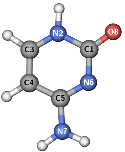
Finally, we report the optimized ground- and excited-state geometries and the adiabatic and vertical excitation energies of the nucleobase cytosine (Fig.3). Previous studies have shown that the (14,10) active space composed of five , two lone-pair, and three orbitals is sufficient for studying the low-lying excited states of cytosine 106, 107, 108.
Figure 3: Ground-state geometry of cytosine optimized with L-PDFT.
For the ground state, we take the experimental structure determined by Barker and Marsh 101 as our reference. Tables9 and 10 contain selected optimized bond lengths and angles respectively obtained from L-PDFT and other methods. All methods presented in Table9 perform similarly with a mean unsigned deviation (MUD) of {0.02} relative to the experimental bond lengths. L-PDFT performs identically to MC-PDFT for determining the cytosine bond angles with an MUD of for both methods.
Due to the lack of experimental data for the 2 1A relaxed geometry, we take the MS-CASPT2 with an (8,7) active space from the study by Nakayama et al.102 as our reference. Tables11 and 12 compares the same selected 2 1A optimized bond lengths and bond angles for L-PDFT and other methods. All methods give similar optimized bond lengths for the excited state with L-PDFT and MC-PDFT both having a MUD of {0.02}. CASPT2 and SA-CASSCF have relatively larger MUDs of {0.04} and {0.05} respectively. L-PDFT and MC-PDFT predict similar bond angles of the excited state, with L-PDFT being slightly closer to the MS-CASPT2 results with a MUD of . CASPT2 has the widest difference in the bond angles, and it overestimates the 7-5-6 bond angle by about as compared to all of the other methods.
Table 13: L-PDFT adiabatic and vertical excitations in \unit (not including vibration ZPE) for the 2 1A state of cytosine compared to reported values in the literature.
Table13 summarizes the adiabatic and vertical excitation energies for the 2 1A state of cytosine computed at various levels of theory. We take the experimental vertical excitation from Abouaf et al.110, and the MS-CASPT2(12,9) result (ground-state geometry optimized with MP2 and excited-state geometry optimized with MS-CASPT2(8,7)) as the reference for the adiabatic excitation energy Nakayama et al.102. All methods, except CC2, perform similarly with L-PDFT underestimating the reference vertical excitation energy the most. CC2 gets the closest to the experimental vertical excitation energy, differing only by {0.11}. Both L-PDFT and MC-PDFT get within {0.1} of the MS-CASPT2 adiabatic excitation energy. Overall, L-PDFT differs from MC-PDFT by only {0.03} for both the adiabatic and vertical excitation energies.
V Conclusion
We presented the derivation and implementation of analytic nuclear gradients for L-PDFT calculations based on SA-CASSCF wave functions. Because the final L-PDFT wave function is not fully variational with respect to all its parameters, we used a Lagrangian method similar to that used previously for SA-CASSCF and MC-PDFT analytic gradients. As in SA-CASSCF, we assumed equal weights to exclude the model states from the response equations. We then implemented the gradients in PySCF-forge, which is a library of PySCF extensions, and we showed that they agree with numerical gradients for both \ceHeH+ and \ceLiH using both translated and fully-translated functionals. We showed the utility of the L-PDFT analytic gradients by optimizing the ground and first excited singlet states of formaldehyde, s-trans-butadiene, phenol, and the nucleobase cytosine. Whereas MC-PDFT predicts a nonplanar first excited state of phenol, we showed that L-PDFT correctly predicts a planar structure. Additionally, we computed the vertical and adiabatic excitation energy for each molecule and saw that L-PDFT performs similarly for excitation energies to MC-PDFT and other high-level multireference methods like CASPT2.
These results are consistent with our prior study and benchmarking of L-PDFT for calculating vertical excitation energies and for modeling potential energy surfaces 29, 27. Specifically, L-PDFT correctly models the potential energy surfaces near conical intersections and locally avoided crossings whereas MC-PDFT is inaccurate 27. The results are especially encouraging because of the low cost of L-PDFT relative to MS-CASPT2 and MRCI. We conclude that L-PDFT is promising new tool for studying exited-state geometries, both vertical and adiabatic energies, photochemical reactions, and electronically nonadiabatic dynamics.
Supplementary Material
See the supplementary material associated with this article for the analytic and numerical gradients of \ceHeH+ and \ceLiH at each geometry and L-PDFT optimized structures with their corresponding energies.
Acknowledgements.
This work was supported in part by the National Science Foundation under Grant
No. CHE-2054723. M.R. Hennefarth acknowledges support by the National Science
Foundation Graduate Research Fellowship under Grant No. 2140001. We also
acknowledge the University of Chicago’s Research Computing Center for their
support of this work. Any opinion, findings, and conclusions or recommendations
expressed in this material are those of the author(s) and do not necessarily
reflect the views of the National Science Foundation.
Appendix A The Translated and Fully-Translated On-Top Functionals
Current generation on-top functionals include translated 19 or fully-translated 44KS local-spin density approximations or generalized gradient approximations functionals. These on-top functionals are defined such that
(85)
where is a KS exchange-correlation functional and are the collective translated (or fully-translated) spin-density variables and their gradients.
(86)
Here, and are effective spin densities, with primes denoting the gradient with respect to electron coordinate; and , , and being the inner product of the effective spin density gradients.
(87a)
(87b)
(87c)
For translated functionals, the following mapping is used to generate the effective spin densities and their gradients from the wave function’s density and on-top pair density:
(88)
(89)
(90)
(91)
where is given by
(92)
and is proportional to the ratio of the on-top density to the density.
(93)
Both and are functions of . Functionals translated by this scheme are simply known as ‘translated’ functionals and are given the prefix ‘t’ 19.
The above translation scheme has a discontinuity in its first derivative at . The fully-translated scheme 44 fixes this by using a polynomial interpolation to smooth out the discontinuity in the region of close to 1 as
Table 14: Parameter values for the fully-translated scheme.
Parameter
Value
can be considered a special case of with . Then, can be used to denote either or with it being clear from the context which form is being used. Consequently, the main difference between translated and fully-translated functionals is the form of and .
Appendix B SA-CASSCF Hessian in the L-PDFT Eigenstate Basis
The CI portion of the SA-CASSCF Hessian matrix, , can be expressed either in the SA-CASSCF or L-PDFT eigenstate basis. We define and as the elements of the CI Hessian in the SA-CASSCF and L-PDFT eigenstate bases respectively.
(103)
(104)
From Eq. 30 of Ref. 30, the elements of in the SA-CASSCF eigenstate basis can be written as
(105)
where are the number of states in the model space, is the real electronic Hamiltonian, and is the CASSCF energy for state .
In our implementation, we evaluate in the L-PDFT eigenstate basis. The matrices and are related to one another by the transformation matrix that rotates the SA-CASSCF states into the L-PDFT states.
(106)
Hence, we have that
(107)
where are elements of the matrix . Note that contains off-diagonal elements that most implementations of the SA-CASSCF Hessian matrix, which usually presume evaluation in the SA-CASSCF eigenstate basis, would omit.
Appendix C On-Top Gradient
The first derivative of the on-top kernel () with respect to the density variables () is obtained using the chain-rule
(108)
where is described by
(109)
(110)
and is the Jacobian matrix for the translation scheme (which has been derived previously) 31, 32.
Appendix D On-Top Hessian
The Hessian of the on-top kernel, , is generated from via the nonlinear change of variables induced by the translation scheme:
(111)
(112)
where is the first derivative of with respect to (Eq.109), is defined as the symmetric matrix (here we show only the lower triangle) of the Hessian of with respect to the translated effective spin-density variables and their gradients, is the translation Jacobian (Eq.110)31, 32, and is the Hessian of the translation. Both and are evaluated using standard KS density functional theory techniques. Specifically, in the PySCF implementation, they are evaluated using libxc. Throughout the rest of this section, we will only show the lower triangular portion of all Hessian matrices since they are symmetric.
Due to the complexity of these equations, we will instead derive the necessary equations through a serious of transformation with much more manageable Jacobians and Hessians. We will denote each set of coordinates (except the first and last corresponding to and ) as which corresponds to the variables , , , , . Correspondingly, we have that denotes the inner product between the gradient of the two variables as
(113a)
(113b)
(113c)
Furthermore, we have that the gradient and Hessian of with respect to these variables are denoted as and respectively.
(114)
(115)
Furthermore, for the transformation of to , we will let and be the corresponding Jacobian and Hessian of the transformation respectively.
The first transformation step involves going from spin-separated electron density and its derivatives to charge density () and spin density () and their derivatives. In this sense, so that we are translating as follows:
(116)
The coordinates are related by the following linear transformation:
(117)
Since this is a strictly linear transformation, we can see that can be related to the Hessian of with respect to and their gradients as
(118)
(119)
Most subsequent intermediate translation steps to the coordinates and will differ depending on whether the functional is translated or fully-translated. We first start with the simpler translated case and then go to the fully-translated case. Generally speaking though, we will undergo the following change of variables:
1.
to .
2.
to .
3.
to .
4.
to .
The Hessians are related to one another by
(120)
(121)
(122)
(123)
and the gradients are related by
(124)
(125)
(126)
(127)
All Jacobians and Hessians used for the translated functionals will be prefixed with a ‘t’ (for example, and ), and Jacobians and Hessians used for fully-translated functionals will be prefixed with an ‘ft’ (for example, and ). Once we arrive at the coordinates of , we can then change the variables to , which will be the same for translated and fully-translated functionals.
D.1 Translated On-Top Hessian
We now go to the variables by
(128)
Then
(129)
(130)
Our next transformation is to using
(131)
Note that in the translated case, there is no dependence on ; therefore, the and components do not contribute. Here, we are treating and a general function of where . Our Jacobian and Hessian for this step are
(132)
(133)
where is the second derivative of with respect to .
Next we go to the variables by the following transformation:
(134)
Again, we can omit the and variables since translated functionals do not depend on . This transformation results in
(135)
(136)
D.2 Fully-Translated On-Top Hessian
For the fully-translated case, going to the variables modifies and in Eq.128 such that
(137)
The fully-translated Jacobian and Hessian for this translation step are slight modifications of the translated matrices.
(138)
(139)
(140)
(141)
For the next transformation step to , we must include the transformations for and so that Eq.131 is modified to be
(142)
This leads to the modified Jacobian and Hessian as
(143)
(144)
(145)
(146)
where and are the Hessians of and with respect to the variables.
(147)
(148)
The final transformation we must consider separately for the fully-translated functionals is to the coordinate. Here, we must include the transformation of the and , which are not included in the translated case. The modified form of Eq.134 for the fully-translated case is thus
(149)
The fully-translated Jacobian is given by
(150)
(151)
And the fully-translated Hessian term is given by
(152)
(153)
with and the Hessian of and with respect to the variables given by
(154)
(155)
D.3 Unpacking the Sigma Vector
At this point in both the translated and fully-translated cases, we have arrived at the Hessian of with respect to , , , , and . It is fairly easy to transform to the canonical variables of by noting that
(156)
(157)
(158)
Hence, we have that
(159)
(160)
(161)
References
Grätzel 2005M. Grätzel, Solar energy conversion by dye-sensitized photovoltaic cells, Inorg. Chem. 44, 6841 (2005).
Zhugayevych and Tretiak 2015A. Zhugayevych and S. Tretiak, Theoretical description of structural and electronic properties of organic photovoltaic materials, Annu. Rev. Phys. Chem. 66, 305 (2015).
Proppe et al. 2020A. H. Proppe, Y. C. Li, A. Aspuru-Guzik, C. P. Berlinguette, C. J. Chang, R. Cogdell, A. G. Doyle, J. Flick, N. M. Gabor, R. van Grondelle, S. Hammes-Schiffer, S. A. Jaffer, S. O. Kelley, M. Leclerc, K. Leo, T. E. Mallouk, P. Narang, G. S. Schlau-Cohen, G. D. Scholes, A. Vojvodic, V. W.-W. Yam, J. Y. Yang, and E. H. Sargent, Bioinspiration in light harvesting and catalysis, Nat. Rev. Mater. 5, 828 (2020).
Croce and van Amerongen 2020R. Croce and H. van Amerongen, Light harvesting in oxygenic photosynthesis: Structural biology meets spectroscopy, Science 369, eaay2058 (2020).
McCusker 2019J. K. McCusker, Electronic structure in the transition metal block and its implications for light harvesting, Science 363, 484 (2019).
Richards et al. 2021B. S. Richards, D. Hudry, D. Busko, A. Turshatov, and I. A. Howard, Photon upconversion for photovoltaics and photocatalysis: A critical review, Chem. Rev. 121, 9165 (2021).
Wand et al. 2013A. Wand, I. Gdor, J. Zhu, M. Sheves, and S. Ruhman, Shedding new light on retinal protein photochemistry, Annu. Rev. Phys. Chem. 64, 437 (2013).
Sobolewski et al. 2002A. L. Sobolewski, W. Domcke, C. Dedonder-Lardeux, and C. Jouvet, Excited-state hydrogen detachment and hydrogen transfer driven by repulsive states: A new paradigm for nonradiative decay in aromatic biomolecules, Phys. Chem. Chem. Phys. 4, 1093 (2002).
Plasser et al. 2014F. Plasser, A. J. A. Aquino, H. Lischka, and D. Nachtigallová, Electronic excitation processes in single-strand and double-strand DNA: A computational approach, in Photoinduced Phenomena in Nucleic Acids II: DNA Fragments and Phenomenological Aspects, Topics in Current Chemistry, Vol. 356, edited by M. Barbatti, A. C. Borin, and S. Ullrich (Springer International Publishing, 2014) pp. 1–37.
Improta et al. 2016R. Improta, F. Santoro, and L. Blancafort, Quantum mechanical studies on the photophysics and the photochemistry of nucleic acids and nucleobases, Chem. Rev. 116, 3540 (2016).
Roos et al. 1980B. O. Roos, P. R. Taylor, and P. E. M. Sigbahn, A complete active space SCF method (CASSCF) using a density matrix formulated super-CI approach, Chem. Phys. 48, 157 (1980).
Roos 1987B. O. Roos, The complete active space self-consistent field method and its applications in electronic structure calculations, in Ab Initio Methods in Quantum Chemistry Part 2, Advances in Chemical Physics, Vol. 69, edited by K. P. Lawley (John Wiley & Sons, Ltd, 1987) pp. 399–445.
Andersson et al. 1990K. Andersson, P. A. Malmqvist, B. O. Roos, A. J. Sadlej, and K. Wolinski, Second-order perturbation theory with a CASSCF reference function, J. Phys. Chem. 94, 5483 (1990).
Angeli et al. 2001C. Angeli, R. Cimiraglia, S. Evangelisti, T. Leininger, and J.-P. Malrieu, Introduction of -electron valence states for multireference perturbation theory, J. Chem. Phys. 114, 10252 (2001).
Li Manni et al. 2014G. Li Manni, R. K. Carlson, S. Luo, D. Ma, J. Olsen, D. G. Truhlar, and L. Gagliardi, Multiconfiguration pair-density functional theory, J. Chem. Theory Comput. 10, 3669 (2014).
Ghosh et al. 2018S. Ghosh, P. Verma, C. J. Cramer, L. Gagliardi, and D. G. Truhlar, Combining wave function methods with density functional theory for excited states, Chem. Rev. 118, 7249 (2018).
Zhou et al. 2022C. Zhou, M. R. Hermes, D. Wu, J. J. Bao, R. Pandharkar, D. S. King, D. Zhang, T. R. Scott, A. O. Lykhin, L. Gagliardi, and D. G. Truhlar, Electronic structure of strongly correlated systems: recent developments in multiconfiguration pair-density functional theory and multiconfiguration nonclassical-energy functional theory, Chem. Sci. 13, 7685 (2022).
Hoyer et al. 2016C. E. Hoyer, S. Ghosh, D. G. Truhlar, and L. Gagliardi, Multiconfiguration pair-density functional theory is as accurate as CASPT2 for electronic excitation, J. Phys. Chem. Lett. 7, 586 (2016).
King et al. 2022D. S. King, M. R. Hermes, D. G. Truhlar, and L. Gagliardi, Large-scale benchmarking of multireference vertical-excitation calculations via automated active-space selection, J. Chem. Theory Comput. 18, 6065 (2022).
Sand et al. 2018aA. M. Sand, C. E. Hoyer, D. G. Truhlar, and L. Gagliardi, State-interaction pair-density functional theory, J. Chem. Phys. 149, 024106 (2018a).
Bao et al. 2020aJ. J. Bao, C. Zhou, Z. Varga, S. Kanchanakungwankul, L. Gagliardi, and D. G. Truhlar, Multi-state pair-density functional theory, Faraday Discuss. 224, 348 (2020a), 2003.06744v2 .
Hennefarth et al. 2023aM. R. Hennefarth, M. R. Hermes, D. G. Truhlar, and L. Gagliardi, Linearized pair-density functional theory, J. Chem. Theory Comput. 19, 3172 (2023a).
Granovsky 2011A. A. Granovsky, Extended multi-configuration quasi-degenerate perturbation theory: The new approach to multi-state multi-reference perturbation theory, J. Chem. Phys. 134, 214113 (2011).
Hennefarth et al. 2023bM. R. Hennefarth, D. S. King, and L. Gagliardi, Linearized pair-density functional theory for vertical excitation energies, J. Chem. Theory Comput. 19, 7983 (2023b).
Stålring et al. 2001J. Stålring, A. Bernhardsson, and R. Lindh, Analytical gradients of a state average MCSCF state and a state average diagnostic, Mol. Phys. 99, 103 (2001).
Sand et al. 2018bA. M. Sand, C. E. Hoyer, K. Sharkas, K. M. Kidder, R. Lindh, D. G. Truhlar, and L. Gagliardi, Analytic gradients for complete active space pair-density functional theory, J. Chem. Theory Comput. 14, 126 (2018b), 1709.04985 .
Scott et al. 2020T. R. Scott, M. R. Hermes, A. M. Sand, M. S. Oakley, D. G. Truhlar, and L. Gagliardi, Analytic gradients for state-averaged multiconfiguration pair-density functional theory, J. Chem. Phys. 153, 1 (2020).
Scott et al. 2021T. R. Scott, M. S. Oakley, M. R. Hermes, A. M. Sand, R. Lindh, D. G. Truhlar, and L. Gagliardi, Analytic gradients for multiconfiguration pair-density functional theory with density fitting: Development and application to geometry optimization in the ground and excited states, J. Chem. Phys. 154, 074108 (2021).
Hellmann 1933H. Hellmann, Zur rolle der kinetischen elektronenenergie für die zwischenatomaren kräfte, Z. Phys 85, 180 (1933).
Hellmann 1937H. Hellmann, Einführung in die quantenchemie (Franz Deuticke, Leipzig und Wien, 1937).
Press et al. 1992W. H. Press, S. A. Teukolsky, W. T. Vetterling, and B. P. Flannery, Numerical recipes in Fortran 77: the art of scientific computing, 2nd ed., Vol. 2 (Cambridge: Cambridge University Press, Cambridge, 1992).
Bernhardsson et al. 1999A. Bernhardsson, R. Lindh, J. Olsen, and M. Fulscher, A direct implementation of the second-order derivatives of multiconfigurational SCF energies and an analysis of the preconditioning in the associated response equation, Mol. Phys. 96, 617 (1999).
Helgaker et al. 2014T. Helgaker, P. Jørgensen, and J. Olsen, Molecular electronic-structure theory (Wiley, Hoboken, 2014).
Helgaker and Almlöf 1984T. U. Helgaker and J. Almlöf, A second‐quantization approach to the analytical evaluation of response properties for perturbation‐dependent basis sets, Int. J. Quantum Chem. 26, 275 (1984).
Löwdin 1950P.-O. Löwdin, On the non-orthogonality problem connected with the use of atomic wave functions in the theory of molecules and crystals, J. Chem. Phys. 18, 365 (1950).
Dunning 1989T. H. Dunning, Gaussian basis sets for use in correlated molecular calculations. I. the atoms boron through neon and hydrogen, J. Chem. Phys. 90, 1007 (1989).
Perdew et al. 1996J. P. Perdew, K. Burke, and M. Ernzerhof, Generalized gradient approximation made simple, Phys. Rev. Lett. 77, 3865 (1996).
Carlson et al. 2015R. K. Carlson, D. G. Truhlar, and L. Gagliardi, Multiconfiguration pair-density functional theory: A fully translated gradient approximation and its performance for transition metal dimers and the spectroscopy of Re2Cl82–, J. Chem. Theory Comput. 11, 4077 (2015).
Bloch 1929F. Bloch, Bemerkung zur elektronentheorie des ferromagnetismus und der elektrischen leitfähigkeit, Z. Phys. 57, 545 (1929).
Vosko et al. 1980S. H. Vosko, L. Wilk, and M. Nusair, Accurate spin-dependent electron liquid correlation energies for local spin density calculations: a critical analysis, Can. J. Phys. 58, 1200 (1980).
Kendall et al. 1992R. A. Kendall, T. H. Dunning, and R. J. Harrison, Electron affinities of the first-row atoms revisited. systematic basis sets and wave functions, J. Chem. Phys. 96, 6796 (1992).
Feller 1996D. Feller, The role of databases in support of computational chemistry calculations, J. Comput. Chem. 17, 1571 (1996).
Schuchardt et al. 2007K. L. Schuchardt, B. T. Didier, T. Elsethagen, L. Sun, V. Gurumoorthi, J. Chase, J. Li, and T. L. Windus, Basis set exchange: A community database for computational sciences, J. Chem. Inf. Model. 47, 1045 (2007).
Papajak and Truhlar 2010E. Papajak and D. G. Truhlar, Convergent partially augmented basis sets for post-Hartree-Fock calculations of molecular properties and reaction barrier heights, J. Chem. Theory Comput. 7, 10 (2010).
Celani and Werner 2003P. Celani and H.-J. Werner, Analytical energy gradients for internally contracted second-order multireference perturbation theory, J. Chem. Phys. 119, 5044 (2003).
Sun et al. 2017Q. Sun, T. C. Berkelbach, N. S. Blunt, G. H. Booth, S. Guo, Z. Li, J. Liu, J. D. McClain, E. R. Sayfutyarova, S. Sharma, S. Wouters, and G. K. Chan, PySCF: The Python-based simulations of chemistry framework, WIREs Comput. Mol. Sci. 8, e1340 (2017), 1701.08223 .
Sun et al. 2020Q. Sun, X. Zhang, S. Banerjee, P. Bao, M. Barbry, N. S. Blunt, N. A. Bogdanov, G. H. Booth, J. Chen, Z.-H. Cui, J. J. Eriksen, Y. Gao, S. Guo, J. Hermann, M. R. Hermes, K. Koh,
P. Koval, S. Lehtola, Z. Li, J. Liu, N. Mardirossian, J. D. McClain, M. Motta, B. Mussard, H. Q. Pham, A. Pulkin, W. Purwanto, P. J. Robinson, E. Ronca, E. R. Sayfutyarova, M. Scheurer, H. F. Schurkus,
J. E. T. Smith, C. Sun, S.-N. Sun, S. Upadhyay, L. K. Wagner, X. Wang, A. White, J. D. Whitfield, M. J. Williamson, S. Wouters, J. Yang, J. M. Yu, T. Zhu, T. C. Berkelbach, S. Sharma, A. Y. Sokolov, and G. K.-L. Chan, Recent developments in the PySCF program package, J. Chem. Phys. 153, 024109 (2020), 2002.12531 .
Marques et al. 2012M. A. L. Marques, M. J. T. Oliveira, and T. Burnus, libxc: A library of exchange and correlation functionals for density functional theory, Comput. Phys. Commun. 183, 2272 (2012), 1203.1739 .
Lehtola et al. 2018S. Lehtola, C. Steigemann, M. J. Oliveira, and M. A. Marques, Recent developments in libxc — a comprehensive library of functionals for density functional theory, SoftwareX 7, 1 (2018).
Wang and Song 2016L.-P. Wang and C. Song, Geometry optimization made simple with translation and rotation coordinates, J. Chem. Phys. 144, 214108 (2016).
Bao et al. 2022J. J. Bao, M. R. Hermes, T. R. Scott, A. M. Sand, R. Lindh, L. Gagliardi, and D. G. Truhlar, Analytic gradients for compressed multistate pair-density functional theory, Mol. Phys. 120, e2110534 (2022).
Peyerimhoff 1965S. Peyerimhoff, Hartree—Fock—Roothaan wavefunctions, potential curves, and charge-density contours for the HeH + (X1+) and NeH+(X 1+) molecule ions, J. Chem. Phys. 43, 998 (1965).
Güsten et al. 2019R. Güsten, H. Wiesemeyer, D. Neufeld, K. M. Menten, U. U. Graf, K. Jacobs, B. Klein, O. Ricken, C. Risacher, and J. Stutzki, Astrophysical detection of the helium hydride ion HeH +, Nature 568, 357 (2019).
Novotný et al. 2019O. Novotný, P. Wilhelm, D. Paul, Á. Kálosi, S. Saurabh, A. Becker, K. Blaum, S. George, J. Göck, M. Grieser, F. Grussie, R. von Hahn, C. Krantz, H. Kreckel, C. Meyer, P. M. Mishra, D. Muell, F. Nuesslein, D. A. Orlov, M. Rimmler, V. C. Schmidt, A. Shornikov, A. S. Terekhov, S. Vogel, D. Zajfman, and A. Wolf, Quantum-state–selective electron recombination studies suggest enhanced abundance of primordial HeH+, Science 365, 676 (2019).
Fallon et al. 1960R. J. Fallon, J. T. Vanderslice, and E. A. Mason, Potential energy curves for lithium hydride, J. Chem. Phys. 32, 1453 (1960).
Li and Stwalley 1978K. C. Li and W. C. Stwalley, The A1+ X1+ bands of the isotopic lithium hydrides, J. Mol. Spectrosc. 69, 294 (1978).
Pardo et al. 1986A. Pardo, J. Camacho, and J. Poyato, The Padé-approximant method and its applications in the construction of potential-energy curves for the lithium hydride molecule, Chem. Phys. Lett. 131, 490 (1986).
Stwalley and Zemke 1993W. C. Stwalley and W. T. Zemke, Spectroscopy and structure of the lithium hydride diatomic molecules and ions, J. Phys. Chem. Ref. Data 22, 87 (1993).
Tung et al. 2011W.-C. Tung, M. Pavanello, and L. Adamowicz, Very accurate potential energy curve of the LiH molecule, J. Chem. Phys. 134, 064117 (2011).
Duncan 1974J. L. Duncan, The ground-state average and equilibrium structures of formaldehyde and ethylene, Mol. Phys. 28, 1177 (1974).
Jensen and Bunker 1982P. Jensen and P. R. Bunker, The geometry and the inversion potential function of formaldehyde in the Ã1A2 and ã 3A2 electronic states, J. Mol. Spectrosc. 94, 114 (1982).
Budzák et al. 2017Š. Budzák, G. Scalmani, and D. Jacquemin, Accurate excited-state geometries: a CASPT2 and coupled-cluster reference database for small molecules, J. Chem. Theory Comput. 13, 6237 (2017).
Bao and Truhlar 2019J. J. Bao and D. G. Truhlar, Automatic active space selection for calculating electronic excitation energies based on high-spin unrestricted hartree–fock orbitals, J. Chem. Theory Comput. 15, 5308 (2019).
Dreuw and Wormit 2014A. Dreuw and M. Wormit, The algebraic diagrammatic construction scheme for the polarization propagator for the calculation of excited states, WIREs Comput. Mol. Sci. 5, 82 (2014).
Christiansen et al. 1995O. Christiansen, H. Koch, and P. Jørgensen, The second-order approximate coupled cluster singles and doubles model CC2, Chem. Phys. Lett. 243, 409 (1995).
Koch et al. 1997H. Koch, O. Christiansen, P. Jørgensen, A. M. Sanchez de Merás, and T. Helgaker, The CC3 model: An iterative coupled cluster approach including connected triples, J. Chem. Phys. 106, 1808 (1997).
Christiansen et al. 1996O. Christiansen, H. Koch, and P. Jørgensen, Perturbative triple excitation corrections to coupled cluster singles and doubles excitation energies, J. Chem. Phys. 105, 1451 (1996).
Loos et al. 2018P.-F. Loos, A. Scemama, A. Blondel, Y. Garniron, M. Caffarel, and D. Jacquemin, A mountaineering strategy to excited states: highly accurate reference energies and benchmarks, J. Chem. Theory Comput. 14, 4360 (2018), 1807.02045 .
Walzl et al. 1987K. N. Walzl, C. F. Koerting, and A. Kuppermann, Electron-impact spectroscopy of acetaldehyde, J. Chem. Phys. 87, 3796 (1987).
Haugen et al. 1966W. Haugen, M. Trætteberg, F. Kaufmann, K. Motzfeldt, D. H. Williams, E. Bunnenberg, C. Djerassi, and R. Records, The molecular structure of 1,3-butadiene and 1,3,5-trans-hexatriene., Acta Chem. Scand. 20, 1726 (1966).
Shu and Truhlar 2017Y. Shu and D. G. Truhlar, Doubly excited character or static correlation of the reference state in the controversial 2 1Ag state of trans-butadiene?, J. Am. Chem. Soc. 139, 13770 (2017).
Watson and Chan 2012M. A. Watson and G. K.-L. Chan, Excited states of butadiene to chemical accuracy: reconciling theory and experiment, J. Chem. Theory Comput. 8, 4013 (2012).
Finley et al. 1998J. Finley, P.-Å. Malmqvist, B. O. Roos, and L. Serrano-Andrés, The multi-state CASPT2 method, Chem. Phys. Lett. 288, 299 (1998).
Ashfold et al. 2006M. N. R. Ashfold, B. Cronin, A. L. Devine, R. N. Dixon, and M. G. D. Nix, The role of * excited states in the photodissociation of heteroaromatic molecules, Science 312, 1637 (2006).
Devine et al. 2008A. L. Devine, M. G. D. Nix, R. N. Dixon, and M. N. R. Ashfold, Near-ultraviolet photodissociation of thiophenol, J. Phys. Chem. A 112, 9563 (2008).
Ashfold et al. 2008M. N. R. Ashfold, A. L. Devine, R. N. Dixon, G. A. King, M. G. . D. Nix, and T. A. A. Oliver, Exploring nuclear motion through conical intersections in the UV photodissociation of phenols and thiophenol, Proc. Natl. Acad. Sci. 105, 12701 (2008).
Lim et al. 2009J. S. Lim, H. Choi, I. S. Lim, S. B. Park, Y. S. Lee, and S. K. Kim, Photodissociation dynamics of thiophenol-d1: the nature of excited electronic states along the S-D bond dissociation coordinate, J. Phys. Chem. A 113, 10410 (2009).
Xu et al. 2013X. Xu, K. R. Yang, and D. G. Truhlar, Diabatic molecular orbitals, potential energies, and potential energy surface couplings by the 4-fold way for photodissociation of phenol, J. Chem. Theory Comput. 9, 3612 (2013).
Zhu et al. 2016X. Zhu, C. L. Malbon, and D. R. Yarkony, An improved quasi-diabatic representation of the 1, 2, 3 1A coupled adiabatic potential energy surfaces of phenol in the full 33 internal coordinates, J. Chem. Phys. 144, 124312 (2016).
Zhang et al. 2018L. Zhang, D. G. Truhlar, and S. Sun, Electronic spectrum and characterization of diabatic potential energy surfaces for thiophenol, Phys. Chem. Chem. Phys. 20, 28144 (2018).
Zhang et al. 2019L. Zhang, D. G. Truhlar, and S. Sun, Full-dimensional three-state potential energy surfaces and state couplings for photodissociation of thiophenol, J. Chem. Phys. 151, 154306 (2019).
Larsen 1979N. W. Larsen, Microwave spectra of the six mono-13 C-substituted phenols and of some monodeuterated species of phenol. Complete substitution structure and absolute dipole moment, J. Mol. Struct. 51, 175 (1979).
Spangenberg et al. 2003D. Spangenberg, P. Imhof, and K. Kleinermanns, The S1 state geometry of phenol determined by simultaneous Franck–Condon and rotational constants fits, Phys. Chem. Chem. Phys. 5, 2505 (2003).
Granucci et al. 2000G. Granucci, J. T. Hynes, P. Millié, and T.-H. Tran-Thi, A theoretical investigation of excited-state acidity of phenol and cyanophenols, J. Am. Chem. Soc. 122, 12243 (2000).
Dixon et al. 2011R. N. Dixon, T. A. A. Oliver, and M. N. R. Ashfold, Tunnelling under a conical intersection: Application to the product vibrational state distributions in the UV photodissociation of phenols, J. Chem. Phys. 134, 194303 (2011).
Pino et al. 2010G. A. Pino, A. N. Oldani, E. Marceca, M. Fujii, S.-I. Ishiuchi, M. Miyazaki, M. Broquier, C. Dedonder, and C. Jouvet, Excited state hydrogen transfer dynamics in substituted phenols and their complexes with ammonia: - energy gap propensity and ortho-substitution effect, J. Chem. Phys. 133, 124313 (2010).
Vieuxmaire et al. 2008O. P. J. Vieuxmaire, Z. Lan, A. L. Sobolewski, and W. Domcke, Ab initio characterization of the conical intersections involved in the photochemistry of phenol, J. Chem. Phys. 129, 224307 (2008).
Fogarasi 2002G. Fogarasi, Relative stabilities of three low-energy tautomers of cytosine: a coupled cluster electron correlation study, J. Phys. Chem. A 106, 1381 (2002).
Nakayama et al. 2014A. Nakayama, S. Yamazaki, and T. Taketsugu, Quantum chemical investigations on the nonradiative deactivation pathways of cytosine derivatives, J. Phys. Chem. A 118, 9429 (2014).
Møller and Plesset 1934Chr. Møller and M. S. Plesset, Note on an approximation treatment for many-electron systems, Phys. Rev. 46, 618 (1934).
Head-Gordon et al. 1988M. Head-Gordon, J. A. Pople, and M. J. Frisch, MP2 energy evaluation by direct methods, Chem. Phys. Lett. 153, 503 (1988).
Knowles and Werner 1992P. J. Knowles and H.-J. Werner, Internally contracted multiconfiguration-reference configuration interaction calculations for excited states, Theoret. Chim. Acta 84, 95 (1992).
Merchán et al. 2006M. Merchán, R. González-Luque, T. Climent, L. Serrano-Andrés, E. Rodríguez, M. Reguero, and D. Peláez, Unified model for the ultrafast decay of pyrimidine nucleobases, J. Phys. Chem. B 110, 26471 (2006).
González-Vázquez and González 2010J. González-Vázquez and L. González, A time-dependent picture of the ultrafast deactivation of keto-cytosine including three-state conical intersections, ChemPhysChem 11, 3617 (2010).
Nakayama et al. 2013A. Nakayama, Y. Harabuchi, S. Yamazaki, and T. Taketsugu, Photophysics of cytosine tautomers: new insights into the nonradiative decay mechanisms from MS-CASPT2 potential energy calculations and excited-state molecular dynamics simulations, Phys. Chem. Chem. Phys. 15, 12322 (2013).
Cherneva et al. 2023T. D. Cherneva, M. M. Todorova, R. I. Bakalska, I. G. Shterev, E. Horkel, and V. B. Delchev, Experimental and theoretical study of the cytosine tautomerism through excited states, J. Mol. Model. 29, 303 (2023).
Abouaf et al. 2004R. Abouaf, J. Pommier, H. Dunet, P. Quan, P.-C. Nam, and M. T. Nguyen, The triplet state of cytosine and its derivatives: Electron impact and quantum chemical study, J. Chem. Phys. 121, 11668 (2004).
![[Uncaptioned image]](/html/2401.12933/assets/x4.png)