Viability and control of a delayed SIR epidemic
with an ICU State Constraint

Abstract.

This paper studies viability and control synthesis for a delayed SIR epidemic. The model integrates a constant delay representing an incubation/latency time. The control inputs model non-pharmaceutical interventions, while an intensive care unit (ICU) state-constraint is introduced to reflect the healthcare system’s capacity. The arising delayed control system is analyzed via functional viability tools, providing insights into fulfilling the ICU constraint through feedback control maps. In particular, we consider two scenarios: first, we consider the case of general continuous initial conditions. Then, as a further refinement of our analysis, we assume that the initial conditions satisfy a Lipschitz continuity property, consistent with the considered model. The study compares the (in general, sub-optimal) obtained control policies with the optimal ones for the delay-free case, emphasizing the impact of the delay parameter. The obtained results are supported and illustrated, in a concluding section, by numerical examples.

Keywords: SIR epidemic; state constraints; viability; optimal control; feedback control; delays; functional differential equations.

2020 Mathematics Subject Classification: 34K35, 49J21, 49J53, 92D30, 93C23.

1. Introduction

The optimal control of epidemics (see, for instance [2, 6, 21, 31]) starting from the classical SIR model of Kermack and McKendrick ([25]), has been widely studied in recent years, also because of the COVID-19 pandemic, see [1, 5, 17, 26, 27]. In this paper, we focus on the viability analysis and the synthesis of control strategies for the following two-dimensional SIR model with delay:

$$\begin{cases}\dfrac{ds}{dt}(t)=-b(t)\,s(t)\,i(t-h)\\[8.61108pt] \dfrac{di}{dt}(t)=b(t)\,s(t)\,i(t-h)-\gamma i(t).\\[8.61108pt] \end{cases}$$ (1.1)

Here $h>0$ is a given positive number representing a constant delay, modeling the presence of an incubation/latency time, i.e., assuming a temporal gap between the disease contraction and the development of infectivity of average individuals. The parameter $\gamma\in(0,1)$ represents the natural (and constant) recovery rate, while the control parameters are measurable functions $b(t)\in U:=[\beta_{\star},\beta]$ for some $0<\beta_{\star}\leq\beta<1$. The value $\beta$ models the natural transmission rate of the disease, while $\beta_{\star}$ represents the minimal attainable transmission rate obtained via non-pharmaceutical policies (social distancing, lockdowns, etc.) The initial conditions are imposed by prescribing a pair of continuous functions $\phi=(i_{\phi},s_{\phi}):[-h,0]\to\mathbb{R}^{2}$, and by requiring that

$$i(t)=i_{\phi}(t) s(t)=s_{\phi}(t) t\in[-h,0]$$ and for all . (1.2)

The derivatives in (1.1) are meant in a distributional sense and the trajectories are constructed from admissible controls $b\in\mathcal{U}:=L^{\infty}((0,+\infty);U)$.

The delayed version (1.1) of the classical Kermack and McKendrick SIR model [25], with a constant trasmission rate coefficient $b\equiv\beta$, was introduced in [11, 7]. This model has been widely studied, from the stability point of view, in several papers, as for instance [43, 32]. Optimization and optimal control problems have been more recently considered in [44] but always in the case of a constant transmission rate. In [7], the nonnegative constant $h$ represents a time during which the infectious agents develop in a vector and it is only after time $h$ that the infected vector can infect a susceptible individual. On the other hand, $h$ can also be regarded as a latency time only after which the infected individual becomes able to transmit the infection. In this slightly different interpretation, system (1.1) has been considered in the recent Covid-19 studies [29] and [41] but, in the latter, with a constant transmission rate $b\equiv\beta$. We mention [42, 34] among the recent studies about the impact of a latency period on Covid-19 transmission.

We consider system (1.1) under an intensive care unit (ICU) constraint on the number of infected (cft. [24, 33, 4]), i.e., we require that

$$i(t)\leq i_{M}\;\;\forall\,t\geq 0,$$ (1.3)

for some fixed $0<i_{M}\leq 1$. In this setting, the prescribed level $i_{M}$ represents an upper bound to the capacity of the health-care system to treat infected patients.

From a theoretical point of view, the delay system (1.1) together with the constraint (1.3) can be seen as a differential delayed inclusion, as defined in [18, 22, 14]. Within this approach, the analysis of (1.1)-(1.3) can be tackled by using the functional viability tools introduced in [19] and well summarized in [3, Chapter 12]. For recent developments in this area see, for example, [13, 12]. Functional viability analysis provides geometric characterizations of the notions of uncontrolled forward invariance and viability (i.e., the property of being forward invariant under a suitable control). Under some technical restrictions, these ideas allow us to provide an explicit state-space description of subsets of initial conditions for which the constraint (1.3) is satisfied by solutions to (1.1), under arbitrary or suitable controls actions.

Viability analysis, as said, implicitly highlights feasible control actions which allow to keep the solutions of (1.1) in the feasible region (defined by the constraint (1.3)). Consequently, it also provides selection mechanisms for implementing such control actions, in the form of feedback control maps. This selection procedure can also be tuned according to the minimization of a given cost functional of the form

$$\int_{0}^{+\infty}G(\beta-b(t))\,dt,$$ (1.4)

where $G$ is a continuous and strictly increasing scalar function. Thus, summarizing, the performed viability analysis allows us to provide a (in general, sub-optimal) feedback strategy, which depends only on the current and past position of the state, for the optimal control problem (1.1)-(1.3)-(1.4). We formally compare our viability results with those obtained in the delay-free case (see [4, 16]), which can be recovered by taking the limit as $h\to 0$.

We point out that different approaches to the study of delayed optimal control problems have been proposed in the literature. Notably, we underline that recent researches studied various formulations of Pontryagin principles for delayed optimal control problems with state constraints, see [38, 39, 8] and references therein. The arising conditions are necessary for optimality of feasible control polices and rely on an advance-differential equation governing the adjoint states. On the other hand, differently from the delay-free case studied in [15, 4, 16], these Pontryagin-principle-based conditions have, up to now and for the problem under consideration, been unable to provide exact closed-form expression for the optimal control policy. On the other hand, viability analysis provides itself a satisfactory alternative and a flexible tool in building feedback control polices that only depends on the present and past values of the solutions.

The paper is organized as follows. In Section 2 we introduce the main notation and definitions. We also provide a self-contained summary of viability analysis tools for delayed differential inclusions, basically borrowed from [19, 3], together with a novel characterization result for some particular class of (functional) subsets. In Section 3 we provide a preliminary qualitative analysis of system (1.1), comparing and underlying the peculiarities of this model with respect to the delay-free case. In Section 4 we provide the applications of viability analysis for system (1.1) under the state-constraint (1.3); considering two cases.

1. First, we consider initial conditions as general continuous functions $\phi:[-h,0]\to\mathbb{R}^{2}$, satisfying the ICU constraint (1.3), and provide a complete viability analysis and the corresponding feedback control policy.

2. We then strengthen our hypothesis, supposing that initial conditions also satisfy a Lipschitz property compatible with the considered model. In this setting, we prove that when the delay converges to $0$ we are able to recover the viable regions of the delay-free case studied in [4, 16].

In Section 5 we illustrate our results with the aid of numerical examples, and some concluding remarks are provided in Section 6. Some technical proofs are postponed in a final Appendix, to avoid breaking the flow of the presentation.

Notation:

We denote by $\mathbb{R}_{+}=[0,+\infty)$ the set of non-negative reals. Given $A\subset\mathbb{R}^{n}$ and $B\subset\mathbb{R}^{m}$, we denote by $\mathcal{C}(A;B)$ and $\mathcal{C}^{1}(A;B)$ the set of continuous and continuously differentiable functions from $A$ to $B$, respectively. Given $x\in\mathbb{R}^{n}$, the scalar $|x|$ is its Euclidean norm. Given two sets $A,B$, the notation $g:A\rightsquigarrow B$ stands for the set-valued map $g:A\to\mathcal{P}(B)$ where $\mathcal{P}(B)$ is the power set of $B$. Given a norm $\|\cdot\|$ on $\mathbb{R}^{n}$, and $R>0$, denote by $B_{\|\cdot\|}(0,R)$ the closed ball (w.r.t. $\|\cdot\|$) of radius $R$. Given $v,w\in\mathbb{R}^{n}$, $\langle v,w\rangle\in\mathbb{R}$ denotes the Euclidean scalar product of $v$ and $w$. Given $x\in\mathbb{R}^{n}$, we denote by $|x|_{\max}:=\max\{|x_{1}|,|x_{2}|,\dots,|x_{n}|\}$ its max (or infinity) norm.

2. Notation and Preliminaries

2.1. The delayed SIR model: notation and existence of solutions

Let us consider the delay system introduced in (1.1) with state constraint (1.3). Besides those already given in the introduction, we use the following notation: $x:=(s,i)\in\mathbb{R}^{2}$, $\mathcal{C}:=\mathcal{C}([-h,0];\mathbb{R}^{2})$. Moreover, the components of a given $\phi\in\mathcal{C}$ will be denoted by $s_{\phi}$ and $i_{\phi}$, that is, $\phi(t)=(s_{\phi}(t),i_{\phi}(t))$ for all $t\in[-h,0]$. Let us define $f:\mathcal{C}\times U\to\mathbb{R}^{2}$ by

$$f(\phi,b):=\left(-bs_{\phi}(0)i_{\phi}(-h),\ bs_{\phi}(0)i_{\phi}(-h)-\gamma i_{\phi}(0)\right),$$ (2.1)

and introduce the set-valued map $F_{U}:\mathcal{C}\rightsquigarrow\mathbb{R}^{2}$ defined by

$$F_{U}(\phi):=\{f(\phi,b)\ |\ b\in[\beta_{\star},\beta]\}.$$ (2.2)

It can be seen that $F_{U}$ has convex and compact values, it is locally bounded and upper semicontinuous (we refer to [35, 3] for these general concepts).

For any $t\in\mathbb{R}$, consider the map

$$S(t):\mathcal{C}(\mathbb{R};\mathbb{R}^{2})\to \ \mathcal{C}$$ (2.3)

$$x\mapsto \ S(t)x$$

$$\ [S(t)x](s):=x(t+s)\;\;\forall\,s\in[-h,0].$$

In the delay-systems community, the simplified notation $S(t)x:=x_{t}$ is often used. As the control changes in the space $\mathcal{U}$, the class of Cauchy problems (1.1)-(1.2) can thus be rewritten as a delayed differential inclusion of the form

$$\begin{cases}x^{\prime}(t)\in F_{U}(S(t)x),\\ S(0)x=\phi\in\mathcal{C}.\end{cases}$$ (2.4)

According to [18], a solution to (2.4) is a continuous function $x_{\phi}:[-h,\tau)\to\mathbb{R}^{2}$, with $\tau>0$, satisfying (2.4) for almost all $t\in[0,\tau)$ an such that $x_{\phi}$ is absolutely continuous on every compact subinterval of $[0,\tau)$. As done for the initial condition, the two components of $x_{\phi}$ will be denoted by $s_{\phi}$ and $i_{\phi}$, that is, $x_{\phi}(t)=(s_{\phi}(t),i_{\phi}(t))$ for all $t\in[-h,\tau)$. This is consistent with the fact that $x_{\phi}(t)=\phi(t)$ whenever $t\in[-h,0]$.

As a preliminary result, we show that, for a remarkable class of initial conditions, solutions exist and are globally defined.

Let us define the triangle

$$T:=\{x\in\mathbb{R}^{2}\ |\ s\geq 0,\ i\geq 0,\ s+i\leq 1\}$$

and introduce the set $\mathcal{T}:=\mathcal{C}([-h,0];T)$.

Lemma 2.1.

For any initial condition $\phi\in\mathcal{T}$ and for any control input $b\in\mathcal{U}$, there exists a unique solution $x_{\phi}:[-h,+\infty)\to\mathbb{R}^{2}$ to the Cauchy problem (1.1)-(1.2). Moreover, $x_{\phi}(t)\in T$ for every $t\in[-h,+\infty)$. We will denote this solution also with $x_{\phi,b}$ (or $x^{\phi,b}$), when we want to stress the fact that it corresponds to the prescribed input $b$.

Proof.

Given any $\phi\in\mathcal{T}$ and any $b\in\mathcal{U}$, the local existence and uniqueness of the solution follows by [20, Chapter 2, Subsection 2.6]. Let us denote by $x_{\phi}:[-h,\tau)\to\mathbb{R}^{2}$, $\tau>0$, such solution and prove that $x_{\phi}(t)=(s_{\phi,b}(t),i_{\phi}(t))\in T$ for all $t\in[0,\tau)$. First we note that, by considering $i_{\phi}:[-h,\tau)\to\mathbb{R}$ as a coefficient and integrating the first equation in (1.1), we have

$$s_{\phi}(t)=s_{\phi}(0)e^{\int_{0}^{t}b(r)i_{\phi}(r-h)\,dr}.$$

Since $s_{\phi}(0)\geq 0$ by hypothesis, this implies that $s_{\phi}(t)\geq 0$ for all $t\in[0,\tau)$. Using also the non-negativity of the initial condition, we get

$$i^{\prime}_{\phi}(t)=b(t)s_{\phi}(t)i_{\phi}(t-h)-\gamma i_{\phi}(t)\geq-\gamma i_{\phi}(t)\;\;\forall\,t\in[0,h)\cap[0,\tau).$$

By a comparison argument (see for example [37, Lemma 1.2]), the previous inequality implies

$$i_{\phi}(t)\geq i_{\phi}(0)e^{-\gamma t}\geq 0\;\;\forall\,t\in[0,h)\cap[0,\tau).$$

By iterating the argument on any interval of the form $[kh,(k+1)h]$ for $k\in\mathbb{N}$, we conclude that $i_{\phi}(t)\geq 0$ for all $t\in[0,\tau)$. Now, summing the equations in (1.1) we have

$$(s_{\phi}(t)+i_{\phi}(t))^{\prime}=-\gamma i_{\phi}(t)\;\;\forall t\in[0,\tau).$$

Since, by assumption, $i_{\phi}(0)+s_{\phi}(0)\leq 1$, this implies that $s_{\phi}(t)+i_{\phi}(t)\leq 1$ for all $t\in[0,\tau)$. We have thus proved that if $\phi\in\mathcal{T}$, then $x_{\phi}(t)\in T$, for all $t\in[0,\tau)$. Since $T$ is compact, the results in [20, Theorem 3.1 and Subsection 2.6, Chapter 2,] imply that the solution exists in $[0,+\infty)$, and the proof is concluded. ∎

Well-posedness results, like that of Lemma 2.1, can be found also in [11] for the constant control case and in  [43, 32] for slightly different delayed SIR models. We note that the proof substantially shows that any triangle of the form $\{x\in\mathbb{R}_{+}^{2}\;|\;s+i\leq a\}$ for $a\geq 0$ is invariant. It is physically reasonable to consider initial conditions in $\mathcal{T}$, as $s_{\phi}(t)$ and $i_{\phi}(t)$ are the fractions of susceptible (resp. infectious) population at time $t$. Thus, the preliminary Lemma 2.1 can be seen as a permanence result: if the initial condition is a “physically feasible” curve, the solution, forward in time, remains in the region of physical feasibility, no matter the external input $b\in\mathcal{U}$.

2.2. Viability for delay systems: general theory and first results.

We recall here the definitions of viability/forward invariance for delay systems and related results ([3, Chapter 12], [19]). Given any dimension $n\in\mathbb{N}$, consider a set valued map $F:\mathcal{C}([-h,0];\mathbb{R}^{n})\rightsquigarrow\mathbb{R}^{n}$ (in this subsection, we write $\mathcal{C}=\mathcal{C}([-h,0];\mathbb{R}^{n})$) and a delayed differential inclusion of the form

$$\begin{cases}x^{\prime}(t)\in F(S(t)x),\\ S(0)x=\phi\in\mathcal{C}.\end{cases}$$ (2.5)

For the SIR model (1.1) we “a priori” know that solutions exist and are globally defined, for suitable initial conditions and controls, as proved in Lemma 2.1. For this reason and to simplify the notation, in this subsection we suppose that for any $\phi\in\mathcal{C}$ the solution set of (2.5) is non-empty and maximal solutions are defined on $\mathbb{R}_{+}$.

Definition 2.2.

Given $\mathcal{K}\subseteq\mathcal{C}$, we say that

1. $\mathcal{K}$ is forward invariant for (2.5) if for any $\phi\in\mathcal{K}$ and any solution $x_{\phi}$ to (2.5), starting at $\phi$, we have $S(t)x_{\phi}\in\mathcal{K}$ for all $t\in\mathbb{R}_{+}$;

2. $\mathcal{K}$ is viable for (2.5) if for any $\phi\in\mathcal{K}$ there exists a solution $x_{\phi}$ to (2.5), starting at $\phi$, for which it holds that $S(t)x_{\phi}\in\mathcal{K}$ for all $t\in\mathbb{R}_{+}$.

The following concept of feasible directions (see [3, Definition 12.2.1]) is useful in providing a geometric characterization of forward invariance and viability.

Definition 2.3.

Given a subset $\mathcal{K}\subseteq\mathcal{C}$ and $\phi\in\mathcal{K}$, the set of feasible directions to $\mathcal{K}$ at $\phi$ is defined by

$$D_{\mathcal{K}}(\phi):=\big{\{}v\in\mathbb{R}^{n}\!\!\!\!\! :\!\!\!\! \forall\,\varepsilon>0,\ \exists\,\tau\in(0,\varepsilon)\ \text{and}\ \phi_{\tau}\in\mathcal{C}(\mathbb{R},\mathbb{R}^{n})\ \text{such that}$$ (2.6)

$$S(0)\phi_{\tau}=\phi,\ S(\tau)\phi_{\tau}\in\mathcal{K},\ \frac{\phi_{\tau}(\tau)-\phi_{\tau}(0)}{\tau}\in B(v,\varepsilon)\big{\}},$$

where $B(v,\varepsilon)$ denotes the closed ball of $\mathbb{R}^{n}$ with radius $\varepsilon$ and centered in $v$.

In our setting, a more concise representation of the set of feasible directions can be given in terms of the classical notion of Bouligand contingent cone, recalled below.

Definition 2.4.

Consider $K\subset\mathbb{R}^{n}$ and $x\in K$, the Bouligand contingent cone to $K$ at $x$ is defined by

$$T_{K}(x):=\{v\in\mathbb{R}^{n}\ |\ \exists\,t_{k}\to 0,t_{k}>0,\ \exists\,v_{k}\to v\text{ such that }x+t_{k}v_{k}\in K\ \forall\,k\in\mathbb{N}\}.$$

It is well-known that, if the set $K$ is convex, the Bouligand contigent cone coincides with the classical tangent cone of convex analysis, i.e.,

$$T_{K}(x)=\text{cl}\left(\{v\in\mathbb{R}^{n}\ |\ \exists\,\lambda\geq 0\text{ and }\exists\,y\in K\text{ such that }v=\lambda(y-x)\}\right),$$

see [35, Theorem 6.9]. If $x\in\text{int}(K)$, then $T_{K}(x)=\mathbb{R}^{n}$. Moreover, if the convex set $K\subset\mathbb{R}^{n}$ is defined by

$$K=\{x\in\mathbb{R}^{n}\ |\ g_{i}(x)\leq 0,\,i\in\{1,\dots,M\}\},$$ (2.7)

for some $g_{1},\dots,g_{M}\in\mathcal{C}^{1}(\mathbb{R}^{n};\mathbb{R})$, then, for any $x\in\partial K$ such that $g_{i}(x)=0$ for all $i\in I\subseteq\{1,\dots,M\}$ (and $g_{j}(x)\neq 0$ for $j\notin I$), we have

$$T_{K}(x)=\{v\in\mathbb{R}^{n}\ |\ \langle\nabla g_{i}(x),v\rangle\leq 0\ \forall\,i\in I\},$$ (2.8)

see [35, Theorem 6.31].

In the sequel, the subset $\mathcal{K}\subset\mathcal{C}$ will represent the set of initial conditions of the epidemic model (1.1). As anticipated in the Introduction, we are going to consider two different kinds of initial conditions, sharing the same set $K\subseteq S\subseteq\mathbb{R}^{n}$ of traces in $0$. First, we take the subset $\mathcal{K}_{S}\subset\mathcal{C}$ defined by

$$\mathcal{K}_{S}=\{\phi\in\mathcal{C}\ |\ \phi(0)\in K,\,\phi(t)\in S\ \forall\,t\in[-h,0]\}.$$ (2.9)

Besides this large set, we consider the following smaller sets of Lipschitz continuous initial conditions, i.e., given a constant $L>0$, we take

$$\mathcal{K}_{S,L}=\{\phi\in\mathcal{C}_{L,\|\cdot\|}\ |\ \phi(0)\in K,\,\phi(t)\in S\ \forall\,t\in[-h,0]\},$$ (2.10)

where $\mathcal{C}_{L,\|\cdot\|}$ denotes the set of functions $\phi\in\mathcal{C}$ that are $L$-Lipschitz in $[-h,0]$ w.r.t. the norm $\|\cdot\|$ in $\mathbb{R}^{n}$, i.e., $\|\phi(t_{1})-\phi(t_{2})\|\leq L|t_{1}-t_{2}|$, for all $t_{1},t_{2}\in[-h,0]$. In the following statement we characterize the set of feasible directions of Definition 2.3 for these different choices of initial conditions.

Lemma 2.5.

Consider a set $K\subset\mathbb{R}^{n}$ and a convex set $S\supseteq K$. The following characterization of the set of feasible directions to $\mathcal{K}_{S}$ in (2.9) holds:

$$D_{\mathcal{K}_{S}}(\phi)=T_{K}(\phi(0))\;\;\,\forall\phi\in\mathcal{K}_{S}.$$ (2.11)

Moreover, given $L>0$, we have

$$D_{\mathcal{K}_{S,L}}(\phi)=T_{K}(\phi(0))\cap B_{\|\cdot\|}(0,L)\;\;\,\forall\,\phi\in\mathcal{K}_{S,L}.$$ (2.12)

Proof.

First of all, we note that given $x\in K$ we have

$$T_{K}(x)=\{v\in\mathbb{R}^{n}\ |\ \exists\,t_{k}\to 0,\,t_{k}>0,\,v_{k}\to v\text{ such that }\|v_{k}\|=\|v\|\text{ and }x+t_{k}v_{k}\in K\ \forall\,k\in\mathbb{N}\},$$ (2.13)

i.e., we can add, without loss of generality, the constraint $\|v_{k}\|=\|v\|$ to the sequences of vectors in Definition 2.4. Indeed, this is clear if $v=0\in T_{K}(x)$. When, instead, $0\neq v\in T_{K}(x)$, starting from some sequences $t_{k}>0$ and $v_{k}\in\mathbb{R}^{n}\setminus\{0\}$ such that $t_{k}\to 0$, $v_{k}\to v$ and $x+t_{k}v_{k}\in K$, $\forall k\in\mathbb{N}$, the claim is proved by taking the modified sequences $\widetilde{t}_{k}=\frac{\|v_{k}\|}{\|v\|}t_{k}$ and $\widetilde{v}_{k}=\frac{\|v\|}{\|v_{k}\|}v_{k}$.
Let us note, moreover, that it is enough to prove (2.12), since the proof of (2.11) can be easily obtained from the latter, by sending $L$ to $+\infty$.

Given $\phi\in\mathcal{K}_{S,L}$, let us start by proving the inclusion $T_{K}(\phi(0))\cap B_{\|\cdot\|}(0,L)\subseteq D_{\mathcal{K}_{S,L}}(\phi)$. For $v\in T_{K}(\phi(0))\cap B_{\|\cdot\|}(0,L)$, let $t_{k}$ and $v_{k}$ be two sequences as in (2.13). Given any $\varepsilon>0$ consider a $k\in\mathbb{N}$ large enough such that $t_{k}<\varepsilon$ and $\|v_{k}-v\|<\varepsilon$. Define $\tau=t_{k}$ and consider $\psi\in\mathcal{C}([0,\tau],\mathbb{R}^{n})$ defined by $\psi(s)=\phi(0)+sv_{k}$ for any $s\in[0,\tau]$. By convexity of $S$, $\psi(s)\in S$ for all $s\in[0,\tau]$. Moreover, $\psi$ is $L$-Lipschitz, since $\|\psi^{\prime}(s)\|=\|v_{k}\|=\|v\|\leq L$, for any $s\in[0,\tau]$. We then define $\phi_{\tau}=\phi\ast\psi\in\mathcal{C}([-h,\tau],\mathbb{R}^{n})$, where $\ast$ denotes the concatenation in time. To prove that $v\in\mathcal{D}_{\mathcal{K}_{L,S}}(\phi)$ we have to verify that $\phi_{\tau}$ satisfies the conditions (2.6) of Definition 2.3, with $\mathcal{K}=\mathcal{K}_{S,L}$. We trivially have $S(0)\phi_{\tau}=\phi$ and, moreover, $S(\tau)\phi_{\tau}(0)=\phi_{\tau}(\tau)=\phi(0)+t_{k}v_{k}\in K$. We also note that $S(\tau)\phi_{\tau}(s)\in S$ for all $s\in[-h,0]$ and that $S(\tau)\phi_{\tau}$ is $L$-Lipschitz. We have thus proved that $S(\tau)\phi_{\tau}\in\mathcal{K}_{S,L}$. Also the remaining condition in  (2.6) holds since

$$\frac{\phi_{\tau}(\tau)-\phi_{\tau}(0)}{\tau}=\frac{\phi(0)+t_{k}v_{k}-\psi(0)}{t_{k}}=v_{k}\in B_{\|\cdot\|}(v,\varepsilon),$$

thus concluding the proof of the claimed inclusion.
We now prove the opposite inclusion, $\mathcal{D}_{\mathcal{K}_{S,L}}(\phi)\subseteq T_{K}(\phi(0))\cap B_{\|\cdot\|}(0,L)$. Given any $v\in\mathcal{D}_{\mathcal{K}_{L,S}}(\phi)$ and any $k\in\mathbb{N}$, consider $\varepsilon=\frac{1}{k}$, $\tau\in(0,\varepsilon)$ and $\psi_{\tau}$ as in Definition 2.3. Define $t_{k}=\tau$ and $v_{k}=\frac{\psi_{\tau}(\tau)-\psi_{\tau}(0)}{\tau}$. By definition of $\mathcal{K}_{S,L}$, we have

$$\|v_{k}\|=\frac{\|\psi_{\tau}(\tau)-\psi_{\tau}(0)\|}{\tau}\leq\frac{L\tau}{\tau}=L.$$

To conclude, we recall that $t_{k}\leq\frac{1}{k}\to 0$ and $v_{k}\to v$ and thus $\|v\|\leq L$. Hence $v\in T_{K}(\phi(0))\cap B_{\|\cdot\|}(0,L)$, and the proof is concluded. ∎

Remark 2.6.

We note that in Lemma 2.5 we have proven, in particular, that the sets $\mathcal{D}_{\mathcal{K}_{S}}(\phi)$ and $\mathcal{D}_{\mathcal{K}_{S},L}(\phi)$ are independent of the set $S$, which constrains the past values of the initial conditions. Indeed, $\mathcal{D}_{\mathcal{K}_{S}}(\phi)$ and $\mathcal{D}_{\mathcal{K}_{S},L}(\phi)$ only depends on the “arrival” set $K$ and on the final position $\phi(0)$ (and on the Lipschitz constant $L>0$, in the case of $\mathcal{D}_{\mathcal{K}_{S},L}(\phi)$). This property, which holds for sets of the form (2.9) and (2.10), is crucial in the subsequent analysis.

In the next statement we specialize the main result concerning viability theory, namely Theorem 12.2.2 [3], to the case in which the set $\mathcal{K}$ is of the form (2.9) or (2.10).

Theorem 2.7.

Consider a set-valued map $F:\mathcal{C}\rightsquigarrow\mathbb{R}^{n}$ which is upper semicontinuous with nonempty, convex and compact values. Given compact and convex sets $K\subseteq S\subset\mathbb{R}^{n}$, and $L>0$, a set $\mathcal{K}\subset\mathcal{C}$ of the form (2.9) or (2.10) is forward invariant for (2.5) (resp.  viable) if and only if

$$\;F(\phi)\subseteq D_{\mathcal{K}}(\phi)\,\;\forall\;\phi\in\mathcal{K},$$

(resp.) $$F(\phi)\cap D_{\mathcal{K}}(\phi)\neq\varnothing\;\,\forall\;\phi\in\mathcal{K}.$$

Proof.

For the case $\mathcal{K}$ of the form (2.9), we apply [18, Corollary 1.1], recalling by Lemma 2.5 that $\mathcal{D}_{\mathcal{K}}(\phi)=T_{K}(\phi(0))$ for all $\phi\in\mathcal{K}$.

In the case $\mathcal{K}$ defined as in (2.10) it suffices to apply Theorem 12.2.2 in [3], after having observed that the closedness of $K$ in $\mathbb{R}^{n}$ implies that $\mathcal{K}$ is closed with respect to the norm of uniform convergence. ∎

In spite of the fact that the sets of feasible directions are independent of $S$, the characterization of invariant (resp. viable) sets, in fact, depend on the past, since the conditions of Theorem 2.7 must by verified on the $(S,L)$-depending set $\mathcal{K}$ of initial conditions. As a consequence, when the set $S\subseteq\mathbb{R}^{n}$ is fixed in (2.9) and (2.10), a notion of maximality of the set $K$ (of the traces $\phi(0)$ of the initial conditions $\phi\in\mathcal{K}$) cannot neglect the past behavior of the functions $\phi$. We thus give now an appropriate definition which distinguishes between initial conditions in $\mathcal{K}_{S}$ and $\mathcal{K}_{S,L}$.

Definition 2.8.

Consider a set $\mathcal{H}\subseteq\mathcal{C}$, a set $S\subseteq\mathbb{R}^{n}$ and an upper semicontinuous set-valued map $F:\mathcal{C}\rightsquigarrow\mathbb{R}^{n}$ with nonempty, convex and compact values. A set $K\subseteq S$ is said to be

• the maximal forward invariant set with $\mathcal{H}$-past in $S$ for (2.5) if $K$ is the largest set such that

  $$\mathcal{K}:=\{\phi\in\mathcal{H}\ |\ \phi(0)\in K,\ \phi(s)\in S\ \forall s\in[-h,0]\}$$

  is forward invariant (in the sense of Definition 2.2).

• the maximal viable set with $\mathcal{H}$-past in $S$ for (2.5) if $K$ is the largest set such that

  $$\mathcal{K}:=\{\phi\in\mathcal{H}\ |\ \phi(0)\in K,\ \phi(s)\in S\ \forall s\in[-h,0]\}$$

  is viable (in the sense of Definition 2.2).

When $\mathcal{H}=\mathcal{C}$ the $\mathcal{H}$-prefix is dropped.

2.3. Viability for the delayed SIR model

For the set-valued map $F_{U}:\mathcal{C}([-h,0],\mathbb{R}^{2})\rightsquigarrow\mathbb{R}^{2}$ of the delayed SIR model introduced in (2.2), Theorem 2.7 specializes in the following statement.

Corollary 2.9.

Given compact and convex sets $K\subseteq S\subset\mathbb{R}^{2}$ and $L>0$, a set $\mathcal{K}\subset\mathcal{C}([-h,0],\mathbb{R}^{2})$ of the form (2.9) or (2.10) is forward invariant (resp. viable) for (2.4) if and only if

$$f(\phi,b)\in D_{\mathcal{K}}(\phi)\ \forall\,\phi\in\mathcal{K}\ \forall\,b\in[\beta_{\star},\beta],\;\,$$

(resp.) $$\forall\,\phi\in\mathcal{K},\ \exists\,b\in[\beta_{\star},\beta]\,:\,f(\phi,b)\in D_{\mathcal{K}}(\phi).$$

3. Qualitative Analysis of Solutions

In this section we collect some properties of (solutions to) system (2.4) under arbitrary inputs $b\in\mathcal{U}$.

By Lemma 2.1, we have that for every initial condition $\phi\in\mathcal{T}$ a solution to the Cauchy problem for (2.4) exists and its values belong to $T$. Our aim is now to study the asymptotic behavior of such solutions.

First, we note that the case in which $\phi=(s_{\phi},i_{\phi})\in\mathcal{T}$ is such that $i_{\phi}(t)=0$ for every $t\in[-h,0]$ is not physically relevant. Nevertheless it is trivial, since in this case $(s_{\phi}(t),i_{\phi}(t))\equiv(s_{\phi}(0),0)$ for all $t\in\mathbb{R}_{+}$. For this reason, in the rest of this section we assume that

$$i_{\phi}\not\equiv 0 [-h,0]$$ in . (3.1)

Let us call $\mathcal{T}_{0}$ the set of all $\phi\in\mathcal{T}$ satisfying (3.1).

Our first result is inspired by [11], in which the case of a constant $b(t)$ is treated; here we adapt the argument to the time-varying case.

Lemma 3.1.

Consider any control input $b\in\mathcal{U}$, and any $\phi\in\mathcal{T}_{0}$. Then, $s_{\phi}$ is non-increasing in $[0,+\infty)$, and it holds that

$$\lim_{t\to+\infty}i_{\phi}(t)=0,\;\;\;\lim_{t\to+\infty}s_{\phi}(t)=s_{\phi,\infty}\in[0,\frac{\gamma}{\beta_{\star}}),$$

where $s_{\phi,\infty}$ depends only on $b$, $\phi(0)$ and $\int_{-h}^{0}i_{\phi}(\tau)\;d\tau$.

Moreover,

1. if $s_{\phi}(0)>0$, then

   1. $s_{\phi,\infty}>0$,

   2. $i_{\phi}(t)>0$ for all $t\geq h$,

   3. $s_{\phi}$ is strictly decreasing in $[2h,+\infty)$;

2. if the input $b$ is eventually essentially constant, i.e., if there exist $T>0$ and $b_{\infty}\in[\beta_{\star},\beta]$ such that $b(t)=b_{\infty}$ for almost all $t\in[T,+\infty)$, then $s_{\phi,\infty}<\frac{\gamma}{\,b_{\infty}}$.

Proof.

For every $\phi\in\mathcal{T}_{0}$, $s_{\phi}(\cdot):\mathbb{R}_{+}\to\mathbb{R}_{+}$ is non-increasing since, by the invariance of $\mathcal{T}$ stated in Lemma 2.1, we have $s^{\prime}_{\phi}(t)\leq 0$ for all $t\in\mathbb{R}_{+}$. Moreover, $s_{\phi}(\cdot)$ is bounded from below by $0$ and thus the limit

$$\lim_{t\to+\infty}s_{\phi}(t)=:s_{\phi,\infty}$$

exists and belongs to $[0,1]$. Define $N_{\phi}(t):=s_{\phi}(t)+i_{\phi}(t)$. We have that

$$N^{\prime}_{\phi}(t)=-\gamma i_{\phi}(t),\ t\in\mathbb{R}_{+},$$ (3.2)

and thus also $N_{\phi}(t)$ is a non-increasing function and admits a non-negative limit, by Lemma 2.1. Since $i_{\phi}(t)=N_{\phi}(t)-s_{\phi}(t)$, also $i_{\phi}$ admits a limit $i_{\phi,\infty}$, which is non-negative again by Lemma 2.1.

On the other hand, by integrating (3.2) on a time interval $[T,+\infty)$ with $T\geq 0$, and using that $i_{\phi,\infty}\geq 0$, we get

$$\int_{T}^{\infty}i_{\phi}(\tau)\;d\,\tau=\frac{N_{\phi}(T)-s_{\phi,\infty}-i_{\phi,\infty}}{\gamma}\leq\frac{N_{\phi}(T)-s_{\phi,\infty}}{\gamma}.$$ (3.3)

From the last inequality we immediately get that $i_{\phi,\infty}=\lim_{t\to\infty}i_{\phi}(t)=0$, and the first equality in (3.3) becomes

$$\int_{T}^{\infty}i_{\phi}(\tau)\;d\,\tau=\frac{N_{\phi}(T)-s_{\phi,\infty}}{\gamma}\ \mbox{ for every }T\geq 0.$$ (3.4)

To conclude the proof of the first part of the statement, it remains to show that $s_{\phi,\infty}<\frac{\gamma}{\beta_{\star}}$.

We use here the notation $b(t)=\beta_{\star}+v(t)$ with $v\in L^{\infty}(\mathbb{R}_{+};[0,\beta-\beta_{\star}])$. By integrating the first equation in (1.1) for $t\geq h$, and performing a simple change of variable, we obtain

$$s_{\phi}(t) =s_{\phi}(0)\,\text{exp}\left(-\int_{0}^{t}b(\tau)i_{\phi}(\tau-h)\;d\tau\right)$$

$$=s_{\phi}(0)\,\text{exp}\left(-\int_{-h}^{0}b(\tau+h)i_{\phi}(\tau)\;d\tau-\beta_{\star}\int_{0}^{t-h}i_{\phi}(\tau)\,d\tau-\int_{0}^{t-h}v(\tau+h)i_{\phi}(\tau)\;d\tau\right).$$

As $t\to+\infty$, we have

$$s_{\phi,\infty}=s_{\phi}(0)\,\text{exp}\left(-\int_{-h}^{0}b(\tau+h)i_{\phi}(\tau)\;d\tau-\beta_{\star}\int_{0}^{\infty}i_{\phi}(\tau)\,d\tau-\int_{0}^{\infty}v(\tau+h)i_{\phi}(\tau)\;d\tau\right).$$ (3.5)

By using the equation (3.4) with $T=0$ to substitute the integral $\int_{0}^{\infty}i_{\phi}(\tau)\,d\tau$ in (3.5), we obtain

$$s_{\phi,\infty}=s_{\phi}(0)\,\text{exp}\left(-\int_{-h}^{0}b(\tau+h)i_{\phi}(\tau)\;d\tau-\int_{0}^{\infty}v(\tau+h)i_{\phi}(\tau)\;d\tau-\frac{\beta_{\star}}{\gamma}(N_{\phi}(0)-s_{\phi,\infty})\right).$$ (3.6)

Equation (3.6) can be written in the equivalent form

$$s_{\phi,\infty}e^{-\frac{\beta_{\star}}{\gamma}s_{\phi,\infty}}=M(\phi,b)s_{\phi}(0)e^{-\frac{\beta_{\star}}{\gamma}s_{\phi}(0)}$$ (3.7)

with

$$M(\phi,b):=\text{exp}\left(-\int_{-h}^{0}b(\tau+h)i_{\phi}(\tau)\;d\tau-\int_{0}^{\infty}v(\tau+h)i_{\phi}(\tau)\;d\tau-\frac{\beta_{\star}}{\gamma}(i_{\phi}(0))\right).$$

Since $i_{\phi}(t)$ is not identically zero in $[-h,0]$ then $M(\phi,b)<1$. By this inequality and (3.7), then we get

$$s_{\phi,\infty}e^{-\frac{\beta_{\star}}{\gamma}s_{\phi,\infty}}<s_{\phi}(0)e^{-\frac{\beta_{\star}}{\gamma}s_{\phi}(0)}$$ (3.8)

Let us now introduce the function $g(z):=ze^{-\frac{\beta_{\star}}{\gamma}z}$, which is increasing in $[0,\frac{\gamma}{\beta_{\star}}]$ and decreasing in $[\frac{\gamma}{\beta_{\star}},+\infty)$. If $s_{\phi}(0)<\frac{\gamma}{\beta_{\star}}$ then the claim ($s_{\phi,\infty}<\frac{\gamma}{\beta_{\star}}$) follows by the monotonicity of $s_{\phi}$. Let us consider then the case $s_{\phi}(0)\geq\frac{\gamma}{\beta_{\star}}$ and assume by contradiction that $s_{\phi,\infty}\geq\frac{\gamma}{\beta_{\star}}$. Since $s_{\phi,\infty}\leq s_{\phi}(0)$, by the monotonicity of $g$ in the interval $[\frac{\gamma}{\beta_{\star}},+\infty)$ we have $g(s_{\phi,\infty})\geq g(s_{\phi}(0))$, so contradicting (3.8). This completes the proof of the first part of the statement.

Let us now start proving the “moreover” part (1) of the statement.

If $s_{\phi}(0)>0$, from (3.7), we have $s_{\phi,\infty}>0$, that is (1)(a).

To prove (1)(b), we first show that there exists a $\tau\in[0,h]$ such that $i_{\phi}(\tau)>0$. Since $i_{\phi}$ is continuous and not identically zero in $[-h,0]$, there exist $\delta\in(0,h)$ and $\varepsilon>0$ such that $i_{\phi}(s)>0$ for all $s\in(-h+\delta-\varepsilon,-h+\delta)$. Since $s_{\phi}(0)>0$, we have already proven that $s_{\phi}(t)\geq s_{\phi_{\infty}}>0$ for all $t\in\mathbb{R}_{+}$. Suppose by contradiction that $i_{\phi}(s)=0$, for all $s\in[0,\delta]$. We have

$$i_{\phi}(\delta)=\int_{0}^{\delta}b(s)s_{\phi}(s)i_{\phi}(s-h)\,ds\geq\beta_{\star}s_{\phi,\infty}\int_{0}^{\delta}i_{\phi}(s-h)\,ds\geq\beta_{\star}s_{\phi,\infty}\int_{-h+\delta-\varepsilon}^{-h+\delta}i_{\phi}(s)\,ds>0,$$

leading to a contradiction. We can thus fix $\tau\in[0,h]$, such that $i_{\phi}(\tau)>0$. Since $i_{\phi}^{\prime}(t)\geq-\gamma i_{\phi}(t)$, by the comparison principle (see [37, Lemma 1.1]) it holds that

$$i_{\phi}(t)\geq i_{\phi}(\tau)e^{-\gamma(t-\tau)},$$ (3.9)

thus proving that $i_{\phi}(t)>0$ for all $t\geq h$, that is (1)(b).

Assertion 1(c) is a direct consequence of (1)(a) and (1)(b), because $s_{\phi}(t)=-b(t)s_{\phi}(t)i_{\phi}(t-h)<0$ if $t\geq 2h$.

Let us now prove (2). Suppose that there exists $T>h$ and $b_{\infty}\in[\beta_{\star},\beta]$ such that $b(t)=b_{\infty}$, for almost all $t\in[T,+\infty)$. By integrating the first equation of (1.1) on the interval $[T,t]$ for a $t\geq T+h$, we obtain

$$s_{\phi}(t) =s_{\phi}(T)\,\text{exp}\left(-\int_{T}^{t}b(\tau)i_{\phi}(\tau-h)\;d\tau\right)=s_{\phi}(T)\,\text{exp}\left(-b_{\infty}\int_{T-h}^{T}i_{\phi}(\tau)\;d\tau-b_{\infty}\int_{T}^{t-h}i_{\phi}(\tau)\,d\tau\right).$$

By taking the limit as $t\to+\infty$, we have

$$s_{\phi,\infty}=s_{\phi}(T)\,\text{exp}\left(-b_{\infty}\int_{T-h}^{T}i_{\phi}(\tau)\;d\tau-b_{\infty}\int_{T}^{\infty}i_{\phi}(\tau)\,d\tau\right).$$ (3.10)

By using the equation (3.4) to substitute the integral $\int_{T}^{\infty}i_{\phi}(\tau)\,d\tau$ in (3.10), and manipulating, we see that $s_{\phi,\infty}$ satisfies the equation

$$s_{\phi,\infty}e^{-\frac{b_{\infty}}{\gamma}s_{\phi,\infty}}=M_{T}(\phi,b_{\infty})s_{\phi}(T)e^{-\frac{b_{\infty}}{\gamma}s_{\phi}(T)}$$ (3.11)

with

$$M_{T}(\phi,b_{\infty}):=\text{exp}\left(-b_{\infty}\int_{T-h}^{T}i_{\phi}(\tau)\;d\tau-\frac{b_{\infty}}{\gamma}(i_{\phi}(T))\right)<1,$$

since by (1)(b) if $i_{\phi}(t)$ is not identically zero in $[-h,0]$, then $i_{\phi}(T)>0$. Recalling that $s_{\phi,\infty}\leq s_{\phi}(T)$, and arguing as in the proof of the first part of the statement we see that (3.11) implies $s_{\phi,\infty}<\frac{\gamma}{b_{\infty}}$. ∎

In the delay-free case, i.e., when $h=0$ the value $s=\frac{\gamma}{\beta}$ is the herd immunity threshold, see for example [4, 16] and references therein. In this case, if $s_{\phi}(0)\leq\frac{\gamma}{\beta}$ and $i_{\phi}(0)>0$, (1.1) immediately implies that $i_{\phi}:\mathbb{R}_{+}\to\mathbb{R}$ is strictly decreasing. In the subsequent statement we show that $\frac{\gamma}{\beta}$ is an important threshold also in the delay case (when $h>0$): if at the current instant the susceptible population $s$ is smaller than this value, the number of infected people $i$ will not exceed again the maximum value attained in the last $h$-period of time.

Lemma 3.2.

Consider any control input $b\in\mathcal{U}$. Given any $\phi\in\mathcal{T}_{0}$ and any $\tau\in\mathbb{R}_{+}$, define $\widehat{\imath}\,(\phi,\tau):=\displaystyle\max_{t\in[\tau-h,\tau]}i_{\phi}(t)$. Then, for any $\phi\in\mathcal{T}_{0}$ such that $s_{\phi}(0)\leq\frac{\gamma}{\beta}$, we have

$$i_{\phi}(t+\tau)\leq\widehat{\imath}\,(\phi,\tau),\;\;\forall\,\tau\in\mathbb{R}_{+}\ \forall\,t\in[0,h].$$ (3.12)

Proof.

Consider any $\tau\in\mathbb{R}_{+}$, and suppose by contradiction that there exists a $\bar{\tau}\in[\tau,\tau+h]$ such that $i_{\phi}(\bar{\tau})>\widehat{\imath}\,(\phi,\tau)$. Consider

$$\tau_{1}=\max\{t\in[\tau,\bar{\tau}]\ :\ i_{\phi}(t)=\widehat{\imath}\,(\phi,\tau)\},$$

which exists by continuity and because $i_{\phi}(\tau)\leq\widehat{\imath}\,(\phi,\tau)$ and $i_{\phi}(\bar{\tau})>\widehat{\imath}\,(\phi,\tau)$. Moreover, $\tau_{1}<\bar{\tau}$. Then, by definition of $\tau_{1}$, it holds that $i_{\phi}(t)\geq\widehat{\imath}\,(\phi,\tau)$ for all $t\in[\tau_{1},\bar{\tau}]$. We have

$$i_{\phi}(\bar{\tau})=i_{\phi}(\tau_{1})+\int_{\tau_{1}}^{\bar{\tau}}b(t)s_{\phi}(t)i_{\phi}(t-h)-\gamma i_{\phi}(t)\,dt\leq\widehat{\imath}(\phi,\tau)+\gamma\int_{\tau_{1}}^{\bar{\tau}}(i_{\phi}(t-h)-\widehat{\imath}\,(\phi,\tau))\,dt\leq\widehat{\imath}\,(\phi,\tau),$$

where, in the last inequality, we used that $i_{\phi}(t-h)\leq\widehat{\imath}\,(\phi,\tau)$ for all $t\in[\tau_{1},\bar{\tau}]$ because $t-h\in[\tau-h,\tau]$, and that $s_{\phi}(t)\leq s_{\phi}(0)\leq\frac{\gamma}{\beta}$, for all $t\geq 0$. This leads to a contradiction which concludes the proof. ∎

In Lemma 3.2, rephrasing, we have proved that, for any $\phi\in\mathcal{T}_{0}$ such that $s_{\phi}(0)\leq\frac{\gamma}{\beta}$, the function $t\mapsto\|S(t)i_{\phi}\|_{\infty}=\max_{s\in[0,h]}i_{\phi}(t-s)$ is non-increasing. This should be compared with the delay-free case (see [4, 16]), in which, if the initial condition $(s_{\phi}(0),i_{\phi}(0))$ is such that $s_{\phi}(0)\leq\frac{\gamma}{\beta}$ and $i_{\phi}(0)>0$, we have that the function $t\mapsto i_{\phi}(t)$ is strictly decreasing. In this regard, Lemma 3.2 provides a “weak” decreasing property of the infectious component $i_{\phi}$ of the state in the delay case. We want to stress the fact that, when $h>0$, (3.12) does not imply that $i_{\phi}$ be monotonic (which, in fact, might be not).

4. Viability analysis and control

Given a parameter $0<i_{M}\leq 1$ (representing the maximal acceptable proportion of infected), we are going to analyze the cases in which the trajectories of (1.1)/(2.4) stay (can be forced to be in) the feasible set

$$C:=\{x\in T\;|\;i\leq i_{M}\}.$$ (4.1)

4.1. Arbitrary feasible initial conditions

In this subsection we consider the case in which the controller has a limited knowledge on the past evolution of the epidemics: we suppose that it is only known that in the past $h$ time-units, the value of $i_{\phi}$ did not exceed the safety threshold $i_{M}$. More formally, we will assume the following.

Assumption 4.1.

The initial condition $\phi\in\mathcal{C}$ satisfies $\phi(t)\in C$ for all $t\in[-h,0]$.

We now need to introduce some additional state-space curves, in order to characterize (maximal) forward invariant and viable sets with past in $C$ of (1.1) (see Definition 2.8). In particular, we characterize the boundaries of these regions by providing the “worst case behavior” of system (1.1), for the two cases $b\equiv\beta$ and $b\equiv\beta_{\star}$, respectively. We will thus consider (backward) solutions of (1.1) with an artificial value of $i(t-h)$, fixed equal to $i_{M}$, as formalized in the sequel.

Let us define $\Psi_{\beta}=(\bar{s}_{\beta},\bar{\imath}_{\beta}):\mathbb{R}_{+}\to\mathbb{R}^{2}$ as the solution to the linear system

$$\begin{cases}s^{\prime}(t)=\;\;\,\beta i_{M}s(t),\\ i^{\prime}(t)=-\beta i_{M}s(t)+\gamma i(t),\end{cases}$$ (4.2)

with initial condition $s(0)=\frac{\gamma}{\beta}$ and $i(0)=i_{M}$. Since the system is linear, the unique solution can be explicitly computed to be

$$\bar{s}_{\beta}(t)=\frac{\gamma}{\beta}e^{\beta i_{M}t},\quad\bar{\imath}_{\beta}(t)=i_{M}e^{\gamma t}\begin{cases}1-t,&\mbox{ if }\beta i_{M}=\gamma,\\ \frac{\beta i_{M}-\gamma\rm{e}^{(\beta i_{M}-\gamma)t}}{\beta i_{M}-\gamma},&\mbox{ if }{\beta i_{M}\neq\gamma},\end{cases}\quad t\in\mathbb{R}_{+}.$$ (4.3)

Let us denote by $T_{\beta}>0$ the unique solution of the equation $\bar{\imath}_{\beta}(t)=0$ that is the unique time at which $\Psi_{\beta}$ crosses the $s$-axis. It turns out to be

$$T_{\beta}=\begin{cases}1,&\mbox{ if }\beta i_{M}=\gamma,\\ \frac{1}{\beta i_{M}-\gamma}\ln\frac{\beta i_{M}}{\gamma},&\mbox{ if }{\beta i_{M}\neq\gamma}.\end{cases}$$ (4.4)

Let us denote

$$\widehat{s}_{\beta}:=\bar{s}_{\beta}(T_{\beta})=\frac{\gamma}{\beta}\begin{cases}\rm{e}^{\beta i_{M}},&\mbox{ if }\beta i_{M}=\gamma,\\ \Big{(}\frac{\beta i_{M}}{\gamma}\Big{)}^{\frac{\beta i_{M}}{\beta i_{M}-\gamma}},&\mbox{ if }{\beta i_{M}\neq\gamma}.\end{cases}$$ (4.5)

Since $\bar{s}_{\beta}$ is strictly increasing, we can define $\Gamma_{\beta}:[\frac{\gamma}{\beta},\widehat{s}_{\beta}]\to\mathbb{R}_{+}$ as the function representing the curve $\Psi_{\beta}$ in $[0,T_{\beta}]$ as a graph $i(s)=\Gamma_{\beta}(s)$. By dividing the equations in (4.2), we note that $\Gamma_{\beta}$ is the solution of the Cauchy problem

$$\begin{cases}i^{\prime}(s)=-1+\frac{\gamma i(s)}{\beta i_{M}s},\\ i(\frac{\gamma}{\beta})=i_{M}.\end{cases}$$ (4.6)

By integrating, we have

$$\Gamma_{\beta}(s)=\begin{cases}cs^{\omega}+\frac{s}{\omega-1},\;\;\;&\text{if }\omega\neq 1,\\ c_{1}s-s\log(s),\;\;\;&\text{if }\omega=1,\end{cases}$$

with $\omega=\frac{\gamma}{\beta i_{M}}$, $c=\big{(}\frac{\gamma}{\beta}\big{)}^{-\omega}(i_{M}-\frac{\gamma}{\beta(\omega-1)})$ and $c_{1}=1+\log(\frac{\gamma}{\beta})$. By basic calculus arguments one can show that $\Gamma_{\beta}$ is strictly decreasing and concave in $[\frac{\gamma}{\beta},\widehat{s}_{\beta}]$, and thus the hypograph $\{(s,i)\in\mathbb{R}^{2}\,|\;s\in[\frac{\gamma}{\beta},\widehat{s}_{\beta}],\;i\leq\Gamma_{\beta}(s)\}$ is convex, see Figure 1.

Similarly, we denote by $\Psi_{\beta_{\star}}=(\bar{s}_{\beta_{\star}},\bar{\imath}_{\beta_{\star}}):\mathbb{R}_{+}\to\mathbb{R}^{2}$ the unique solution to the system (given by replacing $\beta$ with $\beta_{\star}$ in (4.2))

$$\begin{cases}s^{\prime}(t)=\;\;\,\beta_{\star}i_{M}s(t),\\ i^{\prime}(t)=-\beta_{\star}i_{M}s(t)+\gamma i(t),\end{cases}$$

with initial condition $s(0)=\frac{\gamma}{\beta_{\star}}$ and $i(0)=i_{M}$. The solution, the interception time $T_{\beta_{\star}}$ with the $s$-axis, and $\widehat{s}_{\beta_{\star}}:=\bar{s}_{\beta_{\star}}(T_{\beta_{\star}})$, can be explicitly written by replacing $\beta$ with $\beta_{\star}$ in (4.3), (4.4) and (4.5), respectively.

As before, in the interval $[0,T_{\beta_{\star}}]$ we represent the curve $\Psi_{\beta_{\star}}$ by a graph $i(s)=\Gamma_{\beta_{\star}}(s)$ with $\Gamma_{\beta_{\star}}:[\frac{\gamma}{\beta_{\star}},\widehat{s}_{\beta_{\star}}]\to\mathbb{R}_{+}$ defined by

$$\Gamma_{\beta_{\star}}(s)=\begin{cases}c_{\star}s^{\omega_{\star}}+\frac{s}{\omega_{\star}-1},\;\;\;&\text{if }\omega_{\star}\neq 1,\\ c_{\star,1}s-s\log(s),\;\;\;&\text{if }\omega_{\star}=1,\end{cases}$$ (4.7)

with $\omega_{\star}=\frac{\gamma}{i_{M}\beta_{\star}}$, $c_{\star}=(\frac{\gamma}{\beta_{\star}})^{-\omega_{\star}}(i_{M}-\frac{\gamma}{\beta_{\star}(\omega_{\star}-1)})$ and $c_{\star,1}=1+\log(\frac{\gamma}{\beta_{\star}})$. Also $\Gamma_{\beta_{\star}}$ is strictly decreasing and concave in its domain. In Figure 1 we have depicted the curve $\Gamma_{\beta_{\star}}$ for arbitrarily chosen values of $\gamma$, $\beta_{\star}$ and $i_{M}$.

The next theorem will characterize the maximal forward invariant and viable sets with past in $C=\{x\in T\;|\;i\leq i_{M}\}$, in terms of the following subsets of $C$:

$$\begin{array}[]{ll}R:=([0,\frac{\gamma}{\beta}]\times[0,i_{M}])\cap T,&A:=R\,\cup\,\big{\{}(s,i)\in T\ |\ s\in[\frac{\gamma}{\beta},\widehat{s}_{\beta}],\,i\leq\Gamma_{\beta}(s)\big{\}},\\ R_{\star}:=([0,\frac{\gamma}{\beta_{\star}}]\times[0,i_{M}])\cap T,&B:=R_{\star}\cup\big{\{}(s,i)\in T\ |\ s\in[\frac{\gamma}{\beta_{\star}},\widehat{s}_{\beta_{\star}}],\,i\leq\Gamma_{\beta_{\star}}(s)\big{\}}.\end{array}$$ (4.8)

Theorem 4.2.

1. The set $\mathcal{A}\subset\mathcal{C}$ defined by

   $$\mathcal{A}:=\left\{\phi\in\mathcal{C}\ |\ \phi(0)\in A,\ \phi(t)\in C\ \forall\,t\in[-h,0]\right\}$$

   is forward invariant, and $A$ is the maximal forward invariant set with past in $C$, in the sense of Definition 2.8.

2. The set $\mathcal{B}\subset\mathcal{C}$ defined by

   $$\mathcal{B}:=\left\{\phi\in\mathcal{C}\ |\ \phi(0)\in B,\ \phi(t)\in C\ \forall\,t\in[-h,0]\right\}$$

   is viable, and $B$ is the maximal viable set with past in $C$, in the sense of Definition 2.8.

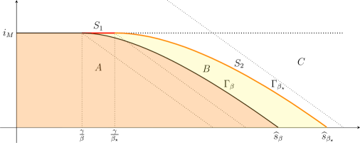
Figure 1. Plot of the regions in Theorem 4.2 for the values $i_{M}=0.4$, $\gamma/\beta=0.2$, $\gamma/\beta_{\star}=0.3$. The orange region represents the maximal forward invariant set $A$ with past in $C$, while the whole colored area represents the set $B$, that is the maximal viable set with past in $C$. The red line $S_{1}$ and the orange curve $S_{2}$ represent the sets in which the control policy in Theorem 4.5 is possibly discontinuous.

Proof.

Let us prove the forward invariance of $\mathcal{A}$ by applying Corollary 2.9 with $\mathcal{K}=\mathcal{A}$. There, the invariance condition is written in terms of the set $D_{\mathcal{A}}$ of feasible directions which, in turn, is characterized in Lemma 2.5 (with $\mathcal{K}_{S}=\mathcal{A}$, $S=C$ and $K=A$) as

$$D_{\mathcal{A}}(\phi)=T_{A}(\phi(0))\;\;\,\forall\phi\in\mathcal{A}.$$

Summarizing, we have to prove that

$$f(\phi,b)\in T_{A}(\phi(0))\quad\forall\,\phi\in\mathcal{A}\ \forall\,b\in[\beta_{\star},\beta],$$ (4.9)

where $f(\phi,b)$ is given in (2.2).

It is enough to consider the case $\phi(0)\in\partial A$, because if $\phi(0)\in\text{Int}(A)$ then $T_{A}(\phi(0))=\mathbb{R}^{n}$ and condition (4.9) is straightforwardly satisfied.

The set $A$ has a piecewise $C^{1}$ boundary and can be written in the form (2.7). Thus, we can use the characterization of $T_{A}(\phi(0))$ given by (2.8). In checking (4.9), by continuity of $f$, we can restrict ourselves to consider only the $\phi(0)$ that belong to the (relative) interior of each piece of $\partial{A}$ and prove that the scalar product of $f(\phi,b)$ with a (outer) normal vector $v\neq 0$ to $A$ in $\phi(0)$ turns out to be non-positive.

Let us then distinguish the following cases corresponding to the relative interior of different pieces of $\partial A$.

1. $i_{\phi}(0)=0$. Since $f(\phi,b)=(-bs_{\phi}(0)i_{\phi}(-h),\;bs_{\phi}(0)i_{\phi}(-h))$ and $v=(0,-1)$ is a normal vector to the halfplane $\{i\geq 0\}$, then we have $\langle v,f\rangle=-bs_{\phi}(0)i_{\phi}(-h)\leq 0,\ \forall b\in[\beta_{\star},\beta].$

2. $s_{\phi}(0)=0$. We have that $f(\phi,b)=\{(0,-\gamma i_{\phi}(0))\}$. Since $v=(-1,0)$ is a normal vector to $A$ at $(s_{\phi}(0),i_{\phi}(0))$ then we have $\langle v,f\rangle=0$.

3. $s_{\phi}(0)<\frac{\gamma}{\beta}$ and $i_{\phi}(0)=i_{M}$. Since $v=(0,1)$, we have

   $$\langle v,f\rangle=bs_{\phi}(0)i_{\phi}(-h)-\gamma i_{\phi}(0)=bs_{\phi}(0)i_{\phi}(-h)-\gamma i_{M}<(\frac{b}{\beta}-1)\gamma i_{M}\leq 0$$

   for every $b\in[\beta_{\star},\beta]$.

4. $s_{\phi}(0)\in(\frac{\gamma}{\beta},\widehat{s}_{\beta})$ and $i_{\phi}(0)=\Gamma_{\beta}(s_{\phi}(0))$. Let us denote, for simplicity, $\phi(0)=(s_{0},i_{0})$ and observe that any normal vector $v=(v_{1},v_{2})\neq 0$ to $A$ at $(s_{0},i_{0})$ satisfies $v_{1}\geq 0$ and $v_{2}\geq 0$. This vector $v$ is, by definition, perpendicular to the tangent vector $(1,\Gamma^{\prime}_{\beta}(s_{0}))$. Since, by (4.6), we have $\Gamma^{\prime}_{\beta}(s_{0})=-1+\frac{\gamma i_{0}}{\beta s_{0}i_{M}}$, then

   $$0=\langle(v_{1},v_{2}),(1,\Gamma^{\prime}_{\beta}(s_{0}))\rangle=v_{1}+\Gamma^{\prime}_{\beta}(s_{0})v_{2}=v_{1}-v_{2}+v_{2}\frac{\gamma i_{0}}{\beta s_{0}i_{M}}$$

   if and only if

   $$0=-(v_{2}-v_{1})\beta s_{0}i_{M}+v_{2}\gamma i_{0},$$

   from which we also deduce that $v_{2}\geq v_{1}$. Then, we have

   $$\langle v,f(\phi,b)\rangle=(v_{2}-v_{1})bs_{0}i_{\phi}(-h)-v_{2}\gamma i_{0}\leq(v_{2}-v_{1})\beta s_{0}i_{M}-v_{2}\gamma i_{0}=0.$$

The proof of forward invariance of $\mathcal{A}$ is thus completed. We now prove the maximality. Consider any set $\widetilde{A}\neq A$ such that $A\subset\widetilde{A}\subseteq C$, and suppose by contradiction that $\widetilde{\mathcal{A}}:=\left\{\phi\in\mathcal{C}\;|\;\phi(0)\in\widetilde{A},\;\phi(s)\in C\;\forall s\in[-h,0]\right\}$ is forward invariant. We can now consider a particular $\phi_{0}\in\widetilde{\mathcal{A}}$ satisfying $\phi_{0}(0)\in\widetilde{A}\setminus A$, i.e.,

$$s_{\phi_{0}}(0)>\frac{\gamma}{\beta},\quad i_{\phi_{0}}(0)>\Gamma_{\beta}(s_{\phi_{0}}(0)),{}$$ (4.10)

and $i_{\phi_{0}}(t)=i_{M}$ for all $t\in[-h,-\varepsilon]$ for a given $\varepsilon\in(0,h)$. Since $\widetilde{\mathcal{A}}$ is supposed to be forward invariant, the solution $(s_{\phi_{0}}(t),i_{\phi_{0}}(t))$ of (1.1) corresponding to the control $b\equiv\beta$ belongs to $\widetilde{A}$ for every $t\in\mathbb{R}_{+}$. Moreover, in the interval $[0,h-\varepsilon]$, it coincides with the solution of the linear system (where $i_{M}$ replaces $i(t-h)$)

$$\begin{cases}s^{\prime}(t)=-\beta i_{M}s(t),\\ i^{\prime}(t)=+\beta i_{M}s(t)-\gamma i(t),\\ \end{cases}$$ (4.11)

with initial condition $(s(0),i(0))=\phi_{0}(0)$. We note that the system (4.11) is the time-inversion of system (4.2), i.e., it is defined by the same vector field with opposite sign. This implies that $i(s)=\Gamma_{\beta}(s)$ represents the graph of a solution of (4.2), as well as (4.11). By uniqueness of solutions of (4.11), inequality (4.10) implies $i_{\phi_{0}}(t)>\Gamma_{\beta}(s_{\phi_{0}}(t))$ for all $t\in[0,h-\varepsilon]$. Thus $(s_{\phi_{0}}(t),i_{\phi_{0}}(t))\notin A$ for all $t\in[0,h-\varepsilon]$, while $(s_{\phi_{0}}(t),i_{\phi_{0}}(t))\in\widetilde{A}$, by forward invariance of $\widetilde{\mathcal{A}}$. We can now iterate the argument, considering a $\phi_{1}\in\widetilde{\mathcal{A}}$ such that $\phi_{1}(0)=(s_{\phi_{0}}(h-\varepsilon),i_{\phi_{0}}(h-\varepsilon))$, and $i_{\phi_{1}}(t)=i_{M}$ for $t\in[-h,-\varepsilon]$. The solution $(s_{\phi_{1}}(t),i_{\phi_{1}}(t))$ to the system (1.1) corresponding to the control $b\equiv\beta$ again coincides in $[0,h-\varepsilon]$, with the solution of (4.11) with initial condition $(s(0),i(0))=\phi_{1}(0)$. Proceeding similarly to define $\phi_{k}\in\widetilde{\mathcal{A}}$, we have that the solutions $(s_{\phi_{k}}(t),i_{\phi_{k}}(t))$ have the property that $i_{\phi_{k}}(t)>\Gamma_{\beta}(s_{\phi_{k}}(t))$ for all $t\in[0,h-\varepsilon]$ and all $k\in\mathbb{N}$. We now join all curves $\phi_{k}$ by considering $\bar{\phi}:\mathbb{R}_{+}\to\mathbb{R}^{2}$ defined by

$$\bar{\phi}(t)=(s_{\bar{\phi}}(t),i_{\bar{\phi}}(t))=\left(s_{\phi_{k}}(t-k(h-\varepsilon)),i_{\phi_{k}}(t-k(h-\varepsilon))\right)\;\;\;\text{if }t\in[k(h-\varepsilon),\,(k+1)(h-\varepsilon)],\;\;k\in\mathbb{N}.$$

By construction we have that $\bar{\phi}(t)\in\widetilde{A}\setminus A$ for all $t\in\mathbb{R}_{+}$, and $\bar{\phi}$ satisfies the Cauchy problem defined by the linear system (4.11) with initial condition $\bar{\phi}(0)=\phi_{0}(0)$. The Cauchy problem for (4.11) with initial condition $(s(0),i(0))=\phi_{0}(0)$ can be explicitly solved. In particular, we have $s_{\bar{\phi}}(t)=s(0)e^{-\beta i_{M}t}$. Since $s(0)>\frac{\gamma}{\beta}$ (see (4.10)), in $T=\frac{1}{\beta i_{M}}\log(\frac{s_{0}\beta}{\gamma})>0$ we have $s_{\bar{\phi}}(T)=\frac{\gamma}{\beta}$. By the uniqueness of solutions of (4.11), we have therefore

$$i_{\bar{\phi}}(T)>\Gamma_{\beta}(s_{\bar{\phi}}(T))=\Gamma_{\beta}(\frac{\gamma}{\beta})=i_{M}.$$

Thus, $\bar{\phi}(T)\notin C\supseteq\widetilde{A}$, leading to a contradiction.

The proof of part (2) of the statement proceeds in a similar way, that is, we prove the viability of $\mathcal{B}$ by applying Corollary 2.9 with $\mathcal{K}=\mathcal{B}$ (see (2.9)) and Lemma 2.5 with $\mathcal{K}_{S}=\mathcal{B}$, $S=C$ and $K=B$. In the current case, we have to prove that

$$\forall\,\phi\in\mathcal{B},\ \exists\,b\in[\beta_{\star},\beta]\,:\,f(\phi,b)\in T_{B}(\phi(0)),$$ (4.12)

where $f(\phi,b)$ is given in (2.2), and it is enough to consider the case $\phi(0)\in\partial B$ (since otherwise $T_{B}(\phi(0))=\mathbb{R}^{n}$).

As before, since the set $B$ has a piecewise $C^{1}$ boundary we can restrict ourselves to consider only the $\phi(0)$ that belong to the (relative) interior of each piece of $\partial{B}$ and prove that the scalar product of $f(\phi,b)$ with a normal vector $v\neq 0$ to $B$ in $\phi(0)$ turns out to be non-positive.

We explicitly develop the non-trivial cases only. In the case $0<s_{\phi}(0)<\frac{\gamma}{\beta_{\star}}$ and $i_{\phi}(0)=i_{M}$, by computing the scalar product of $f(\phi,b)$ with the normal vector $v=(0,1)$, we obtain

$$\langle v,f\rangle=bs_{\phi}(0)i_{\phi}(-h)-\gamma i_{\phi}(0)=bs_{\phi}(0)i_{\phi}(-h)-\gamma i_{M}\leq(b\frac{\gamma}{\beta_{\star}}-\gamma)i_{M},$$

which is non-positive if $b\leq\beta_{\star}$, and thus $f(\phi,\beta_{\star})\in T_{B}(\phi(0))$. Now suppose that $\phi(0)=(s_{0},i_{0})$ is such that $s_{0}\in(\frac{\gamma}{\beta_{\star}},\widehat{s}_{\beta_{\star}})$ and $\Gamma_{\beta_{\star}}(s_{0})=i_{0}$. Again, a normal vector to $B$ at $(s_{0},i_{0})$ is of the form $w=(w_{1},w_{2})\neq 0$, with $w_{1},w_{2}\geq 0$, and, by definition of $\Gamma_{\beta_{\star}}$ it satisfies

$$(w_{2}-w_{1})\beta_{\star}s_{0}i_{M}-w_{2}\gamma i_{0}=0,$$ (4.13)

which also implies $w_{2}\geq w_{1}$. We have

$$\langle w,f(\phi,\beta_{\star})\rangle=(w_{2}-w_{1})\beta_{\star}s_{0}i_{\phi}(-h)-w_{2}\gamma i_{0}\leq(w_{2}-w_{1})\beta_{\star}s_{0}i_{M}-w_{2}\gamma i_{0}=0,$$

and (4.12) is satisfied. This proves that $\mathcal{B}$ is viable. The maximality follows by an argument analogous to the one used in proving (1). ∎

Besides the state equation (1.1) and the state constraint (1.3), we consider now a cost functional of the form

$$J(u):=\int_{0}^{\infty}G(u(t))\;dt,$$ (4.14)

where $u(t):=\beta-b(t)$ and $G:\mathbb{R}_{+}\to\mathbb{R}_{+}$ is a convex and strictly increasing function, satisfying $G(0)=0$.

Problem 4.3 (Optimal Control Problem $\mathcal{P}_{\phi}$.).

Given the initial data $\phi\in\mathcal{C}$, minimize over all admissible controls $u\in\mathcal{U}$

• the cost functional (4.14),

• under the ICU constraint (1.3) on the trajectory of  (1.1).

In the sequel we refer to this formulation as problem $\mathcal{P}_{\phi}$.

We first prove that a solution to the optimal control problem $\mathcal{P}_{\phi}$ exists, for initial conditions in $\mathcal{C}$.

Theorem 4.4.

For any initial condition $\phi\in\mathcal{C}$, the optimal control problem $\mathcal{P}_{\phi}$ admits a solution.

Proof.

Let us denote for simplicity $I=(0,+\infty)$. To prove the existence of an optimal solution we observe that it is equivalent to prove the existence of a minimizer of the functional $J^{\infty}:L^{\infty}(I;[0,\beta-\beta_{\star}])\times W^{1,\infty}(I;\mathbb{R}^{2})\to[0,+\infty]$ defined by

$$J^{\infty}(u,s,i):=J(u)+\chi_{\Lambda}(u,s,i)+\chi_{i\leq i_{M}}(i),$$ (4.15)

where $\Lambda$ is the set of admissible pairs, that is all control-state vectors $(u,s,i)$ that satisfy the initial value problem for the state equation (1.1) with initial condition $\phi\in\mathcal{C}$, while $\chi_{\Lambda}$ denotes the indicator function of $\Lambda$ that takes the value $0$ on $\Lambda$ and $+\infty$ otherwise; similarly, the function $\chi_{i\leq i_{M}}(i)$ is $0$ if $i(t)\leq i_{M}$ for every $t\in I$, and $+\infty$ otherwise.

On the domain of $J^{\infty}$ we consider the topology given by the product of the weak* topologies of the spaces $L^{\infty}$ and $W^{1,\infty}$, and aim to prove sequential lower semicontinuity and coercivity of the functional $J^{\infty}$ with respect to this topology. By the Direct Method of the Calculus of Variations (see, for instance, Buttazzo [10, Sec. 1.2]), these properties imply the existence of a solution to the minimum problem. They are direct consequences of the fact that the space of controls is weakly* compact, that the assumptions on the integrand imply that the cost functional $J$ is weakly* lower semicontinuous (see, for instance, [16, Theorem 5.1]) and the fact that the sets $\Lambda$ and $\{i\leq i_{M}\}$ are closed with respect to the weak* convergence. The claimed closedness of such sets follows by the application of Rellich compactness theorem, which ensures that weakly* converging sequences in $W^{1,\infty}(I)$ are, up to subsequences, uniformly converging on every bounded subinterval of $I$ (see for instance [9, Theorem 8.8 and Remark 10]). To prove it in details, let us consider a sequence $(u_{n},s_{n},i_{n})\in\Lambda$ weakly* converging in $L^{\infty}(I)\times W^{1,\infty}(I,\mathbb{R}^{2})$ to $(u,s,i)$ and satisfying $i_{n}\leq i_{M}$ for every $n\in\mathbb{N}$. Then, we easily get that $i_{n}(\cdot-h)=i_{\phi}1_{[0,h]}+i_{n}1_{(h,+\infty)}$ weakly* converges to $i(\cdot-h)=i_{\phi}1_{[0,h]}+i1_{(h,+\infty)}$ in $L^{\infty}(I)$. Then we can pass to the limit in the state equations and, by uniqueness of the limit, we obtain that $(u,s,i)\in\Lambda$. Moreover, $i\leq i_{M}$ by the local uniform convergence. ∎

The performed viability analysis provides a route for designing a state-dependent control policy in order to minimize/bound the cost (4.14) and to fulfill the state constraint (1.3). Indeed, in Theorem 4.2 we have proven that, for any initial condition $\phi\in\mathcal{B}$, there exists at least a control action for which the corresponding solution satisfies $S(t)x_{\phi}\in\mathcal{B}$ for all $t\in\mathbb{R}_{+}$. Rephrasing, we have proven that the so-called regulation map (see [3, Definition 6.1.2])

$$U_{\mathcal{B}}(\phi):=\{b\in[\beta_{\star},\beta]\;|\;f(\phi,b)\in D_{\mathcal{B}}(\phi)\},$$

in non-empty for every $\phi\in\mathcal{B}$.

In what follows, we explicitly select a (in general, sub-optimal) control $b(\phi)\in U_{\mathcal{B}}(\phi)$ by minimizing the function $G$ in (4.14), i.e., we consider

$$b(\phi)=\arg\min_{b\in U_{\mathcal{B}}(\phi)}G(\beta-b)=\max\{b\in U_{\mathcal{B}}(\phi)\}.$$

This idea is formalized in the subsequent statement.

Theorem 4.5 (greedy control policy).

Let $\Gamma_{\beta_{\star}}:[\frac{\gamma}{\beta_{\star}},\widehat{s}_{\beta_{\star}}]\to[0,i_{M}]$ be the curve defined in (4.7) and $B\subset C$ be the set defined in (4.8). Let us introduce the sets

$$S_{1} :=\text{\emph{co}}\big{\{}(\frac{\gamma}{\beta},i_{M}),\,(\frac{\gamma}{\beta_{\star}},i_{M})\big{\}}\subset\partial B,$$

$$S_{2} :=\big{\{}(s,i)\in T\ |\ s\in[\frac{\gamma}{\beta_{\star}},\widehat{s}_{\beta_{\star}}]\text{ and }i=\Gamma_{\beta_{\star}}(s)\big{\}}\subset\partial B,$$

and consider the state-feedback control policy $\widetilde{b}:\mathcal{B}\to[\beta_{\star},\beta]$ given by

$$\widetilde{b}(\phi)=\begin{cases}\beta,\;\;\;&\text{if }\phi(0)\in B\setminus(S_{1}\cup S_{2}),\\ \min\big{\{}\beta,\frac{\gamma i_{M}}{s_{\phi}(0)i_{\phi}(-h)}\big{\}},\;\;\;&\text{if }\phi(0)\in S_{1},\\ \min\big{\{}\beta,\;\beta_{\star}\frac{i_{M}}{i_{\phi}(-h)}\big{\}},\;\;\;&\text{if }\phi(0)\in S_{2},\end{cases}$$ (4.16)

with the convention $1/0=+\infty$. Given the function $\widetilde{F}:\mathcal{B}\to\mathbb{R}^{2}$ defined by $\widetilde{F}(\phi)=f(\phi,\widetilde{b}(\phi))$ (with $f$ defined in (2.1)), there exists a solution $x_{\phi}:[-h,+\infty)\to\mathbb{R}^{2}$ to

$$\begin{cases}x^{\prime}(t)=\widetilde{F}(S(t)x),\\ S(0)x=\phi\in\mathcal{B},\end{cases}$$ (4.17)

where the operator $S(t)$ has been introduced in (2.3).

Given any $\phi\in\mathcal{B}$, we have that

1. $x_{\phi}(t)\in B$ for all $t\in\mathbb{R}_{+}$;

2. defining $\widetilde{b}_{\phi}:\mathbb{R}_{+}\to[\beta_{\star},\beta]$ by

   $$\widetilde{b}_{\phi}(t):=\widetilde{b}(S(t)x_{\phi}),$$ (4.18)

   with $\widetilde{b}$ defined as in (4.16), it holds that

   1. $x_{\phi}$ is the unique solution to the Cauchy problem (1.1)-(1.2) with $b=\widetilde{b}_{\phi}$;

   2. $\widetilde{b}_{\phi}$ is eventually constant equal to $\beta$;

   3. the corresponding cost (4.14) is finite.

Moreover, if $\phi\in\mathcal{B}\cap\mathcal{T}_{0}$ (i.e., avoiding the trivial case of $i_{\phi}$ identically zero in $[-h,0]$), we also have

1. there exists a $T=T(\phi)\geq 0$ such that $x_{\phi}(t)\in R$ (see (4.8)) for all $t\geq T$.

Remark 4.6.

1. The control $\widetilde{b}(\phi)$ is well-defined for $\phi$ such that $\phi(0)\in S_{1}\cap S_{2}$. Indeed, if $\phi(0)\in S_{1}\cap S_{2}=\{(\frac{\gamma}{\beta_{\star}},i_{M})\}$ we have $\frac{\gamma i_{M}}{s_{\phi}(0)i_{\phi}(-h)}=\beta_{\star}\frac{i_{M}}{i_{\phi}(-h)}$.

2. The case in which $\widetilde{b}(\phi)=\beta_{\star}$ only occurs when $\phi(0)\in S_{2}$ and $i_{\phi}(-h)=i_{M}$. Hence, the case in which $\widetilde{b}_{\phi}(t)=\beta_{\star}$ for a.e. $t$ in an interval $J$ only occurs when $(s_{\phi}(t),i_{\phi}(t))\in S_{2}$ and $i_{\phi}(t-h)=i_{M}$ for all $t\in J$. This scenario may happen only in the time interval $[0,h]$ and for a suitable initial condition. Then, in general, one cannot expect that a constant control regime $\widetilde{b}_{\phi}=\beta_{\star}$ occurs, except than in some very particular cases.

Proof.

First of all we observe that the feedback control policy $\widetilde{b}$, defined in (4.16), takes values in $[\beta_{\star},\beta]$. This is not trivial only in the case in which $\phi(0)\in S_{1}$. In this case we have $s_{\phi}(0)\leq\frac{\gamma}{\beta_{\star}}$ and, recalling also that $\phi\in\mathcal{B}$ implies $i_{\phi}(-h)\leq i_{M}$, we have

$$\frac{\gamma i_{M}}{s_{\phi}(0)i_{\phi}(-h)}\geq\beta_{\star},$$

thus proving that $\widetilde{b}(\phi)\in[\beta_{\star},\beta]$, as claimed.

As a preliminary step to the proof of existence of a solution to the Cauchy problem (4.17), we prove that

$$\widetilde{F}(\phi)\in\mathcal{D}_{\mathcal{B}}(\phi)\;\,\forall\,\phi\in\mathcal{B}.$$ (4.19)

To this aim we note that, by Lemma 2.5, we have $\mathcal{D}_{\mathcal{B}}(\phi)=T_{\mathcal{B}}(\phi(0))$ for every $\phi\in\mathcal{B}$. Since $\phi(0)\in\text{Int}(B)$ implies $\mathcal{D}_{\mathcal{B}}(\phi)=T_{B}(\phi(0))=\mathbb{R}^{n}$, it suffices to consider the case $\phi(0)\in\partial B$. Given $\phi\in\mathcal{B}$, it is convenient to distinguish the following four cases.

1. $\phi(0)\in\partial B\setminus(S_{1}\cup S_{2})$. If $\phi(0)$ lies on the horizontal axis, the statement is trivial. In the case $\phi(0)\in A\cap\partial B$, since $\mathcal{A}$ is forward invariant (see Theorem 4.2), Corollary 2.9 implies that $\widetilde{F}(\phi)=f(\phi,\beta)\in D_{\mathcal{A}}(\phi)$ which, in turn, is contained in $D_{\mathcal{B}}(\phi)$. Therefore, (4.19) is proved in this case.

2. $\phi(0)\in S_{1}\setminus S_{2}$. In this case we have $s_{\phi}(0)\in[\frac{\gamma}{\beta},\frac{\gamma}{\beta_{\star}})$ and $i_{\phi}(0)=i_{M}$. At the point $\phi(0)$, we compute the scalar product of the vector field with the (unique, modulo positive scalar multiplication) normal vector $v=(0,1)$ to $B$ at $\phi(0)$, so obtaining

   $$\langle v,f(\phi,\widetilde{b}(\phi))\rangle=\widetilde{b}(\phi)s_{\phi}(0)i_{\phi}(-h)-\gamma i_{M}=\widetilde{b}(\phi)s_{\phi}(0)i_{\phi}(-h)-\gamma i_{M}.$$ (4.20)

   Let us suppose, first, that $\widetilde{b}(\phi)=\min\left\{\beta,\frac{\gamma i_{M}}{s_{\phi}(0)i_{\phi}(-h)}\right\}=\frac{\gamma i_{M}}{s_{\phi}(0)i_{\phi}(-h)}$. Then we have

   $$\widetilde{b}(\phi)s_{\phi}(0)i_{\phi}(-h)-\gamma i_{M}=\frac{\gamma i_{M}}{s_{\phi}(0)i_{\phi}(-h)}s_{\phi}(0)i_{\phi}(-h)-\gamma i_{M}=0,$$

   proving that the vector field is tangent to the line $\{(s,i)\in\mathbb{R}^{2}\;|\;i=i_{M}\}$. If, on the contrary, we have $\widetilde{b}(\phi)=\beta$, this implies that $\beta\leq\frac{\gamma i_{M}}{s_{\phi}(0)i_{\phi}(-h)}$ and thus

   $$\widetilde{b}(\phi)s_{\phi}(0)i_{\phi}(-h)-\gamma i_{M}=\beta s_{\phi}(0)i_{\phi}(-h)-\gamma i_{M}\leq 0,$$

   and the equality holds only if $\beta=\frac{\gamma i_{M}}{s_{\phi}(0)i_{\phi}(-h)}$. Then, we have proven that $f(\phi,\widetilde{b}(\phi))\in T_{B}(\phi(0))=\mathcal{D}_{\mathcal{B}}(\phi)$, that is (4.19).

3. $\phi(0)\in S_{2}\setminus S_{1}$. In this case $s_{\phi}(0)\in(\frac{\gamma}{\beta_{\star}},\widehat{s}_{\beta_{\star}}]$ and $i_{\phi}(0)=\Gamma_{\beta_{\star}}(s_{\phi}(0))$. At the point $(s_{\phi}(0),i_{\phi}(0))$ the unique (modulo positive scalar multiplication) normal to the set $B$ is a vector $v=(v_{1},v_{2})$ for some $v_{1},v_{2}\geq 0$ such that

   $$(v_{2}-v_{1})\beta_{\star}s_{\phi}(0)i_{M}-v_{2}\gamma i_{\phi}(0)=0,$$

   by definition of $\Gamma_{\beta_{\star}}$. Suppose first that $\widetilde{b}(\phi)=\beta_{\star}\frac{i_{M}}{i_{\phi}(-h)}$, i.e., $\beta\geq\beta_{\star}\frac{i_{M}}{i_{\phi}(-h)}$. By the previous equality, we have

   $$\langle v,f(\phi,\widetilde{b}(\phi))\rangle=(v_{2}-v_{1})\beta_{\star}\frac{i_{M}}{i_{\phi}(-h)}s_{\phi}(0)i_{\phi}(-h)-v_{2}\gamma i_{\phi}(0)=0.$$

   Suppose now that $\widetilde{b}(\phi)=\beta$, i.e., $\beta\leq\beta_{\star}\frac{i_{M}}{i_{\phi}(-h)}$. Then

   $$\langle v,f(\phi,\widetilde{b}(\phi))\rangle=(v_{2}-v_{1})\beta s_{\phi}(0)i_{\phi}(-h)-v_{2}\gamma i_{\phi}(0)\leq(v_{2}-v_{1})\beta_{\star}s_{\phi}(0)i_{M}-v_{2}\gamma i_{\phi}(0)=0,$$

   and, again, the equality holds only if and only if $\beta=\beta_{\star}\frac{i_{M}}{i_{\phi}(-h)}$. This proves that $f(\phi,\widetilde{b}(\phi))\in T_{B}(\phi(0)=\mathcal{D}_{\mathcal{B}}(\phi)$, that is (4.19) also in the current case.

4. $\phi(0)\in S_{1}\cap S_{2}$. In this case, $\phi(0)=(\frac{\gamma}{\beta_{\star}},i_{M})$ and the claim follows by items (b) and (c), through a continuity argument.

We have thus proven (4.19). Under this condition, the existence of solutions $x_{\phi}$ to (4.17) is proved in Lemma A.1 in Appendix, together with the property $S(t)x_{\phi}\in\mathcal{B}$, for all $t\in\mathbb{R}_{+}$, which implies $S(t)x_{\phi}(0)=x_{\phi}(t)\in B$, for all $t\in\mathbb{R}_{+}$. Then, part (1) of the statement is proved.

To prove (2)(a), it is enough to observe that

$$\widetilde{F}(S(t)x_{\phi})=f(S(t)x_{\phi},\widetilde{b}_{\phi}(t))=(-\widetilde{b}_{\phi}(t)s_{\phi}(t)i_{\phi}(t-h)\,,\,\widetilde{b}_{\phi}(t)s_{\phi}(t)i_{\phi}(t-h)-\gamma i_{\phi}(t)),$$

which means that the solution $x_{\phi}$ to (4.17) is also a solution to (1.1)-(1.2) with $b=\widetilde{b}_{\phi}$, and such Cauchy problem has a unique solution by Lemma 2.1. Of course, this implies (a posteriori) that also (4.17) has a unique solution.

Let us now prove (2)(b). In Lemma 3.1 we have proven that $\lim_{t\to+\infty}i_{\phi}(t)=0$ and $s_{\phi,\infty}=\lim_{t\to+\infty}s_{\phi}(t)\in[0,\frac{\gamma}{\beta_{\star}})$. Then, there exists a $T_{1}(\phi)\geq 0$ such that $x_{\phi}(t)\notin S_{1}\cup S_{2}$ for all $t\geq T_{1}(\phi)$. By (4.16) and (4.18), this implies that $b_{\phi}(t)=b(S(t)x_{\phi})=\beta$ for all $t\geq T_{1}(\phi)$, since $S(t)x_{\phi}(0)=x_{\phi}(t)\notin S_{1}\cup S_{2}$. This proves (2)(b).

(2)(c) holds since

$$\int_{0}^{+\infty}G(\beta-\widetilde{b}_{\phi}(t))\,dt=\int_{0}^{T_{1}(\phi)}G(\beta-\widetilde{b}_{\phi}(t))\,dt\leq\int_{0}^{T_{1}(\phi)}G(\beta-\beta_{\star})\,dt=T_{1}(\phi)G(\beta-\beta_{\star}).$$

To prove part (3), suppose $\phi\in\mathcal{B}\cap\mathcal{T}_{0}$. Since we have proven that $b_{\phi}$ is eventually equal to $\beta$, by part (2) of Lemma 3.1 we have that $s_{\phi,\infty}\in[0,\frac{\gamma}{\beta})$, which in turns implies that there exists a $T=T(\phi)\geq 0$ such that $s_{\phi}(t)\leq\frac{\gamma}{\beta}$ (and thus $x_{\phi}(t)\in R$) for all $t\geq T$, and the proposition is completely proved. ∎

A first direct consequence of the existence of the “greedy” feedback control policy defined in (4.16) is stated below.

Corollary 4.7.

For any prescribed initial condition $\phi\in\mathcal{B}$, the optimal control problem $\mathcal{P}_{\phi}$ admits a solution with a finite cost.

Proof.

The proof directly follows by Theorem 4.4 and assertion (3) of Theorem 4.5. ∎

Remark 4.8.

We note that the invariance/viability regions in Theorem 4.2 are independent of $h$. In particular, they do not converge, as $h\to 0$, to the regions obtained in the delay-free case (see [15, 4, 16]), recalled also in the subsequent Theorem 4.13. In the next subsection we strenghten Assumption 4.1 by bounding the velocity of the past evolution of the epidemic. This allows us to obtain a viability analysis and a control policy which do depend on the parameter $h>0$, and that converge, in a sense that will be clarified, to the solutions provided for the delay-free case.

4.2. Lipschitz continuous initial conditions

In the previous subsection, we supposed to have limited information on the past evolution of the epidemic, only considering Assumption 4.1. We hereafter assume that, in the past $h$ time units, the epidemic dynamic not only was under the warning level (i.e. $i_{\phi}(t)\leq i_{M}$ for all $t\in[-h,0]$), but also was evolving with a limited “speed”, compatible with the epidemic model. More formally we assume the following.

Assumption 4.9.

Given a threshold $0<i_{M}\leq 1$ consider any $L\in\mathbb{R}$ such that

$$L\geq i_{M}\max\{\beta,\gamma\}>0.$$ (4.21)

We assume that the initial condition $\phi\in\mathcal{C}$ of (1.1) satisfies

$$\phi(t)\in C\;\;\;\forall\;t\in[-h,0],$$

with $C=\{(s,i)\in T\;|\;i\leq i_{M}\}$, and

$$\phi\in\mathcal{C}_{L,|\cdot|_{\max}}=\{\varphi\in\mathcal{C}\;|\;|\varphi(t_{1})-\varphi(t_{2})|_{\max}\leq L|t_{1}-t_{2}|\;\;\forall t_{1},t_{2}\in[-h,0]\},$$

where $|x|_{\max}:=\max\{|x_{1}|,|x_{2}|\}$, for any $x=(x_{1},x_{2})\in\mathbb{R}^{2}$.

Remark 4.10.

The choice of the infinity/max norm is motivated by the fact that the dynamics in (1.1) are only affected by the delayed value of the $i$-component ($i(-h)$), while the delayed $s$-component ($s(-h)$) does not play any role. The $\max$ norm, which, intuitively, is only affected by the “worst case” of any component (considered separately), is thus a natural choice. Nevertheless, the subsequent analysis can be adapted to the choice of any other norm in $\mathbb{R}^{2}$.

Remark 4.11.

The lower bound (4.21) on the Lipschitz constant $L>0$ is motivated by noting that, for any $x=(s,i)\in C$ such that $i\leq i_{M}$ we have

$$|-\beta si|\leq\beta i_{M}\,\;\text{ and }\,\;|\beta si-\gamma i|\leq i_{M}\max\{\beta,\gamma\}.$$

Thus,

$$|f(\phi,b)|_{\max}\leq L\;\;\;\forall\,\phi\in\mathcal{C},\;\forall\,b\in U,$$ (4.22)

and, hence, $L\geq i_{M}\max\{\beta,\gamma\}$ represents a uniform upper bound to the speed modulus of the solution to (1.1) with initial condition $\phi\in\mathcal{C}$ such that $\phi(s)\in C$, for all $s\in[-h,0]$. Intuitively, in Assumption 4.9, we are supposing that the epidemic, in the past uncontrolled interval of time $[-h,0]$, has evolved at a bounded speed, and this bound is assumed to be not smaller than the one holding forward in time, according with the model.

In order to retrace the analysis performed in Subsection 4.1, we need to introduce auxiliary (non-delayed) systems that mimic the “worst-case” behaviour of the delay system  (1.1). Since the considered initial conditions are supposed to satisfy Assumption 4.9, we first define a scalar function that models the maximal gap between $i(0)$ and $i(-h)$. Namely, for any $L,h>0$, we consider the Lipschitz continuous function $\psi_{L,h}:\mathbb{R}\to\mathbb{R}$ (see Figure 2) defined by

$$\psi_{L,h}(i):=\begin{cases}-i_{M},\;\;\;&\text{if }i\leq-i_{M}-Lh,\\ i+Lh,\;\;\;&\text{if }-i_{M}-Lh<i\leq i_{M}-Lh,\\ i_{M},\;\;\;&\text{if }i_{M}-Lh<i.\end{cases}$$ (4.23)

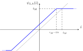
Figure 2. The truncating function $\psi_{L,h}$ defined in (4.23).

Let us now consider the non-linear differential equation

$$\begin{cases}s^{\prime}(t)=\;\;\beta s(t)\psi_{L,h}(i(t)),\\ i^{\prime}(t)=-\beta s(t)\psi_{L,h}(i(t))+\gamma i(t).\end{cases}$$ (4.24)

The right-hand side in (4.24) is locally Lipschitz, and since $|\psi_{L,h}(i)|\leq i_{M}$ for all $i\in\mathbb{R}$, we also have that

$$|(\beta s\psi_{L,h}(i)\,,\,-\beta s\psi_{L,h}(i)+\gamma i)|_{\max}\leq A|(s,i)|_{\max},\;\;\forall(s,i)\in\mathbb{R}^{2},$$ (4.25)

for a suitable $A>0$. This implies that, for any prescribed initial condition, the solution to (4.24) is unique and globally defined, see [37, Theorem 2.17]. We thus denote by $\Psi_{\beta,L,h}=(\bar{s}_{\beta,L,h},\,\bar{\imath}_{\beta,L,h}):\mathbb{R}_{+}\to\mathbb{R}^{2}$ the solution to (4.24) corresponding to the initial condition $(s(0),i(0))=(\frac{\gamma}{\beta},i_{M})$. We define

$$T_{\beta,L,h}:=\sup\{\bar{t}\geq 0\;|\;\bar{\imath}_{\beta,L,h}(t)>0\;\,\forall\,t\in[0,\bar{t})\}.$$

Let us denote $\widehat{s}_{\beta,L,h}:=\lim_{t\to T_{\beta,L,h}^{-}}\bar{s}_{\beta,L,h}(t)$. Since the solutions to (4.24) satisfy $s(t)=s_{0}\,e^{\beta\int_{0}^{t}\psi_{L,h}(i(\tau))\,d\tau}$ and $\psi_{L,h}(i)>0$ for any $i\in\mathbb{R}_{+}$, we have that $\bar{s}_{\beta,L,h}$ is strictly positive and strictly increasing in $[0,T_{\beta,L,h})$.

Thus, we can define $\Gamma_{\beta,L,h}:[\frac{\gamma}{\beta},\widehat{s}_{\beta,L,h})\to\mathbb{R}_{+}$ as the function representing the curve $\Psi_{\beta,L,h}$ in $[0,T_{\beta,L,h})$ as a graph $i(s)=\Gamma_{\beta,L,h}(s)$. In Lemma A.2 in Appendix we show that $\Gamma_{\beta,L,h}$ is strictly decreasing and concave in $[\frac{\gamma}{\beta},\widehat{s}_{\beta,L,h})$. Since $\lim_{s\to\widehat{s}_{\beta,L,h}^{\,-}}\Gamma_{\beta,L,h}(s)\geq 0$, we have that $\widehat{s}_{\beta,L,h}$ is finite. In turn, this implies that $T_{\beta,L,h}<+\infty$. Indeed, suppose by contradiction that $T_{\beta,L,h}=+\infty$; then $\bar{s}_{\beta,L,h}^{\prime}(t)=\beta\bar{s}_{\beta,L,h}(t)\psi_{L,h}(\bar{\imath}_{\beta,L,h}(t))\geq\gamma Lh$ for all $t\in(0,T_{\beta,L,h})=(0,+\infty)$, in contradiction with $\widehat{s}_{\beta,L,h}=\lim_{t\to T_{\beta,L,h}^{-}}\bar{s}_{\beta,L,h}(t)<+\infty$. Moreover, recalling that $\bar{s}_{\beta,L,h}(t)$ is continuous and strictly increasing, $T_{\beta,L,h}<+\infty$ implies that

$$\lim_{s\to\widehat{s}_{\beta,L,h}^{-}}\Gamma_{\beta,L,h}(s)=\lim_{t\to T_{\beta,L,h}^{-}}\Gamma_{\beta,L,h}(\bar{s}_{\beta,L,h}(t))=\lim_{t\to T_{\beta,L,h}^{-}}\bar{\imath}_{\beta,L,h}(t)=0,$$

where the last equality follows by definition of $T_{\beta,L,h}$. We can thus extend $\Gamma_{\beta,L,h}$ on the closed interval $[\frac{\gamma}{\beta},\widehat{s}_{\beta,L,h}]$ by setting $\Gamma_{\beta,L,h}(\widehat{s}_{\beta,L,h})=0$. See Figure 3 for a graphical representation of such curve.

Similarly, denote by $\Psi_{\beta_{\star},L,h}=(\bar{s}_{\beta_{\star},L,h},\,\bar{\imath}_{\beta_{\star},L,h}):\mathbb{R}_{+}\to\mathbb{R}^{2}$ the solution to the differential equation

$$\begin{cases}s^{\prime}(t)=\;\;\beta_{\star}s(t)\psi_{L,h}(i(t))\\ i^{\prime}(t)=-\beta_{\star}s(t)\psi_{L,h}(i(t))+\gamma i(t)\end{cases}$$ (4.26)

with initial condition $(s(0),i(0))=(\frac{\gamma}{\beta_{\star}},i_{M})$. We consider $T_{\beta_{\star},L,h}:=\sup\{\bar{t}\geq 0\;|\;\bar{\imath}_{\beta^{\star},L,h}(t)>0\;\,\forall\,t\in[0,\bar{t})\}$, define $\widehat{s}_{\beta_{\star},L,h}:=\lim_{t\to T_{\beta_{\star},L,h}^{-}}\bar{s}_{\beta_{\star},L,h}(t)$, and represent the curve $\Psi_{\beta_{\star},L,h}:[0,T_{\beta_{\star},L,h})\to\mathbb{R}^{2}$ as a graph $i(s)=\Gamma_{\beta_{\star},L,h}(s)$, with $\Gamma_{\beta_{\star},L,h}:[\frac{\gamma}{\beta_{\star}},\widehat{s}_{\beta_{\star},L,h})\to\mathbb{R}_{+}$, see Figure 3. In Lemma A.2, it is proved that $\Gamma_{\beta_{\star},L,h}$ is concave and strictly decreasing, also implying that $\widehat{s}_{\beta_{\star},L,h}$ is finite. Arguing as before, we can thus extend $\Gamma_{\beta_{\star},L,h}$ by continuity on $[\frac{\gamma}{\beta_{\star}},\widehat{s}_{\beta_{\star},L,h}]$ by setting $\Gamma_{\beta_{\star},L,h}(\widehat{s}_{\beta_{\star},L,h})=0$.

We can now provide the viability result.

Theorem 4.12.

Consider the sets $R,R_{\star}\subset C$ defined in (4.8), and define the sets $A_{L,h},B_{L,h}\subset C$ by

$$A_{L,h} :=R\cup\Big{\{}(s,i)\in T\;|\;s\in[\frac{\gamma}{\beta},\widehat{s}_{\beta,L,h}],\;\,i\leq\Gamma_{\beta,L,h}(s)\Big{\}},$$ (4.27)

$$B_{L,h} :=R_{\star}\cup\Big{\{}(s,i)\in T\;|\;s\in[\frac{\gamma}{\beta_{\star}},\widehat{s}_{\beta_{\star},L,h}],\;\,i\leq\Gamma_{\beta_{\star},L,h}(s)\Big{\}}.$$

The following propositions hold.

1. $A_{L,h}$ is the maximal forward invariant set with $\mathcal{C}_{L,|\cdot|_{\max}}$-past in $C$.

2. $B_{L,h}$ is the maximal viable set with $\mathcal{C}_{L,|\cdot|_{\max}}$-past in $C$.

Proof.

The idea behind the proof is essentially the same of the proof of Theorem 4.2, and it relies on Lemma 2.5 and Corollary 2.9. We start by proving that $\mathcal{A}_{L,h}=\left\{\phi\in\mathcal{C}_{L,|\cdot|_{\max}}\;|\;\phi(0)\in A_{L,h},\;\;\phi(s)\in C\;\,\forall\,s\in[-h,0]\right\}$ is forward invariant. As always, it is enough to consider $\phi\in\mathcal{A}_{L,h}$ such that $\phi(0)\in\partial A_{L,h}$ and prove that $F_{U}(\phi)\subseteq T_{A_{L,h}}(\phi(0))\cap B_{|\cdot|_{\max}}(0,L)$. By (4.22), it sufficies to prove that

$$F_{U}(\phi)\subseteq T_{A_{L,h}}(\phi(0)).$$ (4.28)

Let us consider two cases.

1. Given the set $D=\{(s,i)\in T\;|\;s\leq\frac{\gamma}{\beta}\}$, we note that $A\cap D=A_{L,h}\cap D$. Hence, in $D$ the analysis performed for $A$ in Theorem 4.2 applies also to $A_{L,h}$. Therefore, the inclusion (4.28) holds true in the case $\phi(0)\in\partial A_{L,h}\cap D$.

2. In the remaining case, in which $\phi(0)=(s_{0},i_{0})$ with $s_{0}\in(\frac{\gamma}{\beta},\widehat{s}_{\beta,L,h}]$ and $i_{0}=\Gamma_{\beta,L,h}(s_{0})$, we denote the unique normal vector (up to positive scalar multiplication) to $A_{L,h}$ at $(s_{0},i_{0})$ by $v=(v_{1},v_{2})\in\mathbb{R}^{2}\setminus\{0\}$. It is, by definition, perpendicular to the tangent vector $(1,\Gamma^{\prime}_{\beta,L,h}(s_{0}))$. Since $\Gamma^{\prime}_{\beta,L,h}(s_{0})<0$ (by Lemma A.2), we have that $v_{1}\geq 0,v_{2}\geq 0$, and (by normality)

   $$0=v_{1}\beta s_{0}\psi_{L,h}(i_{0})-v_{2}\beta s_{0}\psi_{L,h}(i_{0})+v_{2}\gamma i_{0}=-(v_{2}-v_{1})\beta s_{0}\psi_{L,h}(i_{0})+v_{2}\gamma i_{0},$$ (4.29)

   also proving that $v_{2}\geq v_{1}$. We note that, by Assumption 4.9, we have $i_{\phi}(-h)\leq\min\{i_{M},\,i_{0}+Lh\}=\psi_{L,h}(i_{0})$. Considering any $b\in[\beta_{\star},\beta]$ and using (4.29), we obtain

   $$\langle v,f(\phi,b)\rangle=(v_{2}-v_{1})bs_{0}i_{\phi}(-h)-v_{2}\gamma i_{0}\leq(v_{2}-v_{1})\beta s_{0}\psi_{L,h}(i_{0})-v_{2}\gamma i_{0}=0,$$

   which proves (4.28) also in this case.

This concludes the proof of forward invariance of $\mathcal{A}_{L,h}$. The proofs of maximality of $A_{L,h}$ and assertion (2) follow by arguments similar to the ones provided in the proof of Theorem 4.2, and are left to the reader. ∎

Differently from the viability analysis performed in Theorem 4.2, the regions defined in Theorem 4.12 do depend on the delay parameter $h>0$. We will show that they converge, in a sense we are going to clarify, to the invariance/viability regions for the delay-free case, as $h\to 0$. To this aim, let us summarize here the main viability and invariance results obtained in [4, Section 2] for the delay-free system of ordinary differential equations

$$\begin{cases}s^{\prime}(t)=-b(t)s(t)i(t),\\ i^{\prime}(t)=b(t)s(t)i(t)-\gamma i(t).\end{cases}$$ (4.30)

Theorem 4.13 (Theorem 2.3, [4]).

The following propositions hold true for the delay-free system (4.30).

1. The maximal forward invariant set contained in $C$ (the all-control zone $\mathcal{A}$ in [4]) , is given by

   $$A_{0}:=\{x=(s,i)\in C\;|\;s\leq\Gamma_{\beta,0}(s)\},$$

   where

   $$\Gamma_{\beta,0}(s)=\begin{cases}i_{M},\;\;\;\;&\text{if }0\leq s\leq\frac{\gamma}{\beta},\\ \frac{\gamma}{\beta}+i_{M}-s+\frac{\gamma}{\beta}\log(\frac{\beta}{\gamma}s),\;\;\;&\text{if }s\geq\frac{\gamma}{\beta}.\end{cases}$$ (4.31)

2. The maximal viable set contained in $C$ (the feasible set $\mathcal{B}$ in [4]), is given by

   $$B_{0}:=\{x=(s,i)\in C\;|\;s\leq\Gamma_{\beta_{\star},0}(s)\},$$

   where

   $$\Gamma_{\beta_{\star},0}(s)=\begin{cases}i_{M},\;\;\;\;&\text{if }0\leq s\leq\frac{\gamma}{\beta_{\star}},\\ \frac{\gamma}{\beta_{\star}}+i_{M}-s+\frac{\gamma}{\beta_{\star}}\log(\frac{\beta_{\star}}{\gamma}s),\;\;\;&\text{if }s\geq\frac{\gamma}{\beta_{\star}}.\end{cases}$$

Remark 4.14.

We have chosen to denote the maximal sets by $A_{0}$ and $B_{0}$ instead than $\mathcal{A}$ and $\mathcal{B}$ as in [4] to stress the fact that these sets corresponds to the delay $h=0$.

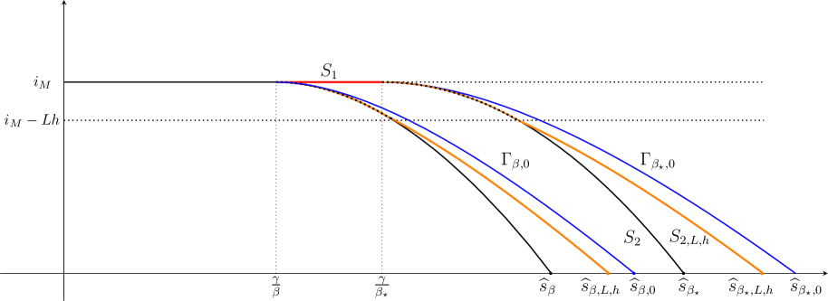
Figure 3. The figure shows qualitatite graphs curves introduced in Theorem 4.12, Lemma 4.17 and Proposition 4.18. In orange we plot the graphs of the functions $\Gamma_{\beta,L,h}$ and $\Gamma_{\beta_{\star},L,h}$. In black the curves $\Gamma_{\beta}$ and $\Gamma_{\beta_{\star}}$ corresponding to the case studied in Subsection 4.1, while in blue the curves $\Gamma_{\beta,0}$ and $\Gamma_{\beta_{\star},0}$ corresponding to the (invariant and viable) sets in the delay-free case.

We now study and characterize the dependence of the sets $A_{L,h}$ and $B_{L,h}$ on the parameter $h>0$, and their relations with the sets $A,B$ defined in Subsection 4.1 for an arbitary continuous initial condition, and the sets $A_{0},B_{0}$ corresponding to the delay-free case. To these aims, we introduce the Cauchy problems

$$(\mathcal{S}_{0}):\;\;\begin{cases}x^{\prime}(t)=g(x(t)),\\ x(0)=(\frac{\gamma}{\beta},i_{M}),\end{cases}$$ (4.32a)

$$(\mathcal{S}_{L,h}):\;\begin{cases}x^{\prime}(t)=g_{L,h}(x(t)),\\ x(0)=(\frac{\gamma}{\beta},i_{M}),\end{cases}$$ (4.32b)

with $x=(s,i)$, $g(x):=(\beta si,\,-\beta si+\gamma i)$ and $g_{L,h}(x):=(\beta s\psi_{L,h}(i),\,-\beta s\psi_{L,h}(i)+\gamma i)$. We note that the system in (4.32b) has been already considered in (4.24), and the function $\Gamma_{\beta,L,h}$, introduced immediately after, is the graph, in the $(s,i)$-plane, of the solution to $\mathcal{S}_{L,h}$. Similarly, for $s\geq\frac{\gamma}{\beta}$, the function $\Gamma_{\beta,0}$ appearing in (4.31) is the graph of the solution to the delay-free problem (4.30) with $b(t)=\beta$, as well as to its time-reversed version $\mathcal{S}_{0}$.

As a preliminary step, we study the asymptotic behaviour of the solution to $\mathcal{S}_{0}$.

Lemma 4.15.

The Cauchy problem $\mathcal{S}_{0}$ admits a unique solution $x(t)=(s(t),i(t))$, $t\in\mathbb{R}_{+}$. Moreover, it satisfies the following properties:

1. $s$ and $i$ are strictly positive;

2. $s$ is strictly increasing, and $i$ is non increasing;

3. $\lim_{t\to+\infty}s(t)=:\widehat{s}_{\beta,0}<+\infty$ and $\lim_{t\to+\infty}i(t)=0$;

4. $\widehat{s}_{\beta,0}$ is equal to the unique element of $[\frac{\gamma}{\beta},+\infty)$ such that $\Gamma_{\beta,0}(\widehat{s}_{\beta,0})=0$.

Proof.

Since $g$ is a smooth function, then it is locally Lipschitz and there exists a unique solution defined on a maximal interval $[0,\tau)$, $\tau>0$.

(1) By integration we have $s(t)=\frac{\gamma}{\beta}e^{\int_{0}^{t}\beta i(\xi)\,d\xi}>0$ and $i(t)=i_{M}e^{\int_{0}^{t}(-\beta s(\xi)+\gamma)\,d\xi}>0$, for all $t\in[0,\tau)$.

(2) Since $s^{\prime}(t)=\beta s(t)i(t)>0$ for all $t\in[0,\tau)$, we have that $s$ is strictly increasing. Similarly, $i^{\prime}(t)=-\beta s(t)i(t)+\gamma i(t)\leq-\beta\frac{\gamma}{\beta}i(t)+\gamma i(t)\leq 0$, proving that $i$ is non-increasing.

As a consequence, we have

$$\big{|}g\big{(}s(t),i(t)\big{)}\big{|}\leq\beta i_{M}|s(t)|+\gamma i_{M}$$

for every $t\in[0,\tau)$, which implies that $\tau=\infty$ (otherwise, the solution could be extended on a right neighborhood of $\tau$) and the solution exists on $[0,+\infty)$ as claimed in the first part of the statement.

(3) By summing the equations, integrating in $[0,t]$ and substituting the function $i(t)$ under the integral with its expression obtained by the first equation, we get

$$i(t)=\frac{\gamma}{\beta}+i_{M}-s(t)+\frac{\gamma}{\beta}\log(\frac{\beta}{\gamma}s(t))\quad\forall\,t\in\mathbb{R}_{+}.$$ (4.33)

The limits in (3) exist by monotonicity. If, by contradiction, $\widehat{s}_{\beta,0}=+\infty$ then the previous equation would imply $\lim_{t\to+\infty}i(t)=-\infty$, leading to a contradiction with (1). Assuming, by contradiction, that $\lim_{t\to+\infty}i(t)=:\widehat{\imath}_{\beta,0}>0$, we have that there exists $\bar{t}>0$ such that

$$s^{\prime}(t)\geq\beta\frac{\gamma}{\beta}\frac{\widehat{\imath}_{\beta,0}}{2}=\frac{\gamma\widehat{\imath}_{\beta,0}}{2}>0,\;\;\forall t\geq\bar{t},$$

contradicting $\widehat{s}_{\beta,0}<+\infty$.

(4) By taking the limit as $t\to+\infty$ in (4.33), we get $0=\frac{\gamma}{\beta}+i_{M}-\widehat{s}_{\beta,0}+\frac{\gamma}{\beta}\log(\frac{\beta}{\gamma}\widehat{s}_{\beta,0})$, that is, $\Gamma_{\beta,0}(\widehat{s}_{\beta,0})=0$ (see (4.31)). The uniqueness simply follows by the strict monotonicity of $\Gamma_{\beta,0}$ in the interval $[\frac{\gamma}{\beta},\infty)$. ∎

Remark 4.16.

Also the Cauchy problem $\mathcal{S}_{L,h}$ admits a unique solution $x_{L,h}(t)=(s_{L,h}(t),i_{L,h}(t))$, $t\in\mathbb{R}_{+}$. Moreover, $s_{L,h}$ is strictly positive but (it is easy to prove that) $i_{L,h}$ must take also negative values.

We are now able to prove the aforementioned convergence result.

Theorem 4.17.

Let us consider $h>0$, $h^{\prime}>0$, $L>0$ and the sets defined in Theorem 4.2, Theorem 4.12 and Lemma 4.13. The following propositions hold.

1. If $Lh\geq i_{M}$, then $A=A_{L,h}$ and $B=B_{L,h}$.

2. $A\subseteq A_{L,h}$ and $B\subseteq B_{L,h}$.

3. If $h\geq h^{\prime}$, then $A_{L,h}\subseteq A_{L,h^{\prime}}$ and $B_{L,h}\subseteq B_{L,h^{\prime}}$.

4. $\overline{\bigcup_{h>0}A_{L,h}}=A_{0}$, and $\overline{\bigcup_{h>0}B_{L,h}}=B_{0}$.

Proof.

Proposition (1) follows by the fact that, if $Lh\geq i_{M}$, then $\psi_{L,h}(i)=i_{M}$ for all $i\geq 0$ and thus the curves defining $A,A_{L,h}$ and $B,B_{L,h}$ coincide, i.e., $\Gamma_{\beta}\equiv\Gamma_{\beta,L,h}$ and $\Gamma_{\beta_{\star}}\equiv\Gamma_{\beta_{\star},L,h}$ in their respective domains.

About (2), we recall from Subsection 4.1 that $\Gamma_{\beta}$ is the restriction to $[\frac{\gamma}{\beta},\widehat{s}_{\beta}]$ of the solution to the scalar differential equation $i^{\prime}(s)=-1+\frac{\gamma i(s)}{\beta si_{M}}$, with initial condition $i(\frac{\gamma}{\beta})=i_{M}$, see (4.6). Similarly, by dividing the equations in (4.24), $\Gamma_{\beta,L,h}$ turns out to be the solution to

$$i^{\prime}(s)=-1+\frac{\gamma i(s)}{\beta s\psi_{L,h}(i(s))}$$ (4.34)

with the same initial condition. Since $\psi_{L,h}(i)\leq i_{M}$ for all $i\in\mathbb{R}$, by the Comparison Lemma (see for example [37, Lemma 1.2]) we have

$$\Gamma_{\beta}(s)\leq\Gamma_{\beta,L,h}(s)\;\;\forall s\in[\frac{\gamma}{\beta},\widehat{s}_{\beta}],$$

proving that $A\subseteq A_{L,h}$. The proof of the inclusion $B\subseteq B_{L,h}$ follows the same argument.

Proposition (3) follows again by a similar comparison argument, noting that, if $h^{\prime}\leq h$, then $\psi_{L,h^{\prime}}(i)\leq\psi_{L,h}(i)$ for all $i\in\mathbb{R}$.

To prove (4), we first show that $\overline{\bigcup_{h>0}A_{L,h}}\subseteq A_{0}$. Let us start by recalling that $\Gamma_{\beta,0}(s)$, for $s\in[\frac{\gamma}{\beta},\widehat{s}_{\beta,0}]$, is the graph of the solution to the delay-free problem (4.30) with $b\equiv\beta$. Hence, it is the solution in $[\frac{\gamma}{\beta},\widehat{s}_{\beta,0}]$ to the scalar differential equation

$$i^{\prime}(s)=-1+\frac{\gamma}{\beta s}$$

with initial condition $i(\frac{\gamma}{\beta})=i_{M}$. On the other hand, we have already seen that $\Gamma_{\beta,L,h}$, in $[\frac{\gamma}{\beta},\widehat{s}_{\beta,L,h}]$, is the solution to (4.34) with the same initial condition $i(\frac{\gamma}{\beta})=i_{M}$. Since $\frac{i}{\psi_{L,h}(i)}\leq 1$ for all $i\in[0,i_{M}]$ and all $h\geq 0$, we have, again by a comparison argument, that $\Gamma_{\beta,L,h}(s)\leq\Gamma_{\beta,0}(s)$ for all $h>0$ and for all $s\in[\frac{\gamma}{\beta},\widehat{s}_{\beta,L,h}]$. This in particular yields $A_{L,h}\subset A_{0}$ for all $h>0$, implying $\overline{\bigcup_{h>0}A_{L,h}}\subseteq A_{0}$.

Since $A_{0}=\overline{\text{int}(A_{0})}$, to prove the converse inclusion it is enough to show that

$$\text{int}(A_{0})\subseteq\overline{\bigcup_{h>0}A_{L,h}}.$$ (4.35)

To this aim, it is useful to recall that, as $s\geq\frac{\gamma}{\beta}$, the curves $\Gamma_{\beta,0}$ and $\Gamma_{\beta,L,h}$, defining the (boundaries of) the sets $A_{0}$ and $A_{L,h}$, are the graphs, in the $(s,i)$-plane, of the solutions to the problems $(\mathcal{S}_{0})$ and $(\mathcal{S}_{L,h})$, respectively. Thus, as a preliminary step, we prove that the solutions to $(\mathcal{S}_{L,h})$ defined in (4.32b) pointwise converge, as $h\to 0$, to the solution to $(\mathcal{S}_{0})$ defined in (4.32a), by verifying the hypotheses of Lemma A.3. Let us denote by $\bar{x}=(\bar{s},\bar{\imath}):\mathbb{R}_{+}\to\mathbb{R}^{2}$ the solution to $(\mathcal{S}_{0})$ and by $x_{L,h}=(s_{L,h},i_{L,h}):\mathbb{R}_{+}\to\mathbb{R}^{2}$ the solution to $(\mathcal{S}_{L,h})$. It can be proved that the vector fields $g_{L,h}:\mathbb{R}^{2}\to\mathbb{R}^{2}$ are uniformly locally Lipschitz, i.e., for any compact set $K\subset\mathbb{R}^{n}$ there exists a $M_{K}\geq 0$ such that

$$|g_{L,h}(x_{1})-g_{L,h}(x_{2})|_{\max}\leq M_{K}|x_{1}-x_{2}|_{\max},\;\;\forall h>0,\;\forall x_{1},x_{2}\in K,$$ (4.36)

by using the inequality $|\psi_{L,h}(i_{2})-\psi_{L,h}(i_{1})|\leq\min\{2i_{M},|i_{2}-i_{1}|\}$ for all $i_{1},i_{2}\in\mathbb{R}$ and all $h>0$. By Lemma 4.15, there exists a compact set $Q\subset[\frac{\gamma}{\beta},+\infty)\times[0,i_{M}]$ such that that $\bar{x}(t)\in Q$, for all $t\in\mathbb{R}_{+}$. We also note that $\psi_{L,h}$ converges uniformly to the identity $\text{Id}(i)=i$ in $[0,i_{M}]$ as $h$ goes to $0$. Thus, $g_{L,h}$ is converging uniformly to $g$ in $Q$. Recalling the sublinear bound in (4.25), all the hypotheses of Lemma A.3 are verified. We can thus conclude that $\displaystyle\lim_{h\to 0}x_{L,h}(t)=\bar{x}(t)$, for all $t\in\mathbb{R}_{+}$.

Let us now consider any point $z=(s_{z},i_{z})\in\text{int}(A_{0})$. If $z\in A$, then (4.35) trivially follows by point (2). Let us thus suppose that $z\in\text{int}(A_{0})\setminus A$, i.e., $\frac{\gamma}{\beta}<s_{z}<\widehat{s}_{\beta,0}$ and $\,\max\{0,\Gamma_{\beta}(s_{z})\}<i_{z}<\Gamma_{\beta,0}(s_{z})$. By Lemma 4.15, since $s_{z}<\widehat{s}_{\beta,0}$ there exists $T_{z}>0$ such that $\bar{s}(T_{z})>s_{z}$. By Lemma 4.15 we also have $\bar{\imath}(T_{z})>0$. By pointwise convergence of $x_{L,h}$ to $\bar{x}$, there exists $\overline{h}>0$ small enough such that $s_{L,h}(T_{z})>s_{z}$ for all $h\leq\overline{h}$. Thus, by continuity of $s_{L,h}$, for any $h\leq\overline{h}$ we can choose $\tau_{h}\in(0,T_{z})$ such that $s_{L,h}(\tau_{h})=s_{z}$. In $(0,\overline{h})$, the function $h\mapsto\tau_{h}$ is bounded from below by $0$ and bounded from above by $T_{z}$, and thus there exists a sequence $h_{n}\to 0^{+}$ such that $\lim\limits_{n\to+\infty}\tau_{h_{n}}=\bar{\tau}$ for some $\bar{\tau}\in[0,T_{z}]$. By Lemma A.3 we have that, up to a subsequence, $x_{L,h_{n}}\to\overline{x}$ uniformly in $[0,T_{z}]$, as $n\to+\infty$. We thus have:

$$\lim_{n\to\infty}\Gamma_{\beta,L,h_{n}}(s_{z})=\lim_{n\to\infty}\Gamma_{\beta,L,h_{n}}(s_{L,h_{n}}(\tau_{h_{n}}))=\lim_{n\to+\infty}i_{L,h_{n}}(\tau_{h_{n}})=\bar{\imath}(\bar{\tau})=\Gamma_{\beta,0}(s_{z}).$$

Since $i_{z}<\Gamma_{\beta,0}(s_{z})$ this implies that there exists $h_{z}>0$ such that

$$i_{z}\leq\Gamma_{\beta,L,h_{z}}(s_{z})<\Gamma_{\beta,0}(s_{z}),$$

implying that $z\in A_{L,h_{z}}\subset\overline{\bigcup_{h>0}A_{L,h}}$. We have thus proved that $\text{int}(A_{0})\subseteq\overline{\bigcup_{h>0}A_{L,h}}$, as claimed.

The argument for $B_{L,h}$ and $B_{0}$ is similar. ∎

In Figure 3 the results of Lemma 4.17 can be visualized in a particular case.

As in the case studied in Subsection 4.1, Theorem 4.12 provides a tool in designing a feedback control policy, as detailed in what follows.

Theorem 4.18 (greedy control policy for Lipschitz continuous initial conditions).

Consider the graph $\Gamma_{\beta_{\star},L,h}:[\frac{\gamma}{\beta_{\star}},\widehat{s}_{\beta_{\star},L,h}]\to[0,i_{M}]$ representing the solution of (4.26) in the plane $(s,i)$, the set $B_{L,h}\subset C$ defined in Theorem 4.12, and the set of functions

$$\mathcal{B}_{L,h}:=\big{\{}\phi\in\mathcal{C}_{L,|\cdot|_{\max}}\;|\;\phi(0)\in B_{L,h},\;\;\phi(s)\in C\;\,\forall\,s\in[-h,0]\big{\}}.$$

Consider the set $S_{1}\subset\mathbb{R}^{2}$ defined in Theorem 4.5 and the set $S_{2,L,h}$ defined by

$$S_{2,L,h}:=\big{\{}(s,i)\in T\;\;|\;\;s\in[\frac{\gamma}{\beta_{\star}},\widehat{s}_{\beta_{\star},L,h}]\text{ and }i=\Gamma_{\beta_{\star},L,h}(s)\big{\}}.$$

Define the state-feedback control policy $b_{L,h}:\mathcal{B}_{L,h}\to[\beta_{\star},\beta]$ by

$$b_{L,h}(\phi)=\begin{cases}\beta,\;\;\;&\text{if }\phi(0)\in B_{L,h}\setminus(S_{1}\cup S_{2,L,h}),\\ \min\big{\{}\beta,\frac{\gamma i_{M}}{s_{\phi}(0)i_{\phi}(-h)}\big{\}},\;\;\;&\text{if }\phi(0)\in S_{1},\\ \min\big{\{}\beta,\beta_{\star}\frac{\psi_{L,h}(i_{\phi}(0))}{i_{\phi}(-h)}\big{\}},\;\;\;&\text{if }\phi(0)\in S_{2,L,h},\end{cases}$$ (4.37)

with the convention $1/0=+\infty$. Given the function $F_{L,h}:\mathcal{B}_{L,h}\to\mathbb{R}^{2}$ defined by $F_{L,h}(\phi)=f(\phi,b_{L,h}(\phi))$ (see (2.1)), there exists a solution $x_{\phi}:[-h,+\infty)\to\mathbb{R}^{2}$ to the Cauchy problem

$$\begin{cases}x^{\prime}(t)=F_{L,h}(S(t)x),\\ S(0)x=\phi\in\mathcal{B}_{L,h}.\end{cases}$$ (4.38)

Given any $\phi\in\mathcal{B}_{L,h}$, we have that

1. $x_{\phi}(t)\in B_{L,h}$ for all $t\in\mathbb{R}_{+}$.

2. Defining $b_{L,h,\phi}:\mathbb{R}_{+}\to[\beta_{\star},\beta]$ by

   $$b_{L,h,\phi}(t):=b_{L,h}(S(t)x_{\phi}),$$ (4.39)

   it holds that

   1. $x_{\phi}$ is the unique solution to the Cauchy problem (1.1)-(1.2) with $b=b_{L,h,\phi}$;

   2. $b_{L,h,\phi}$ is eventually constant equal to $\beta$;

   3. the corresponding cost (4.14) is finite.

Moreover, if $\phi\in\mathcal{B}_{L,h}\cap\mathcal{T}_{0}$ (i.e. avoiding the trivial case of $i_{\phi}$ identically zero in $[-h,0]$), then

1. there exists a $T=T(\phi)\geq 0$ such that $x_{\phi}(t)\in R$ for all $t\geq T$.

Proof.

First of all we observe that the feedback control policy $b_{L,h}$, defined in (4.37), takes values in $[\beta_{\star},\beta]$. This is trivial if $\phi(0)\in B_{L,h}\setminus(S_{1}\cup S_{2,L,h})$. If $\phi(0)\in S_{1}$ we have $s_{\phi}(0)\leq\frac{\gamma}{\beta_{\star}}$ and, since $\phi\in\mathcal{B}$ implies $i_{\phi}(-h)\leq i_{M}$, we obtain

$$\frac{\gamma i_{M}}{s_{\phi}(0)i_{\phi}(-h)}\geq\beta_{\star},$$

thus proving that $b_{L,h}(\phi)\in[\beta_{\star},\beta]$, as claimed. In the remaining case $\phi(0)\in S_{2,L,h}$, the claim follows by observing that $\phi\in\mathcal{B}_{L,h}$ implies $\psi_{L,h}(i_{\phi}(0))\geq i_{\phi}(-h)\geq 0$.

The rest of the proof relies on arguments similar to the ones of Theorem 4.5, using the viability analysis performed in Theorem 4.12.

A preliminary step to the proof of existence of a solution to the Cauchy problem (4.38), consists in proving that

$$F_{L,h}(\phi)\in\mathcal{D}_{\mathcal{B}_{L,h}}(\phi)=T_{B_{L,h}}(\phi(0))\cap B_{|\cdot|_{\max}}(0,L)\;\;\;\;\forall\,\phi\in\mathcal{B}_{L,h}.$$ (4.40)

Since, by (4.22), we have $F_{L,h}(\phi)=f(\phi,b_{L,h}(\phi))\in B_{|\cdot|_{\max}}(0,L)$, then we have just to check that

$$f(\phi,b_{L,h}(\phi))\in T_{B_{L,h}}(\phi(0))\;\;\;\;\forall\,\phi\in\mathcal{B}_{L,h}.$$ (4.41)

Let us then consider an initial condition $\phi\in\mathcal{B}_{L,h}$. Given the control policy $\widetilde{b}:\mathcal{B}\to[\beta_{\star},\beta]$ defined in (4.16), we note that $b_{L,h}(\phi)=\widetilde{b}(\phi)$ whenever $s_{\phi}(0)\leq\frac{\gamma}{\beta_{\star}}$. Since $B_{L,h}\cap\{x\,|\,s\leq\frac{\gamma}{\beta_{\star}}\}=B\cap\{x\,|\,s\leq\frac{\gamma}{\beta_{\star}}\}$, by Theorem 4.5, in this case we directly have that

$$f(\phi,b_{L,h}(\phi))=f(\phi,b(\phi))\in T_{B}(\phi(0))=T_{B_{L,h}}(\phi(0)).$$

Since the case $\phi(0)\in\text{Int}(B_{L,h})$ is trivial, it only remains to check condition (4.41) when $\phi(0)\in S_{2,L,h}$. In this case we have $s_{\phi}(0)\in[\frac{\gamma}{\beta_{\star}},\widehat{s}_{\beta_{\star},L,h}]$ and $i_{\phi}(0)=\Gamma_{\beta_{\star},L,h}(s_{\phi}(0))$. The unique (modulo positive scalar multiplication) normal vector to the set $B_{L,h}$ at $\phi(0)$ is a vector $v=(v_{1},v_{2})$ for some $v_{1},v_{2}\geq 0$ such that

$$(v_{2}-v_{1})\beta_{\star}s_{\phi}(0)\psi_{L,h}(i_{\phi}(0))-v_{2}\gamma i_{\phi}(0)=0,$$ (4.42)

also proving that $v_{2}\geq v_{1}$. When $b_{L,h}(\phi)=\beta_{\star}\frac{\psi_{L,h}(i_{\phi}(0))}{i_{\phi}(-h)}$, we have

$$\langle v,f(\phi,b_{L,h}(\phi))\rangle=(v_{2}-v_{1})\beta_{\star}\frac{\psi_{L,h}(i_{\phi}(0))}{i_{\phi}(-h)}s_{\phi}(0)i_{\phi}(-h)-v_{2}\gamma i_{\phi}(0)=0,$$

by (4.42). The remaining case $b_{L,h}(\phi)=\beta$ holds when $\beta\leq\beta_{\star}\frac{\psi_{L,h}(i_{\phi}(0))}{i_{\phi}(-h)}$, and we have

$$\langle v,f(\phi,b_{L,h}(\phi))\rangle=(v_{2}-v_{1})\beta s_{\phi}(0)i_{\phi}(-h)-v_{2}\gamma i_{\phi}(0)\leq(v_{2}-v_{1})\beta_{\star}s_{\phi}(0)\psi_{L,h}(i_{\phi}(0))-v_{2}\gamma i_{\phi}(0)=0.$$

This concludes the proof of (4.41) and, hence, of (4.40).

Under this condition, the existence of solutions $x_{\phi}$ to (4.38) is proved in Lemma A.1 in Appendix, together with the property $S(t)x_{\phi}\in\mathcal{B}_{L,h}$, for all $t\in\mathbb{R}_{+}$, which implies $S(t)x_{\phi}(0)=x_{\phi}(t)\in B_{L,h}$, for all $t\in\mathbb{R}_{+}$. Then, part (1) of the statement is proved.

The proof of the remaining part of the statement proceeds exactly as done in the proof of Theorem 4.5, just under the necessary notational adaptation. ∎

A direct consequence of Proposition 4.18 in terms of the optimal control problem $\mathcal{P}_{\phi}$ defined in Problem 4.3 is stated below.

Corollary 4.19.

Given any $h>0$ and any $L>0$, the optimal control problem $\mathcal{P}_{\phi}$ admits a solution with a finite cost, for any initial condition $\phi\in\mathcal{B}_{L,h}$.

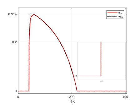
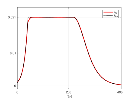
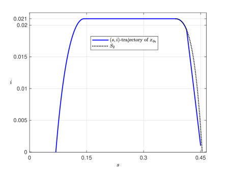
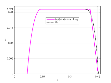
Figure 4. Solutions for the constant initial condition $\phi_{0}(t)\equiv x_{0}=(0.45,0.001)$. The dotted black lines in the pictures above represent the optimal control $u_{{bcp}}(t)$ and the value of $i_{{bcp}}(t)$, respectively, as computed by Bocop. The red lines represent the greedy control $u_{\phi_{0}}(t)=\beta-b_{\phi_{0}}(t)$ described in Theorem 4.5, and the $i$-component of the solution, respectively, computed with Matlab. In the pictures below, on the left, we plotted the trajectory of the solution $x_{\phi_{0}}$, corresponding to the greedy control $u_{\phi_{0}}$, with the curve $S_{2}$ in Theorem 4.5 plotted in dotted black line. On the right, the same plot for the solution $x_{{bcp}}$ corresponding to the control $u_{{bcp}}$.

5. Examples and numerical simulations

In the sequel, with the aid of numerical examples, we illustrate the greedy control schemes introduced in the previous section (Theorem 4.5 and Theorem 4.18).

Example 5.1.

The epidemic parameters we are choosing in this example are compatible with the state of knowledge of the COVID-19 epidemic in Italy in autumn 2021 (see [16], Example 4.3). Actually, we specialize (1.1) by choosing $\gamma=0.0714$, $\beta=0.5$, $i_{M}=0.021$, $\beta_{\star}=0.186$. An appropriate latency period would be between $4$ and $6$ ([28, 30, 40]). We consider here a delay $h=6$, which is large enough to appreciate the effect of the delay in numerical computations.

We start by considering a constant initial condition $\phi_{0}(t)\equiv x_{0}:=(s_{0},i_{0}):=(0.45,0.001)$ for all $t\in[-h,0]$. This choice represents the case in which there is an isolated-in-time spreading event at time $-h$; then, nothing happens ($s$ and $i$ stay constant) till time $0$ after which the infection can be transmitted.

Since $h\max\{\beta,\gamma\}\geq 1$, for every $L>0$ satisfying (4.21) we have $Lh\geq i_{M}$. By Theorem 4.17 (1), this implies that the control strategy described in Subsection 4.2 is equivalent to the one introduced in Subsection 4.1. Roughly speaking, the delay parameter $h=6$ is large enough to prevent any gain in imposing the Lipschitz condition in Assumption 4.9. We thus consider the “greedy” control policy $\widetilde{b}_{\phi_{0}}$ described in Theorem 4.5. This is possible, since it can be verified that $\phi_{0}$ belongs to viable set $\mathcal{B}$ (see Theorem 4.2).

The numerical computation of the greedy control $u_{\phi_{0}}(t):=\beta-\widetilde{b}_{\phi_{0}}(t)$ and the corresponding solution $x_{\phi_{0}}=(s_{\phi_{0}},i_{\phi_{0}})$ are performed in Matlab and plotted in red in Figure 4. In the same figure, we compare the performance of this control strategy with the “optimal” one numerically obtained by the algorithmic optimal control toolbox Bocop ([36]), and denoted by $u_{bcp}$. The latter is obtained by choosing the Gauss’s II method and a discretization detail of 10 time steps per day. It can be observed that the two control actions appear to be close one to the other. On the other hand, it can be noted that $u_{\phi_{0}}$ starts its action earlier with respect to $u_{bcp}$, as illustrated in zoomed detail inside the small bottom-right box of Figure 4. Moreover, differently from the optimal one $u_{bcp}$, the control strategy $u_{\phi_{0}}$ does not provide any time interval at the maximum regime $\beta_{\star}$ (corresponding to a lockdown policy), according to what already expected in Remark  4.6 (2).

The suboptimality of $u_{\phi_{0}}$ is also highlighted by the numerical computation of the costs. Considering for simplicity $G\equiv\text{Id}$ in (4.14), it reads

$$J(u_{\phi_{0}})=\int_{0}^{+\infty}u_{\phi_{0}}(t)\,dt=\int_{0}^{+\infty}\beta-b_{\phi_{0}}(t)\,dt,$$ (5.1)

and Matlab returns the value $J(u_{\phi_{0}})=38.766$, while Bocop gives $J(u_{{bcp}})=38.5263$.

It is worth noting also that, while Bocop provides an approximated optimal solution in some minutes, the computation time of the suboptimal greedy strategy with Matlab is of the order of a couple of seconds.

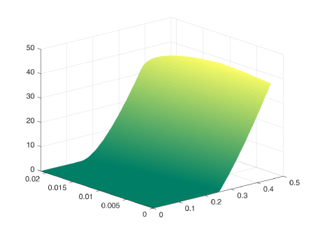
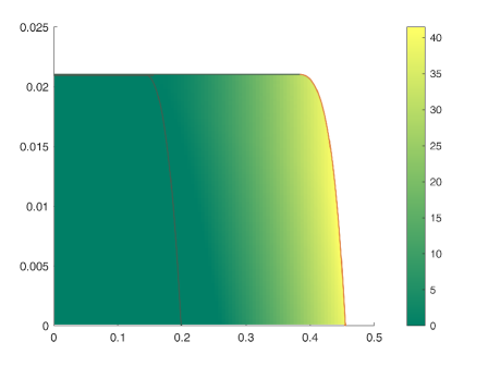
Figure 5. The value of the cost $J$ for different constant initial conditions in $B$. On the right, the viable zone $B$ of the $(s,i)$-plane is represented, with different colors for different values of $J$. The color scale goes from dark green, corresponding to a null cost, to light yellow corresponding to the highest values. The curve in black, crossing the set $B$, represents the relative boundary ($\Gamma_{\beta}$) of the set $A$. On the left, the 3D graph of the map $x\mapsto J(x)$.

In order to further analyze the effectiveness and performance of the greedy control strategy, in Figure 5 we plot the function $x\mapsto\bar{J}(x):=J(u_{\phi_{x}})$ by considering constant initial conditions $\phi_{x}(t)\equiv x$ in $[-h,0]$, for $x\in B$, and where $u_{\phi_{x}}=\beta-b_{\phi_{x}}$ with $b_{\phi_{x}}$ defined in (4.18). As expected, the value of $\bar{J}(x)$ is $0$ when $x\in A$, while $J$ increases in value as the initial condition approaches the set $S_{1}\cup S_{2}\subset\partial B$ (using the notation in Theorem 4.2, see also Figure 1).

We then apply the greedy control policy described in Theorem 4.5 to different initial conditions (reaching the same point $x_{0}=(0.45,0.001)\in T$ at time $0$). This allows us to evaluate the dependence of the control, the corresponding solution and the corresponding cost, on the past/delayed behaviour of the initial condition.

We first consider the situation in which at time $t=-h$ there is an initial proportion of exposed population that is not infectious, but it is recovering with rate equal to $\gamma$. We thus consider $\phi_{1}:[-h,0]\to\mathbb{R}^{2}$ defined by

$$\phi_{1}(t)=(s_{0},i_{0}e^{-\gamma t}),\quad t\in[-h,0].$$ (5.2)

The constancy of the $s$-component of the initial condition can be assumed without loss of generality, because the dynamics in system (1.1) does not depend on the delayed value of $s$. It can be numerically verified that $\phi_{1}\in\mathcal{B}$, and thus the control introduced in Theorem 4.5 is feasible also for this initial condition. The control $u_{\phi_{1}}$ and the corresponding $i$-component of the solution, $i_{\phi_{1}}$, are depicted in Figure 6.

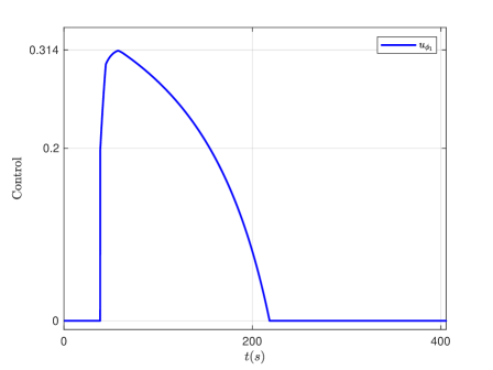
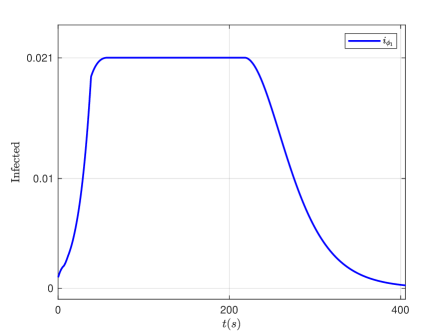
Figure 6. The control $u_{\phi_{1}}$ obtained, via Theorem 4.5, for the initial condition $\phi_{1}$ defined in (5.2), and the corresponding infected population $i_{\phi_{1}}$.

Compared to the constant initial condition case depicted in Figure 4, we note that we have a slightly “perturbed behaviour” of the $i$-component in the first time steps, due to the greater value of the initial condition in $[-h,0]$. Besides this slight discrepance in the very short term, the proposed feedback control $u_{\phi_{1}}$ and the corresponding behaviour of the solution are qualitatively equivalent to the ones obtained with the constant initial condition $\phi_{0}$. Also the cost $J(\phi_{1})=38.799$ is again close to the cost $J(\phi_{0})$ corresponding to the constant initial condition.

We finally consider a third initial condition motivated by mathematical interest. We take $\phi_{2}:[-h,0]\to\mathbb{R}^{2}$ defined by

$$\phi_{2}(t)=(s_{0},i_{0}+\frac{i_{M}-i_{0}}{1-e^{-5h}}(1-e^{5t})),\quad t\in[-h,0],$$ (5.3)

i.e., we consider an exponentially decreasing $i$-component, starting at $i=i_{M}$ at $t=-h$ and reaching $i=i_{0}$ at $t=0$. The function $i_{\phi_{2}}:[-h,0]\to\mathbb{R}$ is illustrated in Figure 7, and it models an initial condition close to the “worst case” used in the proof of Theorem 4.5: it remains close to the maximal admissible $i_{M}$ before rapidly decreasing to the initial value $i_{0}$.

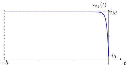
Figure 7. The $i$-component of $\phi_{2}$ defined in (5.3), in the interval $[-h,0]$.

The resulting solution and control are depicted in Figure 8.

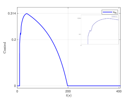
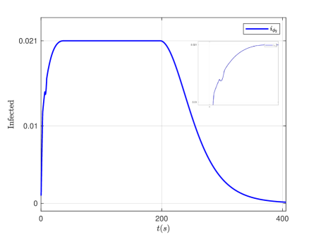
Figure 8. The control $u_{\phi_{2}}$ obtained, via Theorem 4.5, for the initial condition $\phi_{2}$ defined in (5.3), and the corresponding infected population $i_{\phi_{2}}$. In the upper-right squares, we highlight the non-monotonic behaviour of $u_{\phi_{2}}$ and $i_{\phi_{2}}$ in the initial part of the epidemic horizon.

With respect to the previous cases of Figure 4 and Figure 6, we note that we have an initial non-monotonic evolution of the $i$-component and of the control $u_{\phi_{2}}$. We also note that the control action starts earlier, since the solution reaches earlier the curve $S_{2}$ defined in Theorem 4.5 (as can be numerically verified). This discrepancy is also reflected by the value $J(\phi_{2})=41.004$, which is larger than the costs corresponding to the initial conditions $\phi_{0}$ and $\phi_{1}$ previously computed.

6. Conclusions

This paper is concerned with a viability analysis and control synthesis of a delayed SIR model under an ICU state-constraint, where a constant delay represents an incubation/latency time. As a by-product of the considered functional viability tools, we provided feasible feedback control maps driving the solutions to a safe set, according to a cost functional to be minimized. Two scenarios were examined: in the first the initial conditions are simply continuous, while in the other they satisfy a suitable Lipschitz continuity assumption. In the latter case, we studied the dependence of the obtained results on the delay parameter. The theoretical developments have been illustrated via a numerical example inspired by the recent COVID-19 epidemic.

Appendix A Technical Proofs

In this Appendix we collect some technical results.

Lemma A.1.

Assume that $\widetilde{F}(\phi)\in\mathcal{D}_{\mathcal{B}}(\phi)$ for any $\phi\in\mathcal{B}$. Then, there exists a solution $x_{\phi}$ to the Cauchy problem (4.17). Moreover, any maximal solution is global, i.e., $\text{dom}(x_{\phi})=[-h,+\infty)$, for all $\phi\in\mathcal{B}$, and it holds that $S(t)x_{\phi}\in\mathcal{B},\;\;\forall t\in\mathbb{R}_{+}$. A similar result holds when $\mathcal{B}$ is replaced by $\mathcal{B}_{L,h}$, and $\widetilde{F}$ is replaced by $F_{L,h}$.

Proof.

To prove the existence of solutions, we consider first a convex regularization of the (possibly discontinuous) map $\widetilde{F}:\mathcal{B}\to\mathbb{R}^{2}$, by considering the set-valued map $\widetilde{G}:\mathcal{B}\rightsquigarrow\mathbb{R}^{2}$, defined by

$$\widetilde{G}(\phi)=\begin{cases}\{\widetilde{F}(\phi)\}=\{f(\phi,\beta)\},&\text{ if }\phi(0)\in B\setminus(S_{1}\cup S_{2}),\\ \text{co}\left\{f(\phi,\beta),\widetilde{F}(\phi)\right\},&\text{ if }\phi(0)\in S_{1}\cup S_{2}.\end{cases}$$ (A.1)

Note that if $\phi(0)\in S_{1}$, we can also write $\widetilde{G}(\phi)=\text{co}\{f(\phi,\beta),f(\phi,\min\{\beta,\frac{\gamma i_{M}}{s_{\phi}(0)i_{\phi}(-h)}\})\}$, while, if $\phi(0)\in S_{2}$ we have $\widetilde{G}(\phi)=\text{co}\{f(\phi,\beta),f(\phi,\min\{\beta,\beta_{\star}\frac{i_{M}}{i_{\phi}(-h)}\})\}$. The map $\widetilde{G}:\mathcal{B}\rightsquigarrow\mathbb{R}^{2}$ is obtained by considering the Krasovskii regularization (see [23, Definition 2.2] for the definition for finite dimensional maps) of the $\widetilde{F}:\mathcal{B}\to\mathbb{R}^{2}$ in $\mathcal{B}$, defined by

$$\widetilde{G}(\phi)=\bigcap_{\varepsilon>0}\text{co}\{\widetilde{F}(\varphi)\;\;|\;\varphi\in\mathds{B}_{\infty}(\phi,\varepsilon)\cap\mathcal{B}\},$$

where $\mathds{B}_{\infty}(\phi,\varepsilon):=\{\varphi\in\mathcal{C}\;|\;\sup_{t\in[-h,0]}|\varphi(t)-\phi(t)|_{\max}\leq\varepsilon\}$. By definition, $\widetilde{G}:\mathcal{B}\to\mathbb{R}^{2}$ has non-empty, compact and convex values, and $\widetilde{F}(\phi)\in\widetilde{G}(\phi)$ for all $\phi\in\mathcal{B}$. We now prove that $\widetilde{G}$ is also upper semicontinuous, i.e.,

$$\forall\,\phi\in\mathcal{B},\;\forall\;\varepsilon>0\;\exists\,\delta>0\text{ such that }\varphi\in\mathds{B}_{\infty}(\phi,\delta)\cap\mathcal{B}\;\Rightarrow\;\widetilde{G}(\varphi)\subseteq\widetilde{G}(\phi)+B_{|\cdot|_{\max}}(0,\varepsilon).$$

Let us take $\phi\in\mathcal{B}$ and proceed by cases.

1. If $\phi(0)\in B\setminus(S_{1}\cup S_{2})$, the conclusion easily follows by observing that $\widetilde{G}(\phi)=\{f(\phi,\beta)\}$, the map $f(\cdot,\beta):\mathcal{B}\to\mathbb{R}^{2}$ is continuous with respect to $\|\cdot\|_{\infty}$ in $\mathcal{B}$ and the set $B\setminus(S_{1}\cup S_{2})$ is relatively open in $B$.

2. If $\phi(0)\in S_{1}\setminus S_{2}$, we distinguish the following two sub-cases.

   1. If $i_{\phi}(-h)=0$, there exists $\delta>0$ such that, if $\|\varphi-\phi\|_{\infty}\leq\delta$ then

      $${\beta\leq\frac{\gamma i_{M}}{(\frac{\gamma}{\beta_{\star}}+\delta)\delta}\leq}\frac{\gamma i_{M}}{s_{\varphi}(0)i_{\varphi}(-h)},$$

      and thus $b(\varphi)=\beta$, implying $\widetilde{G}(\varphi)=\{f(\varphi,\beta)\}$, and concluding the proof in this case.

   2. In the case $i_{\phi}(-h)>0$, we note that for any $\varepsilon^{\prime}>0$ there exists $\delta^{\prime}>0$ such that $\|\phi-\varphi\|_{\infty}\leq\delta^{\prime}$ implies

      $$\Big{|}\frac{\gamma i_{M}}{s_{\phi}(0)i_{\phi}(-h)}-\frac{\gamma i_{M}}{s_{\varphi}(0)i_{\varphi}(-h)}\Big{|}\leq\varepsilon^{\prime}.$$

      Given $\varepsilon>0$, by continuity of $f:\mathcal{C}\times U\to\mathbb{R}^{2}$, of the $\min$ operator, and by the previous inequality, there exists a $\delta>0$ such that $\|\phi-\varphi\|_{\infty}\leq\delta$ implies

      $$\widetilde{G}(\varphi) =\text{co}\{f(\varphi,\beta),f(\varphi,\min\{\beta,\frac{\gamma i_{M}}{s_{\varphi}(0)i_{\varphi}(-h)}\})\}$$

      $$\subseteq\text{co}\left\{f(\phi,\beta)+B_{|\cdot|_{\max}}(0,\varepsilon),f(\phi,\min\{\beta,\frac{\gamma i_{M}}{s_{\phi}(0)i_{\phi}(-h)}\}+B_{|\cdot|_{\max}}(0,\varepsilon)\right\}$$

      $$=\text{co}\{f(\phi,\beta),f(\phi,\min\{\beta,\frac{\gamma i_{M}}{s_{\phi}(0)i_{\phi}(-h)}\})\}+B_{|\cdot|_{\max}}(0,\varepsilon)=\widetilde{G}(\phi)+B_{|\cdot|_{\max}}(0,\varepsilon),$$

      where we used the fact that, for any $z_{1},z_{2}\in\mathbb{R}^{n}$ and any convex set $K\subset\mathbb{R}^{n}$ it holds that

      $$\text{co}\{z_{1}+K,z_{2}+K\}=\text{co}\{z_{1},z_{2}\}+K.$$

      We have thus proved the upper semicontinuity in this case.

3. Let $\phi(0)\in S_{2}\setminus S_{1}$. The case $i_{\phi}(-h)=0$ can be treated as in the previous case. If $i_{\phi}(-h)>0$, the claim follows by continuity of the function $i\mapsto\beta_{\star}\frac{i_{M}}{i}$ when $i\neq 0$, by adapting the argument of the previous case.

4. For $\phi(0)\in S_{1}\cap S_{2}=\{(\frac{\gamma}{\beta_{\star}},i_{M})\}$, it suffices to recall that in this case we have

   $$\frac{\gamma i_{M}}{s_{\phi}(0)i_{\phi}(-h)}=\beta_{\star}\frac{i_{M}}{i_{\phi}(-h)},$$

   and the same continuity argument can thus be applied.

Summarizing, the set-valued map $\widetilde{G}:\mathcal{C}\to\mathbb{R}^{n}$ is upper semicontinuous with non-empty, compact and convex values. By assumption, $\widetilde{F}(\phi)\in\mathcal{D}_{\mathcal{B}}(\phi)$ for all $\phi\in\mathcal{B}$. Since $\widetilde{F}(\phi)\in\widetilde{G}(\phi)$ for all $\phi\in\mathcal{B}$, this implies

$$\widetilde{G}(\phi)\cap D_{\mathcal{B}}(\phi)\neq\varnothing\quad\forall\,\phi\in\mathcal{B}.$$

We can thus apply [18, Theorem 1.1] (which is the local version of Theorem 2.7) proving that, for any $\phi\in\mathcal{B}$ there exist a $\tau>0$ and a function $x_{\phi}:[-h,\tau)\to\mathbb{R}^{2}$ satisfying

$$x^{\prime}_{\phi}(t)\in\widetilde{G}(S(t)x_{\phi})\ \text{ for a.e.\ }t\in[0,\tau),$$ (A.2)

$$S(0)x_{\phi}=\phi,$$

$$S(t)x_{\phi}\in\mathcal{B}\ \ \forall\,t\in[0,\tau).$$

The fact that $\tau=+\infty$, i.e. that maximal solutions are defined on $[-h,+\infty)$, follows again by viability analysis, since $B$ is compact and thus solutions cannot explode in finite time, see [18, Page 12, Proof of Theorem 1.1].

To conclude the proof we show that, for any $\phi\in\mathcal{B}$, the only viable direction in $\widetilde{G}(\phi)$ is given by the vector $\widetilde{F}(\phi)$, that is

$$\{\widetilde{F}(\phi)\}=\widetilde{G}(\phi)\cap D_{\mathcal{B}}(\phi)\ \forall\,\phi\in\mathcal{B},$$ (A.3)

thus proving that any solution to (A.2) is a solution to (4.17).

By definition of $\widetilde{G}$ (see (A.1) and the two lines after) the claim is trivially true if, either,

• $\phi(0)\in B\setminus(S_{1}\cup S_{2})$, or

• $\phi(0)\in S_{1}$ and $\beta\leq\frac{\gamma i_{M}}{s_{\phi}(0)i_{\phi}(-h)}$, or

• $\phi(0)\in S_{2}$ and $\beta\leq\beta_{\star}\frac{i_{M}}{i_{\phi}(-h)}$.

We then proceed by analyzing the following two remaining cases, only. To this aim it is useful to note that, by Lemma 2.5, the claimed proposition (A.3) is equivalent to

$$\{\widetilde{F}(\phi)\}=\widetilde{G}(\phi)\cap T_{\mathcal{B}}(\phi(0))\ \forall\,\phi\in\mathcal{B}.$$ (A.4)

1. Let $\phi(0)\in S_{1}$ and $\beta>\frac{\gamma i_{M}}{s_{\phi}(0)i_{\phi}(-h)}$. Considering the vector $v=(0,1)$, normal to $B$ at $\phi(0)$, and recalling (2.1), we have

   $$\langle v,f(\phi,\frac{\gamma i_{M}}{s_{\phi}(0)i_{\phi}(-h)})\rangle=0,$$

   and

   $$\langle v,f(\phi,\beta)\rangle=\beta s_{\phi}(0)i_{\phi}(-h)-\gamma i_{\phi}(0)>0.$$

   Hence, by convexity, $\langle v,g\rangle>0$ for all $g\in\widetilde{G}(\phi)$, $g\neq\widetilde{F}(\phi)$. This proves (A.4), and hence (A.3), in the current case.

2. If $\phi(0)\in S_{2}$ and $\beta>\beta_{\star}\frac{i_{M}}{i_{\phi}(-h)}$, we can argue as in the first part of the proof of Theorem 4.5, case (c). There, we proved that, denoted by $w\in\mathbb{R}^{2}$ the unique normal vector (modulo positive scalar multiplication) to $B$ at $\phi(0)$, it holds

   $$\langle w,f(\phi,b(\phi))\rangle=\langle w,f(\phi,\beta_{\star}\frac{i_{M}}{i_{\phi}(-h)})\rangle=0,$$

   and $\langle w,f(\phi,\beta)\rangle>0$. Now, by convexity, we have $\langle w,f\rangle>0$ for all $f\in\widetilde{G}(\phi)$, $f\neq\widetilde{F}(\phi)$, concluding the proof.

∎

Lemma A.2.

For any value of $\gamma>0$, $\beta>\beta_{\star}>0$, $0<i_{M}\leq 1$ and for any $h>0$, the functions $\Gamma_{\beta,L,h}:[\frac{\gamma}{\beta},\widehat{s}_{\beta,L,h})\to\mathbb{R}_{+}$ and $\Gamma_{\beta_{\star},L,h}:[\frac{\gamma}{\beta_{\star}},\widehat{s}_{\beta_{\star},L,h})\to\mathbb{R}_{+}$ defined in Subsection 4.2 are strictly decreasing and concave. Moreover, the sets $A_{L,h}$ and $B_{L,h}$ defined in Theorem 4.12 are convex.

Proof.

We recall that $\Gamma_{\beta,L,h}:[\frac{\gamma}{\beta},\widehat{s}_{\beta,L,h})\to\mathbb{R}$ is defined as the graph in the plane $(s,i)$ of the solution of (4.24) with initial condition $(s(0),i(0))=(\frac{\gamma}{\beta},i_{M})$. Since $s\psi_{L,h}(i)>0$ for all $s\in[\frac{\gamma}{\beta},\widehat{s}_{\beta,L,h})$ and $i\in[0,+\infty)$, we can divide the equations in (4.24) by this quantity, obtaining that $\Gamma_{\beta,L,h}$ is solution to the differential equation

$$\frac{d}{ds}\,i(s)=-1+\frac{\gamma i(s)}{\beta s\psi_{L,h}(i(s))},$$

with initial condition $i(\frac{\gamma}{\beta})=i_{M}$, in the interval $[\frac{\gamma}{\beta},\widehat{s}_{\beta,L,h})$. For simplicity, in what follows we write $\Gamma_{\beta,L,h}(s):=i(s)$, for all $s\in[\frac{\gamma}{\beta},\widehat{s}_{\beta,L,h})$.

First we note that $\frac{di}{ds}(\frac{\gamma}{\beta})=0$ and

$$\frac{d^{2}i}{ds^{2}}(\frac{\gamma}{\beta})=-\frac{1}{\gamma}<0.$$

This implies that $i$ is strictly decreasing in a right-neighborhood $N$ of $s(0)=\frac{\gamma}{\beta}$ and, hence, $i(s)=\Gamma_{\beta,L,h}(s)<i_{M}$ for all $s\in N$. On the other hand, as long as $i\leq i_{M}$ and $s>\frac{\gamma}{\beta}$, we have

$$\frac{di}{ds}(s)\leq-1+\frac{\gamma}{\beta s}<0,$$

since $\frac{i}{\psi_{L,h}(i)}\leq 1$ for all $i\leq i_{M}$. This implies that $i$ is strictly decreasing in $[\frac{\gamma}{\beta},\widehat{s}_{\beta,L,h})$, and by definition of $\widehat{s}_{\beta,L,h}$ we also have that $i(s)>0$ for all $s\in[\frac{\gamma}{\beta},\widehat{s}_{\beta,L,h})$. We now show that its derivative is also decreasing, proving concavity. By definition of $\psi_{L,h}(i(s))$, we have

$$\frac{i(s)}{\psi_{L,h}(i(s))}=\begin{cases}\frac{i(s)}{i_{M}},\;\;\;&\text{if }i_{M}-Lh\leq i(s)\leq i_{M},\\[4.30554pt] \frac{i(s)}{i(s)+Lh},\;\;\;&\text{if }0\leq i(s)\leq i_{M}-Lh.\end{cases}$$

We note that both the functions $z\mapsto\frac{z}{i_{M}}$ and $z\mapsto\frac{z}{z+Lh}$ are strictly increasing in $[0,+\infty)$; since we have proved that $i(s)$ is strictly decreasing in $[\frac{\gamma}{\beta},\widehat{s}_{\beta,L,h})$, so is $s\mapsto\frac{i(s)}{\psi_{L,h}(i(s))}$. Then the function

$$s\mapsto\frac{di}{ds}(s)=-1+\frac{\gamma i(s)}{\beta s\psi_{L,h}(i(s))},$$

is also decreasing, concluding the proof of concavity of $\Gamma_{\beta,L,h}$ in $[\frac{\gamma}{\beta},\widehat{s}_{\beta,L,h})$.

The set $A_{L,h}$ defined in (4.27) is then convex, since defined as the intersection of the convex set $T$ with the hypo-graph of a concave function.

The proof for $\Gamma_{\beta_{\star},L,h}:[\frac{\gamma}{\beta_{\star}},\widehat{s}_{\beta_{\star},L,h})\to\mathbb{R}_{+}$ is similar. ∎

Lemma A.3.

Given an interval $I=[0,\tau)$ (with, possibly, $\tau=+\infty$), consider a continuous function $g:\mathbb{R}^{n}\to\mathbb{R}^{n}$ and $x_{0}\in\mathbb{R}^{n}$. Suppose there exists $x:I\to\mathbb{R}^{n}$, solution to

$$x^{\prime}(t)=g(x(t)),\;\;\;\;x(0)=x_{0},$$

and that there exists a compact set $Q\subset\mathbb{R}^{n}$ such that $x(t)\in Q$ for all $t\in I$. For a given $a>0$, for any $h\in(0,a)$ consider $g_{h}:\mathbb{R}^{n}\to\mathbb{R}^{n}$ such that:

• $g_{h}$ is uniformly converging to $g$ in $Q$, as $h\to 0$,

• $g_{h}$ are uniformly locally Lipschitz, i.e., for any compact set $K\subset\mathbb{R}^{n}$ there exists $M_{K}\geq 0$ such that

  $$|g_{h}(x_{1})-g_{h}(x_{2})|\leq M_{K}|x_{1}-x_{2}|,\;\;\;\forall h\in(0,a),\;\forall x_{1},x_{2}\in K.$$ (A.5)

• $g_{h}$ are uniformly sublinear in norm, i.e., there exist $A>0,B>0$ such that

  $$|g_{h}(x)|\leq A|x|+B,\;\;\;\forall h\in(0,a),\;\forall\,x\in\mathbb{R}^{n}.$$ (A.6)

Let us denote by $y_{h}:I\to\mathbb{R}^{n}$ the solution to

$$y^{\prime}(t)=g_{h}(y(t)),\;\;\;y(0)=x_{0}.$$

Then we have

$$\lim_{h\to 0^{+}}|x(t)-y_{h}(t)|=0\;\;\;\forall\;t\in I.$$

Moreover, for every compact interval $J\subset I$, there exists a sequence $h_{n}\to 0$ such that $y_{h_{n}}$ converges uniformly to $x$ on $J$.

Proof.

Let us fix $t\in I$. By (A.6), using Grönwall’s inequality (see [37, Lemma 2.7]) we have that

$$|y_{h}(t)|\leq\bar{R}:=|x_{0}|e^{At}+\frac{B}{A}(e^{At}-1),\,\;\forall h\in(0,a).$$ (A.7)

Given the compact set $K=Q\cup B_{\|\cdot\|}(0,\bar{R})$, consider $M_{K}>0$ as in (A.5). Now, for all $h\in(0,a)$, we have

$$|y_{h}(t)-x(t)| \leq\int_{0}^{t}|g_{h}(y_{h}(\theta))-g(x(\theta))|\,d\theta$$

$$\leq\int_{0}^{t}|g_{h}(y_{h}(\theta))-g_{h}(x(\theta))|\,d\theta+\int_{0}^{t}|g_{h}(x(\theta))-g(x(\theta))|\,d\theta$$

$$\leq M_{K}\int_{0}^{t}|y_{h}(\theta)-x(\theta)|\,d\theta+\int_{0}^{t}|g_{h}(x(\theta))-g(x(\theta))|\,d\theta$$

By uniform convergence, for every $\varepsilon>0$ there exists $\overline{h}\in(0,a)$ such that, for any $h\leq\overline{h}$, it holds that (recall that $t$ is fixed)

$$|y_{h}(t)-x(t)|\leq M_{K}\int_{0}^{t}|y_{h}(\theta)-x(\theta)|\,d\theta+\varepsilon.$$

Applying again the Grönwall’s Inequality ([37, Lemma 2.7]) this implies that

$$|y_{h}(t)-x(t)|\leq\varepsilon e^{M_{K}t}.$$

We have, thus, proved that

$$\lim_{h\to 0}|y_{h}(t)-x(t)|=0,$$

as required. Let us now take a compact subinterval $J\subset I$. By (A.7), the functions $y_{h}$ are uniformly bounded on $J$, i.e., there exists $C>0$ such that $|y_{h}(t)|\leq C$ for all $h\in(0,a)$ and for all $t\in J$. Moreover, by (A.6) we have $|g_{h}(t)|\leq AC+B$ for all for all $h\in(0,a)$ for all $t\in J$. In other words, the derivatives of the functions $y_{h}$ are uniformly bounded in $J$ and this implies that the functions $y_{h}$ are equicontinuous on $J$. By Ascoli-Arzelà’s theorem, there exists a subsequence $y_{h_{n}}$ that uniformly converges on $J$. By the pointwise convergence proven above, we then have $y_{h_{n}}\to x$ uniformly on $J$, concluding the proof. ∎

Acknowledgements. DB is member of GNCS-INdAM. LF is member of GNAMPA–INdAM.

References

- [1] F. E. Alvarez, D. Argente, and F. Lippi. A simple planning problem for COVID-19 lockdown. Technical report, National Bureau of Economic Research, 2020.
- [2] R. M. Anderson, B. Anderson, and R. M. May. Infectious diseases of humans: dynamics and control. Oxford university press, 1992.
- [3] J.-P. Aubin. Viability Theory. Birkhäuser Boston, Boston, MA, 2009.
- [4] F. Avram, L. Freddi, and D. Goreac. Optimal control of a SIR epidemic with ICU constraints and target objectives. Appl. Math. Comput., 418:126816, 2022.
- [5] F. Avram, L. Freddi, D. Goreac, J. Li, and J. Li. Controlled compartmental models with time-varying population: normalization, viability and comparison. J. Optim. Theory Appl., 198(3):1019–1048, 2023.
- [6] H. Behncke. Optimal control of deterministic epidemics. Optim. Control Appl. Methods, 21(6):269–285, 2000.
- [7] E. Beretta and Y. Takeuchi. Global stability of an SIR epidemic model with time delays. J. Math. Biol., 33(3):250–260, 1995.
- [8] A. Boccia and R. B. Vinter. The maximum principle for optimal control problems with time delays. SIAM J. Control Optim., 55(5):2905–2935, 2017.
- [9] H. Brezis. Functional analysis, Sobolev spaces and partial differential equations. Universitext. Springer, New York, 2011.
- [10] G. Buttazzo. Semicontinuity, relaxation and integral representation in the calculus of variations, volume 207 of Pitman Research Notes in Mathematics Series. Longman Scientific & Technical, Harlow; copublished in the United States with John Wiley & Sons, Inc., New York, 1989.
- [11] A. Di Liddo. A S-I-R vector disease model with delay. Math. Modelling, 7(5-8):793–802, 1986.
- [12] H. Frankowska and I. Haidar. Viable trajectories for nonconvex differential inclusions with constant delay. IFAC-PapersOnLine, 51(14):112–117, 2018. 14th IFAC Workshop on Time Delay Systems TDS 2018.
- [13] H. Frankowska, E. M. Marchini, and M. Mazzola. A relaxation result for state constrained inclusions in infinite dimension. Math. Control Relat. Fields, 6(1):113–141, 2016.
- [14] H. Frankowska, E. M. Marchini, and M. Mazzola. Necessary optimality conditions for infinite dimensional state constrained control problems. J. Differential Equations, 264(12):7294–7327, 2018.
- [15] L. Freddi. Optimal control of the transmission rate in compartmental epidemics. Math. Control Relat. Fields, 12(1):201–223, 2022.
- [16] L. Freddi and D. Goreac. Infinite horizon optimal control of a SIR epidemic under an ICU constraint. J. Convex Anal., 31(4), 2024.
- [17] L. Freddi, D. Goreac, J. Li, and B. Xu. SIR epidemics with state-dependent costs and ICU constraints: a Hamilton-Jacobi verification argument and dual LP algorithms. Appl. Math. Optim., 86(2):Paper No. 23, 31, 2022.
- [18] G. Haddad. Monotone viable trajectories for functional differential inclusions. J. Differential Equations, 42(1):1–24, 1981.
- [19] G. Haddad. Functional viability theorems for differential inclusions with memory. Ann. Inst. H. Poincaré Anal. Non Linéaire, 1(3):179–204, 1984.
- [20] J. Hale and S.M.Verduyn Lunel. Introduction to Functional Differential Equations, volume 99 of Applied Mathematical Sciences. Springer New York, 1993.
- [21] E. Hansen and T. Day. Optimal control of epidemics with limited resources. J. Math. Biol., 62(3):423–451, 2011.
- [22] S. Hu and N. Papageorgiou. Delay differential inclusions with constraints. Proc. Amer. Math. Soc., 123(7):2141–2150, 1995.
- [23] O. Hájek. Discontinuous differential equations I, II. J. Differential Equations, 32(2):149–170, 1979.
- [24] M. Kantner and T. Koprucki. Beyond just “flattening the curve”: Optimal control of epidemics with purely non-pharmaceutical interventions. J. Math. Ind., 10(1):1–23, 2020.
- [25] W. O. Kermack and A. G. McKendrick. A contribution to the mathematical theory of epidemics. Proc. R. Soc. Lond. A, 115(772):700–721, 1927.
- [26] D. I. Ketcheson. Optimal control of an SIR epidemic through finite-time non-pharmaceutical intervention. J. Math. Biol., 83(1):7, 2021.
- [27] T. Kruse and P. Strack. Optimal control of an epidemic through social distancing. url=https://ssrn.com/abstract=3581295, 2020.
- [28] S. A. Lauer, K. H. Grantz, Q. Bi, F. K. Jones, Q. Zheng, H. R. Meredith, A. S. Azman, N. G. Reich, and J. Lessler. The incubation period of coronavirus disease 2019 (COVID-19) from publicly reported confirmed cases: Estimation and application. Ann. Intern. Med., 172(9):577–582, 2020. PMID: 32150748.
- [29] Z. Liu, P. Magal, O. Seydi, and G. Webb. A covid-19 epidemic model with latency period. Infect. Dis. Model., 5:323–337, 2020.
- [30] T. Ma, S. Ding, R. Huang, H. Wang, J. Wang, J. Liu, J. Wang, J. Li, C. Wu, H. Fan, and N. Zhou. The latent period of coronavirus disease 2019 with SARS-CoV-2 B.1.617.2 delta variant of concern in the postvaccination era. Immunity, Inflammation and Disease, 10(7):e664, 2022.
- [31] M. Martcheva. An introduction to mathematical epidemiology, volume 61. Springer, 2015.
- [32] C. C. McCluskey. Complete global stability for an SIR epidemic model with delay—distributed or discrete. Nonlinear Anal. Real World Appl., 11(1):55–59, 2010.
- [33] L. Miclo, D. Spiro, and J. Weibull. Optimal epidemic suppression under an ICU constraint: An analytical solution. J. Math. Econom., 101:102669, 2022.
- [34] B. Patterson and J. Wang. How does the latency period impact the modeling of COVID-19 transmission dynamics? Mathematics in Applied Sciences and Engineering, 3(1):60–85, 2022.
- [35] R. Rockafellar and R.-B. Wets. Variational Analysis, volume 317 of Gundlehren der mathematischen Wissenchaften. Springer-Verlag, Berlin, 3rd printing, 2009 edition, 1998.
- [36] I. S. Team Commands. Bocop: an open source toolbox for optimal control. http://bocop.org, 2017.
- [37] G. Teschl. Ordinary Differential Equations and Dynamical Systems. Graduate studies in Mathematics. American Mathematical Soc., 2012.
- [38] R. B. Vinter. State constrained optimal control problems with time delays. J. Math. Anal. Appl., 457(2):1696–1712, 2018.
- [39] R. B. Vinter. Optimal control problems with time delays: constancy of the Hamiltonian. SIAM J. Control Optim., 57(4):2574–2602, 2019.
- [40] Y. Wu, L. Kang, Z. Guo, J. Liu, M. Liu, and W. Liang. Incubation Period of COVID-19 Caused by Unique SARS-CoV-2 Strains: A Systematic Review and Meta-analysis. JAMA Network Open, 5(8), 2022.
- [41] C. Yang, Y. Yang, Z. Li, and L. Zhang. Modeling and analysis of COVID-19 based on a time delay dynamic model. Math. Biosci. Eng., 18(1):154–165, 2021.
- [42] H. Yang, X. Lin, and J. Wu. Qualitative analysis of a time-delay transmission model for COVID-19 based on susceptible populations with basic medical history. Qeios, 08 2023.
- [43] N. Yoshida and T. Hara. Global stability of a delayed SIR epidemic model with density dependent birth and death rates. J. Comput. Appl. Math., 201(2):339–347, 2007.
- [44] G. Zaman, Y. H. Kang, and I. H. Jung. Optimal treatment of an sir epidemic model with time delay. Biosystems, 98(1):43–50, 2009.