Unbounded quantum advantage in communication complexity measured by distinguishability

Abstract

Communication complexity is a pivotal element in information science, with quantum theory presenting a significant edge over classical approaches. The standard quantification of one-way communication complexity relies on the minimal dimension of the systems that the sender communicates to accomplish the designated task. In this study, we adopt a novel perspective, measuring the complexity of the communication by the distinguishability of the sender’s input without constraining the dimension of the communicated systems. This measure becomes especially pertinent when maintaining the confidentiality of the sender’s input is essential. After establishing the generic framework, we focus on two important categories of communication complexity tasks—the general version of random access codes and equality problems defined by graphs. We derive lower bounds on the distinguishability of the sender’s input as a function of the success metric of these tasks in classical communication. Notably, we show that the ratio between the distinguishability in classical and quantum communication to achieve the same success metric escalates with the complexity of these tasks, reaching arbitrarily large values. Besides, we demonstrate the quantum advantage by employing qubits in solving equality problems associated with odd-cycle graphs. Furthermore, we derive lower bounds on distinguishability for another class of communication tasks, namely, pair-distinguishability tasks, and present several instances of the quantum advantage.

I Introduction

Communication complexity stands as a cornerstone in information science, finding applications in diverse fields such as distributed computation, query complexity, game theory, integrated circuit design, cryptography, and streaming algorithms Kushilevitz and Nisan (2006); Roughgarden (2016); Rao and Yehudayoff (2020); Yao (1979). In its most fundamental form, communication tasks involve two entities—the sender and receiver—aiming to compute a function based on both of their inputs. The traditional measure for one-way communication complexity pertains to the minimal dimension of the systems that the sender communicates to fulfil the task. Remarkably, quantum theory demonstrates a substantial edge over classical methods in various tasks, as evidenced by the fact that the ratio between the dimensions of classical and quantum systems required to accomplish the given task can be arbitrarily large as the complexity of the task increases Raz ; Buhrman et al. (2010, 2001, 1998); de Wolf (2002); Buhrman et al. (2016); Saha and Chaturvedi (2019); Gupta et al. (2023).

In this study, we adopt a novel perspective on communication complexity. The distinguishability of the sender’s input is defined as the average probability of distinguishing the sender’s input from the communicated message, whether classical or quantum. This serves as our measure of complexity, with no limitations on the dimension of the communicated systems. The underlying concept is that the distinguishability of the sender’s input quantifies the extent to which information about the sender’s input is revealed. Therefore, a higher required distinguishability of the sender’s input corresponds to an increased amount of communication, and conversely, a lower minimum indicates a lower amount of communication. Moreover, accomplishing a communication task while maintaining minimal distinguishability of the sender’s input becomes crucial when the confidentiality of the sender’s input is a concern. Traditional communication complexity, measured by the dimension of the communicated systems, overlooks the privacy of the sender’s input. On the other hand, cryptography prioritizes communication privacy but does not inherently consider the complexity of the communication process Ekert (1991); Gisin et al. (2002). Our approach addresses both aspects within a unified framework.

To commence, we discuss the generic task of ‘communication complexity based on distinguishability’ and outline methodologies for determining the minimal distinguishability of the sender’s input concerning the success metric in both classical and quantum communication. To quantify the quantum advantage, we take the ratio between the minimum required distinguishability of the sender’s input in classical and quantum communication to achieve a specific success metric value of the task. Moving to the primary outcomes of our investigation, we examine two categories of communication complexity tasks with diverse applications. The first category involves the general version of random access codes (RAC), where the sender possesses a string of $d$its of size $n$, and the receiver seeks to guess a randomly chosen $d$it from that string Casaccino et al. (2008); Czechlewski et al. (2018). The second category is an equality problem defined by graphs, where the objective is to determine whether the sender’s input and the receiver’s inputs are the same or not, given that the inputs randomly occur according to a graph Gupta et al. (2023). We establish lower bounds on the distinguishability of the sender’s inputs as a function of the success metric and the specifications of the task (i.e., $d,n,$ for RAC, and the properties of the graph for the equality problem), in classical communication. We show that the ratio between distinguishability in classical and quantum communication to attain the same success metric increases with $d$ in RAC, and similarly, for Hadamard graphs Frankl and Rodl (1987), this ratio grows with the size of the graph. We provide a comprehensive study of quantum advantages for RAC with $d,n=2,3$, and equality problems for odd-cycle graphs. Furthermore, we present classical lower bounds on the distinguishability of the sender’s input for the pair-distinguishability task, a generalized version of the task introduced in Chaturvedi and Saha (2020). We demonstrate instances where quantum theory offers advantages. In conclusion, we offer insights into quantum advantage within communication complexity based on distinguishability and outline potential future research directions.

II communication complexity based on distinguishability

First, let us establish the notation $[K]$ to represent the set $\{1,\cdots,K\}$ for any positive integer $K$. In the one-way communication complexity task, Alice, the sender, is assigned an input variable $x$ sampled from the set $[N]$. The probability of obtaining $x$ is denoted by $p_{x}$, with $p_{x}=1/N$ for a uniform distribution. In each task iteration, based on the value of $x$, Alice transmits a message (either classical or quantum) to Bob, the receiver. Bob is also given an input variable $y\in[M]$, and depending on $y$ and the received message, he produces an output $z\in[D]$. Multiple rounds of this task are performed to collect frequency statistics represented by conditional probabilities $p(z|x,y)$. The objective is to maximize a success metric of the form:

$$\mathcal{S}=\sum_{x,y,z}c(x,y,z)p(z|x,y),$$ (1)

where $c(x,y,z)\geqslant 0$, and the metric is normalized by ensuring $\sum_{x,y,z}c(x,y,z)=1$ so that the maximum value of $\mathcal{S}$ is 1.

The communication complexity is subject to the constraint on the distinguishability of inputs $x$. The distinguishability probability is defined as the maximum average guessing probability of determining input $x$ from the message (classical or quantum) using the optimal strategy:

$$\mathcal{D}=\max_{M}\Bigg{\{}\sum_{x}p_{x}p(z=x|x,M)\Bigg{\}},$$ (2)

where $M$ denotes the best possible measurement. Allowing $\mathcal{D}$ to be 1 would enable Alice to simply transmit the input $x$ via classical $N$-dimensional systems, making the task trivial. The task becomes nontrivial when $\mathcal{D}$ is less than 1. It is important to note that the success metric is typically associated with guessing some function of $x$ and $y$, i.e.,

$$\mathcal{S}=\sum_{x,y}c(x,y)p(z=f(x,y)|x,y).$$ (3)

While the success metric (1) is general, all tasks demonstrating quantum advantage in this work are of the form (3). We will now find how this communication task translates into classical and quantum communication and what is meant by quantum advantage.

Classical communication

In classical communication, Alice sends $d-$labelled message $m\in[d]$ depending on the input $x$. Any encoding is described by probability distributions of sending $m$ given input $x$, $\{p_{e}(m|x)\}$, where $\sum_{m}p_{e}(m|x)=1$ for all $x$. Similarly, the generic strategy for providing Bob’s output is defined by the probability distributions of output $z$ given $m,y,$ denoted as $\{p_{d}(z|y,m)\}$, where $\sum_{z}p_{d}(z|y,m)=1$ for all $m,y$. It is important to note that there is no restriction on the dimension $d$, implying $m$ can take an arbitrarily large number of distinct values. Using this fact, it can be shown, as detailed in Chaturvedi and Saha (2020) (Observation 4), that sharing classical randomness is not beneficial for this task. For this generic classical encoding and decoding, the resulting probability is expressed as follows:

$$p(z|x,y)=\sum_{m}\sum_{x,y}p_{e}(m|x)p_{d}(z|y,m).$$ (4)

Let us obtain the expression of distinguishability of Alice’s input (2) given an encoding. By substituting the probabilities (4) into (2) and leveraging the property that the maximum value of any convex combination of a set of numbers is the maximum number from that set, we obtain

$$\mathcal{D}_{C} = \max_{\{p_{d}(z|m)\}}\sum_{m}\sum_{x}p_{x}p_{e}(m|x)p_{d}(z=x|m)$$ (5)

$$= \max_{\{p_{d}(z|m)\}}\sum_{m}\left(\sum_{x}p_{x}p_{e}(m|x)p_{d}(z=x|m)\right)$$

$$= \sum_{m}\max_{x}\bigg{\{}p_{x}p_{e}(m|x)\bigg{\}}.$$

For the uniform distribution $p_{x}=1/N$, the above simplifies to

$$\mathcal{D}_{C}=\frac{1}{N}\sum_{m}\max_{x}\bigg{\{}p_{e}(m|x)\bigg{\}}.$$ (6)

It turns out that the expression of the optimal value of the success metric (1) in classical communication, denoted by $\mathcal{S}_{C},$ can be expressed only in terms of encoding $\{p_{e}(m|x)\}$. By substituting (4) into (1) and using the fact that the maximum value of any convex combination of a set of numbers is the maximum number from that set, we find

$$\mathcal{S}_{C} = \max_{\{p_{e}(m|x)\},\{p_{d}(z|y,m)\}}\sum_{x,y,z}\sum_{m}c(x,y,z)p_{e}(m|x)p_{d}(z|y,m)$$ (7)

$$= \max_{\{p_{e}(m|x)\},\{p_{d}(z|y,m)\}}\sum_{y,z}\sum_{m}\left(\sum_{x}c(x,y,z)p_{e}(m|x)\right)p_{d}(z|y,m)$$

$$= \max_{\{p_{e}(m|x)\}}\sum_{y,m}\max\left\{\left(\sum_{x}c(x,y,z=1)p_{e}(m|x)\right),\cdots,\left(\sum_{x}c(x,y,z=D)p_{e}(m|x)\right)\right\}.$$

For the particular case of binary-outcome, $z\in[2]$, the above expression simplifies to

$$\mathcal{S}_{C} = \max_{\{p_{e}(m|x)\}}\left[1-\sum_{m,y}\min\left\{\sum_{x}c(x,y,z=1)p_{e}(m|x),\sum_{x}c(x,y,z=2)p_{e}(m|x)\right\}\right].$$ (8)

Quantum communication

In quantum communication, Alice transmits a quantum state $\rho_{x}$ acting on $\mathbbm{C}^{d}$, and Bob’s output is the result of a quantum measurement described by sets of positive semi-definite operators $\{M_{z|y}\}_{z,y}$, with $z\in[D],y\in[M]$, and $\sum_{z}M_{z|y}=\mathbbm{1}$. It is worth noting that the dimension of quantum systems, denoted as $d$, can take arbitrary values. This setup results in the following statistics:

$$p(z|x,y)=\text{Tr}(\rho_{x}M_{z|y}).$$ (9)

Consequently, the expression of distinguishability is given by,

$$\mathcal{D}_{Q}=\max_{\{M_{x}\}}\sum_{x}p_{x}\text{Tr}(\rho_{x}M_{x}).$$ (10)

Fact 1.

The distinguishability of $N$ quantum states that belong to $\mathbbm{C}^{d}$ sampled form uniform distribution $p_{x}=1/N$,

$$\mathcal{D}_{Q}\leqslant\frac{d}{N}.$$ (11)

For uniform distribution, the distinguishability of a given set of quantum states is given by

$$\mathcal{D}_{Q}=\max_{\{M_{x}\}}\frac{1}{N}\sum_{x}\text{Tr}(\rho_{x}M_{x})\leqslant\frac{1}{N}\sum_{x}\text{Tr}(M_{x})=\frac{d}{N}.$$ (12)

Here, we use the fact that the $\text{Tr}(\rho_{x})=1$, the definition of quantum measurement $M_{x}\geqslant 0,\sum_{x}M_{x}=\mathbbm{1}$.

Quantifying Quantum Advantage

In this work, our objective is to measure the quantum advantage in communication complexity with respect to the distinguishability of $x$. Quantum advantage is established when, to achieve a given value of a success metric $\mathcal{S}$, the minimum value of classical distinguishability $\mathcal{D}_{C}$ surpasses the minimum value of quantum distinguishability $\mathcal{D}_{Q}$. To quantify this, we draw an analogy from the standard notion of communication complexity and consider the ratio of the distinguishability in classical and quantum communication, $\mathcal{D}^{\mathcal{S}}_{C}/\mathcal{D}^{\mathcal{S}}_{Q}$, given that the success metric attains at least a certain value, $\mathcal{S}$, in both, classical and quantum communication. If this ratio exceeds 1, it indicates a quantum advantage. In particular, we aim to derive a relationship of the following form:

$$\mathcal{F}(\mathcal{S}_{C})\leqslant\mathcal{D}_{C}$$ (13)

where $\mathcal{F}(\mathcal{S}_{C})$ is some function on $\mathcal{S}_{C}$ and specifications of the task. This enables us to establish a lower bound on $\mathcal{D}_{C}$ given a value of $\mathcal{S}$. Subsequently, we present quantum communication protocols achieving the same value $\mathcal{S}$ such that $\mathcal{D}_{Q}$ is less than the obtained lower bound on $\mathcal{D}_{C}$. The advantage is considered unbounded if the ratio $\mathcal{D}^{\mathcal{S}}_{C}/\mathcal{D}^{\mathcal{S}}_{Q}$ can become arbitrarily large.

Additionally, the quantum advantage can be quantified in the reverse direction by determining the ratio between the success metric, $\mathcal{S}^{\mathcal{D}}_{Q}/\mathcal{S}^{\mathcal{D}}_{C}$, under the condition that the distinguishability cannot be greater than the value, $\mathcal{D}$, in both, quantum and classical communication. The existence of such advantage, termed as ‘communication tasks under bounded distinguishability’, was first demonstrated in Chaturvedi and Saha (2020). Similar types of communication tasks are explored in Tavakoli et al. (2022) under the name ‘informationally restricted correlations’.

III Random access codes

In this task, Alice is provided with a string of $n$ dits, denoted as $x=x_{1}x_{2}\cdots x_{n}$, randomly selected from the set encompassing all possible strings. Each $x_{y}$ in the string belongs to the set $[d]$ for all $y\in[n]$. During communication, Alice conveys information about the acquired string using either classical or quantum systems. Bob’s task is to deduce the $y$-th dit, with $y$ being randomly chosen from the set $[n]$. The success metric is determined by the average success probability, defined through

$$\mathcal{S}(n,d)=\frac{1}{nd^{n}}\sum_{x,y}p(z=x_{y}|x,y).$$ (14)

Here the task is uniquely defined by the values of $n$ and $d$. Utilizing (7), we can express the distinguishability for any specific encoding as follows:

$$\mathcal{D}_{C}=\frac{1}{d^{n}}\sum_{m}\max_{x}\bigg{\{}p_{e}(m|x)\bigg{\}}.$$ (15)

Theorem 1.

For any $n$ and $d$, the following holds in classical communication

$$n\mathcal{S}_{C}(n,d)+1-n\leqslant\mathcal{D}_{C}.$$ (16)

Proof.

First, we express this average success metric (14) in terms of the general form of success metric (1) as

$$c(x,y,z)=\frac{1}{nd^{n}}\times\begin{cases}1,&\text{if $z=x_{y}$}\\ $0$,&\text{otherwise.}\end{cases}$$ (17)

Substituting this expression of $c(x,y,z)$ into (7), we get,

$$\mathcal{S}_{C}(n,d)=\max_{p_{e}(m|x)}\Bigg{[}\frac{1}{nd^{n}}\sum\limits_{m}\Bigg{\{}\underbrace{\sum^{n}_{y=1}\max\bigg{\{}\sum_{x|x_{y}=1}p_{e}(m|x),\cdots,\sum_{x|x_{y}=d}p_{e}(m|x)\bigg{\}}}_{\chi(m)}\Bigg{\}}\Bigg{]}.$$ (18)

The underlined expression in (18) is denoted by $\chi(m)$. The next step is to show that the following relation holds for every $m$,

$$\chi(m)\leqslant(n-1)\sum_{x}p_{e}(m|x)+\max_{x}p_{e}(m|x).$$ (19)

Let us fix a particular value of $m$. Given $m$, for every $y$, we denote the value of $x_{y}$ by $d^{*}_{y}$ for which

$$\sum_{x|x_{y}=d_{y}^{*}}p_{e}(m|x)\geqslant\sum_{x|x_{y}}p_{e}(m|x),\quad\forall x_{y}.$$ (20)

In other words, for every $y$,

$$\max\bigg{\{}\sum_{x|x_{y}=1}p_{e}(m|x),\cdots,\sum_{x|x_{y}=d}p_{e}(m|x)\bigg{\}}$$ (21)

$$= \sum_{x|x_{y}=d_{y}^{*}}p_{e}(m|x),$$

where $d^{*}_{y}$ is number from the set $\{1,\cdots,d\}$. As a consequence,

$$\chi(m) = \sum_{x}p_{e}(m|x_{1}=d_{1}^{*},x_{2},\cdots,x_{n})$$ (22)

$$+\sum_{x}p_{e}(m|x_{1},x_{2}=d_{2}^{*},\cdots,x_{n})+\cdots$$

$$+\sum_{x}p_{e}(m|x_{1},\cdots,x_{n-1},x_{n}=d_{n}^{*}).$$

Note that, in the right-hand side of the above equation, the term $p_{e}(m|x_{1}=d_{1}^{*},x_{2}=d_{2}^{*},\cdots,x_{n}=d_{n}^{*})$ appears $n$ times and any other term can appear at most $(n-1)$ times. This implies,

$$\chi(m) \leqslant p_{e}(m|x_{1}=d_{1}^{*},x_{2}=d_{2}^{*},\cdots,x_{n}=d_{n}^{*})$$ (23)

$$+(n-1)\sum_{x}p_{e}(m|x).$$

Moreover, using the obvious fact

$$p_{e}(m|x_{1}=d_{1}^{*},x_{2}=d_{2}^{*},\cdots,x_{n}=d_{n}^{*})\leqslant\max_{x}p_{e}(m|x)$$ (24)

in (23), we obtain Eq. (19) for the particular value of $m$. This argument and, thus, Eq. (19) holds for any $m$. Subsequently, summing over $m$ on both sides of (19) yields

$$\sum_{m}\chi(m)\leqslant\sum_{m}\sum_{x}(n-1)p_{e}(m|x)+\sum_{m}\max_{x}p_{e}(m|x),$$ (25)

which simplifies to

$$\sum_{m}\chi(m)\leqslant(n-1)d^{n}+d^{n}\mathcal{D}_{C}$$ (26)

due to (15). Finally, by replacing the above upper bound on $\sum_{m}\chi(m)$ into (18), we get

$$\mathcal{S}_{C}(n,d)\leqslant\frac{(n-1)d^{n}+d^{n}\mathcal{D}_{C}}{nd^{n}},$$ (27)

which is equivalent to (16).     $\sqcap$$\sqcup$

Figure 1 displays a thorough investigation of quantum advantages for RACs with parameters $(n=2,d=3)$, $(n=3,d=2)$, and $(n=2,d=3)$. Following this, we show that the quantum advantage in RAC can be unbounded.

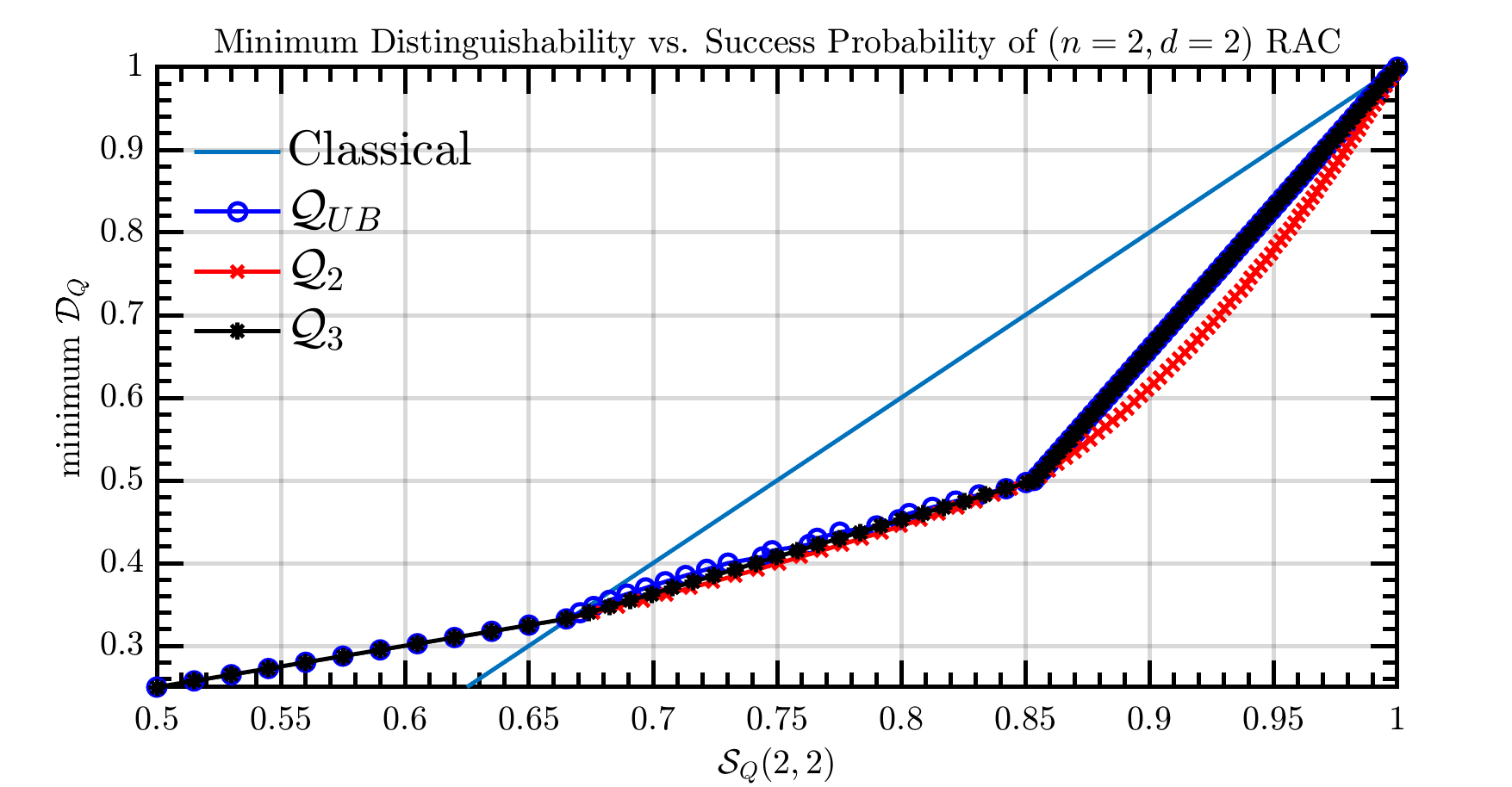
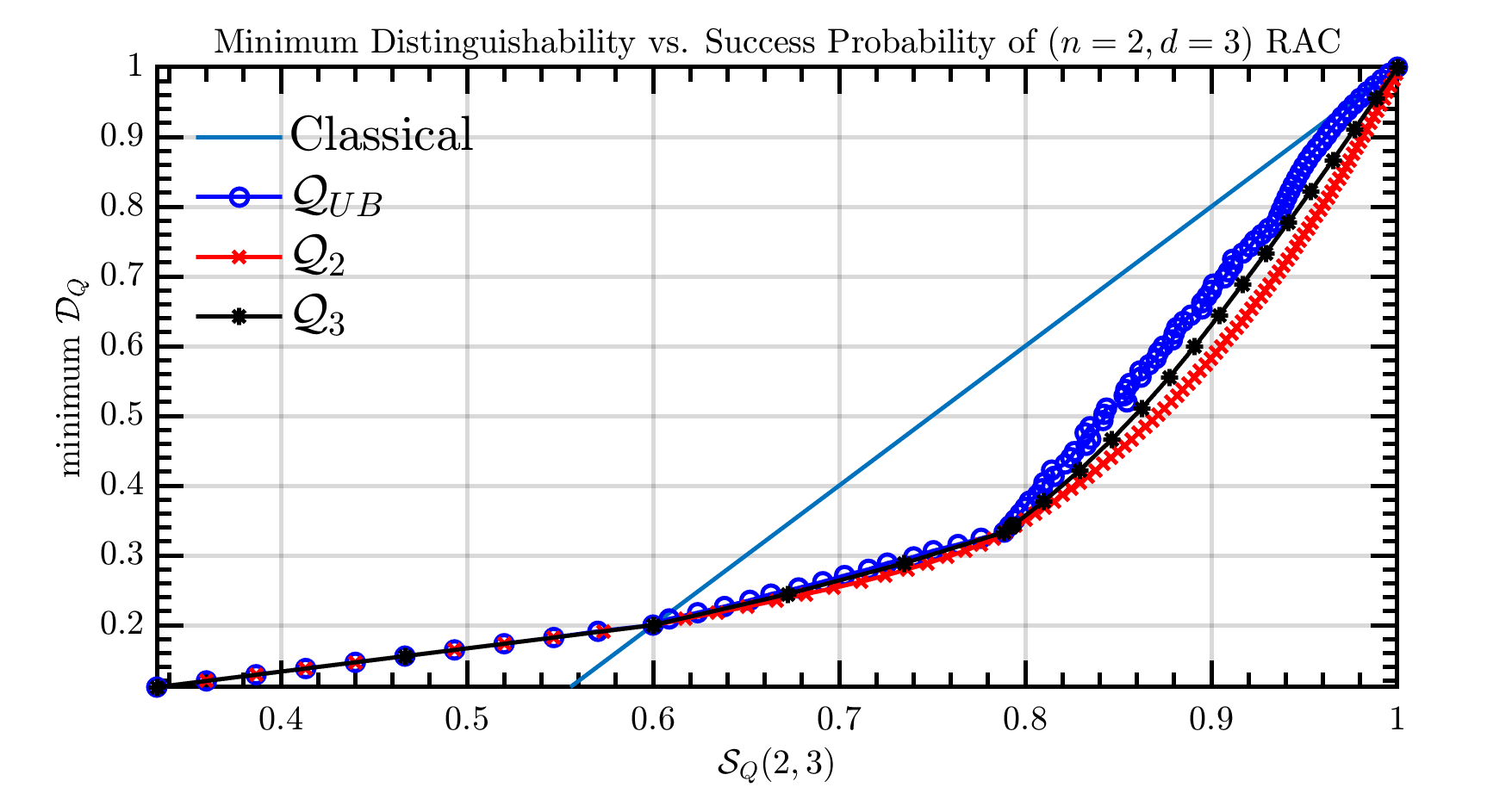
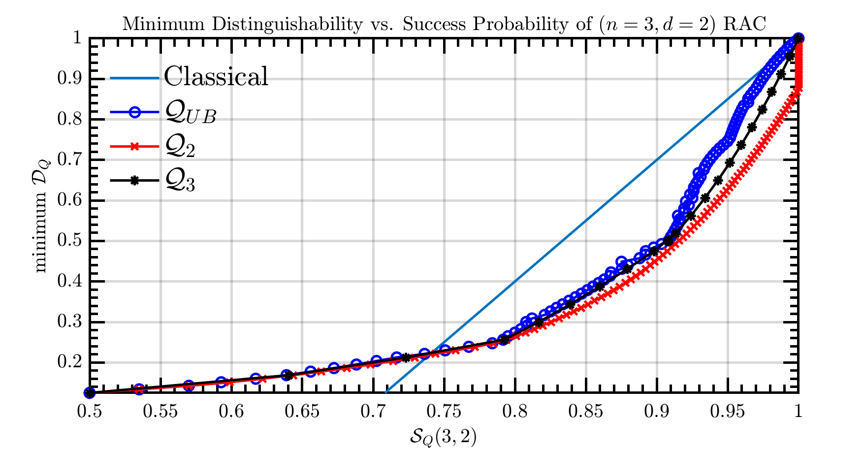
Figure 1: Distinguishability in classical and quantum communication vs. the average success probability is presented for three different RACs. The lower bound on $\mathcal{D}_{C}$ from Eq. (16) is labelled as ’Classical’. By varying values of the success probability $\mathcal{S}(n,d)$, the upper bound on the minimum $\mathcal{D}_{Q}$ is determined by implementing the see-saw method of semi-definite programming Chaturvedi et al. (2021). Referred to as $\mathcal{Q}_{UB}$, this bound is obtained for $d^{n}$-dimensional quantum systems and is certainly achievable in quantum theory. The other two bounds are derived through the semi-definite hierarchy introduced in Tavakoli et al. (2022); Chaturvedi et al. (2021) up to the 2nd and 3rd levels, denoted as $\mathcal{Q}_{2}$ and $\mathcal{Q}_{3}$. These lower bounds on minimum $\mathcal{D}_{Q}$ are valid for arbitrary dimensional quantum states. The quantum advantage is present whenever $\mathcal{Q}_{UB}$ falls below the classical lower bound. For some values of $\mathcal{S}(n,d)$, the classical values are less than $\mathcal{Q}_{UB}$ in the plots, as Eq. (16) provides a lower bound on $\mathcal{D}_{C}$ that is not tight.

Theorem 2.

There exist quantum strategies in random access codes for $n=2$ such that

$$\frac{\mathcal{D}^{\mathcal{S}}_{C}}{\mathcal{D}^{\mathcal{S}}_{Q}}\geqslant\sqrt{d},\ \text{ where }\ \mathcal{S}(2,d)=\frac{1}{2}\left(1+\frac{1}{\sqrt{d}}\right).$$ (28)

Proof.

There exists a known quantum strategy involving $d$-dimensional quantum states and measurements for the case of $n=2$ and arbitrary $d$. This strategy achieves $\mathcal{S_{Q}}(2,d)=1/2\left(1+1/\sqrt{d}\right)$ by employing measurements performed by Bob in two mutually unbiased bases in $\mathbbm{C}^{d}$ Aguilar et al. (2018). According to (11), this quantum strategy must adhere to the constraint $\mathcal{D}_{Q}\leqslant 1/d$. Conversely, if we set $n=2$ and $\mathcal{S}_{C}=1/2\left(1+1/\sqrt{d}\right)$ in (16), we deduce that $1/\sqrt{d}\leqslant\mathcal{D}_{C}$. Consequently, (28) holds.     $\sqcap$$\sqcup$

IV Equality problem defined by graphs

The communication task is defined by an arbitrary graph $G$ having $N$ vertices. Alice and Bob receive input from the vertex set of $G$, i.e., $x,y\in[N]$, sampled from the uniform distribution. Let $G_{x}$ denote the set of vertices in $G$ that are adjacent to $x$, with $N_{x}$ representing the number of vertices adjacent to $x$. In the task, there is a promise that $x=y$ or $x\in G_{y}$. Bob’s aim is to differentiate between these two cases, giving the correct output $z=1$ if $x=y$ and $z=2$ if $x\in G_{y}$. Hence, the success metric,

$$\mathcal{S}(G)=\frac{1}{\sum_{x}N_{x}+N}\sum_{y=1}^{N}\left(p(1|x=y,y)+\sum_{x\in G_{y}}p(2|x,y)\right).$$ (29)

The quantum advantage for this task in terms of the dimension of the communicated systems has been studied in Saha and Chaturvedi (2019); Gupta et al. (2023). Concerning the distinguishability of the sender’s input, we have the following result.

Theorem 3.

For any graph $G$, the following holds in classical communication,

$$\frac{(\sum_{x}N_{x}+N)(\mathcal{S}_{C}(G)-1)+N}{N\alpha(G)}\leqslant\mathcal{D}_{C},$$ (30)

where $\alpha(G)$ is the independence number of the graph $G$.

Proof.

First, we express the average success metric (29) in terms of its general form (1) by defining

$$c(x,y,z)=\frac{1}{(\sum_{x}N_{x}+N)}\times\begin{cases}1,&\text{if $z=1,x=y$}\\ 1,&\text{if $z=2,x\in G_{y}$}\\ $0$,&\text{otherwise.}\end{cases}$$ (31)

Substituting these values of $c(x,y,z)$ into (8), we obtain

$$\mathcal{S}_{C}(G) = 1-\min_{p_{e}(m|x)}\frac{1}{\sum_{x}N_{x}+N}\times$$

$$\sum_{m}\Bigg{[}\underbrace{\sum^{N}_{y=1}\min\Bigg{\{}p_{e}(m|x=y),\sum_{x\in G_{y}}p_{e}(m|x)\Bigg{\}}}_{\chi(m)}\Bigg{]}.$$

The underlined term in (IV) is denoted by $\chi(m)$. The distinguishability of input variable $x$ in this task is given by,

$$\mathcal{D}_{C}=\frac{1}{N}\sum_{m}\max_{x}\bigg{\{}p_{e}(m|x)\bigg{\}}.$$ (33)

For this proof, our primary goal is to show

$$\chi(m)+\alpha(G)\max_{x}p_{e}(m|x)\geqslant\sum_{x}p_{e}(m|x),\ \ \forall m.$$ (34)

Let us fix a value of $m$. For any given encoding $\{p_{e}(m|x)\}$, consider the set $T\subseteq[N]$ such that

$$\min\Bigg{\{}p_{e}(m|y),\sum_{x\in G_{y}}p_{e}(m|x)\Bigg{\}}=\sum_{x\in G_{y}}p_{e}(m|x),\ \forall y\in T.$$ (35)

Subsequently, we can write

$$\chi(m)=\sum_{y\notin T}p_{e}(m|y)+\sum_{y\in T}\left(\sum_{x\in G_{y}}p_{e}(m|x)\right).$$ (36)

Further, we divide the set $T$ into two partitions: first, $T_{I}$ containing the vertices that do not share any common edge, and second, $T\setminus T_{I}$. Note that the subset $T_{I}$ must be an independent set of the induced subgraph made of all the vertices belonging to $T$. For every $y\in T\setminus T_{I},$ there exists another $y^{\prime}\in T\setminus T_{I}$ such that $y\in G_{y^{\prime}}$. This observation allows us to express (36) as

$$\chi(m) \geqslant \sum_{y\notin T}p_{e}(m|y)+\sum_{y\in T\setminus T_{I}}p_{e}(m|y)$$ (37)

$$+\sum_{y\in T_{I}}\left(\sum_{x\in G_{y}}p_{e}(m|x)\right)$$

$$\geqslant \sum_{y\notin T}p_{e}(m|y)+\sum_{y\in T\setminus T_{I}}p_{e}(m|y).$$

Adding $\sum_{y\in T_{I}}p_{e}(m|y)$ on both sides of the above equation, we get

$$\chi(m)+\sum_{y\in T_{I}}p_{e}(m|y)\geqslant\sum_{y=1}^{N}p_{e}(m|y).$$ (38)

For any given set $T$, the cardinality of the subset $T_{I}$ is, at most, $\alpha(G)$, the independence number of $G$. This implies

$$\alpha(G)\max_{y}p_{e}(m|y)\geqslant\sum_{y\in[T_{I}]}p_{e}(m|y).$$ (39)

By substituting the above upper bound in (38), we recover (34). Subsequently, summing over $m$ on both sides of (34) results

$$\sum_{m}\chi(m)+\alpha(G)\sum_{m}\max_{x}p_{e}(m|x)\geqslant\sum_{m}\sum_{x}p_{e}(m|x),$$ (40)

which, due to (33), reduces to

$$\sum_{m}\chi(m)\geqslant N(1-\alpha(G)\mathcal{D}_{C}).$$ (41)

Finally, by replacing the above upper bound on $\sum_{m}\chi(m)$ into (IV) we get

$$\mathcal{S}_{C}(G)\leqslant 1-\frac{N(1-\alpha(G)\mathcal{D}_{C})}{\sum_{x}N_{x}+N},$$ (42)

which, after some rearrangements, becomes (30).     $\sqcap$$\sqcup$

An important inquiry is to identify the simplest graph where quantum methods exhibit an advantage over classical ones. Based on the classical constraint given by (30), we observe that any graph with vertices up to 4 will have no quantum advantage. In order to show there is no quantum advantage, it is sufficient to consider non-isomorphic graphs. Among connected graphs with four vertices, there are six non-isomorphic graphs, and there are two non-isomorphic connected graphs with three vertices (illustrated below).

For each of these eight graphs, we execute semi-definite optimization, based on the method proposed in Chaturvedi et al. (2021); Tavakoli et al. (2022), to obtain an upper bound on the value of $(\mathcal{D}_{C}-\mathcal{D}_{Q})$ for all possible values of $\mathcal{S}(G)$. This optimization yields the value of zero, which reveals that there is no advantage for any of these graphs, irrespective of the values of $\mathcal{S}(G)$. We will now show that the communication task defined by a graph with five vertices does exhibit quantum advantages.

Before delving into this, let us consider a form of quantum strategy for the equality problem given a graph $G$. The strategy is defined by a set of $N$ quantum states $\{|\psi_{x}\rangle\}_{x=1}^{N}\in\mathbbm{C}^{d},$ with

$$\rho_{x}=|\psi_{x}\rangle\!\langle\psi_{x}|,\ M_{1|y}=|\psi_{y}\rangle\!\langle\psi_{y}|,\ M_{2|y}=\mathbbm{1}-|\psi_{y}\rangle\!\langle\psi_{y}|,$$ (43)

where $\rho_{x}$ is the quantum state sent by Alice for input $x$, and the binary outcome measurements performed by Bob on the received quantum state for input $y$ are expressed as $\{M_{1|y},M_{2|y}\}$. For this strategy, a straightforward calculation leads to

$$\mathcal{S}_{Q}(G)=1-\frac{1}{\sum_{x}N_{x}+N}\sum_{y}\sum_{x\in G_{y}}|\langle\psi_{x}|\psi_{y}\rangle|^{2}.$$ (44)

Simultaneously, it holds that $\mathcal{D}_{Q}\leqslant d/N$.

Theorem 4.

Let us consider $N$-cyclic graph (denoted by $\Delta_{N}$) such that $N\geqslant 5$ and odd. There exist quantum strategies with 2-dimensional systems such that

$$\frac{\mathcal{D}^{\mathcal{S}}_{C}(\Delta_{N})}{\mathcal{D}^{\mathcal{S}}_{Q}(\Delta_{N})}=\frac{N}{N-1}\left({1-2\sin^{2}\left(\frac{\pi}{2N}\right)}\right)>1,$$ (45)

for $\mathcal{S}=1-\frac{2}{3}\sin^{2}\big{(}\frac{\pi}{2N}\big{)}$.

Proof.

Let us consider a quantum strategy given by (43) where the states $\{|\psi_{x}\rangle\}_{x}\in\mathbbm{C}^{2}$ are given by

$$|\psi_{x}\rangle=\cos\left(\frac{(x-1)\beta}{2}\right)|0\rangle+\sin\left(\frac{(x-1)\beta}{2}\right)|1\rangle,$$ (46)

and $\beta=\big{(}\frac{(N-1)\pi}{N}\big{)}$. These states form a regular $N$-gon in the $X$-$Z$ plane of the Bloch sphere such that the angle between the Bloch vectors of $|\psi_{x}\rangle$ and $|\psi_{x\pm 1}\rangle$ is $\beta$. The Bloch vectors of these states for $N=5$ and $N=7$ are shown below.

For this quantum strategy, $|\langle\psi_{x}|\psi_{y}\rangle|=\sin\big{(}\frac{\pi}{2N}\big{)}$ for any pair of $x,y,$ that are connected by an edge. By substituting the expression in (44) and $N_{x}=2,\forall x$, we obtain

$$\mathcal{S}_{Q}(\Delta_{N})=1-\frac{2}{3}\sin^{2}\Big{(}\frac{\pi}{2N}\Big{)}.$$ (47)

Replacing this value of $\mathcal{S}_{Q}$ in (30) with $\alpha(\Delta_{N})=(N-1)/2$ and other specifications of $N$-cyclic graph, we get

$$\mathcal{D}^{\mathcal{S}}_{C}(\Delta_{N})\geqslant\frac{2}{N-1}\Big{(}1-2\sin^{2}\frac{\pi}{2N}\Big{)}.$$ (48)

From the fact that $\mathcal{D}^{\mathcal{S}}_{Q}(\Delta_{N})\leqslant 2/N$ and the above relation (48), we obtain (45). Fig. 2 depicts how the ratio (45) changes with $N$.     $\sqcap$$\sqcup$

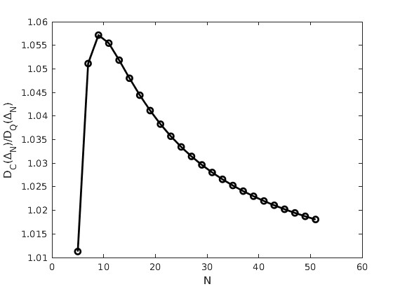
Figure 2: The ratio between classical and quantum distinguishability of input states as a function of $N$ for the communication tasks defined by regular $N$-cyclic graph, where $\mathcal{S}=1-(2/3)\sin^{2}(\pi/2N)$. Here, $N\geqslant 5$ and odd. The ratio reduces to $1$ as $N\rightarrow{\infty}$.

Consider the set of vectors in $\mathbbm{C}^{d}$ of the form

$$|\psi_{x}\rangle=(1/\sqrt{d})\left[(-1)^{x_{1}},(-1)^{x_{2}},\ldots,(-1)^{x_{d}}\right]^{T},$$ (49)

where every $x_{i}\in\{0,1\}$. This set comprises $2^{d}$ distinct vectors, and two vectors are orthogonal when the values of $x_{i}$ differ in exactly $d/2$ places. The orthogonality relations among these vectors can be represented through a graph, commonly known as the Hadamard graph $(H_{d})$, where the vertices symbolize the vectors, and two vertices are connected by an edge if the respective vectors are orthogonal. Consequently, one can consider the communication task based on $H_{d}$, previously introduced as the distributed Deutsch-Jozsa task Buhrman et al. (2010). Hereafter, we demonstrate that the ratio $\mathcal{D}^{\mathcal{S}}_{C}/\mathcal{D}^{\mathcal{S}}_{Q}$ experiences exponential growth with $d$.

Theorem 5.

For the Hadamard graph $H_{d}$ where $d$ is divisible by 4,

$$\frac{\mathcal{D}^{\mathcal{S}}_{C}}{\mathcal{D}^{\mathcal{S}}_{Q}}\geqslant\frac{(1.005)^{d}}{d},\text{ where }\mathcal{S}=1.$$ (50)

Proof.

Clearly, the quantum strategy of the form (43) such that $|\psi_{x}\rangle$ given by (49), perfectly accomplishes the task, leading to $\mathcal{S}(H_{d})=1$. Additionally, in this strategy, as per (1), $\mathcal{D}_{Q}\leqslant d/2^{d}$. On the classical side, according to (30), we know that $\mathcal{S}_{C}(H_{d})=1$ only if $\mathcal{D}_{C}=1/\alpha(H_{d})$. The result established by Frankl-Rödl Frankl and Rodl (1987) implies that $\alpha(H_{d})\leqslant 1.99^{d}$, specifically when $d$ is divisible by $4$ (refer to Theorem 1.11 in Frankl and Rodl (1987)). As a consequence, we have (50).     $\sqcap$$\sqcup$

Theorem 6.

For any graph $G$, say $\beta(G)$ is the minimum dimension $d$ such that there exists $N$ number of quantum states $\{|\psi_{x}\rangle\}_{x=1}^{N}\in\mathbbm{C}^{d}$ satisfying the orthogonality relations according to $G$, that is, $\langle\psi_{x}|\psi_{y}\rangle=0$ for every pair of vertices $x,y,$ that are connected in $G$. Then,

$$\frac{\mathcal{D}^{\mathcal{S}}_{C}}{\mathcal{D}^{\mathcal{S}}_{Q}}\geqslant\frac{N}{\alpha(G)\beta(G)},\ \ \text{ for }\mathcal{S}=1.$$ (51)

Proof.

If there exist states $\{|\psi_{x}\rangle\}_{x}\in\mathbbm{C}^{d}$ that fulfill the orthogonality conditions according to $G$, then the quantum strategy given by (43) achieves $\mathcal{S}(G)=1$, with $\mathcal{D}_{Q}\leqslant d/N$. Conversely, according to (30), for $\mathcal{S}_{C}(G)=1$, it follows that $\mathcal{D}_{C}\geqslant 1/\alpha(G)$. Combining these two observations yields (51).     $\sqcap$$\sqcup$

The aforementioned result suggests that a graph offers quantum advantages for achieving the respective tasks perfectly ($\mathcal{S}=1$) if

$$\frac{N}{\alpha(G)\beta(G)}>1.$$ (52)

Interestingly, a graph exhibits state-independent contextuality if and only if its fractional chromatic number, denoted as $\chi_{f}(G)$, is greater than $\beta(G)$, that is, $\chi_{f}(G)>\beta(G)$ Ramanathan and Horodecki (2014). Additionally, for any graph, $\chi_{f}(G)\geqslant N/\alpha(G)$. Consequently, any graph satisfies the condition (52) meets the state-independent contextuality criterion. It is important to note that the converse is not universally true. However, for vertex-transitive graphs, the reverse implication does hold, as these graphs adhere to the equality $\chi_{f}(G)=N/\alpha(G)$. Notably, the smallest graph meeting the condition (52) was identified as the Yu-Oh graph, comprising 13 vertices Cabello et al. (2015).

V Pair distinguishability task

We consider a generalized version of the task introduced in Chaturvedi and Saha (2020). Alice receives input $x\in[N]$ with $p_{x}=1/N$ and Bob receives a pair of inputs $y\equiv(x,x^{\prime})$ randomly such that $x,x^{\prime}\in\{1,\cdots,N\}$ and $x<x^{\prime}$. The task is to guess $x$. In other words, given Bob’s input $(x,x^{\prime})$, the task is to distinguish between these two inputs. Subsequently, the average success metric,

$$\mathcal{S}(N)=\frac{1}{N(N-1)}\sum_{\begin{subarray}{c}x,x^{\prime}\\ x<x^{\prime}\end{subarray}}\big{[}p(x|x,(x,x^{\prime}))+p(x^{\prime}|x^{\prime},(x,x^{\prime}))\big{]}.$$ (53)

Theorem 7.

The following hold for classical communication,

$$(N-1)(\mathcal{S}_{C}(N)-1)+1\leqslant\mathcal{D}_{C}.$$ (54)

Proof.

For this task, the form of success metric (8) reduces to

$$\mathcal{S}_{C}(N) = 1-\min_{\{p_{e}(m|x)\}}\frac{1}{N(N-1)}\times$$ (55)

$$\sum_{m}\sum_{\begin{subarray}{c}x,x^{\prime}\\ x<x^{\prime}\end{subarray}}\min\left\{p_{e}(m|x),p_{e}(m|x^{\prime})\right\},$$

after substituting the following expression

$$c(x,(x,x^{\prime}),z)=\frac{1}{N(N-1)}\times\begin{cases}1,&\text{if $z=x,$ $x\in\{x,x^{\prime}\}$}\\ $0$,&\text{otherwise.}\end{cases}$$ (56)

We use the fact that any set of non-negative numbers $\{a_{i}\}$ with $i=1,\cdots,N$, satisfies the relation

$$\sum_{i<j}\min\{a_{i},a_{j}\}\geqslant\sum_{i}a_{i}-\max\{a_{1},\cdots,a_{N}\}.$$ (57)

Replacing $a_{x}$ by $p_{e}(m|x)$ into the above relation, we get

$$\sum_{x<x^{\prime}}\min\{p_{e}(m|x),p_{e}(m|x^{\prime})\}$$ (58)

$$\geqslant \sum_{x}p_{e}(m|x)-\max_{x}\{p_{e}(m|x)\}.$$

Next, we take summation over $m$ on both sides and replace the expression of distinguishability (6) to obtain

$$\sum_{m}\sum_{x<x^{\prime}}\min\{p_{e}(m|x),p_{e}(m|x^{\prime})\}\geqslant N(1-\mathcal{D}_{C}).$$ (59)

The left-hand side of the above inequality appears on the right-hand side of (55). Hence, by substituting the lower bound from (59) into (55), we deduce (54).     $\sqcap$$\sqcup$

Let us discuss a few quantum strategies for this task that provide advantages. One interesting feature of this task is the fact that $\mathcal{S}_{Q}$ is fixed by the set of quantum state $\{\rho_{x}\}$ communicated by Alice. Specifically, due to the Helstrom norm Helstrom (1976),

$$\mathcal{S}_{Q}=\frac{1}{2}+\frac{1}{2N(N-1)}\sum_{\begin{subarray}{c}x,x^{\prime}\\ x<x^{\prime}\end{subarray}}\|\rho_{x}-\rho_{x^{\prime}}\|.$$ (60)

Consider the following $N=d+1$ states in $\mathbbm{C}^{d}$ Brunner et al. (2013),

$$|\psi_{x}\rangle=\frac{1}{\sqrt{d}}\sum_{k=0}^{d-1}e^{\frac{i2\pi kx}{N}}|k\rangle,$$ (61)

where $x\in[d+1]$. We evaluate $\mathcal{S}$ from (60) for these states and further obtain the corresponding $\mathcal{D}_{C}$ from (54), which are given as follows:

$N$	$\mathcal{S}$	$\mathcal{D}_{C}$	$\mathcal{D}_{Q}$
3	0.933	0.866	$~{}~{}\leqslant 0.667$

Similarly, invoking the qubit states $|\psi_{x}\rangle=\cos{\frac{x\pi}{N}}|0\rangle+\sin{\frac{x\pi}{N}}|1\rangle$, where $x\in[N]$, we obtain the following values.

$N$	$\mathcal{S}$	$\mathcal{D}_{C}$	$\mathcal{D}_{Q}$
3	0.933	0.866	$~{}~{}\leqslant 0.667$
4	0.9	0.7	$~{}~{}\leqslant 0.5$
5	0.8847	0.5388	$~{}~{}\leqslant 0.4$
6	0.8732	0.366	$~{}~{}\leqslant 0.333$

VI Conclusions

Communication complexity plays a crucial role in information science, and quantum theory offers a notable advantage over classical methods. Traditionally, one-way communication complexity is quantified by the minimal dimension of systems that the sender uses to achieve a given task. However, in this investigation, we take a fresh approach by evaluating communication complexity based on the distinguishability of the sender’s input, without imposing constraints on the dimension of the communicated systems. This perspective gains significance when preserving the confidentiality of the sender’s input is paramount. Moreover, the dimension independence nature of this measure implies that quantum advantage signifies something unattainable in classical communication and does not rely on specific details of the physical system.

We concentrate on two significant categories of communication complexity tasks: the general version of random access codes and equality problems defined by graphs. Lower bounds on the distinguishability of the sender’s input are derived as a function of the success metric for these tasks in classical communication. Remarkably, we demonstrate that the ratio between classical and quantum distinguishability increases with the complexity of these tasks, reaching arbitrarily large values.

For the RACs considered in Fig. 1, the best success probabilities using $d$-dimension classical systems are 3/4, 3/4 and 2/3, respectively. On the other hand, we find quantum advantages (Fig. 1) even when the success probabilities are less than these values. Therefore, our study of RACs reveals instances where quantum advantage in dimension is absent, but the quantum advantage in distinguishability exists. Notably, for $(d,n=2)$ RAC, we obtain an unbounded advantage, which does not occur with dimension. Instances of quantum advantage in dimension but no quantum advantage in distinguishability remain unknown. Other future works could explore advantageous quantum protocols for random access codes with higher $n$ and for equality problems based on different graphs. Additionally, proposing privacy-preserving computational schemes based on these results and exploring other communication complexity tasks with practical applications are avenues for further research.

Acknowledgements

AC acknowledges financial support by NCN grant SONATINA 6 (contract No. UMO-2022/44/C/ST2/00081).

References

- Kushilevitz and Nisan (2006) E. Kushilevitz and N. Nisan, Communication Complexity (Cambridge Univ Press, Cambridge, UK, 2006).
- Roughgarden (2016) T. Roughgarden, Communication Complexity (for Algorithm Designers), Foundations and Trends® in Theoretical Computer Science 11, 217 (2016).
- Rao and Yehudayoff (2020) A. Rao and A. Yehudayoff, Communication Complexity: and Applications (Cambridge University Press, 2020).
- Yao (1979) A. C.-C. Yao (Association for Computing Machinery, New York, NY, USA, 1979).
- (5) R. Raz, Proceedings of the 31st Annual ACM Symposium on Theory of Computing (ACM, New York, 1999).
- Buhrman et al. (2010) H. Buhrman, R. Cleve, S. Massar, and R. de Wolf, Rev. Mod. Phys. 82, 665 (2010).
- Buhrman et al. (2001) H. Buhrman, R. Cleve, J. Watrous, and R. de Wolf, Phys. Rev. Lett. 87, 167902 (2001).
- Buhrman et al. (1998) H. Buhrman, R. Cleve, and A. Wigderson, in Proceedings of the Thirtieth Annual ACM Symposium on Theory of Computing (1998) p. 63.
- de Wolf (2002) R. de Wolf, Theor. Comput. Sci. 287, 337 (2002).
- Buhrman et al. (2016) H. Buhrman, Łukasz Czekaj, A. Grudka, M. Horodecki, P. Horodecki, M. Markiewicz, F. Speelman, and S. Strelchuk, Proceedings of the National Academy of Sciences 113, 3191 (2016).
- Saha and Chaturvedi (2019) D. Saha and A. Chaturvedi, Phys. Rev. A 100, 022108 (2019).
- Gupta et al. (2023) S. Gupta, D. Saha, Z.-P. Xu, A. Cabello, and A. S. Majumdar, Phys. Rev. Lett. 130, 080802 (2023).
- Ekert (1991) A. K. Ekert, Phys. Rev. Lett. 67, 661 (1991).
- Gisin et al. (2002) N. Gisin, G. Ribordy, W. Tittel, and H. Zbinden, Rev. Mod. Phys. 74, 145 (2002).
- Casaccino et al. (2008) A. Casaccino, E. F. Galvão, and S. Severini, Phys. Rev. A 78, 022310 (2008).
- Czechlewski et al. (2018) M. Czechlewski, D. Saha, A. Tavakoli, and M. Pawłowski, Phys. Rev. A 98, 062305 (2018).
- Frankl and Rodl (1987) P. Frankl and V. Rodl, Trans. Am. Math. Soc. 300, 259 (1987).
- Chaturvedi and Saha (2020) A. Chaturvedi and D. Saha, Quantum 4, 345 (2020).
- Tavakoli et al. (2022) A. Tavakoli, E. Zambrini Cruzeiro, E. Woodhead, and S. Pironio, Quantum 6, 620 (2022).
- Chaturvedi et al. (2021) A. Chaturvedi, M. Farkas, and V. J. Wright, Quantum 5, 484 (2021).
- Aguilar et al. (2018) E. A. Aguilar, J. J. Borkała, P. Mironowicz, and M. Pawłowski, Phys. Rev. Lett. 121, 050501 (2018).
- Ramanathan and Horodecki (2014) R. Ramanathan and P. Horodecki, Phys. Rev. Lett. 112, 040404 (2014).
- Cabello et al. (2015) A. Cabello, M. Kleinmann, and C. Budroni, Phys. Rev. Lett. 114, 250402 (2015).
- Helstrom (1976) C. W. Helstrom, Quantum Detection and Estimation Theory (Academic, New York, 1976).
- Brunner et al. (2013) N. Brunner, M. Navascués, and T. Vértesi, Phys. Rev. Lett. 110, 150501 (2013).