Fully dynamic $G3W2$ self-energy for finite systems: Formulas and benchmark

Abstract

Over the years, Hedin’s $GW$ self-energy has been proven to be a rather accurate and simple approximation to evaluate electronic quasiparticle energies in solids and in molecules. Attempts to improve over the simple $GW$ approximation, the so-called vertex corrections, have been constantly proposed in the literature. Here, we derive, analyze, and benchmark the complete second-order term in the screened Coulomb interaction $W$ for finite systems. This self-energy named $G3W2$ contains all the possible time orderings that combine 3 Green’s functions $G$ and 2 dynamic $W$. We present the analytic formula and its imaginary frequency counterpart, the latter allowing us to treat larger molecules. The accuracy of the $G3W2$ self-energy is evaluated on well-established benchmarks (GW100, Acceptor 24 and Core 65) for valence and core quasiparticle energies. Its link with the simpler static approximation, named SOSEX for static screened second-order exchange, is analyzed, which leads us to propose a more consistent approximation named 2SOSEX. In the end, we find that neither the $G3W2$ self-energy nor any of the investigated approximations to it improve over one-shot $G_{0}W_{0}$ with a good starting point. Only quasi-particle self-consistent $GW$ HOMO energies are slightly improved by addition of the $G3W2$ self-energy correction. We show that this is due to the self-consistent update of the screened Coulomb interaction leading to an overall sign change of the vertex correction to the frontier quasiparticle energies.

1 Introduction

Hedin’s $GW$ approximation ¹ has become a wide-spread method to evaluate the electronic quasiparticle energies ^{2, 3}. While first introduced for extended systems ^{1, 4, 5, 6, 7}, it has recently permeated to molecular systems ^{8, 9, 10, 11, 12, 13, 14, 15, 16, 17, 18, 19, 20, 21, 22, 23, 24, 25, 26, 27, 28, 29, 30, 31, 32}, and even more recently to the core state binding energy ^{33, 34, 35}. The success of the $GW$ approximation owes much to its cost-effectiveness: $GW$ is both rather simple and reasonably accurate.

However, almost as old as $GW$ itself, there have been attempts to go beyond the mere $GW$ self-energy. In the framework of the many-body equations as formulated by Hedin ^{1, 36}, these corrections are coined “vertex correction”, since they necessarily involve the complicated 3-point vertex function $\tilde{\Gamma}$. The vertex corrections appear in two distinct locations in the equations, firstly as a correction to the polarizability and secondly as a correction to the self-energy itself. The first kind of vertex corrections are less computationally demanding and have been tried first ^{37, 8, 38, 39}. But a recent work ⁴⁰ indicates the vertex corrections in the polarizability systematically only have a mild effect, even though there exists a series of studies that include both vertices at once. ^{41, 42, 43, 44}

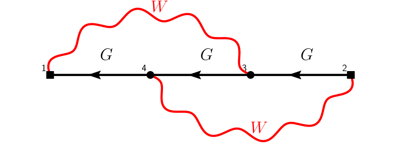
Figure 1: Dynamical $G3W2$ Goldstone-Feynman diagram. Red wiggly lines represent the screened Coulomb interactions $W$, straight black lines with an arrow the Green’s functions $G$. Entry and exit points of the self-energy are marked with a square.

Here, we focus on the latter type of vertex corrections: those that modify the electronic self-energy itself. The polarizability is kept at the simple random-phase approximation level. Quite the opposite, for the self-energy the intrinsic 3-point nature of the vertex function cannot be avoided and the practical derivations and calculations have to cope with this additional complexity. Here we focus in particular on the second-order diagram that we name $G3W2$ following Kutepov ⁴⁵ and whose Feynman-Goldstone representation is given in Figure 1. Gradual progress has been made towards the complete inclusion of the second-order term. Most of the complexity arises from the screened Coulomb interaction $W(\omega)$ that is a dynamic quantity as opposed to the bare Coulomb interaction $v$. Earlier simpler approximations such as the second-order exchange (SOX) and the second-order screened exchange (SOSEX) exist. SOX is obtained when the two $W$ are replaced by $v$. This approximation has been known for long ⁴⁶ but its performance is very poor ^{15, 47}. The next step, SOSEX, consists of one dynamic $W(\omega)$ and one static $v$ ⁴⁸. SOSEX performance is somewhat better than SOX ⁴⁷. The complete calculation of the dynamic $G3W2$ term has been recently claimed by Wang, Rinke, and Ren ⁴⁹. Note that statically screened approximations to $G3W2$ using $W(\omega=0)$ instead of the dynamic $W(\omega)$ have also been proposed in the literature ⁵⁰ with interesting performance.^{51, 52} There are clues from the homogeneous electron gas model that the $G3W2$ diagram contains undesired features for extended systems ^{53, 54}. However an evaluation for molecular systems is missing as of today.

In this article, we concentrate on the fully dynamic $G3W2$ self-energy. We derive its analytic formula as well as its complex frequency numerical quadrature. Our expressions depart from the one reported in Ref. 49. A double frequency integral has to be performed in our equations, which makes the practical calculations very challenging. We analyze the different contributions to the $G3W2$ self-energy induced by the possible different time-orderings. Consistent numerical results are obtained with different expressions and two independent codes, MOLGW ⁵⁵ and BAND.^{56, 57} Thanks to our analytic expressions for both $G3W2$ and SOSEX, we are able to accurately evaluate them for the core states. We then test the performance of $G3W2$ and its approximations (SOX, SOSEX) on well-established benchmarks (GW100 ²⁰, Acceptor24⁵⁸, and a subset of CORE65³⁵).

2 $G3W2$ self-energy derivation

2.1 $G3W2$ self-energy obtained from Hedin’s equations

There are many equivalent ways to obtain the analytic expression of the self-energy diagram drawn in Fig. 1. We follow here the functional path as exposed by Hedin in his seminal paper¹. More specifically, we closely stick to Strinati’s review notations⁵⁹, except for the exchange-correlation self-energy that we denote $\Sigma$ instead of $M$.

The exact electronic self-energy $\Sigma$ reads

$$\Sigma(1,2)=\mathrm{i}\int d3d4G(1,4)W(1^{+},3)\tilde{\Gamma}(4,2;3),$$ (1)

where the numbers, such as 1, conventionally represent a combined index over space and time ($\mathbf{r}_{1}$,$t_{1}$). $G$ is the time-ordered Green’s function, $W$ is the dynamically screened Coulomb interaction, and $\tilde{\Gamma}(4,2;3)$ is the irreducible 3-point vertex function. These three functions have been already mentioned in the introduction. According to Strinati ⁵⁹, the irreducible vertex has a closed expression:

$$\tilde{\Gamma}(4,2;3)=\delta(4,2)\delta(4,3)+\int d5678\frac{\delta\Sigma(4,2)}{\delta G(5,6)}G(5,7)G(8,6)\tilde{\Gamma}(7,8;3).$$ (2)

Obviously, Eq. (2) is tremendously complex involving 3- and 4-point functions. The usual $GW$ approximation is obtained when Eq. (2) is truncated to the mere $\delta$-functions (first term in the right-hand side). This approximation introduced in Eq. (1) indeed yields

$$\Sigma(1,2)=\mathrm{i}G(1,2)W(1^{+},2).$$ (3)

Let us approximate $\tilde{\Gamma}(4,2;3)$ in a slightly more sophisticated way. In Eq. (2), consider that the irreducible vertex in the right-hand side is simply

$$\tilde{\Gamma}(7,8;3)\approx\delta(7,8)\delta(7,3).$$ (4a)

In addition, use the $$GW \Sigma G$$ self-energy in the derivative of with respect to in the same Eq. (2), which gives

$$\frac{\delta\Sigma(4,2)}{\delta G(5,6)}\approx\mathrm{i}W(4,2)\delta(4,5)\delta(2,6),$$ (4b)

which amounts to neglecting the derivative of $$W G$$ with respect to .

With these two simplifications, Eq. (2) reduces to

$$\tilde{\Gamma}(4,2;3)\approx\delta(4,2)\delta(4,3)+\mathrm{i}W(4,2)G(4,3)G(3,2),$$ (5)

which is a lot less complex than the original expression.

Plugging Eq. (5) into the expression of the exact self-energy reported in Eq. (1), we obtain our desired expression:

$$\Sigma(1,2)=\mathrm{i}G(1,2)W(1^{+},2)\\ +\mathrm{i}^{2}\int d3d4G(1,4)W(1^{+},3)G(4,3)W(4,2)G(3,2).$$ (6)

The self-energy in Eq. (6) consists of two terms: the usual $GW$ approximation and an additional correction (in other words a “vertex correction”) that we name $G3W2$. The diagrammatic representation of $G3W2$ precisely matches the diagram of Figure 1. Note that the $G3W2$ expression has a double time integral, which still make it quite a challenge for numerical applications.

2.2 $G3W2$, 2SOSEX, SOSEX, and SOX

It is insightful (and convenient for numerics as we will see later) to split the dynamic $G3W2$ self-energy correction into static and dynamic parts thanks to the introduction of the intermediate bare Coulomb interaction $v$.

Dropping the space and time indices for conciseness, one can decompose the $G3W2$ self-energy into 4 terms:

$$\Sigma^{G3W2} = \mathrm{i}^{2}\int GWGWG$$ (7)

$$= \mathrm{i}^{2}\int GvGvG$$

$$+\mathrm{i}^{2}\int G\left[W-v\right]GvG$$

$$+\mathrm{i}^{2}\int GvG\left[W-v\right]G$$

$$+\mathrm{i}^{2}\int G\left[W-v\right]G\left[W-v\right]G.$$

The first term is the well-known SOX term ⁴⁶. The sum of the two first terms form the SOSEX self-energy introduced by Ren and coworkers ⁴⁸.

The second and the third terms are equal since they are completely symmetric through the exchange of integrated indices. We hence propose to name “2SOSEX” the sum of the 3 first terms in Eq. (7). Of course, the last term that contains a genuine time-dependence in both interactions is the most computationally involved.

From the present perspective, there is no specific reason to use SOSEX rather than 2SOSEX. We will study in section 3 the actual performance of each truncation strategy.

2.3 Expression in real frequency domain

For practical implementation and understanding, it is very convenient to work in the frequency domain. As the first terms in Eq. (7) are already known, we now focus on the last, fully-dynamic one.

In the following we introduce $W_{p}$ for the polarizable part of $W$ as

$$W_{p}(1,2)=W(1,2)-v(1,2)\delta(t_{1}-t_{2}).$$ (8)

In many-body perturbation theory at equilibrium, the time-dependencies of $\Sigma$, $G$, and $W$ are only a time differences: e.g. $G(1,2)=G(\mathbf{r}_{1},\mathbf{r}_{2},t_{1}-t_{2})$ ⁴⁶. Omitting space variables for conciseness, the last term in Eq. (7) reads

$$\Sigma^{G3{W_{p}}2}(t_{1}-t_{2})=\mathrm{i}^{2}\int dt_{3}dt_{4}G(t_{1}-t_{4})W_{p}(t_{3}-t_{1})G(t_{4}-t_{3})W_{p}(t_{2}-t_{4})G(t_{3}-t_{2}).$$ (9)

We have used the symmetries $W_{p}(1,3)=W_{p}(3,1)$ and $W_{p}(4,2)=W_{p}(2,4)$ for convenience ⁵⁹.

Then we Fourier-transform of all these functions. The detailed steps that lead to the final expression are given in appendix A. Finally, the fully-dynamic term $\Sigma^{G3{W_{p}}2}$ in the frequency domain reads

$$\Sigma^{G3{W_{p}}2}(\omega)=\left(\frac{\mathrm{i}}{2\pi}\right)^{2}\int d\omega^{\prime}\int d\omega^{\prime\prime}G(\omega+\omega^{\prime})W_{p}(\omega^{\prime})G(\omega+\omega^{\prime}+\omega^{\prime\prime})W_{p}(\omega^{\prime\prime})G(\omega+\omega^{\prime\prime}).$$ (10)

The expression with times had two integrals and it still contains two integrals in the frequency domain.

2.4 Analytic formula

In this section, we derive a fully analytic formula for Eq. (10). This is not only useful for a deeper understanding, but also it is in practice, since some implementations, such as MOLGW ⁵⁵ or Turbomole, ¹⁷ indeed use this strategy.

When starting from a mean-field Kohn-Sham or generalized Kohn-Sham self-consistent solution with (real-valued) eigenstates $\varphi_{p}(\mathbf{r})$ and eigenvalues $\epsilon_{p}$, the corresponding Green’s function $G(\omega)$ reads

$$G(\mathbf{r},\mathbf{r}^{\prime},\omega)=\sum_{i}^{\mathrm{occ}}\frac{\varphi_{i}(\mathbf{r})\varphi_{i}(\mathbf{r}^{\prime})}{\omega-\epsilon_{i}-\mathrm{i}\eta}+\sum_{a}^{\mathrm{virt}}\frac{\varphi_{a}(\mathbf{r})\varphi_{a}(\mathbf{r}^{\prime})}{\omega-\epsilon_{a}+\mathrm{i}\eta}.$$ (11)

We use the usual convention where the indices $a,b,c$ run over virtual molecular orbitals (MO), $i,j,k$ over occupied MO, and $p,q,u,v,w$ over all the MO. $\eta$ symbol stands for a small positive real number that enforces the proper location of the poles in the complex plane: above the real axis for occupied states ($\varepsilon_{i}<\mu$) and below the real axis for virtual states ($\varepsilon_{a}>\mu$). Note that we assume real wavefunctions without loss of generality for finite systems.

The polarizable part of $W$ also can be written analytically provided that the Casida-like equation has been solved for the random-phase approximation ^{60, 17, 55}. $W_{p}(\omega)$ is a sum of pairs of poles $\pm\Omega_{s}$, which account for resonant and antiresonant neutral excitations ⁵⁵:

$$W_{p}(\mathbf{r},\mathbf{r}^{\prime},\omega)=\sum_{s}w_{s}(\mathbf{r})w_{s}(\mathbf{r}^{\prime})\left[\frac{1}{\omega-\Omega_{s}+\mathrm{i}\eta}-\frac{1}{\omega+\Omega_{s}-\mathrm{i}\eta}\right].$$ (12)

Here and in the following the pole index $s$ (and later also $t$) runs over the pairs of poles. Again, the small real positive $\eta$ enforces the correct location of the poles for a time-ordered function. $\Omega_{s}$ are defined as positive energies as obtained from the diagonalization of the Casida-like equation. The resonant excitation count amounts to $N_{o}\times N_{v}$ in a finite basis set, where $N_{o}$ is the number of occupied MO and $N_{v}$ the number of virtual MO.

With these two expressions for the non-interacting $G$ and for $W_{p}$ in Eqs. (11) and (12), there is no obstacle against the complete derivation of $G3W2$ as expressed in Eq. (10). One can apply the complex analysis tools (contour closing and residue theorem) to each of the $2^{5}=32$ cases for occupied or virtual MO in $G$ and resonant or antiresonant poles in $W_{p}$.

Fortunately, 14 terms are strictly zero becase of the poles’ location. The 18 remaining terms have been calculated manually. A calculation for the term involving 3 occupied MO and 2 anti-resonant poles in $W_{p}$ is given as an example in Appendix B.

Introducing $w_{s}^{pq}=\int d\mathbf{r}\varphi_{p}(\mathbf{r})\varphi_{q}(\mathbf{r})w_{s}(\mathbf{r})$, we present the sum of the 18 terms that has been split according to the occupation of the 3 Green’s functions:

$$\Sigma_{pq}^{ooo}(\omega)=\sum_{ts}\sum_{ijk}\frac{w_{t}^{pi}\cdot w_{t}^{jk}\cdot w_{s}^{qk}\cdot w_{s}^{ij}}{(\omega-\epsilon_{i}+\Omega_{t}-2\mathrm{i}\eta)\cdot(\omega-\epsilon_{j}+\Omega_{t}+\Omega_{s}-3\mathrm{i}\eta)\cdot(\omega-\epsilon_{k}+\Omega_{s}-2\mathrm{i}\eta)}$$ (13a)

$$\Sigma_{pq}^{vvv}(\omega)=\sum_{ts}\sum_{abc}\frac{w_{t}^{pa}\cdot w_{t}^{bc}\cdot w_{s}^{qc}\cdot w_{s}^{ab}}{(\omega-\epsilon_{a}-\Omega_{t}+2\mathrm{i}\eta)\cdot(\omega-\epsilon_{b}-\Omega_{t}-\Omega_{s}+3\mathrm{i}\eta)\cdot(\omega-\epsilon_{c}-\Omega_{s}+2\mathrm{i}\eta)}$$ (13b)

$$\Sigma_{pq}^{voo+oov}(\omega)=\sum_{ts}\sum_{ajk}\frac{w_{t}^{pa}\cdot w_{t}^{jk}\cdot w_{s}^{qk}\cdot w_{s}^{aj}}{(\omega-\epsilon_{k}+\Omega_{s}-2\mathrm{i}\eta)\cdot(\Omega_{s}+\epsilon_{a}-\epsilon_{j}-3\mathrm{i}\eta)}\\ \times\left[\frac{2}{\omega-\epsilon_{a}-\Omega_{t}+2\mathrm{i}\eta}-\frac{2}{\omega-\epsilon_{j}+\Omega_{s}+\Omega_{t}-3\mathrm{i}\eta}\right].$$ (13c)

$$\Sigma_{pq}^{ovv+vvo}(\omega)=\sum_{ts}\sum_{ibc}\frac{w_{t}^{pi}\cdot w_{t}^{bc}\cdot w_{s}^{qc}\cdot w_{s}^{ib}}{(\omega-\epsilon_{c}-\Omega_{s}+2\mathrm{i}\eta)\cdot(\Omega_{s}-\epsilon_{i}+\epsilon_{b}-3\mathrm{i}\eta)}\\ \times\left[-\frac{2}{\omega-\epsilon_{i}+\Omega_{t}-2\mathrm{i}\eta}+\frac{2}{\omega-\epsilon_{b}-\Omega_{s}-\Omega_{t}+3\mathrm{i}\eta}\right]$$ (13d)

$$\Sigma_{pq}^{ovo}(\omega)=\sum_{ts}\sum_{ibk}\frac{w_{t}^{pi}\cdot w_{t}^{bk}\cdot w_{s}^{qk}\cdot w_{s}^{ib}}{\omega-\epsilon_{i}-\epsilon_{k}+\epsilon_{b}-3\mathrm{i}\eta}\\ \times\left[\frac{2\epsilon_{b}-\epsilon_{i}-\epsilon_{k}+\Omega_{t}+\Omega_{s}}{(\omega-\epsilon_{b}-\Omega_{t}-\Omega_{s}+3\mathrm{i}\eta)\cdot(\Omega_{s}+\epsilon_{b}-\epsilon_{i}-3\mathrm{i}\eta)\cdot(\Omega_{t}+\epsilon_{b}-\epsilon_{k}-3\mathrm{i}\eta)}\right.\\ -\frac{2}{(\Omega_{t}+\epsilon_{b}-\epsilon_{k}-3\mathrm{i}\eta)\cdot(\omega-\epsilon_{k}+\Omega_{s}-2\mathrm{i}\eta)}\\ \left.-\frac{1}{(\omega-\epsilon_{i}+\Omega_{t}-2\mathrm{i}\eta)\cdot(\omega-\epsilon_{k}+\Omega_{s}-2\mathrm{i}\eta)}\right]$$ (13e)

$$\Sigma_{pq}^{vov}(\omega)=\sum_{ts}\sum_{ajc}\frac{w_{t}^{pa}\cdot w_{t}^{jc}\cdot w_{s}^{qc}\cdot w_{s}^{aj}}{\omega-\epsilon_{a}-\epsilon_{c}+\epsilon_{j}+3\mathrm{i}\eta}\\ \times\left[\frac{2\epsilon_{j}-\epsilon_{a}-\epsilon_{c}-\Omega_{t}-\Omega_{s}}{(\omega-\epsilon_{j}+\Omega_{t}+\Omega_{s}-3\mathrm{i}\eta)\cdot(\Omega_{s}-\epsilon_{j}+\epsilon_{a}-3\mathrm{i}\eta)\cdot(\Omega_{t}-\epsilon_{j}+\epsilon_{c}-3\mathrm{i}\eta)}\right.\\ +\frac{2}{(\Omega_{t}-\epsilon_{j}+\epsilon_{c}-3\mathrm{i}\eta)\cdot(\omega-\epsilon_{c}-\Omega_{s}+2\mathrm{i}\eta)}\\ \left.-\frac{1}{(\omega-\epsilon_{a}-\Omega_{t}+2\mathrm{i}\eta)\cdot(\omega-\epsilon_{c}-\Omega_{s}+2\mathrm{i}\eta)}\right]$$ (13f)

In the previous equations, we have kept explicit the counts of $\eta$ for debugging. The locations of the poles appear as consistent for a fermionic time-ordered function, with poles above the real axis for $(\epsilon_{i}-\Omega_{s})$ and for $(\epsilon_{i}+\epsilon_{k}-\epsilon_{b})$ and poles below the real axis for $(\epsilon_{a}+\Omega_{s})$ and for $(\epsilon_{a}-\epsilon_{c}+\epsilon_{j})$. Remember that $\Omega_{s}$ are positive by definition.

It should be noticed that terms with 3 occupied MO or 3 virtual MO are present. This type of terms are absent in the static SOSEX ⁴⁸ and its dynamic extension proposed in Ref. 49.

The computational scaling of Eqs. (13a-13f) is as high as $N^{7}$, since each sum over states gives $N$ and each sum over excitations yields $N^{2}$.

2.5 Imaginary frequency expression

For practical calculations, it is desirable to perform the frequency integrals thanks to a quadrature instead. As the poles of both $G$ and $W_{p}$ lie in the vicinity of the real axis, it is customary in this field to analytically continue the function to the complete complex plane and perform the quadrature on the imaginary axis. More precisely, the imaginary axis should separate the occupied and virtual states. This is achieved by selecting an origin $\mu$ that lies in the HOMO-LUMO gap.

Sometimes authors prefer to shift the energies $\epsilon_{p}$ so that $\mu$ is set zero ^{61, 48, 62}. While this procedure is perfectly valid, it may mask some of analytic properties of the formulas. In the following, we write the imaginary frequency expression of $G3W2$ with explicit $\mu$ dependencies:

$$\Sigma^{G3W_{p}2}_{pq}(\mu+\mathrm{i}\omega)=\left(\frac{-1}{2\pi}\right)^{2}\int_{-\infty}^{+\infty}d\omega^{\prime}\int_{-\infty}^{+\infty}d\omega^{\prime\prime}\sum_{u}\sum_{v}\sum_{w}\\ \frac{(wv|W_{p}(\mathrm{i}\omega^{\prime})|pu)(qw|W_{p}(\mathrm{i}\omega^{\prime\prime})|uv)}{(\mu+\mathrm{i}\omega+\mathrm{i}\omega^{\prime}-\epsilon_{u})(\mu+\mathrm{i}\omega+\mathrm{i}\omega^{\prime}+\mathrm{i}\omega^{\prime\prime}-\epsilon_{v})(\mu+\mathrm{i}\omega+\mathrm{i}\omega^{\prime\prime}-\epsilon_{w})}.$$ (14)

This equation is the imaginary axis counterpart of the real axis formula: the $\mathrm{i}$ prefactor is replaced by (-1) and the frequencies $\omega$, $\omega^{\prime}$, $\omega^{\prime\prime}$ always come with a $\mathrm{i}$ factor. Note that the chemist notation is used here:

$$(wv|W_{p}(\mathrm{i}\omega^{\prime})|pu)=\int d\mathbf{r}\int d\mathbf{r}^{\prime}\varphi_{w}(\mathbf{r})\varphi_{v}(\mathbf{r})W_{p}(\mathbf{r},\mathbf{r}^{\prime},\mathrm{i}\omega^{\prime})\varphi_{p}(\mathbf{r})\varphi_{u}(\mathbf{r}).$$ (15)

The derivation of Eq. (14) is sketched in appendix C. If one splits each of the sums in Eq. (14) into individual summations over occupied and virtual states, one can see that Eq. (14) splits into 8 terms. These correspond to the 8 possible time-orderings of the three Green’s functions in the $G3W2$ contribution to the self-energy and can be matched with the terms Eqs. (13a-13f).

Equation (14) can be evaluated with a double quadrature on $\omega^{\prime}$ and $\omega^{\prime\prime}$. Assuming that the grid design does not change with the system size, Eq. (14) presents a $N^{5}$ scaling with a larger prefactor, since all sums run over occupied and virtual states. Notably, Eq. (14) is different than the one in Ref. 49, which only contains a single imaginary frequency integral.

In the end, we obtain the self-energy for selected frequencies $(\mu+\mathrm{i}\omega)$ that needs to be analytically continued to the real frequency axis ^{63, 64}. This last mathematical operation is reliable only in the vicinity of $\mu$. Core states cannot be reliably treated with this approach ³³.

From the imaginary frequency expression in Eq. (14), various approximations to the full $G3W2$ self-energy are obtained. If one replaces one of the $W_{p}$ by $v$ one obtains the SOSEX self-energy expression of Ren and coworkers.⁴⁸ Choosing $W(\mathrm{i}\omega^{\prime\prime})=v$ allows us to perform the integral over $\omega^{\prime\prime}$ in Eq. (14) analytically,

$$\Sigma^{\mathrm{SOSEX}}_{pq}(\mu+\mathrm{i}\omega)= -\frac{1}{2\pi}\int d\omega^{\prime}\sum_{u}\sum_{v}\sum_{w}(f_{v}-f_{w})\frac{(wv|W_{p}(\mathrm{i}\omega^{\prime})|pu)(qw|uv)}{(\mu+\mathrm{i}\omega+\mathrm{i}\omega^{\prime}-\epsilon_{u})(\mathrm{i}\omega^{\prime}+\epsilon_{v}-\epsilon_{w})}$$ (16)

$$= -\frac{1}{2\pi}\int d\omega^{\prime}\sum_{u}\sum_{v}\sum_{w}(f_{v}-f_{w})\frac{(uv|qw)(pu|W_{p}(\mathrm{i}\omega^{\prime})|vw)}{(\mathrm{i}\omega^{\prime}+\epsilon_{v}-\epsilon_{w})(\mu+\mathrm{i}\omega+\mathrm{i}\omega^{\prime}-\epsilon_{u})}\;,$$

where the $f_{v}$ denote occupation numbers, i.e. $f_{v}=1$ if $v$ denotes an occupied states, and $f_{v}=0$ if $v$ denotes a virtual state. The factor $(f_{u}-f_{v})$ effectively sets half of the 8 terms in Eq. (14) to zero. If we instead replace $W(\mathrm{i}\omega^{\prime})$ by $v$, we get

$$\Sigma^{\mathrm{SOSEX}}_{pq}(\mu+\mathrm{i}\omega)=-\frac{1}{2\pi}\int d\omega^{\prime\prime}\sum_{u}\sum_{v}\sum_{w}(f_{u}-f_{v})\frac{(wv|pu)(qw|W_{p}(\mathrm{i}\omega^{\prime\prime})|uv)}{(\mathrm{i}\omega^{\prime\prime}+\epsilon_{u}-\epsilon_{v})(\mu+\mathrm{i}\omega+\mathrm{i}\omega^{\prime\prime}-\epsilon_{w})}\;.$$ (17)

One can see that both expressions are equivalent upon appropriate change of variables.

Replacing both $W_{p}$ by $v$ ($W_{p}(\mathrm{i}\omega^{\prime})\rightarrow v$) and distinguishing explicitly between occupied and virtual states, one obtains the SOX self-energy

$$\Sigma^{\mathrm{SOX}}_{pq}(\mu+\mathrm{i}\omega)=-\sum^{\mathrm{occ}}_{i,j}\sum^{\mathrm{virt}}_{a}\frac{(pi|ja)(qj|ia)}{\mu+\mathrm{i}\omega-\epsilon_{i}+\epsilon_{a}-\epsilon_{j}}-\sum^{\mathrm{virt}}_{a,b}\sum^{\mathrm{occ}}_{i}\frac{(pa|bi)(qb|ai)}{\mu+\mathrm{i}\omega-\epsilon_{a}+\epsilon_{i}-\epsilon_{b}}\;,$$ (18)

in which one might replace $v$ by $W_{p}(\mathrm{i}\omega=0)$ to obtain the statically screened $G3W2$ self-energy.^{50, 51} Due to the static nature of the interactions in Eq. (18), only 2 of the 8 possible time-orderings in Eq. (14) have a non-zero contribution to the self-energy.

3 Results for molecules

3.1 Implementations in MOLGW and BAND

The formulas presented in the previous section have been implemented in two independent quantum chemistry codes, MOLGW⁵⁵ and BAND^{56, 57}.

In MOLGW, we have implemented both the fully analytic expression reported in Eqs. (13a-13f) and the imaginary frequency expression from Eq. (14). In BAND, we have focused on numerical efficiency and only the imaginary frequency technique has been implemented. The results in Sec. 3.2 and 3.5 have been obtained with the analytical expression in MOLGW. The majority of calculations for GW100 and ACC24 have been performed using the imaginary frequency expression in BAND. The systems containing 5th row atoms in GW100 atoms require the use of effective core potentials (ECP) for def2-TZVPP, which are not implemented in BAND. Therefore, also these calculations have been performed with MOLGW.

3.1.1 Technical Details

MOLGW

Both implementations in MOLGW (analytic and imaginary frequency quadrature) can use frozen core approximation to reduce the active space. This is particularly important in the analytic implementation because of the large number of neutral excitations (poles) in $W_{p}$. This approximation has been shown to be very mild in the past ¹⁶.

To represent the 4-center Coulomb interaction, we use the automatic generation of the auxiliary basis designed in Ref. 65, which corresponds to the “PAUTO” setting in Gaussian ⁶⁶.

Besides this, there is no further approximation or technical convergence parameter in the analytic formula. For the imaginary frequency quadrature, we follow the same recipes as those described hereafter for BAND.

BAND

All calculations in BAND are performed with frozen core orbitals in all post-SCF parts of the calculation. The exceptions are the results reported in the SI⁶⁷ used to compare against FHI-AIMS, which are all-electron results. The $GW$ calculations are performed using the analytical frequency integration expression for the self-energy.^{60, 17, 55} Only the quasiparticle self-consistent $GW$ qs$GW$^{68, 69, 70} calculations are performed using the atomic-orbital based algorithm from Ref. 71.

All 4-center integrals are calculated using the pair-atomic density fitting scheme in the implementation of Ref. 72. The size of the auxiliary basis in this approach can be tuned by a single threshold which we set to $\varepsilon_{aux}=1\times 10^{-12}$ in all calculation if not stated otherwise. We further artificially enlarge the auxiliary basis by setting the BoostL option.⁷²

In the implementation of the $G3W2$ contribution, we distinguish between the integration grid and the grid of values of $\mu+\mathrm{i}\omega$ at which the self-energy is evaluated using numerical integration. Both grids have been generated using the recipe in Ref. 73. To perform the integrations in a numerically stable way, it is necessary to split the expression according to the r.h.s. of the second equation in Eq. (7). The double imaginary frequency integral only converges if it is restricted to the polarizable part of $W$. Therefore, we evaluate the contribution due to $GW_{p}GW_{p}G$, the polarizable part of SOSEX, $GW_{p}GvG$ and the static contribution $GvGvG$ separately using respectively Eqs. (14), (16) and (18) and calculate the full $G3W2$ self-energy according to Eq. (7). Even after splitting of the polarizable part of $W$, the double frequency integration converges slowly and we found that for some systems in the GW100 database up to 128 integration points are needed to converge this term. The actual number of frequency points used in each calculation is given in the supplemental information (Table S2) ⁶⁷.

We evaluate the contributions to the $G3W2$ self-energy at 16 points along the $\mu+\mathrm{i}\omega$-axis and analytically continue them to the real axis. The SOSEX, 2SOSEX, and $G3W2$ self-energy corrections are then evaluated at the positions of the $GW$ QP energies. This corresponds to a linearization of the non-linear QP equations. This approximation is well justified in the valence region since the $GW$ QP peak will generally be very close to the $GW+G3W2$ peak and one expects the self-energy to be a relatively smooth function of $\omega$.⁵¹

3.1.2 Comparison of MOLGW and BAND results

In Table 1, we report the HOMO energy of the Ne atom obtained from Hartree-Fock (HF) starting point using the same basis set, namely Def2-TZVPP and 128 frequency points used in the numerical integrations. For all the self-energy approximations, $GW$, $GW$+SOSEX, or $GW+G3W2$, the agreement across the codes and the numerical techniques is extremely good (1 meV at most). The (tiny) differences between BAND and MOLGW can certainly be ascribed to the diverse auxiliary bases used to expand the Coulomb interaction.

As described in the SI,⁶⁷ the vertex corrections here are evaluated in a “one-shot” fashion at the position of the $GW$ QP energies. This approximation is implemented in BAND to make the calculations computationally feasible. In Table S4, we compare the BAND results to the analytical implementations in MOLGW with graphical solution of the QP equations. The results show that the effect of the one-shot approximation is small and that it can be used safely in all calculations.

Furthermore, with BAND, we have tested that the imaginary frequency formula in Eq. (14) is not sensitive to the origin of the imaginary axis (provided it is inside the HOMO-LUMO gap). This property is important for the sanity of the formula. For instance, the vertex formula in Ref. 49 does not fulfill this property according to our evaluation.

Now that we have demonstrated the precision of our codes, we can turn the analysis of the $G3W2$ properties in realistic molecular systems.

Table 1: HOMO energy of Ne within $GW+G3W2$ obtained with one-shot evaluation of the self-energies based on HF input. A Def2-TZVPP basis set was used in both codes, MOLGW and BAND. In BAND, we have tweaked the imaginary axis origin $\mu$ for stability check.

	MOLGW		BAND
	Analytic	Frequency grid	Frequency grid	Frequency grid	Frequency grid
		$\mu$ = 0 eV	$\mu$ = -10 eV	$\mu$ = 0 eV	$\mu$ = +10 eV
$GW$	-21.3513	-21.3512	-21.3504	-21.3504	-21.3504
$GW$+SOSEX	-21.9344	-21.9349	-21.9335	-21.9335	-21.9335
$GW$+$G3W2$	-21.7214	-21.7199	-21.7200	-21.7203	-21.7204

3.2 Basic properties

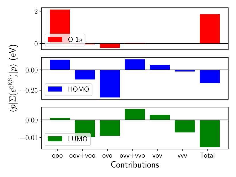
Figure 2: Decomposition of the $G3W2$ dynamical part into analytic terms for H₂O within pcSseg-3 basis based on PBEh(0.50). Expectation value for the O1$s$, the HOMO and the LUMO are given. Beware the change in y-axis scale.

Here we analyze the basic properties of the $G3W2$ self-energy for simple molecular systems. First, we concentrate on the analytic formula in Eqs. (13a-13f). While the computational scaling of all these terms is formally $N^{7}$, it is interesting to investigate the magnitude of each of these terms. In particular, in large basis sets, the number of virtual states $N_{v}$ is much larger than the number of occupied states $N_{o}$ and we expect that the term $\Sigma^{vvv}$ in Eq. (13b) will be the most expensive one to calculate.

In Fig. 2, we report the 6 terms in Eqs. (13a-13f) evaluated with PBEh(0.50) inputs for the water molecule (in the GW100 geometry ²⁰). We show the expectation value of the self-energies at the corresponding PBEh(0.50) eigenvalue, which is in general a very reasonable guess for valence states ⁵⁵ and core states ³⁵. While the total $G3W2$ self-energy is large for a core state ($\sim$ 2 eV), it is rather weak for the HOMO ($\sim$ 0.1 eV) and very weak for the LUMO ($\sim$ 0.01 eV).

For the core state, the term $\Sigma^{ooo}$ largely prevails. $\Sigma^{vov}$, $\Sigma^{ovv}+\Sigma^{vvo}$, and $\Sigma^{vvv}$ are hardly visible on the scale of our plot. They will be safely neglected in the core state evaluation in Section 3.5. Quite the opposite for valence electrons, the HOMO and LUMO states of H₂O have similar weights for all the contributions and then none of them can be neglected.

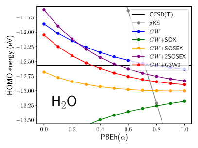
Figure 3: Starting point dependence of the HOMO quasiparticle energy for CO and H₂O with Def2-TZVPP basis set, for the different vertex approximation. The CCSD(T) reference ⁴⁷ is shown as an horizontal line.

The starting point dependence of one-shot $GW$ (i.e. $G_{0}W_{0}$) is well documented in the literature (see e.g. Ref. 16). The strong dependence of $GW$+SOSEX has also been studied by Ren and coworkers.⁷⁴. In Fig. 3 we analyze the starting point effect for all the vertex approximations mentioned in this work $GW$ (no vertex), $GW$+SOX, $GW$+SOSEX, $GW$+2SOSEX, $GW+G3W2$ for the HOMO energy of 2 molecules, CO and H₂O. To do so, we tune the content of exact-exchange $\alpha$ in PBEh functional from 0 to 1, with 0 giving the usual semi-local PBE functional and 0.25, PBE0. For all the studied approximations, the effect of the starting point is large. The PBE starting point, a terrible start for the quasiparticle energies of molecular systems, quite luckily induces a $GW$+SOSEX HOMO that compares well with CCSD(T). It is interesting to note that the $GW+G3W2$ curve is almost parallel to the $GW$ one: the $G3W2$ induces then a constant downward shift. However, for the starting points that yield good HOMO energies compared to $GW$ or to CCSD(T) ($\alpha\sim$ 0.50 – 0.75), the $G3W2$ correction brings the result away from the correct value. Only with a low value of $\alpha\sim 0.25$ can $GW+G3W2$ beat simple $GW$.

3.3 $GW$100 ionization potentials

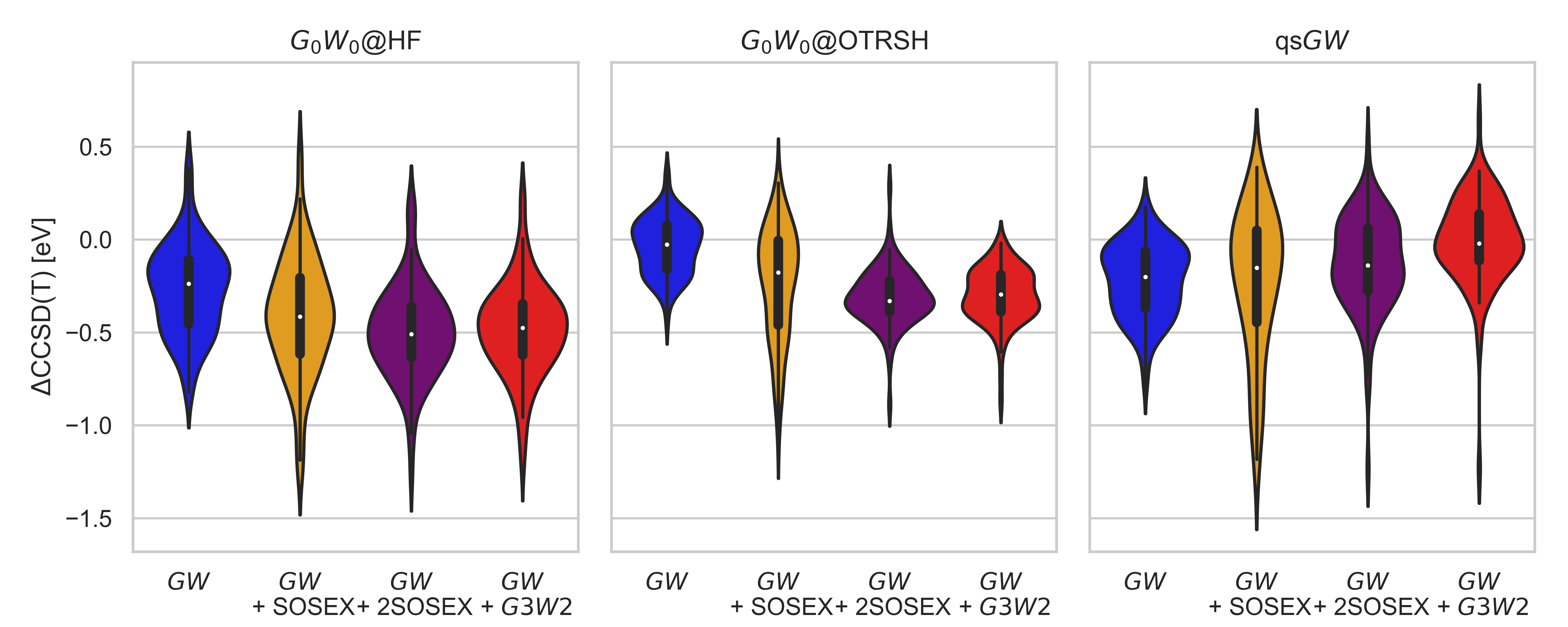
Figure 4: Errors of HOMO QP energies for $G_{0}W_{0}$ and different approximations of the $G3W2$ vertex correction with respect to CCSD(T) reference values ⁴⁷ for GW100 using HF and OTRSH starting points. All values are in eV.

	$GW$	$GW+$ SOSEX	$GW+$ 2SOSEX	$GW+G3W2$
HF	0.30	0.44	0.51	0.49
OTRSH	0.13	0.28	0.32	0.30
qs$GW$	0.23	0.32	0.21	0.17

Table 2: Mean absolute deviations of $G_{0}W_{0}$ and different approximations of the $G3W2$ vertex correction with respect to CCSD(T) reference values ⁴⁷ for GW100 using HF and OTRSH starting points. All values are in eV.

3.3.1 Generalized Kohn-Sham starting points

We focus first on the “one-shot” evaluation of the self-energy based on generalized Kohn-Sham. There are an infinite variations of Kohn-Sham starting points that could be used. Here we decide to concentrate on two remarkable ones: Hartree-Fock (HF) and optimally-tuned range-separated hybrid (OTRSH) ^{75, 76}. Firstly, HF is the most commonly used starting point for “post Hartree-Fock” methods in the quantum chemistry. Though not the most accurate choice, this approximation is useful for comparison and benchmarking. Secondly, OTRSH is less used in the literature however it has been shown recently to minimize the mean-error for $G_{0}W_{0}$ IPs for the GW100 set ⁷⁷. In the present work we use a PBE-based version of OTRSH ^{78, 79} where the short-range exchange is that of Henderson and coworkers ⁸⁰. The range-separation parameter $\gamma$ is determined so that the “$GW$ correction” vanishes as proposed in Ref. 77, while exact-exchange scaling parameters $\alpha=0.2$ and $\beta=0.8$ are kept constant.

Figure 4 shows the errors distributions of the $G_{0}W_{0}$, $G_{0}W_{0}$ + SOSEX, $G_{0}W_{0}$ + 2SOSEX and $G_{0}W_{0}+G3W2$ HOMO QP energies for HF and OTRSH starting points compared to the CCSD(T) reference values of Ref. 47 for the GW100 set. Mean absolute deviations (MAD) for all methods are shown in Table 2. With a MAD of 0.13 eV, $G_{0}W_{0}$@OTRSH is among the best performing $GW$ methods for the GW100 set⁷⁷ and any vertex corrections to the self-energy worsens the agreement with CCSD(T). The same observation can be made for $G_{0}W_{0}$@HF. For both starting points, the addition of SOSEX leads to higher IPs (more negative HOMOs) on average and also the spread of errors increases substantially, as can be seen from the distributions in Figure 4. Symmetric screening of the SOX term in the form of $G_{0}W_{0}$ + 2SOSEX slightly increases the average error compared to $G_{0}W_{0}$+SOSEX. However, it reduces the spread of the error again, indicating the 2SOSEX is a more consistent approximation to the full $G3W2$ term than SOSEX alone. Finally, the addition of the double frequency integral, leading to the full $G_{0}W_{0}+G3W2$ term, has only little effect on the MADs and the shape of the error distributions. This result has already been suggested by Figure 3 which shows that for large content of exchange $\alpha$, 2SOSEX and $G3W2$ give similar results. Also Table S2 ⁶⁷ shows that the contribution from the double frequency integral is typically of the order of only a few tens meV and only exceeds 100 meV in very few cases.

This observation suggests that 2SOSEX would be a consistent and suitable approximation to the complete $G3W2$ term. However, our data also clearly shows that it does not improve over $G_{0}W_{0}$.

3.3.2 Quasiparticle self-consistent $GW$ starting point

Turning to the qs$GW$ results shown in Fig. 4 we observe that the vertex correction shifts the qs$GW$ results in the opposite direction than for $G_{0}W_{0}$. qs$GW$ alone overestimates the CCSD(T) IPs, but qs$GW$ + $G3W2$ lowers them, bringing them in better agreement with the reference values. However, the vertex correction also produces clear outliers. One of them is Helium, one of the simplest systems in GW100, for which qs$GW$ + $G3W2$ deviates from CCSD(T) by more than 1.2 eV. This shows that $G3W2$ is also not a robust method to improve over qs$GW$. Our construction of the qs$GW$ Hamiltonian is based on ref. 70, even though alternative constructions have been shown to give slightly improved results for GW100.⁸¹

In Table S5⁶⁷ we also present results for qsGW₀ for a few selected systems, where $W$ is kept fixed after the first SCF cycle. These results show that the update of $W$, not the update of $G$ is responsible for the qualitatively different behavior of qs$GW$ compared to $G_{0}W_{0}$. As for $G_{0}W_{0}$, the $G3W2$ diagram increases the qsGW₀ IPs.

Finally, we notice that vertex corrections to qs$GW$ for periodic semi-conductors and insulators have so far only been investigated in the polarizability^{82, 83, 84, 85}. This is due to a well-known argument⁷⁰ that a non-interacting Green’s function behaves as an effective vertex correction to the self-energy. Therefore, the vertex should not be added to the self-energy to avoid that it is effectively double counted. Our results question the validity of this argument.

3.4 ACC24 ionization potentials and electron affinities

After having analyzed the $G3W2$ term for GW100, we turn to the ACC24 set⁵⁸ of 24 organic acceptor molecules with stable anions. This also allows for a meaningful comparison of LUMO QP energies and HOMO-LUMO gaps. We focus here on $G_{0}W_{0}$ based on the OTRSH starting point which has been shown to give very good results also for the ACC24 set.²¹

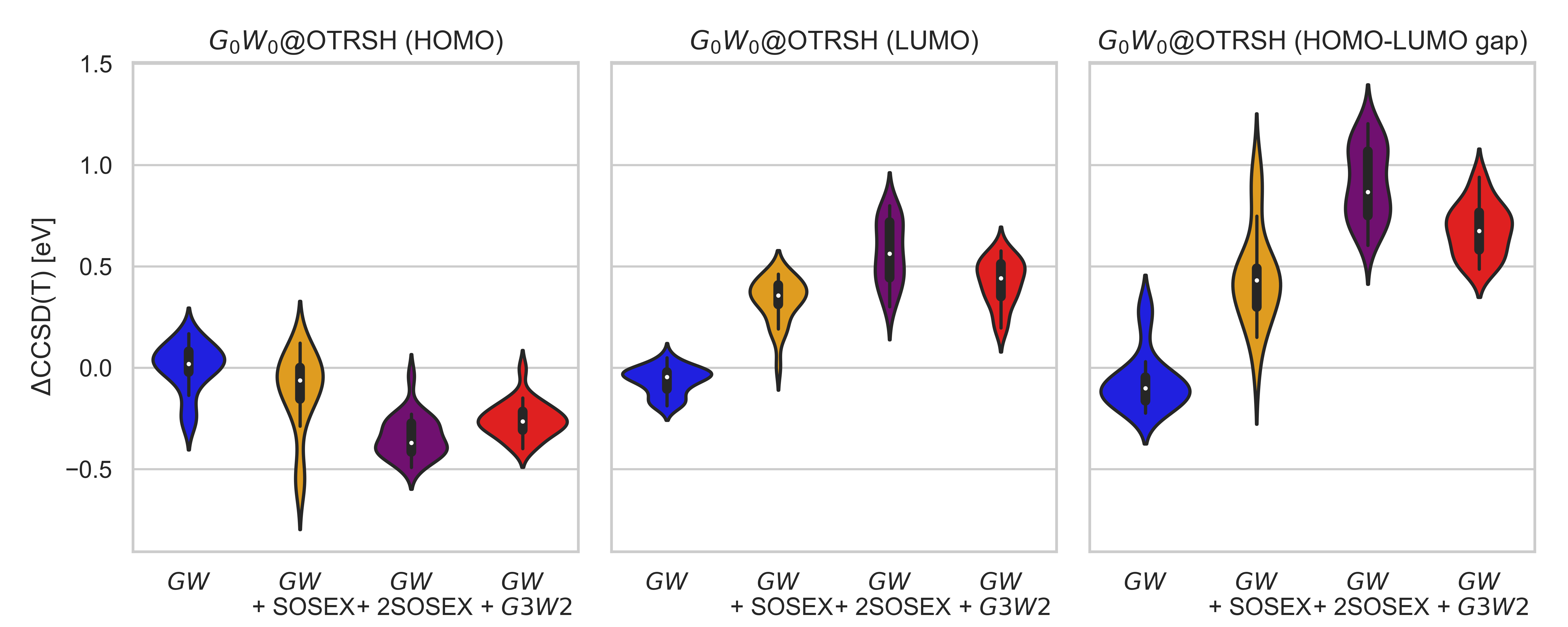
Figure 5: Errors of $G_{0}W_{0}$@OTRSH with different approximations of the $G3W2$ vertex correction with respect to CCSD(T) reference values for ACC24 for HOMO, LUMO and HOMO-LUMO gaps. All values are in eV. For some molecules, the $G3W2$ corrections have been performed using cc-pVTZ or aug-cc-pVDZ due to prohibitively high costs. See supporting information for details.

	$GW$	$GW+$ SOSEX	$GW+$ 2SOSEX	$GW+G3W2$
HOMO	0.09	0.15	0.34	0.26
LUMO	0.07	0.33	0.57	0.42
HOMO-LUMO gap	0.14	0.46	0.91	0.68

Table 3: Mean absolute deviations of $G_{0}W_{0}$@OTRSH and different approximations of the $G3W2$ vertex correction with respect to CCSD(T) reference values for ACC24 for HOMO, LUMO, and HOMO-LUMO gap. All values are in eV.

For the OTRSH starting point, Figure 4 shows the errors distributions of the $G_{0}W_{0}$, $G_{0}W_{0}$ + SOSEX, $G_{0}W_{0}$ + 2SOSEX and $G_{0}W_{0}+G3W2$ HOMO, LUMO and HOMO-LUMO gaps using against the CCSD(T) reference values of Ref. 58 for the ACC24 set. The corresponding MADs are shown in Table 3. We do not use the basis set limit extrapolated reference values from Ref. 58 but instead CCSD(T)/aug-cc-pVTZ results as reference. For the four molecules for which results with aug-cc-pVTZ are not available, we compare against CCSD(T)/aug-cc-pVDZ. We notice that also a comparison at the aug-cc-pVTZ does not eliminate basis set errors since the CCSD(T) converges faster to the complete basis set limit than $GW$ for individual QP energies.¹⁶ Only for HOMO-LUMO gaps, the rates of convergence are comparable.

Also, due to the high computational cost we calculate the vertex corrections at aug-cc-pVTZ for only about half of the 24 molecules while for the other we use either cc-pVTZ or aug-cc-pVDZ. For a discussion of the basis set limit convergence and details on the choice of basis for each system we refer to Tables S7 and S8. ⁶⁷ For the molecules for which we can afford aug-cc-pVTZ, we see that the results are almost identical to cc-pVTZ (MADs of 5-6 meV for HOMO and LUMO for the different vertex corrections). Also aug-cc-pVDZ is relatively close to TZ, with MADs of 60 meV for HOMO and 90 meV for LUMO for the full $G3W2$ correction. We therefore believe that this comparison reveals the qualitative behavior of the vertex corrections we test here.

For the HOMO energies we observe the same trend as for the GW100 set and notice that $G_{0}W_{0}$@OTRSH reproduces the CCSD(T) reference values with a MAD of 0.09 eV very well. The same can be observed for the LUMO energies. Here, the vertex corrections increase the LUMO energies considerably. In combination with the decreased HOMO energies, this leads to a major increase of the HOMO-LUMO gaps. The $G_{0}W_{0}$@OTRSH $+G3W2$ HOMO-LUMO gap has an average signed error of 0.68 eV, more than 0.5 eV worse than $G_{0}W_{0}$@OTRSH with 0.14 eV only.

3.5 Core levels

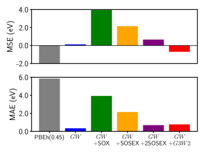
Figure 6: Mean signed deviation (upper panel) and mean absolute deviation (lower panel) in eV for 28 core state energies taken among the smallest molecules in CORE65 benchmark set ³⁵ evaluated within pc-Sseg-3 basis based on PBEh(0.45). This plot uses binding energies, which is the negative of the quasiparticle energies, as opposed to the rest of this study. Note that the PBEh(0.45) bars in gray are truncated for the sake of visualization.

Core level binding energies have been recently addressed in the framework of $GW$ ^{33, 34, 35}. We use the opportunity offered by the fully analytic expressions reported in Eqs. (13a)-(13f) to accurately evaluate $GW$ and $G3W2$ self-energies for core levels.

Building on the work of Meija-Rodriguez et. al. ⁸⁶, we employ an accurate basis set that was designed in particular to describe core electrons, namely pc-Sseg-3. Using Golze’s recommendation ³⁵, we evaluate the self-energy using a one-shot procedure based on PBEh(0.45). Relativistic corrections are added a posteriori with the values prescribed by Golze and coworkers ³⁵. In the CORE65 set ³, the reference binding energies are taken from various experiments.

The calculations based on the analytic approach to $G3W2$ are very demanding and hereafter we neglect the contributions to the self-energy that involve two or three virtual orbitals. We have seen in Sec. 3.2 that these terms are of the order of a few meV for core levels. Even with this approximation, the calculations remain challenging. Figure 6 reports the MSD and MAD for 28 core states out of the 65 energies gathered in the original CORE65 set. We have excluded the largest molecules because of computational burden and O₂ because of spin. The comprehensive results are given in Table S9 in the supplemental material⁶⁷.

From Figure 5, we see that $GW$ yields the best result and that $GW$+SOX deteriorates much. Gradually adding screening through SOSEX, 2SOSEX, and then full $G3W2$ goes in the correct direction. For core levels, the vertex corrections are indeed sizeable. It should be noted though, that the PBEh(0.45) starting point was specifically selected in Ref. 35 to minimize the $G_{0}W_{0}$ error. Tuning $\alpha$ in PBEh($\alpha$) could improve $GW+G3W2$. But such a study is beyond the scope of the present work.

4 Conclusion

In this work, we have derived and evaluated the formulas for the self-energy diagram drawn in Figure 1, which contains two dynamically screened Coulomb interactions $W(\omega)$ and three Green’s functions: this is the diagram named $G3W2$ by Kutepov ⁴⁵. We propose two formulas: a fully analytic one that is useful for analysis, reference and core levels and a numerical one that uses a double complex frequency quadrature that is more efficient for the HOMO-LUMO region.

Based on well-established molecular benchmarks for ionization potentials (GW100)²⁰, electron affinities (ACC24)²¹, and core levels (CORE65)³⁵, we conclude that in general the $GW+G3W2$ self-energy does not improve over the simpler $GW$ self-energy. When designing simpler semi-static approximations to $G3W2$, in the spirit of SOSEX ⁴⁸, we propose a new approximation that we name 2SOSEX that better approximates the complete $G3W2$ self-energy.

The strategy to keep the RPA screening and introduce vertex corrections only in the self-energy is certainly not sufficient. As already suggested long time ago by Del Sole and coworkers, vertex corrections in the self-energy should be combined with vertex corrections in $W$.⁴¹. This should be the subject of future investigation.

We acknowledge constructive discussions with Xinguo Ren and Patrick Rinke, aimed at clarifying that their equation (11) ⁴⁹ does not represent the exact expression corresponding to the complete second-order diagram. Part of this work was performed using HPC resources from GENCI–TGCC (Grant 2023-gen6018). AF acknowledges the use of supercomputer facilities at SURFsara sponsored by NWO Physical Sciences, with financial support from The Netherlands Organization for Scientific Research (NWO).

Individual results for each molecule in the GW100, ACC24, CORE65 benchmarks are made as Supporting information. Frequency grid convergence and comparison to FHI-AIMS results are also shown.

Appendix A Fourier-transforming $\Sigma^{G3W{{}_{p}}2}$ to real frequencies

This appendix shows all the steps to obtain the frequency-dependent expression of the dynamic part of the $G3W2$ self-energy, starting from the expression with times as obtained from Hedin’s equation.

Let us recall here Eq. (9):

$$\Sigma^{G3{W_{p}}2}(t_{1}-t_{2})=\mathrm{i}^{2}\int dt_{3}dt_{4}G(t_{1}-t_{4})W_{p}(t_{3}-t_{1})G(t_{4}-t_{3})W_{p}(t_{2}-t_{4})G(t_{3}-t_{2})$$ (19)

and let us introduce the difference time variables:

$$\tau = t_{1}-t_{2}$$ (20a)

$$\tau^{\prime} = t_{1}-t_{3}$$ (20b)

$$\tau^{\prime\prime} = t_{4}-t_{2}$$ (20c)

Combining these 3 variables, we obtain the other 3 needed time differences:

$$t_{1}-t_{4} = \tau-\tau^{\prime\prime}$$ (20d)

$$t_{4}-t_{3} = -\tau+\tau^{\prime}+\tau^{\prime\prime}$$ (20e)

$$t_{3}-t_{2} = \tau-\tau^{\prime}.$$ (20f)

Integration over $t_{3}$ and $t_{4}$ are then transformed to $\tau^{\prime}$ and $\tau^{\prime\prime}$ without other change:

$$\Sigma(\tau)=\mathrm{i}^{2}\int d\tau^{\prime}d\tau^{\prime\prime}G(\tau-\tau^{\prime\prime})W_{p}(-\tau^{\prime})G(-\tau+\tau^{\prime}+\tau^{\prime\prime})W_{p}(-\tau^{\prime\prime})G(\tau-\tau^{\prime}).$$ (21)

At the stage, we Fourier-transform all the times using the following definitions:

$$G(\omega)=\int d\tau e^{\mathrm{i}\omega\tau}G(\tau)$$ (22a)

and

$$G(\tau)=\frac{1}{2\pi}\int d\omega e^{-\mathrm{i}\omega\tau}G(\omega).$$ (22b)

$\Sigma$ is forward-transformed whereas the $G$ and the $W_{p}$ are backward-transformed:

$$\Sigma(\omega)=\frac{\mathrm{i}^{2}}{(2\pi)^{5}}\int d\tau d\tau^{\prime}d\tau^{\prime\prime}e^{\mathrm{i}\omega\tau}\int d\omega_{1}d\omega^{\prime}d\omega_{2}d\omega^{\prime\prime}d\omega_{3}\\ \times e^{-\mathrm{i}\omega_{1}(\tau-\tau^{\prime\prime})}e^{+\mathrm{i}\omega^{\prime}\tau^{\prime}}e^{-\mathrm{i}\omega_{2}(-\tau+\tau^{\prime}+\tau^{\prime\prime})}e^{+\mathrm{i}\omega^{\prime\prime}\tau^{\prime\prime}}e^{-\mathrm{i}\omega_{3}(\tau-\tau^{\prime})}\\ \times G(\omega_{1})W_{p}(\omega^{\prime})G(\omega_{2})W_{p}(\omega^{\prime\prime})G(\omega_{3})$$ (23)

Performing the integrals over $\tau,\tau^{\prime},\tau^{\prime\prime}$ variables yields 3 $\delta$ functions:

$$\int d\tau e^{\mathrm{i}\tau(\omega-\omega_{1}+\omega_{2}-\omega_{3})} = 2\pi\delta(\omega-\omega_{1}+\omega_{2}-\omega_{3})$$ (24a)

$$\int d\tau^{\prime}e^{\mathrm{i}\tau^{\prime}(\omega^{\prime}-\omega_{2}+\omega_{3})} = 2\pi\delta(\omega^{\prime}-\omega_{2}+\omega_{3})$$ (24b)

$$\int d\tau^{\prime\prime}e^{\mathrm{i}\tau^{\prime\prime}(\omega^{\prime\prime}+\omega_{1}-\omega_{2})} = 2\pi\delta(\omega^{\prime\prime}+\omega_{1}-\omega_{2}).$$ (24c)

This allows one to eliminate $\omega_{1}$, $\omega_{2}$, and $\omega_{3}$:

$$\omega_{1} = \omega+\omega^{\prime}$$ (25a)

$$\omega_{2} = \omega+\omega^{\prime}+\omega^{\prime\prime}$$ (25b)

$$\omega_{3} = \omega\phantom{+\omega^{\prime}}~{}\,+\omega^{\prime\prime}.$$ (25c)

Finally, this yield the result announced in the main text in Eq. (10):

$$\Sigma^{G3W{{}_{p}}2}(\omega)=\left(\frac{\mathrm{i}}{2\pi}\right)^{2}\int d\omega^{\prime}\int d\omega^{\prime\prime}G(\omega+\omega^{\prime})W_{p}(\omega^{\prime})G(\omega+\omega^{\prime}+\omega^{\prime\prime})W_{p}(\omega^{\prime\prime})G(\omega+\omega^{\prime\prime}).$$ (26)

Appendix B Analytic calculation of $\Sigma^{ooo}$

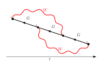
Figure 7: Goldstone-Feynman diagram for $\Sigma^{ooo}$.

In this appendix, we write the step-by-step derivation of the part of the self-energy that involves 3 occupied MO in $G$, labeled $i$, $j$, $k$ and 2 resonant poles in $W_{p}$, labeled $t$ and $s$. The corresponding Feynman-Goldstone diagram is drawn in Figure 7, where the time arrow is shown. The analytic expression of this diagram involve the following frequency parts:

$$\frac{\mathrm{i}}{2\pi}\int d\omega^{\prime}\frac{\mathrm{i}}{2\pi}\int d\omega^{\prime\prime}\frac{1}{\omega+\omega^{\prime}-\epsilon_{i}-\mathrm{i}\eta}\times\frac{1}{\omega^{\prime}-\Omega_{t}+\mathrm{i}\eta}\\ \times\frac{1}{\omega+\omega^{\prime}+\omega^{\prime\prime}-\epsilon_{j}-\mathrm{i}\eta}\times\frac{1}{\omega^{\prime\prime}-\Omega_{s}+\mathrm{i}\eta}\times\frac{1}{\omega+\omega^{\prime\prime}-\epsilon_{k}-\mathrm{i}\eta}$$ (27)

First we perform the integral $\frac{\mathrm{i}}{2\pi}\int d\omega^{\prime\prime}$ using the residue theorem. We draw a contour consisting the real axis and an arc below the real axis. This contour encloses the poles with negative imaginary part and there is only one: $\omega^{\prime\prime}=\Omega_{s}-\mathrm{i}\eta$. The residue theorem then gives

$$-2\pi\mathrm{i}\frac{1}{\omega+\omega^{\prime}+\Omega_{s}-\epsilon_{j}-2\mathrm{i}\eta}\times\frac{1}{\omega+\Omega_{s}-\epsilon_{k}-2\mathrm{i}\eta}.$$ (28)

The leading negative sign comes from the anticlockwise closing of the contour. The second term in Eq. (28) has no $\omega^{\prime}$ dependence and is a simple prefactor.

Second we have to perform the integral over $\omega^{\prime}$:

$$\frac{\mathrm{i}}{2\pi}\int d\omega^{\prime}\frac{1}{\omega+\omega^{\prime}-\epsilon_{i}-\mathrm{i}\eta}\times\frac{1}{\omega^{\prime}-\Omega_{t}+\mathrm{i}\eta}\times\frac{1}{\omega+\omega^{\prime}+\Omega_{s}-\epsilon_{j}-2\mathrm{i}\eta}.$$ (29)

The first two factors come from Eq. (27) and the last one from Eq. (28).

We use the residue theorem again with a contour consisting of the real axis and an arc in the lower part of the complex plane. The contour is oriented anticlockwise. There is only one pole with a negative imaginary part: $\omega^{\prime}=\Omega_{t}-\mathrm{i}\eta$. The application of the residue theorem reads

$$-2\pi\mathrm{i}\frac{1}{\omega+\Omega_{t}-\epsilon_{i}-2\mathrm{i}\eta}\times\frac{1}{\omega+\Omega_{t}+\Omega_{s}-\epsilon_{j}-3\mathrm{i}\eta}.$$ (30)

Gathering the two factors in Eq. (30) and the last factor in Eq. (28), we obtain the complete frequency dependence:

$$\frac{1}{\omega-\epsilon_{i}+\Omega_{t}-2\mathrm{i}\eta}\times\frac{1}{\omega-\epsilon_{j}+\Omega_{t}+\Omega_{s}-3\mathrm{i}\eta}\times\frac{1}{\omega-\epsilon_{k}+\Omega_{s}-2\mathrm{i}\eta}.$$ (31)

Now inserting the correct spatial numerators, we get the final expression for $\Sigma_{pq}^{ooo}(\omega)$:

$$\Sigma_{pq}^{ooo}(\omega)=\sum_{ts}\sum_{ijk}\frac{w_{t}^{pi}\cdot w_{t}^{jk}\cdot w_{s}^{qk}\cdot w_{s}^{ij}}{(\omega-\epsilon_{i}+\Omega_{t}-2\mathrm{i}\eta)\cdot(\omega-\epsilon_{j}+\Omega_{t}+\Omega_{s}-3\mathrm{i}\eta)\cdot(\omega-\epsilon_{k}+\Omega_{s}-2\mathrm{i}\eta)}.$$ (32)

This is the complete occupied-occupied-occupied self-energy. Indeed, the other terms that involve anti-resonant excitations in $W_{p}$ have all the poles located in the same upper-half of the complex plan and therefore vanish.

Appendix C Fourier-transforming $\Sigma^{G3W{{}_{p}}2}$ to imaginary frequencies

The derivation of (14) is very similar to the derivation of (10) described in detail in appendix A. The only difference is than one needs to work with Laplace transforms which connect the real time axis to the complex plane. While these expressions are generally not unique, we choose a definition which matches the expression often used in space-time formulations of $GW$⁶¹

$$G(\mu+\mathrm{i}\omega)=\mathrm{i}\int^{\infty}_{-\infty}e^{-(\mu+\mathrm{i}\omega)\tau}G(\tau)d\tau$$ (33a)

$$G(\tau)=-\frac{\mathrm{i}}{2\pi}\int^{\infty}_{-\infty}e^{(\mu+\mathrm{i}\omega)\tau}G(\mu+\mathrm{i}\omega)d\omega\;.$$ (33b)

$\tau$ is a real time argument. Both transformations are well-defined as long as $\mu$ separates the HOMO and LUMO energies. Consistent with these definitions, the imaginary-frequency single-particle Green’s function can be defined by

$$G(\mathbf{r},\mathbf{r}^{\prime},\mu+\mathrm{i}\omega)=\sum_{p}\frac{\phi_{p}(\mathbf{r})\phi^{*}_{p}(\mathbf{r}^{\prime})}{\mu+\mathrm{i}\omega-\epsilon_{p}}\;.$$ (34)

To arrive at (14), one starts from (21) and forward transforms $\Sigma$ using (33), while all $G$ and $W_{p}$ are backward-transformed. One then arrives at (omitting spatial indices for brevity)

$$\Sigma^{G3W2}(\mu+\mathrm{i}\omega)=\left(\frac{-1}{2\pi}\right)^{2}\int d\omega^{\prime}d\omega^{\prime\prime} G(\mu+\mathrm{i}\omega+\mathrm{i}\omega^{\prime})G(\mu+\mathrm{i}\omega+\mathrm{i}\omega^{\prime}+\mathrm{i}\omega^{\prime\prime})$$ (35)

$$\times G(\mu+\mathrm{i}\omega+\mathrm{i}\omega^{\prime\prime})W(\mathrm{i}\omega^{\prime})W(\mathrm{i}\omega^{\prime\prime})\;,$$

and using (34) for all $G$ one arrives at (14).

References

- Hedin 1965 Hedin, L. New Method for Calculating the One-Particle Green’s Function with Application to the Electron-Gas Problem. Phys. Rev. 1965, 139, A796–A823
- Reining 2018 Reining, L. The GW approximation: content, successes and limitations. Wiley Interdisciplinary Reviews: Computational Molecular Science 2018, 8, e1344
- Golze et al. 2019 Golze, D.; Dvorak, M.; Rinke, P. The GW Compendium: A Practical Guide to Theoretical Photoemission Spectroscopy. Frontiers in Chemistry 2019, 7, 377
- Lundqvist 1967 Lundqvist, B. Single-particle spectrum of the degenerate electron gas. Physik der Kondensierten Materie 1967, 6, 193–205
- Strinati et al. 1980 Strinati, G.; Mattausch, H. J.; Hanke, W. Dynamical Correlation Effects on the Quasiparticle Bloch States of a Covalent Crystal. Phys. Rev. Lett. 1980, 45, 290–294
- Hybertsen and Louie 1985 Hybertsen, M. S.; Louie, S. G. First-Principles Theory of Quasiparticles: Calculation of Band Gaps in Semiconductors and Insulators. Phys. Rev. Lett. 1985, 55, 1418–1421
- Godby et al. 1986 Godby, R. W.; Schlüter, M.; Sham, L. J. Accurate Exchange-Correlation Potential for Silicon and Its Discontinuity on Addition of an Electron. Phys. Rev. Lett. 1986, 56, 2415–2418
- Shirley and Martin 1993 Shirley, E. L.; Martin, R. M. quasiparticle calculations in atoms. Phys. Rev. B 1993, 47, 15404–15412
- Grossman et al. 2001 Grossman, J. C.; Rohlfing, M.; Mitas, L.; Louie, S. G.; Cohen, M. L. High Accuracy Many-Body Calculational Approaches for Excitations in Molecules. Phys. Rev. Lett. 2001, 86, 472–475
- Rostgaard et al. 2010 Rostgaard, C.; Jacobsen, K. W.; Thygesen, K. S. Fully self-consistent GW calculations for molecules. Phys. Rev. B 2010, 81, 085103
- Blase et al. 2011 Blase, X.; Attaccalite, C.; Olevano, V. First-principles calculations for fullerenes, porphyrins, phtalocyanine, and other molecules of interest for organic photovoltaic applications. Phys. Rev. B 2011, 83, 115103
- Bruneval 2012 Bruneval, F. Ionization energy of atoms obtained from self-energy or from random phase approximation total energies. J. Chem. Phys. 2012, 136, 194107
- Ren et al. 2012 Ren, X.; Rinke, P.; Blum, V.; Wieferink, J.; Tkatchenko, A.; Sanfilippo, A.; Reuter, K.; Scheffler, M. Resolution-of-identity approach to Hartree–Fock, hybrid density functionals, RPA, MP2 and GW with numeric atom-centered orbital basis functions. New Journal of Physics 2012, 14, 053020
- Sharifzadeh et al. 2012 Sharifzadeh, S.; Tamblyn, I.; Doak, P.; Darancet, P.; Neaton, J. Quantitative molecular orbital energies within a G0W0 approximation. Europ. Phys. J. B 2012, 85, 323
- Körzdörfer and Marom 2012 Körzdörfer, T.; Marom, N. Strategy for finding a reliable starting point for demonstrated for molecules. Phys. Rev. B 2012, 86, 041110
- Bruneval and Marques 2013 Bruneval, F.; Marques, M. A. L. Benchmarking the Starting Points of the GW Approximation for Molecules. J. Chem. Theory Comput. 2013, 9, 324–329
- van Setten et al. 2013 van Setten, M. J.; Weigend, F.; Evers, F. The GW-Method for Quantum Chemistry Applications: Theory and Implementation. J. Chem. Theory Comput. 2013, 9, 232–246, PMID: 26589026
- Koval et al. 2014 Koval, P.; Foerster, D.; Sánchez-Portal, D. Fully self-consistent and quasiparticle self-consistent for molecules. Phys. Rev. B 2014, 89, 155417
- Govoni and Galli 2015 Govoni, M.; Galli, G. Large Scale GW Calculations. J. Chem. Theory Comput. 2015, 11, 2680–2696, PMID: 26575564
- van Setten et al. 2015 van Setten, M. J.; Caruso, F.; Sharifzadeh, S.; Ren, X.; Scheffler, M.; Liu, F.; Lischner, J.; Lin, L.; Deslippe, J. R.; Louie, S. G.; Yang, C.; Weigend, F.; Neaton, J. B.; Evers, F.; Rinke, P. GW100: Benchmarking G0W0 for Molecular Systems. J. Chem. Theory Comput. 2015, 11, 5665–5687, PMID: 26642984
- Knight et al. 2016 Knight, J. W.; Wang, X.; Gallandi, L.; Dolgounitcheva, O.; Ren, X.; Ortiz, J. V.; Rinke, P.; Körzdörfer, T.; Marom, N. Accurate Ionization Potentials and Electron Affinities of Acceptor Molecules III: A Benchmark of GW Methods. Journal of Chemical Theory and Computation 2016, 12, 615–626
- Kuwahara et al. 2016 Kuwahara, R.; Noguchi, Y.; Ohno, K. Bethe-Salpeter equation approach for photoabsorption spectra: Importance of self-consistent calculations in small atomic systems. Phys. Rev. B 2016, 94, 121116
- Blase et al. 2016 Blase, X.; Boulanger, P.; Bruneval, F.; Fernandez-Serra, M.; Duchemin, I. and Bethe-Salpeter study of small water clusters. J. Chem. Phys. 2016, 144, 034109
- Heßelmann 2017 Heßelmann, A. Ionization energies and electron affinities from a random-phase-approximation many-body Green’s-function method including exchange interactions. Phys. Rev. A 2017, 95, 062513
- Maggio et al. 2017 Maggio, E.; Liu, P.; van Setten, M. J.; Kresse, G. GW100: A Plane Wave Perspective for Small Molecules. Journal of Chemical Theory and Computation 2017, 13, 635–648
- Vlček et al. 2017 Vlček, V.; Rabani, E.; Neuhauser, D.; Baer, R. Stochastic GW Calculations for Molecules. J. Chem. Theory Comput. 2017, 13, 4997–5003
- Vlček et al. 2018 Vlček, V.; Li, W.; Baer, R.; Rabani, E.; Neuhauser, D. Swift GW beyond 10,000 electrons using sparse stochastic compression. Phys. Rev. B 2018, 98, 075107
- Lange and Berkelbach 2018 Lange, M. F.; Berkelbach, T. C. On the Relation between Equation-of-Motion Coupled-Cluster Theory and the GW Approximation. J. Chem. Theory Comput. 2018, 14, 4224–4236
- Wilhelm et al. 2018 Wilhelm, J.; Golze, D.; Talirz, L.; Hutter, J.; Pignedoli, C. A. Toward GW Calculations on Thousands of Atoms. JPCL 2018, 9, 306–312
- Véril et al. 2018 Véril, M.; Romaniello, P.; Berger, J. A.; Loos, P.-F. Unphysical Discontinuities in GW Methods. J. Chem. Theory Comput. 2018, 14, 5220–5228, PMID: 30212627
- Förster and Visscher 2020 Förster, A.; Visscher, L. Low-Order Scaling G0W0 by Pair Atomic Density Fitting. J. Chem. Theory Comput. 2020, 16, 7381–7399, PMID: 33174743
- Bintrim and Berkelbach 2021 Bintrim, S. J.; Berkelbach, T. C. Full-frequency GW without frequency. J. Chem. Phys. 2021, 154, 041101
- Golze et al. 2018 Golze, D.; Wilhelm, J.; van Setten, M. J.; Rinke, P. Core-Level Binding Energies from GW: An Efficient Full-Frequency Approach within a Localized Basis. Journal of Chemical Theory and Computation 2018, 14, 4856–4869, PMID: 30092140
- van Setten et al. 2018 van Setten, M. J.; Costa, R.; Viñes, F.; Illas, F. Assessing GW Approaches for Predicting Core Level Binding Energies. J. Chem. Theory Comput. 2018, 14, 877–883
- Golze et al. 2020 Golze, D.; Keller, L.; Rinke, P. Accurate Absolute and Relative Core-Level Binding Energies from GW. J. Phys. Chem. Lett. 2020, 11, 1840–1847, PMID: 32043890
- Hedin and Lundqvist 1970 Hedin, L.; Lundqvist, S. In ; Frederick Seitz, D. T., Ehrenreich, H., Eds.; Solid State Physics; Academic Press, 1970; Vol. 23; pp 1 – 181
- Northrup et al. 1987 Northrup, J. E.; Hybertsen, M. S.; Louie, S. G. Theory of quasiparticle energies in alkali metals. Phys. Rev. Lett. 1987, 59, 819–822
- Bruneval et al. 2005 Bruneval, F.; Sottile, F.; Olevano, V.; Del Sole, R.; Reining, L. Many-Body Perturbation Theory Using the Density-Functional Concept: Beyond the Approximation. Phys. Rev. Lett. 2005, 94, 186402
- Shishkin et al. 2007 Shishkin, M.; Marsman, M.; Kresse, G. Accurate Quasiparticle Spectra from Self-Consistent GW Calculations with Vertex Corrections. Phys. Rev. Lett. 2007, 99, 246403
- Lewis and Berkelbach 2019 Lewis, A. M.; Berkelbach, T. C. Vertex Corrections to the Polarizability Do Not Improve the GW Approximation for the Ionization Potential of Molecules. J. Chem. Theory Comput. 2019, 15, 2925–2932, PMID: 30933508
- Del Sole et al. 1994 Del Sole, R.; Reining, L.; Godby, R. W. GW approximation for electron self-energies in semiconductors and insulators. Phys. Rev. B 1994, 49, 8024–8028
- Maggio and Kresse 2017 Maggio, E.; Kresse, G. GW Vertex Corrected Calculations for Molecular Systems. J. Chem. Theory Comput. 2017, 13, 4765–4778
- Vlček 2019 Vlček, V. Stochastic Vertex Corrections: Linear Scaling Methods for Accurate Quasiparticle Energies. J. Chem. Theory Comput. 2019, 15, 6254–6266
- Mejuto-Zaera et al. 2021 Mejuto-Zaera, C.; Weng, G.; Romanova, M.; Cotton, S. J.; Whaley, K. B.; Tubman, N. M.; Vlček, V. Are multi-quasiparticle interactions important in molecular ionization? J. Chem. Phys. 2021, 154, 121101
- Kutepov 2021 Kutepov, A. L. Spatial non-locality of electronic correlations beyond GW approximation. J. Phys. Condens. Matter 2021, 33, 485601
- Szabó and Ostlund 1996 Szabó, A.; Ostlund, N. S. Modern quantum chemistry : introduction to advanced electronic structure theory; Dover Publications: Mineola (N.Y.), 1996
- Bruneval et al. 2021 Bruneval, F.; Dattani, N.; van Setten, M. J. The GW Miracle in Many-Body Perturbation Theory for the Ionization Potential of Molecules. Frontiers in Chemistry 2021, 9
- Ren et al. 2015 Ren, X.; Marom, N.; Caruso, F.; Scheffler, M.; Rinke, P. Beyond the approximation: A second-order screened exchange correction. Phys. Rev. B 2015, 92, 081104
- Wang et al. 2021 Wang, Y.; Rinke, P.; Ren, X. Assessing the G0W0Gamma0(1) Approach: Beyond G0W0 with Hedin’s Full Second-Order Self-Energy Contribution. J. Chem. Theory Comput. 2021, 17, 5140–5154, PMID: 34319724
- Grüneis et al. 2014 Grüneis, A.; Kresse, G.; Hinuma, Y.; Oba, F. Ionization Potentials of Solids: The Importance of Vertex Corrections. Phys. Rev. Lett. 2014, 112, 096401
- Förster and Visscher 2022 Förster, A.; Visscher, L. Exploring the statically screened correction to the self-energy: Charged excitations and total energies of finite systems. Phys. Rev. B 2022, 105, 125121
- Förster et al. 2023 Förster, A.; van Lenthe, E.; Spadetto, E.; Visscher, L. Two-component $GW$ calculations: Cubic scaling implementation and comparison of partially self-consistent variants. J. Chem. Theory Comput. 2023, 19, 5958–5976
- Stefanucci et al. 2014 Stefanucci, G.; Pavlyukh, Y.; Uimonen, A.-M.; van Leeuwen, R. Diagrammatic expansion for positive spectral functions beyond : Application to vertex corrections in the electron gas. Phys. Rev. B 2014, 90, 115134
- Pavlyukh et al. 2016 Pavlyukh, Y.; Uimonen, A.-M.; Stefanucci, G.; van Leeuwen, R. Vertex Corrections for Positive-Definite Spectral Functions of Simple Metals. Phys. Rev. Lett. 2016, 117, 206402
- Bruneval et al. 2016 Bruneval, F.; Rangel, T.; Hamed, S. M.; Shao, M.; Yang, C.; Neaton, J. B. Molgw 1: Many-body perturbation theory software for atoms, molecules, and clusters. Comput. Phys. Commun. 2016, 208, 149 – 161
- Te Velde and Baerends 1991 Te Velde, G.; Baerends, E. J. Precise density-functional method for periodic structures. Phys. Rev. B 1991, 44, 7888–7903
- Philipsen et al. 2022 Philipsen, P.; te Velde, G.; Baerends, E.; Berger, J.; de Boeij, P.; Franchini, M.; Groeneveld, J.; Kadantsev, E.; Klooster, R.; Kootstra, F.; Pols, M.; Romaniello, P.; Raupach, M.; Skachkov, D.; Snijders, J.; Verzijl, C.; Gil, J. C.; Thijssen, J. M.; Wiesenekker, G.; Peeples, C. A.; Schreckenbach, G.; Ziegler., T. BAND 2022.1 (modified development version), SCM, Theoretical Chemistry, Vrije Universiteit, Amsterdam, The Netherlands, http://www.scm.com. 2022
- Richard et al. 2016 Richard, R. M.; Marshall, M. S.; Dolgounitcheva, O.; Ortiz, J. V.; Brédas, J.-L.; Marom, N.; Sherrill, C. D. Accurate Ionization Potentials and Electron Affinities of Acceptor Molecules I. Reference Data at the CCSD(T) Complete Basis Set Limit. J. Chem. Theory Comput. 2016, 12, 595–604
- Strinati 1988 Strinati, G. Application of the greens-functions method to the study of the optical-properties of semiconductors. Riv. Nuovo Cimento 1988, 11, 1
- Tiago and Chelikowsky 2006 Tiago, M. L.; Chelikowsky, J. R. Optical excitations in organic molecules, clusters, and defects studied by first-principles Green’s function methods. Phys. Rev. B 2006, 73, 205334
- Rieger et al. 1999 Rieger, M. M.; Steinbeck, L.; White, I.; Rojas, H.; Godby, R. The GW space-time method for the self-energy of large systems. Comput. Phys. Commun. 1999, 117, 211–228
- Liu et al. 2016 Liu, P.; Kaltak, M.; Klimeš, J. c. v.; Kresse, G. Cubic scaling : Towards fast quasiparticle calculations. Phys. Rev. B 2016, 94, 165109
- Rojas et al. 1995 Rojas, H. N.; Godby, R. W.; Needs, R. J. Space-Time Method for Ab Initio Calculations of Self-Energies and Dielectric Response Functions of Solids. Phys. Rev. Lett. 1995, 74, 1827–1830
- Lebègue et al. 2003 Lebègue, S.; Arnaud, B.; Alouani, M.; Bloechl, P. E. Implementation of an all-electron approximation based on the projector augmented wave method without plasmon pole approximation: Application to Si, SiC, AlAs, InAs, NaH, and KH. Phys. Rev. B 2003, 67, 155208
- Yang et al. 2007 Yang, R.; Rendell, A. P.; Frisch, M. J. Automatically generated Coulomb fitting basis sets: Design and accuracy for systems containing H to Kr. J. Chem. Phys. 2007, 127, 074102
- Frisch et al. 2016 Frisch, M. J.; Trucks, G. W.; Schlegel, H. B.; Scuseria, G. E.; Robb, M. A.; Cheeseman, J. R.; Scalmani, G.; Barone, V.; Petersson, G. A.; Nakatsuji, H.; Li, X.; Caricato, M.; Marenich, A. V.; Bloino, J.; Janesko, B. G.; Gomperts, R.; Mennucci, B.; Hratchian, H. P.; Ortiz, J. V.; Izmaylov, A. F.; Sonnenberg, J. L.; Williams-Young, D.; Ding, F.; Lipparini, F.; Egidi, F.; Goings, J.; Peng, B.; Petrone, A.; Henderson, T.; Ranasinghe, D.; Zakrzewski, V. G.; Gao, J.; Rega, N.; Zheng, G.; Liang, W.; Hada, M.; Ehara, M.; Toyota, K.; Fukuda, R.; Hasegawa, J.; Ishida, M.; Nakajima, T.; Honda, Y.; Kitao, O.; Nakai, H.; Vreven, T.; Throssell, K.; Montgomery, J. A., Jr.; Peralta, J. E.; Ogliaro, F.; Bearpark, M. J.; Heyd, J. J.; Brothers, E. N.; Kudin, K. N.; Staroverov, V. N.; Keith, T. A.; Kobayashi, R.; Normand, J.; Raghavachari, K.; Rendell, A. P.; Burant, J. C.; Iyengar, S. S.; Tomasi, J.; Cossi, M.; Millam, J. M.; Klene, M.; Adamo, C.; Cammi, R.; Ochterski, J. W.; Martin, R. L.; Morokuma, K.; Farkas, O.; Foresman, J. B.; Fox, D. J. Gaussian˜16 Revision B.01. 2016; Gaussian Inc. Wallingford CT
- 67 See supporting information at [URL will be inserted by publisher] for the grid convergence, for comparison with FHI-AIMS results, and for the list of individual molecule results in the GW100, ACC24, and CORE65 benchmarks
- Faleev et al. 2004 Faleev, S. V.; van Schilfgaarde, M.; Kotani, T. All-electron self-consistent GW approximation: Application to Si, MnO, and NiO. Phys. Rev. Lett. 2004, 93, 126406
- van Schilfgaarde et al. 2006 van Schilfgaarde, M.; Kotani, T.; Faleev, S. Quasiparticle self-consistent GW theory. Phys. Rev. Lett. 2006, 96, 226402
- Kotani et al. 2007 Kotani, T.; van Schilfgaarde, M.; Faleev, S. V. Quasiparticle self-consistent GW method: A basis for the independent-particle approximation. Phys. Rev. B 2007, 76, 165106
- Förster and Visscher 2021 Förster, A.; Visscher, L. Low-Order Scaling Quasiparticle Self-Consistent GW for Molecules. Front. Chem. 2021, 9, 736591
- Spadetto et al. 2023 Spadetto, E.; Philipsen, P. H. T.; Förster, A.; Visscher, L. Toward Pair Atomic Density Fitting for Correlation Energies with Benchmark Accuracy. J. Chem. Theory Comput. 2023, 19, 1499–1516
- Erhard et al. 2022 Erhard, J.; Fauser, S.; Trushin, E.; Görling, A. Scaled -functionals for the Kohn–Sham correlation energy with scaling functions from the homogeneous electron gas. J. Chem. Phys. 2022, 157, 114105
- Ren et al. 2013 Ren, X.; Rinke, P.; Scuseria, G. E.; Scheffler, M. Renormalized second-order perturbation theory for the electron correlation energy: Concept, implementation, and benchmarks. Phys. Rev. B 2013, 88, 035120
- Baer and Neuhauser 2005 Baer, R.; Neuhauser, D. Density Functional Theory with Correct Long-Range Asymptotic Behavior. Phys. Rev. Lett. 2005, 94, 043002
- Livshits and Baer 2007 Livshits, E.; Baer, R. A well-tempered density functional theory of electrons in molecules. Phys. Chem. Chem. Phys. 2007, 9, 2932–2941
- McKeon et al. 2022 McKeon, C. A.; Hamed, S. M.; Bruneval, F.; Neaton, J. B. An optimally tuned range-separated hybrid starting point for ab initio GW plus Bethe-Salpeter equation calculations of molecules. J. Chem. Phys. 2022, 157, 074103
- Refaely-Abramson et al. 2012 Refaely-Abramson, S.; Sharifzadeh, S.; Govind, N.; Autschbach, J.; Neaton, J. B.; Baer, R.; Kronik, L. Quasiparticle Spectra from a Nonempirical Optimally Tuned Range-Separated Hybrid Density Functional. Phys. Rev. Lett. 2012, 109, 226405
- Kronik et al. 2012 Kronik, L.; Stein, T.; Refaely-Abramson, S.; Baer, R. Excitation Gaps of Finite-Sized Systems from Optimally Tuned Range-Separated Hybrid Functionals. J. Chem. Theory Comput. 2012, 8, 1515–1531
- Henderson et al. 2008 Henderson, T. M.; Janesko, B. G.; Scuseria, G. E. Generalized gradient approximation model exchange holes for range-separated hybrids. J. Chem. Phys. 2008, 128, 194105
- Marie and Loos 2023 Marie, A.; Loos, P.-F. A Similarity Renormalization Group Approach to Green’s Function Methods. J. Chem. Theory Comput. 2023, 19, 3943
- Cunningham et al. 2018 Cunningham, B.; Grüning, M.; Azarhoosh, P.; Pashov, D.; van Schilfgaarde, M. Effect of ladder diagrams on optical absorption spectra in a quasiparticle self-consistent GW framework. Phys. Rev. Mater. 2018, 2, 034603
- Cunningham et al. 2021 Cunningham, B.; Gruening, M.; Pashov, D.; van Schilfgaarde, M. QSGW: Quasiparticle Self consistent GW with ladder diagrams in W. arXiv:2106.05759v1 2021,
- Tal et al. 2021 Tal, A.; Chen, W.; Pasquarello, A. Vertex function compliant with the Ward identity for quasiparticle self-consistent calculations beyond GW. Phys. Rev. B 2021, 103, 161104
- Lorin et al. 2023 Lorin, A.; Bischoff, T.; Tal, A.; Pasquarello, A. Band alignments through quasiparticle self-consistent GW with efficient vertex corrections. Phys. Rev. B 2023, 108, 245303
- Mejia-Rodriguez et al. 2022 Mejia-Rodriguez, D.; Kunitsa, A.; Aprà, E.; Govind, N. Basis Set Selection for Molecular Core-Level GW Calculations. J. Chem. Theory Comput. 2022, 18, 4919–4926, PMID: 35816679