An Efficient Algorithm for Spatial-Spectral Partial Volume Compartment Mapping with Applications to Multicomponent Diffusion and Relaxation MRI

Abstract

It has been previously shown that high-quality partial volume tissue compartment maps can be obtained by combining multiparametric contrast-encoded MRI data acquisition methods with spatially-regularized spectroscopic image estimation techniques. However, the advantages of this combined approach generally come at the expense of substantial computational complexity. In this work, we propose a new algorithm to solve this kind of estimation problem more efficiently. Our algorithm is based on the linearized alternating directions method of multipliers (LADMM), and relies on the introduction of novel quadratic penalty terms to substantially simplify the subproblems that must be solved at each iteration. We evaluate this algorithm on a variety of different estimation problems (diffusion-relaxation, relaxation-relaxation, relaxometry, and magnetic resonance fingerprinting), where we consistently observe substantial (roughly 5$\times$-80$\times$) speed improvements. We expect that this new faster algorithm will lower practical barriers to using spatial regularization and multiparametric contrast-encoded MRI data acquisition methods for partial volume compartment mapping.

I Introduction

Partial volume effects occur in virtually all medical imaging experiments, and result from the fact that biological tissues generally contain high-resolution features that are substantially smaller than the achievable spatial resolution. This means that the signal observed from a macroscopic image voxel will be a mixture of contributions from different microscopic sub-voxel tissue compartments. However, in many applications, access to the original (unmixed) high-resolution microscopic tissue features would be very useful.

This paper is focused on the problem of unmixing different microscopic sub-voxel tissue compartments. Methods that can solve this problem are highly significant, because they can provide information about tissue features that are too small to be directly observed with conventional imaging.

To solve the partial volume unmixing problem robustly, it is important to acquire imaging data that is sensitive to the differences between different sub-voxel compartments. One common way to achieve this is to acquire a series of multiple images with various experimental contrast settings, under the assumption that the contrast variations will affect the sub-voxel compartments in distinct ways, following a known parametric model. For a finite number of components and assuming the mixture is linear, this leads to the data acquisition model

$$m_{p}(\mathbf{r}_{n})=\sum_{q=1}^{Q}b(\boldsymbol{\uptheta}_{p},\boldsymbol{\upgamma}_{q})f_{q}(\mathbf{r}_{n})+\eta_{p}(\mathbf{r}_{n})$$ (1)

for $p=1,\ldots,P$ and $n=1,\ldots,N$, where $P$ is the total number of measured images in the image sequence; the vector $\mathbf{r}$ refers to the spatial location within the image and it is assumed that we observe $N$ voxels at spatial positions $\mathbf{r}_{n}$, $n=1,\ldots,N$; $m_{p}(\mathbf{r})$ is the $p$th measured image; $\eta_{p}(\mathbf{r})$ is the noise within the $p$th measured image; $\boldsymbol{\uptheta}_{p}$ are the contrast-related experimental parameters for the $p$th measured image; $Q$ is the number of compartments; $\boldsymbol{\upgamma}_{q}$ are the contrast-related tissue parameters for the $q$th compartment; $f_{q}(\mathbf{r})$ is a spatial map representing the contribution of the $q$th sub-voxel tissue compartment to the total signal; and $b(\boldsymbol{\uptheta},\boldsymbol{\upgamma})$ is a model of the ideal data that would be expected from pure tissue with parameters $\boldsymbol{\upgamma}$ under experimental parameters $\boldsymbol{\uptheta}$. Given a model of this form, the contrast parameters $\boldsymbol{\upgamma}_{q}$ and spatial maps $f_{q}(\mathbf{r})$ for each sub-voxel compartment can be estimated from the measured data using an appropriate estimation method.

Our personal interest in this type of multicomponent mixture modeling stems primarily from our own recent work on multiparametric correlation-spectroscopic imaging in MRI [1, 2] (involving multidimensional diffusion, $T_{1}$-relaxation, and/or $T_{2}$-relaxation encoding – see also [3, 4, 5, 6, 7, 8] for related MRI work from other groups). However, multicomponent mixture models are also widely used in a range of other experimental paradigms including dynamic PET [9], dynamic contrast-enhanced MRI and CT [10], MRI relaxometry [11], and diffusion MRI [12], to name just a few.

In many applications, it is common for the compartmental signal model $b(\boldsymbol{\uptheta},\boldsymbol{\upgamma})$ to be some form of exponential decay, which emerges as a consequence of the imaging physics. As a result, the unmixing modeling problem reduces to estimating the parameters of a multiexponential decay model. This kind of multiexponential estimation problem (sometimes informally described as a form of “inverse Laplace transform”) appears frequently within the physical sciences, and has been studied for hundreds of years by the mathematics and physics communities [13]. Unfortunately, it has also been understood for hundreds of years that multiexponential estimation is a highly ill-posed problem. This means that there can be many different parameter choices that can all fit the measured data similarly well, and also that the solutions to the inverse problem can be highly sensitive to small noise perturbations.

Because of this fundamental ill-posedness, it has proven necessary to use specialized methods in order to obtain robust unmixing results. From a data acquisition perspective, it has been demonstrated that multidimensional multiparametric acquisitions (e.g., encoding $T_{1}$-$T_{2}$ or diffusion-$T_{2}$ parameters simultaneously and nonseparably in an MRI context) can lead to inverse problems that are substantially better posed than lower-dimensional single-parameter acquisitions (e.g., that encode $T_{1}$, $T_{2}$, or diffusion parameters alone) [2, 14]. From an estimation perspective, it has proven useful to introduce various types of constraints on the solution to the inverse problem. While many different types of constraints have been introduced over the decades [15, 16, 17, 18, 19, 1, 3, 5, 4, 6, 8, 2, 7, 20, 21, 22, 23, 24, 25], the work we present in this paper will focus exclusively on methods that assume spatial regularity of the compartmental spatial maps $f_{q}(\mathbf{r})$ [21, 22, 20, 23, 1, 24, 25, 2]. It has been shown theoretically that the use of spatial constraints can dramatically reduce the ill-posedness of the inverse problem in both one-dimensional [20] and multidimensional acquisition [2] scenarios compared to the traditional approach in which the mixture model is solved independently for each voxel.

While multidimensional multiparametric acquisition and spatially-regularized compartment estimation can both greatly improve the quality of partial volume unmixing, these approaches generally lead to increased memory and computational complexity requirements. Multidimensional multiparametric acquisition naturally leads to increased computational complexity because of the curse of dimensionality. Meanwhile, spatial regularization methods require increased computational complexity because it becomes necessary to estimate the model for multiple voxels simultaneously, instead of solving for each voxel independently. This increased computational complexity can be quite burdensome, and we are aware of only a few examples where spatial regularization has been used to estimate large-scale spatial maps $f_{q}(\mathbf{r})$, $q=1,\ldots,Q$ [20, 1, 2, 25], with other spatially-constrained methods opting instead to either only estimate small local image patches or using other heuristics to avoid the computational complexity of the full spatially-regularized inverse problem [21, 22, 23, 24].

Recent methods for solving large-scale spatially-regularized partial volume compartment mapping problems [1, 2, 25] have all made use of algorithms based on the alternating direction method of multipliers (ADMM) [26]. While there are some differences in formulation and implementation, all of these algorithms introduce multiple sets of auxiliary variables, which, through clever use of variable-splitting, result in simplified subproblems that are each solved efficiently. These algorithms produce good results, although ill-posedness can still mean that they are relatively slow to converge.

In this work, we introduce a new fast algorithm for solving these kinds of spatially-regularized problems. Our approach is based on two insights: first, that we can save substantial amounts of memory by reducing the number of auxiliary variables; and second, that we can also potentially improve convergence speed by reducing the number and complexity of subproblems that need to be solved compared to previous ADMM methods. These insights lead us to propose an algorithm, based on linearized ADMM (LADMM) [27, 28, 29] (also known as proximal ADMM [30, 31] and generalized ADMM [32]) that only involves a single variable splitting, and results in a smaller number of subproblems that capture more of the structure from the original inverse problem compared to the previous algorithms, enabling faster convergence with much less memory usage. A preliminary account of portions of this work was previously presented in a recent conference [33].

This paper is organized as follows. In Sec. II, we provide a detailed description of the optimization problem that we are interested in solving, and review existing algorithmic approaches. Then in Sec. III, we review ADMM and LADMM and describe how we adapt LADMM to the problem at hand. In Sec. IV, we compare our new algorithm against ADMM in a range of MRI applications, including multicomponent diffusion-$T_{2}$ relaxation correlation spectroscopic imaging (DR-CSI) [1], multicomponent $T_{1}$-$T_{2}$ relaxation correlation spectroscopic imaging (RR-CSI) with both inversion recovery multi-echo spin-echo (IR-MSE) [2] and magnetic resonance fingerprinting (MRF) [34, 33] acquisitions, and multicomponent $T_{2}$ relaxometry [16, 15, 11]. Discussion and conclusions are presented in Secs. V and VI, respectively.

II Problem Formulation and Existing Methods

II-A Formal Description of Optimization Problem

While there are many different forms of multicomponent mixture models that can result from Eq. (1), our attention in this work is restricted to the class of “spectral” or “continuum” models [17, 7, 2, 35]. In this setting, rather than assuming that the number of compartments $Q$ is a small finite number corresponding to a discrete set of tissue parameters $\boldsymbol{\upgamma}_{q}$ as in Eq. (1), it is instead assumed that the measured data results from a continuous mixture of contributions arising from a potentially-infinite set of tissue parameter values. This leads to the integral equation

$$m_{p}(\mathbf{r}_{n})=\int b(\boldsymbol{\uptheta}_{p},\boldsymbol{\upgamma})f(\boldsymbol{\upgamma},\mathbf{r}_{n})d\boldsymbol{\upgamma}+\eta_{p}(\mathbf{r}_{n}),$$ (2)

for $p=1,\ldots,P$ and $n=1,\ldots,N$, where $f(\boldsymbol{\upgamma},\mathbf{r})$ is a high-dimensional “spectroscopic image” that includes both spatial dimensions $\mathbf{r}$ and spectral dimensions $\boldsymbol{\upgamma}$. For practical implementation, it is common to discretize the spectroscopic image at a finite number of $Q$ spectral positions $\boldsymbol{\upgamma}_{q}$, $q=1,\ldots,Q$, which results in

$$m_{p}(\mathbf{r}_{n})=\sum_{q=1}^{Q}w_{q}b(\boldsymbol{\uptheta}_{p},\boldsymbol{\upgamma}_{q})f(\boldsymbol{\upgamma}_{q},\mathbf{r}_{n})+\eta_{p}(\mathbf{r}_{n}),$$ (3)

for $p=1,\ldots,P$ and $n=1,\ldots,N$, where $w_{q}$ are the density normalization coefficients (i.e., the numerical quadrature weights) required for accurate approximation of the continuous integral using a finite discrete sum.

Assuming that we work with real-valued images, Eq. (3) can be conveniently expressed in matrix-vector form as

$$\mathbf{m}_{n}=\mathbf{K}\mathbf{f}_{n}+\mathbf{n}_{n},$$ (4)

for $n=1,\ldots,N$, where $\mathbf{m}_{n}\in\mathbb{R}^{P}$ is the vector of $P$ different measured image voxel values $m_{p}(\mathbf{r}_{n})$ from the $n$th voxel; $\mathbf{n}_{n}\in\mathbb{R}^{P}$ is the vector of noise values $\eta_{p}(\mathbf{r}_{n})$ from the $n$th voxel; $\mathbf{K}\in\mathbb{R}^{P\times Q}$ is the “dictionary” describing the ideal imaging physics, with entries $w_{p}b(\boldsymbol{\uptheta}_{p},\boldsymbol{\upgamma}_{q})$; and $\mathbf{f}_{n}\in\mathbb{R}^{Q}$ is the vector of the $Q$ spectral values $f(\boldsymbol{\upgamma}_{q},\mathbf{r}_{n})$ from the $n$th spatial location. To simplify notation, we will also sometimes represent this expression as

$$\mathbf{m}=(\mathbf{I}_{N}\otimes\mathbf{K})\mathbf{f}+\mathbf{n},$$ (5)

where $\mathbf{m}\in\mathbb{R}^{PN}$ is obtained by concatenating the vectors $\mathbf{m}_{1},\ldots,\mathbf{m}_{N}$ into a long vector, and with similar concatenation operations applied to form the spectroscopic image vector $\mathbf{f}\in\mathbb{R}^{QN}$ and the noise vector $\mathbf{n}\in\mathbb{R}^{PN}$. In this expression $\mathbf{I}_{N}$ represents the $N\times N$ identity matrix, and $\otimes$ represents the standard Kronecker product.

II-B Classical Voxel-By-Voxel Solutions

Classically, the multicomponent mixture model is estimated by solving a regularized non-negative least squares (NNLS) estimation problem independently for each voxel:

$$\hat{\mathbf{f}}_{n}=\arg\min_{\begin{subarray}{c}{\mathbf{f}_{n}}\in\mathbb{R}^{Q}\\ {\mathbf{f}_{n}}\geq\mathbf{0}\end{subarray}}\frac{1}{2}\|\mathbf{m}_{n}-\mathbf{K}\mathbf{f}_{n}\|_{2}^{2}+\lambda R(\mathbf{f}_{n}),$$ (6)

for $n=1,\ldots,N$. In Eq. (6), the constraint $\mathbf{f}_{n}\geq\mathbf{0}$ should be interpreted elementwise and corresponds to a physically-motivated nonnegativity constraint on the spectroscopic image $f(\boldsymbol{\upgamma},\mathbf{r})$, while $R(\cdot)$ is an optional voxelwise regularization penalty and $\lambda$ is a regularization parameter. Note that if $R(\cdot)$ is chosen to be a convex function, then Eq. (6) is a convex optimization problem and can be globally optimized using a variety of different convex optimization methods [37]. Interestingly, NNLS solutions often naturally produce very sparse solutions even without additional regularization [38].

One of the most commonly-used algorithms to solve unregularized or Tikhonov-regularized NNLS problems in this context is the active set algorithm by Lawson and Hanson[39]. Theoretically, this will converge to a globally optimal solution in a finite number of iterations, where the number of iterations generally scales with the number of unknowns [39]. For voxel-by-voxel estimation (with a small number of unknowns), this algorithm can be very fast and efficient, although the lack of spatial regularity constraints can lead to relatively poor results.

II-C Spatially-Regularized Solutions

In contrast to the voxel-by-voxel approach, the spatially-regularized approach estimates all voxels simultaneously in a coupled fashion, by solving a problem of the form

$$\begin{split}\hat{\mathbf{f}}=\arg\min_{\begin{subarray}{c}\mathbf{f}\in\mathbb{R}^{QN}\\ \mathbf{f}\geq\mathbf{0}\end{subarray}}\frac{1}{2}\|\mathbf{m}-(\mathbf{I}_{N}\otimes\mathbf{K})\mathbf{f}\|_{2}^{2}+\lambda R(\mathbf{f}),\end{split}$$ (7)

where the regularization penalty $R(\cdot)$ is chosen to encourage similarity between the spectra obtained at adjacent voxels. For example, Refs. [1, 2] made use of a Tikhonov regularization penalty of the form

$$\begin{split}R(\mathbf{f})&=\sum_{n=1}^{N}\sum_{m\in\Delta(n)}\frac{1}{2}\|\mathbf{f}_{n}-\mathbf{f}_{m}\|_{2}^{2}\triangleq\frac{1}{2}\|\mathbf{D}\mathbf{f}\|_{2}^{2},\end{split}$$ (8)

where $\Delta(n)$ is the set of indices for all voxel that are adjacent to the $n$th voxel, and $\mathbf{D}$ is a matrix representation of the spatial finite difference operator. The remainder of this paper will assume this choice of $R(\cdot)$.

In principle, the Lawson-Hanson algorithm (see Sec. II-B) could also be applied to solve the spatially-regularized problem from Eq. (7). However, this requires increasing the number of unknowns by a factor of $N$ (the number of voxels), which leads to substantial increases in the memory usage and the number of iterations. In practice, it has been observed that the Lawson-Hanson algorithm is only worthwhile to use when $N$ is quite small, which has motivated the use of modified problem formulations that only reconstruct small image patches instead of the entire image [22, 23, 24]. While this patch-based spatially-regularized approach can be somewhat computationally effective, the focus on image patches can introduce boundary artifacts at the edges of each patch that would not be observed had the entire image been reconstructed.

Several large-scale algorithms that accommodate large $N$ have also been proposed based on the ADMM algorithm [1, 2, 25]. We will introduce the general mathematical principles of ADMM and LADMM for solving generic optimization problems in the sequel. Below, we provide a quick description of how ADMM was adapted to solving Eq. (7) in Ref. [1], which is representative of other implementations. Ref. [1] uses variable splitting to convert Eq. (7) into an equivalent form:

$$\begin{split}\hat{\mathbf{f}}=\arg\min_{\mathbf{f}}\min_{\mathbf{x},\mathbf{y},\mathbf{z}}&\frac{1}{2}\|\mathbf{m}-(\mathbf{I}_{N}\otimes\mathbf{K})\mathbf{x}\|_{2}^{2}+\mathcal{I}_{+}(\mathbf{y})+\frac{\lambda}{2}\|\mathbf{D}\mathbf{z}\|_{2}^{2},\end{split}$$ (9)

subject to the constraints that $\mathbf{f}=\mathbf{x}$, $\mathbf{f}=\mathbf{y}$, and $\mathbf{f}=\mathbf{z}$, where $\mathbf{x}$, $\mathbf{y}$ and $\mathbf{z}$ are new auxiliary variables that have been introduced to simplify subproblems within the ADMM procedure. In this expression, $\mathcal{I}_{+}(\cdot)$ is the indicator function for the feasible set of the non-negativity constraint [40]:

$$\mathcal{I}_{+}(\mathbf{z})=\left\{\begin{array}[]{ll}0,&\mathbf{z}\geq 0\text{ elementwise},\\ +\infty,&\text{otherwise.}\end{array}\right.$$ (10)

The algorithm then alternates between solving subproblems for $\mathbf{x}$, $\mathbf{y}$, and $\mathbf{z}$. For completeness, the full ADMM implementation from Ref. [1] is presented as Algorithm 1. Note that this implementation requires storing at least 8 vectors that are the same size as the spectroscopic image $\mathbf{f}$, which can require substantial memory when $Q$ and $N$ are large.

Algorithm 1 Previous ADMM Algorithm [1]

1:  Input: ADMM parameter $\beta$.          Problem specification $\mathbf{K}$, $\mathbf{m}$, $\lambda$, $\mathbf{D}$.

2:  Initialize: Iteration number $k=0$.              Primal variables $\mathbf{f}^{k}$, $\mathbf{x}^{k}$, $\mathbf{y}^{k}$, $\mathbf{z}^{k}$.               Dual variables $\mathbf{d}_{x}^{k}$, $\mathbf{d}_{y}^{k}$, $\mathbf{d}_{z}^{k}$.

3:  $\mathbf{M}\triangleq\left(\mathbf{K}^{T}\mathbf{K}+\beta\mathbf{I}_{Q}\right)^{-1}$.

4:  $\mathbf{g}\triangleq(\mathbf{I}_{N}\otimes\mathbf{K}^{T})\mathbf{m}$.

5:  while not converged do

6:     $\mathbf{f}^{k+1}=\left(\beta\mathbf{x}^{k}+\mathbf{d}_{x}^{k}+\beta\mathbf{y}^{k}+\mathbf{d}_{y}^{k}+\beta\mathbf{z}^{k}+\mathbf{d}_{z}^{k}\right)/(3\beta)$

7:     $\mathbf{x}^{k+1}=\left(\mathbf{I}_{N}\otimes\mathbf{M}\right)\left(\mathbf{g}+\mathbf{f}^{k+1}-\mathbf{d}_{x}^{k}/\beta\right)$

8:     $\mathbf{y}^{k+1}=\max\left(\mathbf{0},\mathbf{f}^{k+1}-\mathbf{d}_{y}^{k}/\beta\right)$            (maximization performed elementwise)

9:     $\displaystyle\mathbf{z}^{k+1}=\left(\lambda\mathbf{D}^{T}\mathbf{D}+\beta\mathbf{I}\right)^{-1}\left(\beta\mathbf{f}^{k+1}-\mathbf{d}_{z}^{k}\right)$

10:     $\mathbf{d}_{x}^{k+1}=\mathbf{d}_{x}^{k}-\beta(\mathbf{f}^{k+1}-\mathbf{x}^{k+1})$

11:     $\mathbf{d}_{y}^{k+1}=\mathbf{d}_{y}^{k}-\beta(\mathbf{f}^{k+1}-\mathbf{y}^{k+1})$

12:     $\mathbf{d}_{z}^{k+1}=\mathbf{d}_{z}^{k}-\beta(\mathbf{f}^{k+1}-\mathbf{z}^{k+1})$

13:     $k\leftarrow k+1$

14:  end while

III Proposed LADMM-Based Approach

III-A Review of ADMM and LADMM

Our proposed approach is based on LADMM [27, 28, 29, 30, 31, 32], which itself is based on ADMM. We begin this section with a quick review. Both ADMM and LADMM are designed to solve generic optimization problems of the form

$$\{\hat{\mathbf{p}},\hat{\mathbf{q}}\}=\arg\min_{\begin{subarray}{c}\mathbf{p}\in\mathbb{R}^{S}\\ \mathbf{q}\in\mathbb{R}^{T}\end{subarray}}\phi(\mathbf{p})+\psi(\mathbf{q})\quad s.t.\quad\mathbf{Ap+Bq=c},$$ (11)

where $\phi(\cdot):\mathbb{R}^{S}\to\mathbb{R}\cup\{+\infty\}$ and $\psi(\cdot):\mathbb{R}^{T}\to\mathbb{R}\cup\{+\infty\}$ are closed proper convex functions. The corresponding augmented Lagrangian is

$$\begin{split}L_{\beta}(\mathbf{p,q,d})&=\phi(\mathbf{p})+\psi(\mathbf{q})-\left\langle\mathbf{Ap+Bq-c},\mathbf{d}\right\rangle\\ &+\frac{\beta}{2}\|\mathbf{Ap+Bq-c}\|_{2}^{2},\end{split}$$ (12)

where $\mathbf{d}$ is the dual vector and $\beta>0$ is a penalty parameter.

Conventional ADMM [26] would approach the optimization problem from Eq. (11) by alternatingly updating the primal variables $\mathbf{p}$, $\mathbf{q}$ and the dual vector $\mathbf{d}$ according to

$$\begin{split}\begin{cases}\displaystyle\mathbf{q}^{k+1}=\arg\min_{\mathbf{q}}L_{\beta}(\mathbf{p}^{k},\mathbf{q},\mathbf{d}^{k})\\ \displaystyle\mathbf{p}^{k+1}=\arg\min_{\mathbf{p}}L_{\beta}(\mathbf{p},\mathbf{q}^{k+1},\mathbf{d}^{k})\\ \mathbf{d}^{k+1}=\mathbf{d}^{k}-\beta(\mathbf{Ap}^{k+1}+\mathbf{Bq}^{k+1}-\mathbf{c}).\end{cases}\end{split}$$ (13)

By completing the square, the $\mathbf{p}$ and $\mathbf{q}$ subproblems of Eq. (13) can be further simplified to

$$\begin{split}\begin{cases}\displaystyle\mathbf{q}^{k+1}=\arg\min_{\mathbf{q}}\psi(\mathbf{q})+\frac{\beta}{2}\left\|\mathbf{B}\mathbf{q}-\left(\mathbf{c}-\mathbf{A}\mathbf{p}^{k}+\mathbf{d}^{k}/\beta\right)\right\|_{2}^{2}\\ \displaystyle\mathbf{p}^{k+1}=\arg\min_{\mathbf{p}}\phi(\mathbf{p})+\frac{\beta}{2}\left\|\mathbf{A}\mathbf{p}-\left(\mathbf{c}-\mathbf{B}\mathbf{q}^{k+1}+\mathbf{d}^{k}/\beta\right)\right\|_{2}^{2}.\end{cases}\end{split}$$ (14)

Indeed, the previous ADMM approach (Algorithm 1) can be obtained by making the associations

$$\begin{split}&\mathbf{p}\in\mathbb{R}^{S}\rightarrow\begin{bmatrix}\mathbf{x}^{T}&\mathbf{y}^{T}&\mathbf{z}^{T}\end{bmatrix}^{T}\in\mathbb{R}^{3QN},\\ &\mathbf{q}\in\mathbb{R}^{T}\rightarrow\mathbf{f}\in\mathbb{R}^{QN},\>\>\>\>\>\>\>\>\>\>\>\>\>\>\>\>\>\>\mathbf{c}\rightarrow\mathbf{0}\in\mathbb{R}^{3QN},\\ &\mathbf{A}\rightarrow\mathbf{I}_{3QN},\>\>\>\>\>\>\>\>\>\>\>\>\>\>\>\>\>\>\mathbf{B}\rightarrow-\begin{bmatrix}\mathbf{I}_{QN}&\mathbf{I}_{QN}&\mathbf{I}_{QN}\end{bmatrix}^{T},\\ &\phi(\mathbf{p})\rightarrow\frac{1}{2}\|\mathbf{m}-(\mathbf{I}_{N}\otimes\mathbf{K})\mathbf{x}\|_{2}^{2}+\mathcal{I}_{+}(\mathbf{y})+\frac{\lambda}{2}\|\mathbf{D}\mathbf{z}\|_{2}^{2},\\ &\psi(\mathbf{q})\rightarrow 0.\end{split}$$ (15)

The speed of ADMM depends on the ease of solving the subproblems in Eq. (14) and how quickly the iterations converge.

LADMM builds upon ADMM, but introduces additional quadratic terms involving $\mathbf{P}$ and $\mathbf{Q}$ matrices which can be chosen to simplify the solution of subproblems. Specifically, LADMM iteratively updates variables according to

$$\begin{cases}\displaystyle\mathbf{q}^{k+1}=\arg\min_{\mathbf{q}}L_{\beta}(\mathbf{p}^{k},\mathbf{q},\mathbf{d}^{k})+\frac{1}{2}(\mathbf{q-q}^{k})^{T}\mathbf{Q}(\mathbf{q-q}^{k})\\ \displaystyle\mathbf{p}^{k+1}=\arg\min_{\mathbf{p}}L_{\beta}(\mathbf{p},\mathbf{q}^{k+1},\mathbf{d}^{k})+\frac{1}{2}(\mathbf{p-p}^{k})^{T}\mathbf{P}(\mathbf{p-p}^{k})\\[7.0pt] \mathbf{d}^{k+1}=\mathbf{d}^{k}-\beta(\mathbf{Ap}^{k+1}+\mathbf{Bq}^{k+1}-\mathbf{c}).\end{cases}$$ (16)

Detailed discussion of choosing $\mathbf{P}$ and $\mathbf{Q}$ matrices is found in Ref. [32]. One of the standard choices [27, 28, 29, 30, 31, 32] is to use

$$\begin{split}\mathbf{P}=\xi_{p}\mathbf{I}_{S}-\beta\mathbf{A}^{T}\mathbf{A}\text{ and }\mathbf{Q}=\xi_{q}\mathbf{I}_{T}-\beta\mathbf{B}^{T}\mathbf{B}\end{split},$$ (17)

with proper choices of parameters $\xi_{p}$ and $\xi_{q}$. Importantly, these choices cause the $\mathbf{p}$ and $\mathbf{q}$ subproblems from Eq. (16) to simplify substantially, in a way that cancels some of the $\mathbf{A}$ and $\mathbf{B}$ matrices. Specifically, by again completing the square, the $\mathbf{p}$ and $\mathbf{q}$ subproblems from Eq. (16) reduce to

$$\begin{split}\begin{cases}\displaystyle\mathbf{q}^{k+1}=\arg\min_{\mathbf{q}}\psi(\mathbf{q})+\frac{\xi_{p}}{2}\|\mathbf{q}-\tilde{\mathbf{q}}^{k}\|_{2}^{2}\\ \displaystyle\mathbf{p}^{k+1}=\arg\min_{\mathbf{p}}\phi(\mathbf{p})+\frac{\xi_{q}}{2}\|\mathbf{p}-\tilde{\mathbf{p}}^{k}\|_{2}^{2},\end{cases}\end{split}$$ (18)

where

$$\begin{split}\tilde{\mathbf{q}}^{k}&=\mathbf{q}^{k}-(\beta/\xi_{q})\mathbf{B}^{T}(\mathbf{Ap}^{k}+\mathbf{Bq}^{k}-\mathbf{c-d}^{k}/\beta)\\ \tilde{\mathbf{p}}^{k}&=\mathbf{p}^{k}-(\beta/\xi_{p})\mathbf{A}^{T}(\mathbf{Ap}^{k}+\mathbf{Bq}^{k+1}-\mathbf{c-d}_{k}/\beta).\end{split}$$ (19)

The two subproblems in Eq. (18) are equivalent to evaluating the proximal operators of the functions $\phi(\cdot)$ and $\psi(\cdot)$. This is beneficial because proximal operators are known in closed-form for a variety of interesting functions, including $\ell_{1}$-norm and the squared $\ell_{2}$-norm [41, 42, 43], which enables simple/fast solution of the subproblems. In our proposed approach, presented in the sequel, we will make different choices $\mathbf{P}$ and $\mathbf{Q}$ than those given in Eq. (17), although our choice of $\mathbf{P}$ is motivated by Eq. (17) and the preceding discussion.

Convergence of LADMM has been analyzed for different scenarios. In [27, 28], it was proven that LADMM will converge to a globally-optimal solution from an arbitrary initialization whenever $\mathbf{P}$ and $\mathbf{Q}$ are symmetric and positive definite. In [30], it was shown that the same kind of global convergence will be obtained whenever $\mathbf{P}$ and $\mathbf{Q}$ are symmetric and positive semi-definite. In [29], it was shown that the same kind of global convergence will also be obtained if $\mathbf{P}$ and $\mathbf{Q}$ are chosen as in Eq. (17), but with $\xi_{p}>0.75\|\mathbf{A}^{T}\mathbf{A}\|$ and $\xi_{q}>0.75\|\mathbf{B}^{T}\mathbf{B}\|$ (which enables the use of certain indefinite $\mathbf{P}$ and $\mathbf{Q}$ matrices), where $\|\cdot\|$ denotes the spectral norm. Several papers have also derived even less-restrictive conditions on $\mathbf{P}$ and $\mathbf{Q}$ that guarantee global convergence [29,31,32]. The algorithm we propose in the sequel makes use of a positive semi-definite $\mathbf{P}$ matrix and an indefinite $\mathbf{Q}$ matrix that satisfies the constraints from [29], and thus inherits the global convergence guarantees from previous literature.

III-B Proposed Method

Our proposed approach is based on applying LADMM principles to the optimization problem from Eq. (7). Instead of using three variable splittings as was done in Eq. (9) for ADMM [1], we propose to use a formulation based on a single variable splitting that is also equivalent to Eq. (7):

$$\begin{split}\hat{\mathbf{f}}=\arg\min_{\mathbf{f}}\min_{\mathbf{z}}&\frac{1}{2}\|\mathbf{m}-(\mathbf{I}_{N}\otimes\mathbf{K)f}\|_{2}^{2}+\mathcal{I}_{+}(\mathbf{z})+\frac{\lambda}{2}\|\mathbf{D}\mathbf{z}\|_{2}^{2},\end{split}$$ (20)

subject to the constraint that $\mathbf{f}=\mathbf{z}$. With this, we can map the LADMM problem described in the previous subsection to our desired optimization problem by making the associations:

$$\begin{split}&\mathbf{p}\in\mathbb{R}^{S}\rightarrow\mathbf{z}\in\mathbb{R}^{QN},\>\>\>\>\>\>\>\>\>\>\>\>\>\>\mathbf{q}\in\mathbb{R}^{T}\rightarrow\mathbf{f}\in\mathbb{R}^{QN}\\ &\mathbf{c}\rightarrow\mathbf{0}\in\mathbb{R}^{QN},\>\>\>\>\>\>\>\>\>\>\>\>\>\>\mathbf{A}\rightarrow\mathbf{I}_{N},\>\>\>\>\>\>\>\>\>\>\>\>\>\>\mathbf{B}\rightarrow-\mathbf{I}_{N},\\ &\phi(\mathbf{p})=\mathcal{I}_{+}(\mathbf{x})+\frac{\lambda}{2}\|\mathbf{D}\mathbf{x}\|_{2}^{2},\\ &\psi(\mathbf{y})\rightarrow\frac{1}{2}\|\mathbf{m}-(\mathbf{I}_{N}\otimes\mathbf{K})\mathbf{y}\|_{2}^{2}.\end{split}$$ (21)

This directly results in the set of LADMM updates:

$$\begin{split}\mathbf{f}^{k+1}&=\arg\min_{\mathbf{f}}\frac{1}{2}\|\mathbf{m}-(\mathbf{I}_{N}\otimes\mathbf{K})\mathbf{f}\|_{2}^{2}-\left\langle\mathbf{z}^{k}-\mathbf{f},\mathbf{d}^{k}\right\rangle\\ \,&\hskip 21.68121pt+\frac{\beta}{2}\left\|\mathbf{z}^{k}-\mathbf{f}\right\|_{2}^{2}+\frac{1}{2}(\mathbf{f}-\mathbf{f}^{k})^{T}\mathbf{Q}(\mathbf{f}-\mathbf{f}^{k}),\end{split}$$ (22)

$$\begin{split}\mathbf{z}^{k+1}&=\arg\min_{\mathbf{z}}\mathcal{I}_{+}(\mathbf{z})+\frac{\lambda}{2}\|\mathbf{D}\mathbf{z}\|_{2}^{2}-\left\langle\mathbf{z}-\mathbf{f}^{k+1},\mathbf{d}^{k}\right\rangle\\ \,&\hskip 21.68121pt+\frac{\beta}{2}\|\mathbf{z}-\mathbf{f}^{k+1}\|_{2}^{2}+\frac{1}{2}(\mathbf{z}-\mathbf{z}^{k})^{T}\mathbf{P}(\mathbf{z}-\mathbf{z}^{k}),\end{split}$$ (23)

and finally

$$\mathbf{d}^{k+1}=\mathbf{d}^{k}-\beta(\mathbf{z}^{k+1}-\mathbf{f}^{k+1}).$$ (24)

Our choices of $\mathbf{P}$ and $\mathbf{Q}$ and the methods we use to solve these subproblems are described in the following subsections.

III-C Solving the $\mathbf{f}$ subproblem

It is easy to show that Eq. (22) has the same solution as

$$\begin{split}\mathbf{f}^{k+1}&=\arg\min_{\mathbf{f}}\frac{1}{2}\|\mathbf{m}-(\mathbf{I}_{N}\otimes\mathbf{K})\mathbf{f}\|_{2}^{2}+\frac{\beta}{2}\left\|\mathbf{f}-\mathbf{z}^{k}+\mathbf{d}^{k}/\beta\right\|_{2}^{2}\\ \,&\hskip 43.36243pt+\frac{1}{2}(\mathbf{f}-\mathbf{f}^{k})^{T}\mathbf{Q}(\mathbf{f}-\mathbf{f}^{k}),\end{split}$$ (25)

Notably, if we choose $\mathbf{Q=0}$ (which is positive semi-definite), then the resulting problem ends up having a decoupled (separable) block-diagonal structure, which allows the solution to be computed in a simple voxel-by-voxel manner. Compared to the voxel-by-voxel NNLS reconstruction problem from Eq. (6), the $\mathbf{f}$ subproblem is even simpler because it does not involve any nonnegativity constraints, which allows the optimal solution to be computed analytically as:

$$\mathbf{f}^{k+1}_{n}=\mathbf{M}\left(\mathbf{K}^{T}\mathbf{m}_{n}+\beta\mathbf{z}_{n}^{k}-\mathbf{d}_{n}^{k}\right),$$ (26)

where $\mathbf{z}_{n}^{k}\in\mathbb{R}^{Q}$ and $\mathbf{d}_{n}^{k}\in\mathbb{R}^{Q}$ are respectively the components of $\mathbf{z}^{k}$ and $\mathbf{d}^{k}$ corresponding to the $n$th voxel position, and the matrix $\mathbf{M}\in\mathbb{R}^{Q\times Q}\triangleq\left(\mathbf{K}^{T}\mathbf{K}+\beta\mathbf{I}_{Q}\right)^{-1}.$

Note that the matrix $\mathbf{M}$ is the same for all voxels $n$ and all iterations $k$, which allows it to be precomputed once and then reused whenever it is needed [1]. This approach is viable and efficient when $Q$ is small. However, in scenarios where $Q$ is large (e.g., in the multidimensional multiparametric setting [1, 2, 3, 4, 5, 6, 7, 8]), storing and performing matrix-vector multiplications with a $Q\times Q$ matrix can still be relatively computationally burdensome, requiring $O(Q^{2})$ memory for storage and $O(Q^{2})$ floating point operations for matrix-vector multiplication.

The computational complexity associated with $\mathbf{M}$ can be substantially reduced by leveraging the fact that while the matrix $\mathbf{K}^{T}\mathbf{K}$ is of size $Q\times Q$, it typically has rank that is smaller than $Q$. Specifically, the matrix will have rank that is no greater than $P$, and it is frequently the case that $P<Q$. In practice, it is also common that $\mathbf{K}$ has highly-correlated columns (approximately linearly dependent), allowing accurate approximation by a rank-$r$ matrix with $r<P$ [17, 44].

Let $\mathbf{K}_{r}\in\mathbb{R}^{P\times Q}$ be a rank-$r$ approximation of $\mathbf{K}$ obtained by truncating the singular valued decomposition (SVD) of $\mathbf{K}$:

$$\mathbf{K}_{r}=\sum_{i=1}^{r}\sigma_{i}\mathbf{u}_{i}\mathbf{v}_{i}^{T},$$ (27)

with singular vectors $\mathbf{u}_{i}\in\mathbb{R}^{P}$ and $\mathbf{v}_{i}\in\mathbb{R}^{Q}$ and singular values $\sigma_{i}>0$ for $i=1,\ldots,r$. It is straightforward to derive that matrix-vector multiplications involving the matrix $\mathbf{M}_{r}\triangleq\left(\mathbf{K}_{r}^{T}\mathbf{K}_{r}+\beta\mathbf{I}_{Q}\right)^{-1}$ associated with the rank-$r$ approximation of the dictionary can be calulated simply as

$$\mathbf{M}_{r}\mathbf{x}=\frac{1}{\beta}\mathbf{x}-\sum_{i=1}^{r}\left(\frac{\sigma_{i}^{2}}{\beta^{2}+\beta\sigma_{i}^{2}}\right)\mathbf{v}_{i}\left(\mathbf{v}_{i}^{T}\mathbf{x}\right)$$ (28)

for arbitrary vectors $\mathbf{x}\in\mathbb{R}^{Q}$. With this approximation, storing $\mathbf{M}_{r}$ requires only $O(rQ)$ memory (for storing the vectors $\mathbf{v}_{i}$ and singular values $\sigma_{i}$) and $O(rQ)$ floating point operations for computing matrix-vector multiplication, which can be a substantial improvement over the naive $O(Q^{2})$ complexity associated with directly using the matrix $\mathbf{M}$.

III-D Solving the $\mathbf{z}$ subproblem

It can also be shown that Eq. (23) has the same solution as

$$\begin{split}\mathbf{z}^{k+1}&=\arg\min_{\mathbf{z}}\mathcal{I}_{+}(\mathbf{z})+\frac{\beta}{2}\|\mathbf{z}-\mathbf{f}^{k+1}-\mathbf{d}^{k}/\beta\|_{2}^{2}\\ \,&\hskip 43.36243pt+\frac{\lambda}{2}\|\mathbf{D}\mathbf{z}\|_{2}^{2}+\frac{1}{2}(\mathbf{z}-\mathbf{z}^{k})^{T}\mathbf{P}(\mathbf{z}-\mathbf{z}^{k}).\end{split}$$ (29)

In this case, the spatial finite difference operator $\mathbf{D}$ causes coupling of the different spatial locations, and precludes the use of a voxel-by-voxel solution. In previous ADMM approaches [1, 2, 25], this issue is addressed by introducing more splitting variables, which can increase memory consumption and reduce convergence speed.

In our proposed approach, motivated by Eq. (17) and the associated discussion from Sec. III-A, we choose the matrix $\mathbf{P}$ to simplify the problem so that we can solve for $\mathbf{z}^{k+1}$ directly. Specifically, we choose

$$\mathbf{P}=\xi_{p}\mathbf{I}_{QN}-\lambda\mathbf{D}^{T}\mathbf{D},$$ (30)

with some parameter $\xi_{p}$ to be determined later. This choice leads to cancellation of $\mathbf{D}$, fully decoupling the optimization.

With this choice, if we ignore the nonnegativity constraint on the elements of $\mathbf{z}^{k+1}$, the optimal solution for the $\mathbf{z}$ subproblem becomes

$$\mathbf{z}^{k+1}=\frac{1}{\xi_{p}+\beta}\left(\xi_{p}\mathbf{z}^{k}-\lambda\mathbf{D}^{T}\mathbf{D}\mathbf{z}^{k}+\beta\mathbf{f}^{k+1}+\mathbf{d}^{k}\right),$$ (31)

which can be computed easily and noniteratively. Because of the simple decoupled structure, imposing the nonnegativity constraint is as simple as taking the positive entries of $\mathbf{z}^{k+1}$ from Eq. (31), replacing all of the negative entries with 0.

The proposed algorithm is presented as Algorithm 2.

Algorithm 2 Proposed LADMM Algorithm

1:  Input: LADMM parameters $\beta$, $\xi_{p}$, $r$.          Problem specification $\mathbf{K}$, $\mathbf{m}$, $\lambda$, $\mathbf{D}$.

2:  Initialize: Iteration number $k=0$.              Primal variables $\mathbf{f}^{k}$, $\mathbf{z}^{k}$.               Dual variables $\mathbf{d}^{k}$.

3:  Compute $\mathbf{v}_{i}$ and $\sigma_{i}$ from the SVD of $\mathbf{K}$.

4:  $\mathbf{g}_{n}\triangleq\mathbf{K}^{T}\mathbf{m}_{n}$, for $n=1,2,...,N$.

5:  while not converged do

6:     for $n=1,2,...,N$ do

7:        $\mathbf{c}_{n}^{k}=\mathbf{g}_{n}+\beta\mathbf{z}_{n}^{k}-\mathbf{d}_{n}^{k}$

8:        $\mathbf{f}_{n}^{k+1}=\frac{1}{\beta}\mathbf{c}_{n}^{k}-\sum_{i=1}^{r}\left(\frac{\sigma_{i}^{2}}{\beta^{2}+\beta\sigma_{i}^{2}}\right)\mathbf{v}_{i}\left(\mathbf{v}_{i}^{T}\mathbf{c}_{n}^{k}\right)$

9:     end for

10:     $\mathbf{z}_{k+1}=\max\left(\mathbf{0},\frac{\xi_{p}\mathbf{z}^{k}-\lambda\mathbf{D}^{T}\mathbf{D}\mathbf{z}^{k}+\beta\mathbf{f}^{k+1}+\mathbf{d}^{k}}{\xi_{p}+\beta}\right)$

11:     $\mathbf{d}^{k+1}=\mathbf{d}^{k}-\beta(\mathbf{z}^{k+1}-\mathbf{f}^{k+1})$

12:     $k\leftarrow k+1$

13:  end while

Given the choices described above, our proposed LADMM approach uses substantially fewer variables and has substantially fewer subproblems than the previous ADMM approach (Algorithm 1). In addition, this approach benefits from more efficient matrix inversion for the $\mathbf{f}$ subproblem based on the low-rank properties of $\mathbf{K}$, and eliminates the need for matrix inversion or additional splitting for the $\mathbf{z}$ subproblem.

III-E Practical Parameter Selection

Use of the proposed algorithm requires choosing the values of the parameters $\xi_{p}$, $\beta$, and $r$.

III-E1 The parameter $\xi_{p}$

As described previously, convergence of Algorithm 2 is guaranteed if $\xi_{p}$ is chosen such that $\xi_{p}>0.75\lambda\|\mathbf{D}^{T}\mathbf{D}\|$ [29]. The results shown later simply use

$$\xi_{p}=0.75\lambda\|\mathbf{D}^{T}\mathbf{D}\|+\epsilon,$$ (32)

where $\epsilon$ is a small positive number (we use $\epsilon=10^{-10}$).

III-E2 The penalty parameter $\beta$

Although LADMM will converge to a globally optimal solution regardless of the choice of $\beta$, the choice of $\beta$ still has a big impact on the convergence speed [26]. Unfortunately, optimal methods for selecting $\beta$ are only known for a few special cases [45]. Some adaptive methods for selecting $\beta$ have been proposed [46, 47], although require additional computations that are not attractive for the type of large-scale problem considered in this work. In results shown later, we use a simple heuristic to select $\beta$ in a context-dependent yet computationally-efficient way. Specifically, we first consider the problem of estimating a small image patch (e.g., $3\times 3$ voxels), and tune $\beta$ to maximize convergence speed for the small-scale problem. We then use this same value to solve the full-scale optimization problem.

III-E3 The rank parameter $r$

The choice of the rank parameter $r$ represents a trade-off between computational efficiency and the accuracy of the dictionary approximation. For the examples shown in the sequel, although the dictionaries in each case are based on different signal models and have different values of $Q$ and $P$, we observed that the dictionaries for each case were all well-approximated if we chose $r=15$ (with less than $0.06\%$ approximation error, as measured in the Frobenius norm).

	Spatially-Averaged	Component Maps
	2D Spectra	Composite	Comp. 1	Comp. 2	Comp. 3	Comp. 4
Previous ADMM
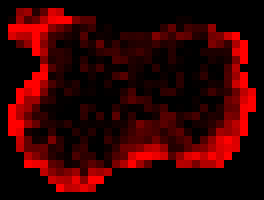
Proposed LADMM
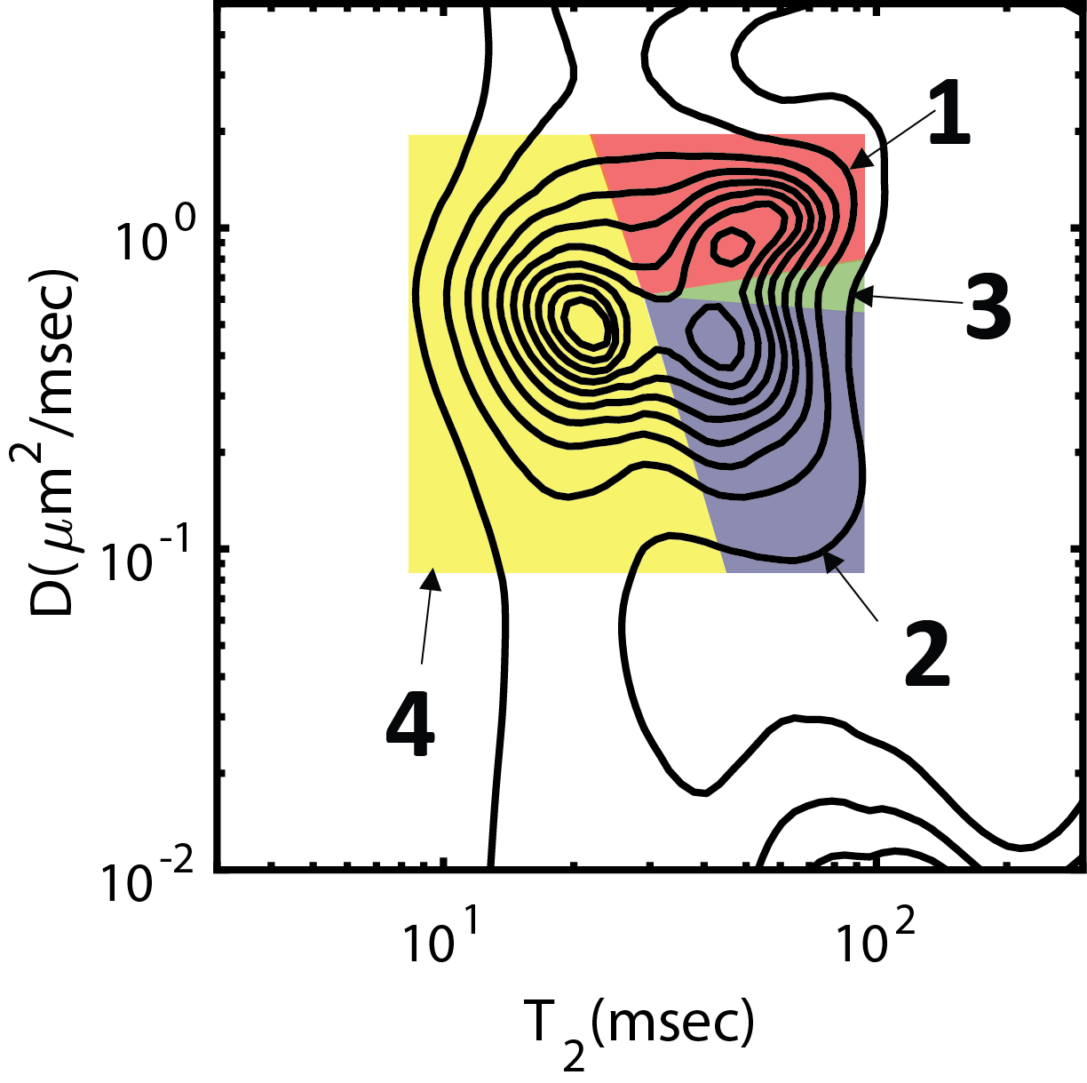
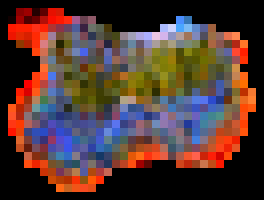
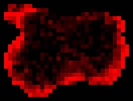
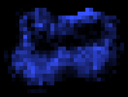
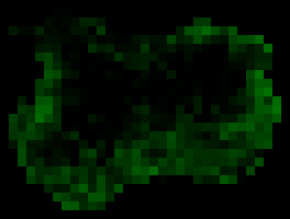
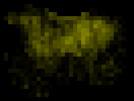
Lawson-Hanson

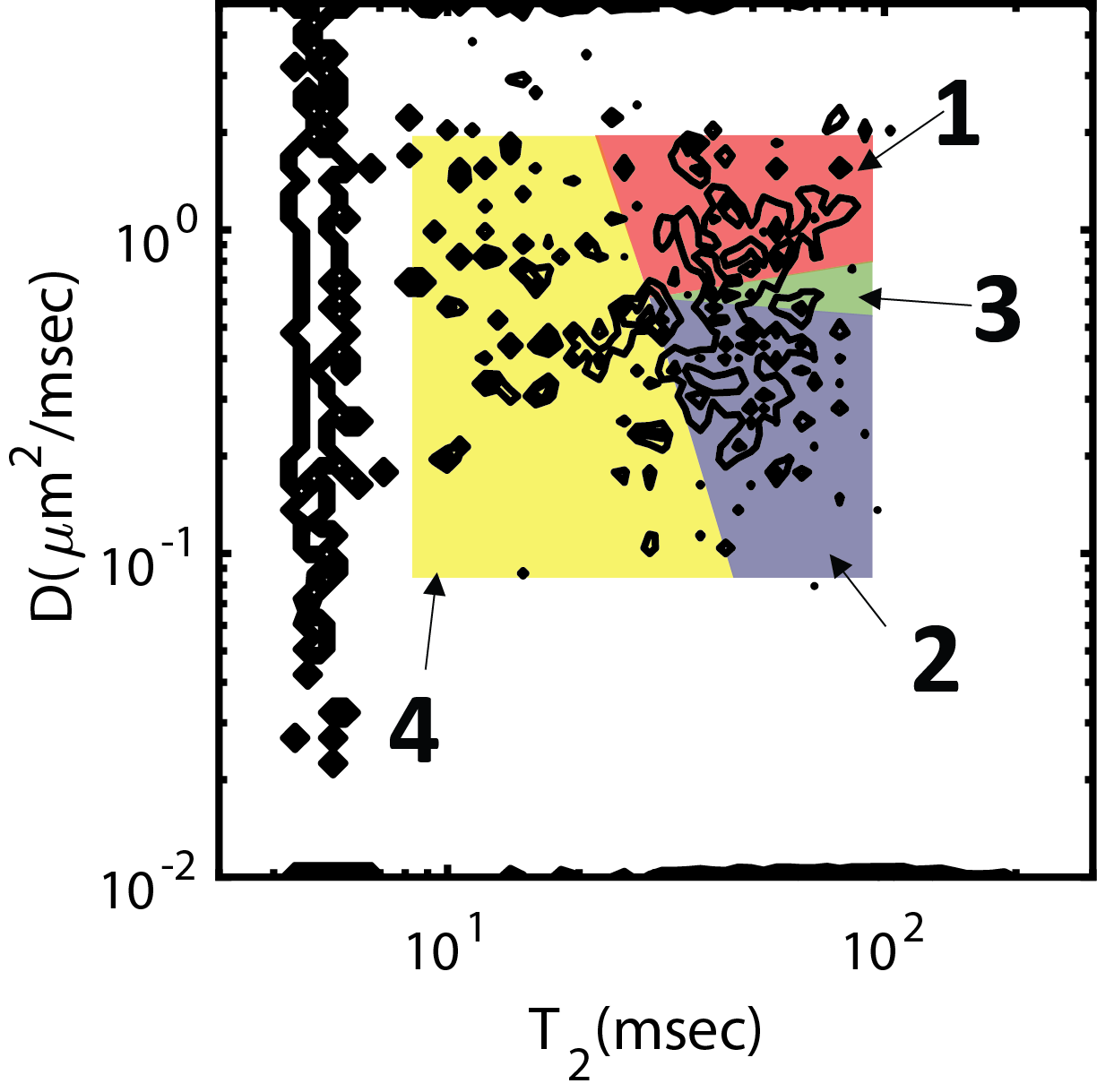
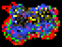
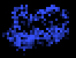
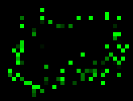
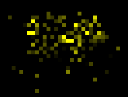
Figure 1: Component maps and spatially-averaged diffusion-relaxation spectra obtained for the DR-CSI data using ADMM, LADMM, and the voxel-by-voxel approach using the Lawson-Hanson algorithm. The component maps were obtained by spectrally-integrating different regions of the 2D diffusion-relaxation spectrum as indicated in the spatially-averaged spectra.

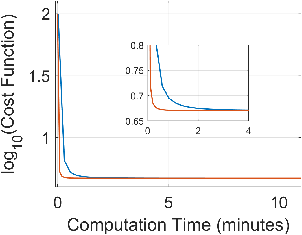
(a)

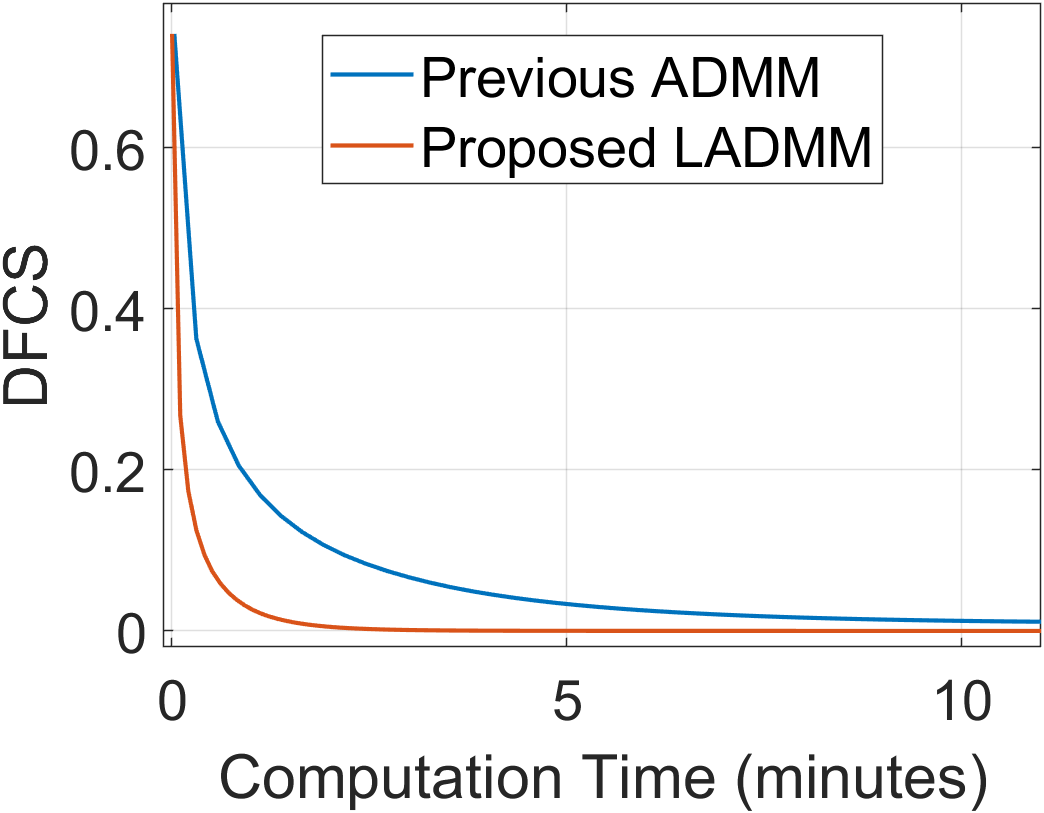
(b)

Figure 2: Convergence of ADMM and LADMM for DR-CSI.

IV Results

We compared our new LADMM algorithm against the previous ADMM algorithm [1] in a range of different scenarios. To evaluate convergence, we tracked the cost function value and the distance from the converged solution (DFCS) as a function of computation time, with DFCS defined as

$$\text{DFCS}(\mathbf{f}^{k})\triangleq\frac{\|\mathbf{f}^{k}-\mathbf{f}^{*}\|_{2}}{\|\mathbf{f}^{*}\|_{2}}$$ (33)

where $\mathbf{f}^{k}$ and $\mathbf{f}^{*}$ are respectively the estimates of the spectroscopic image obtained at iteration $k$ and after the final convergence of LADMM. (Note that the ill-posedness of the problem means that many different solutions will have similar cost function values, such that the cost function alone provides limited information about the convergence of $\mathbf{f}^{k}$). Computation times were measured in MATLAB.

The following subsections report results from four datasets from a range of different application scenarios.

IV-A DR-CSI

We evaluated LADMM on one of the diffusion-$T_{2}$ DR-CSI datasets from Ref. [1], corresponding to an ex vivo injured mouse spinal cord (specifically, the dataset described in Ref. [1] as “injured subject 1”). The details of this dataset and problem formulation were described in detail in Ref. [1], but some of the key parameters of the optimization problem were that data acquisition involved $P=28$ diffusion-relaxation encodings, the dictionary had $Q=4900$ elements, and the 2D image had $N=825$ voxels. The resulting 4D spectroscopic image was comprised of a 2D diffusion-$T_{2}$ spectrum of size 70$\times$70 at each spatial image location.

Fig. 1 shows component maps and spatially-averaged diffusion-relaxation spectra obtained by both ADMM and LADMM in this case, while Fig. 2 compares their convergence characteristics. As expected, the ADMM and LADMM component maps closely matched one another (and also match the spectra and component maps from Ref. [1], which contains a more detailed interpretation of these results), demonstrating that the two algorithms yield similar results. Notably, LADMM converges much faster than ADMM (while this is true for both the cost function value and the DFCS, the cost function values in Fig. 2 appear to converge much faster than the DFCS – this is not surprising given the ill-posed nature of the inverse problem, and our subsequent analysis will focus on DFCS). For example, the DFCS value obtained by ADMM after 10 minutes of computation was achieved by LADMM in only 1.4 minutes (roughly a $7.0\times$ improvement).

For reference, Fig. 1 also shows an example of the results obtained from voxel-by-voxel spectrum estimation using the Lawson-Hanson algorithm (see Sec. II-B). Although the voxel-by-voxel estimation results can be obtained very quickly (roughly 15 seconds of computation time) relative to spatially-regularized reconstruction, it is clear that the resulting spectra and spatial component maps qualitatively appear to be quite noisy, with less spectral coherence and less spatial correspondence with known anatomy.

IV-B Inversion-Recovery Multi-Echo Spin-Echo RR-CSI

We also evaluated LADMM on one of the IR-MSE $T_{1}$-$T_{2}$ RR-CSI datasets from Ref. [2] of the human brain (specifically, the dataset described in Ref. [2] as “subject 1”). The details of this dataset and problem formulation were described in detail in Ref. [2], but some of the key parameters of the optimization problem were that data acquisition involved $P=105$ $T_{1}$-$T_{2}$ relaxation encodings, the dictionary had $Q=10000$ elements, and the 2D image had $N=6150$ voxels. The resulting 4D spectroscopic image was comprised of a 2D $T_{2}$-$T_{2}$ spectrum of size 100$\times$100 at each spatial image location.

Fig. 3 shows component maps obtained in this case for LADMM, which were closely matched to the ADMM results (not shown due to space constraints, although spatial maps and $T_{1}$-$T_{2}$ spectra for ADMM were shown and discussed in detail in Ref. [2]). Fig. 4 compares the convergence characteristics of ADMM and LADMM for this case. where we still observe that the DFCS for LADMM converges much faster than ADMM. For example, the DFCS value obtained by ADMM after 10 hours of computation was achieved by LADMM in only 1.8 hours (roughly a $5.7\times$ improvement). Note that this problem size is larger than it was in the previous DR-CSI case, and the computation times are also longer.

	Composite	Comp. 1	Comp. 2	Comp. 3	Comp. 4	Comp. 5	Comp. 6
LADMM

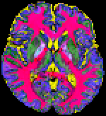
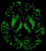
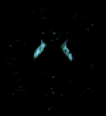
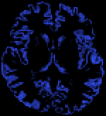
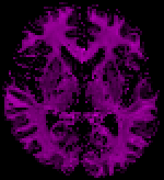
Figure 3: Component maps obtained for the RR-CSI data using LADMM. The component maps were obtained by spectrally-integrating different regions of the 2D $T_{1}$-$T_{2}$ spectrum as described in Ref. [2].

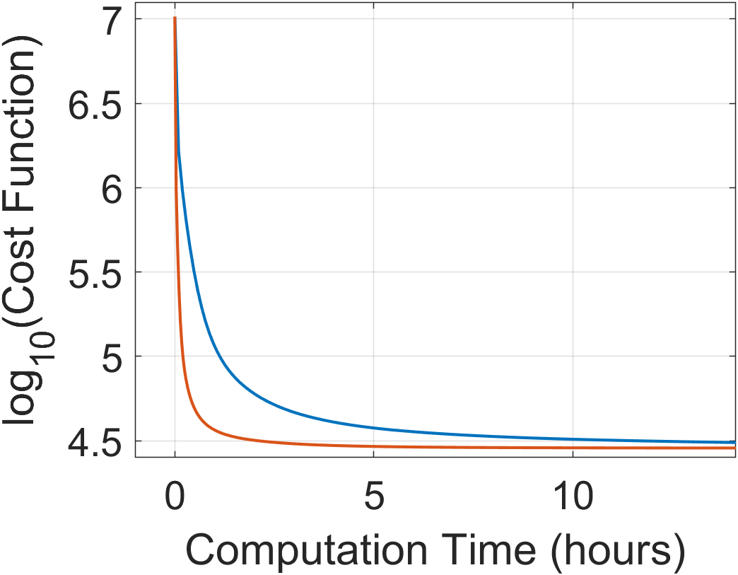
(a)

(b)

Figure 4: Convergence of ADMM and LADMM for RR-CSI.

IV-C Multi-Echo Spin Echo $T_{2}$ Relaxometry

The previous subsections demonstrated that LADMM could substantially accelerate computations in high-dimensional problems, where a 2D spectrum was estimated at every spatial location. In this subsection, we evaluate a lower-dimensional problem where we desire to estimate a 1D $T_{2}$-relaxation spectrum from a series of multi-echo spin-echo data, while still using spatial regularization to improve the estimation results. Specifically, we considered the multicomponent $T_{2}$ dataset in vivo human brain described in Fig. 11 of Ref. [2], where data acquisition involved $P=32$ $T_{2}$ encodings, the dictionary had $Q=300$ elements, and there were $N=6160$ voxels. The resulting 3D spectroscopic image was comprised of a 1D $T_{2}$ spectrum of size 300 at each spatial image location.

Fig. 5 shows component maps obtained in this case for LADMM, which were closely matched to the ADMM results (not shown due to space constraints, although spatial maps and $T_{2}$ spectra for ADMM were shown and discussed in detail in Ref. [2]). Notably, this type of 1D relaxometry experiment is less powerful than the 2D relaxometry experiment described in the previous subsection, as can be seen from the fact only 3 components are successfully resolved in this case, as compared to 6 components for RR-CSI. However, the 1D experiment has the benefit of requiring a much shorter acquisition than a 2D experiment, while also requiring less computational effort.

Fig. 6 compares the convergence characteristics of ADMM and LADMM for this case, where we again observe that the DFCS for LADMM converges much faster than ADMM. The DFCS value obtained by ADMM after 1 hour of computation was achieved by LADMM in only 11 minutes (roughly a $5.6\times$ improvement).

Composite	Comp. 1	Comp. 2	Comp. 3

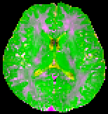
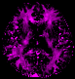
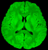
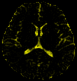
Figure 5: Component maps obtained for $T_{2}$ relaxometry data using LADMM. The component maps were obtained by spectrally-integrating different regions of the 1D $T_{2}$ spectrum as described in Ref. [2].

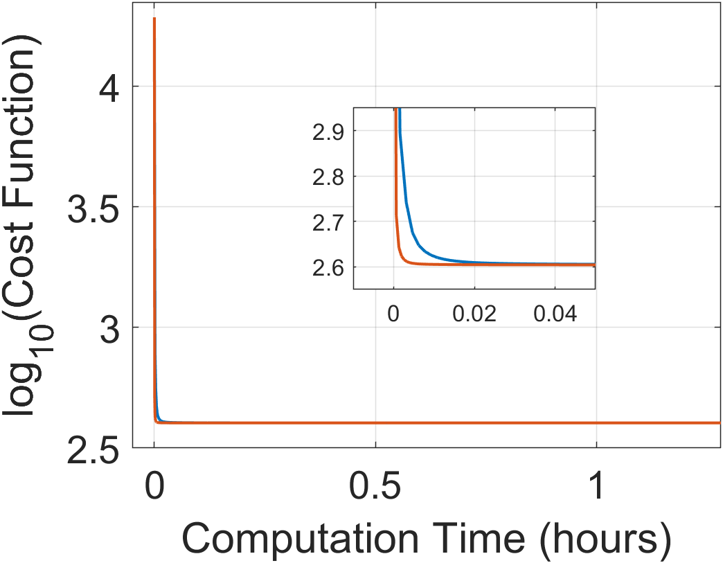
(a)

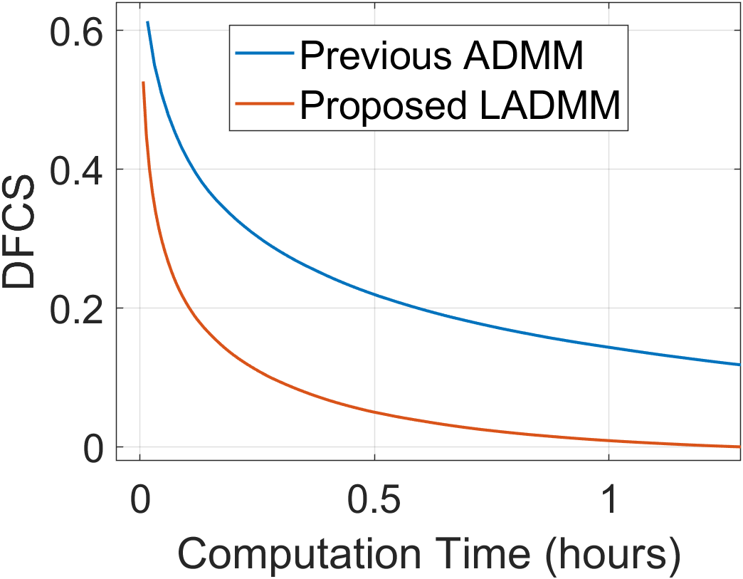
(b)

Figure 6: Convergence of ADMM and LADMM for $T_{2}$ relaxometry.

Composite	Comp. 1	Comp. 2	Comp. 3	Comp. 4	Comp. 5	Comp. 6

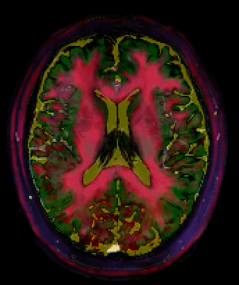
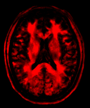
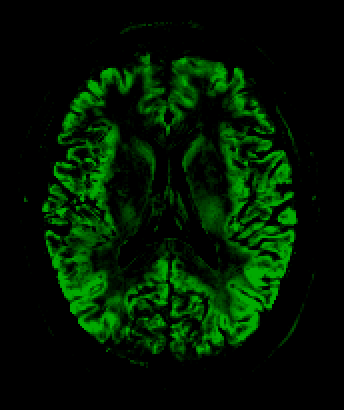
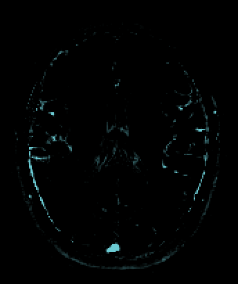
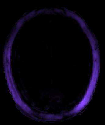
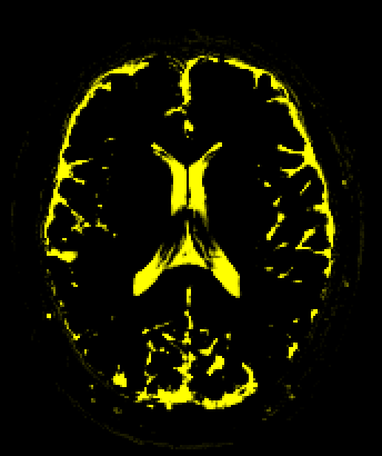
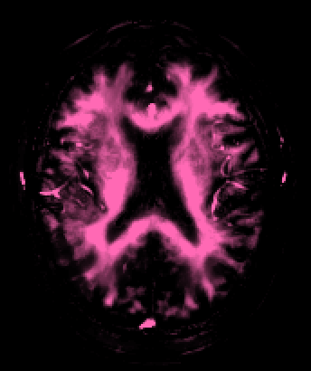
Figure 7: Component maps obtained for MRF data using LADMM.

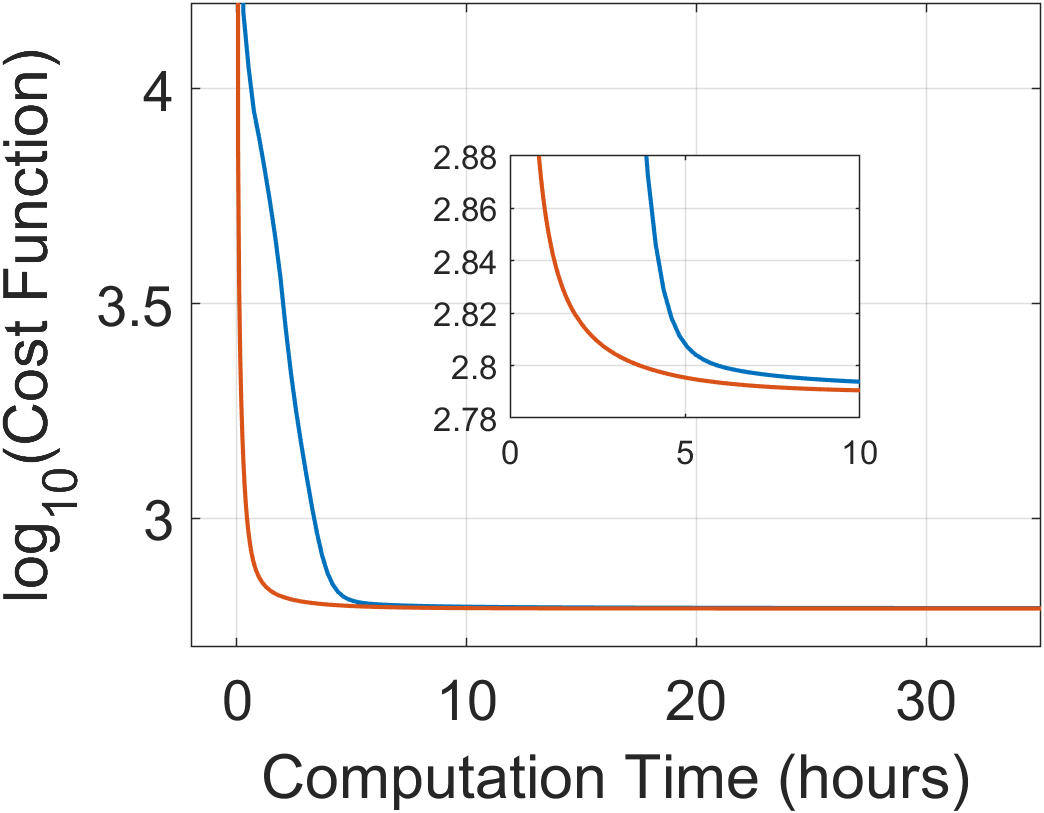
(a)

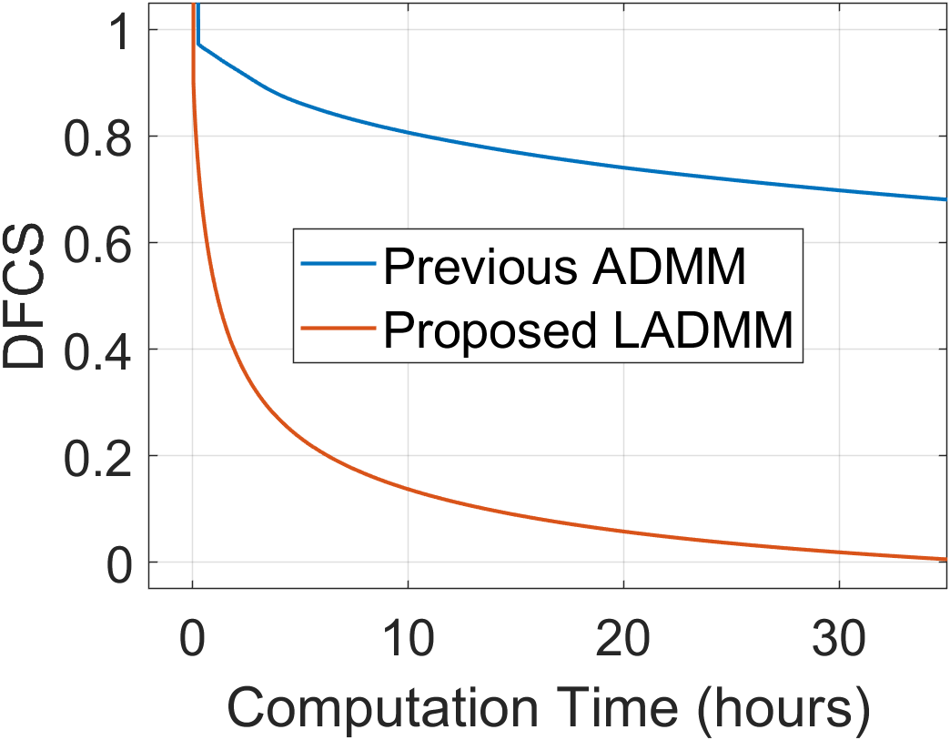
(b)

Figure 8: Convergence of ADMM and LADMM for MRF.

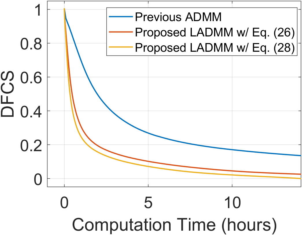
Figure 9: Convergence of LADMM using full-rank matrices (Eq. (26)) versus low-rank matrix approximations (Eq. (28)).

IV-D MR Fingerprinting RR-CSI

As a final test case, we considered estimation of $T_{1}$-$T_{2}$ spectroscopic images from data acquired using an MRF acquisition with a ViSTa preparation block to emphasize short $T_{1}$ components such as myelin water [33, 48]. A 2D slice of the in vivo human brain was acquired without acceleration ($32$ spiral interleaves to cover k-space at the Nyquist rate) with $1$ mm in-plane spatial resolution and $10$ mm slice thickness using a $3$T Siemens Prisma scanner. A total of $P=540$ contrast-encoded images were acquired with varying sequence parameters. To account for $B_{1}$ (flip angle) inhomogeneity, we acquired a $B_{1}$ map which was quantized to 13 different levels (uniformly spaced from 0.7-1.3, where a value of 1.0 indicates a nominal flip angle). Dictionaries were constructed using extended phase graph simulations for $(T_{1},T_{2})$ parameter combinations corresponding to every possible combination of 101 different $T_{1}$ values (ranging from 100-3000 msec, spaced logarithmically) with 101 different $T_{2}$ values (ranging from 1-300 msec, spaced logarithmically) for each of the $B_{1}$ values ($Q=10201$), and different dictionaries were used for different spatial locations based on the $B_{1}$ map. The resulting 4D spectroscopic image was comprised of a 2D $T_{2}$-$T_{2}$ spectrum of size 101$\times$101 at each of $N=35260$ spatial locations.

Fig. 7 shows component maps for obtained using LADMM for this case, where we were successfully able to resolve 6 anatomically plausible tissue components. ADMM results were similar and not shown. Fig. 8 compares convergence characteristics, where we again observe that the DFCS for LADMM converged substantially faster than for ADMM. For example, the DFCS value obtained for ADMM after 30 hours was obtained by LADMM after only 22 minutes (roughly an 81.1$\times$ improvement).

V Discussion

The results in the previous section demonstrated that the new LADMM algorithm offers substantial advantages compared to the previous ADMM algorithm across a range of different problems. While these improvements were primarily due to the problem simplifications offered by LADMM, the ability to use low-rank approximation (Eq. (28)) also contributed to computational efficiency. The benefits of low-rank approximation are illustrated for the RR-CSI data in Fig. 9, where we observe that the use of low-rank approximation yields a small improvement in computation speed.

An interesting feature of our LADMM approach is that the $\mathbf{f}$-subproblem is easily parallelized across different spatial locations, while the $\mathbf{z}$-subproblem is easily parallelized across different spectral positions. This suggests that the proposed LADMM approach could be further accelerated in a parallel computing environment – we did not explore that approach here, although it is an interest direction for future research.

In this work, we applied LADMM to solve an ill-posed inverse problem with nonnegativity constraints, quadratic data-fidelity constraints, and a quadratic spatial-roughness penalty. However, the principles we used in this scenario are quite general, and we anticipate that similar approaches may prove useful across a wide range of different optimization problems with similar structure.

VI Conclusion

We proposed and evaluated an efficient algorithm, based on LADMM, for spatially-regularized partial volume component mapping from high-dimensional multiparametric MRI data. The proposed approach was demonstrated to enable substantial computational improvements (ranging between roughly 5$\times$-80$\times$ acceleration for the cases we tried) across a range of different scenarios. We expect that this reduction in computational complexity will make it easier for the community to access the substantial benefits offered by spatial regularization in these kinds of problem settings.

References

- [1] D. Kim, E. K. Doyle, J. L. Wisnowski, J. H. Kim, and J. P. Haldar, “Diffusion-relaxation correlation spectroscopic imaging: A multidimensional approach for probing microstructure,” Magn. Reson. Med., vol. 78, pp. 2236–2249, 2017.
- [2] D. Kim, J. L. Wisnowski, C. T. Nguyen, and J. P. Haldar, “Multidimensional correlation spectroscopic imaging of exponential decays: From theoretical principles to in vivo human applications,” NMR Biomed., vol. 33, p. e4244, 2020.
- [3] D. McGivney, A. Deshmane, Y. Jiang, D. Ma, C. Badve, A. Sloan, V. Gulani, and M. Griswold, “Bayesian estimation of multicomponent relaxation parameters in magnetic resonance fingerprinting,” Magn. Reson. Med., vol. 80, pp. 159–170, 2018.
- [4] A. Deshmane, D. F. McGivney, D. Ma, Y. Jiang, C. Badve, V. Gulani, N. Seiberlich, and M. A. Griswold, “Partial volume mapping using magnetic resonance fingerprinting,” NMR Biomed., vol. 32, p. e4082, 2019.
- [5] S. Tang, C. Fernandez-Granda, S. Lannuzel, B. Bernstein, R. Lattanzi, M. Cloos, F. Knoll, and J. Asslander, “Multicompartment magnetic resonance fingerprinting,” Inverse Probl., vol. 34, p. 094005, 2018.
- [6] M. Nagtegaal, P. Koken, T. Amthor, and M. Doneva, “Fast multi-component analysis using a joint sparsity constraint for MR fingerprinting,” Magn. Reson. Med., vol. 83, pp. 521–534, 2020.
- [7] P. J. Slator, M. Palombo, K. Miller, C. F. Westin, F. Laun, D. Kim, J. P. Haldar, D. Benjamini, G. Lemberskiy, J. P. de Almeida Martins, and J. Hutter, “Combined diffusion-relaxometry microstructure imaging: Current status and future prospects,” Magn. Reson. Med., vol. 86, pp. 2987–3011, 2021.
- [8] D. Benjamini and P. J. Basser, “Multidimensional correlation MRI,” NMR Biomed., vol. 33, p. e4226, 2020.
- [9] F. O’Sullivan, “Imaging radiotracer model parameters in PET: A mixture analysis approach,” IEEE Trans. Med. Imaging, vol. 12, pp. 399–412, 1993.
- [10] M. Ingrisch and S. Sourbron, “Tracer-kinetic modeling of dynamic contrast-enhanced MRI and CT: A primer,” J. Pharmacokinet. Pharmacodyn., vol. 40, pp. 281–300, 2013.
- [11] M. D. Does, “Inferring brain tissue composition and microstructure via MR relaxometry,” NeuroImage, vol. 182, pp. 136–148, 2018.
- [12] D. C. Alexander, T. B. Dyrby, M. Nilsson, and H. Zhang, “Imaging brain microstructure with diffusion MRI: Practicality and applications,” NMR Biomed., vol. 32, p. e3841, 2019.
- [13] A. A. Istratov and O. F. Vyvenko, “Exponential analysis in physical phenomena,” Rev. Sci. Instrum., vol. 70, pp. 1233–1257, 1999.
- [14] H. Celik, M. Bouhrara, D. A. Reiter, K. W. Fishbein, and R. G. Spencer, “Stabilization of the inverse Laplace transform of multiexponential decay through introduction of a second dimension,” J. Magn. Reson., vol. 236, pp. 134–139, 2013.
- [15] R. M. Kroeker and R. M. Henkelman, “Analysis of biological NMR relaxation data with continuous distributions of relaxation times,” J. Magn. Reson., vol. 69, pp. 218–235, 1986.
- [16] K. P. Whittall and A. L. MacKay, “Quantitative interpretation of NMR relaxation data,” J. Magn. Reson., vol. 84, pp. 134–152, 1989.
- [17] L. Venkataramanan, Y.-Q. Song, and M. D. Hurlimann, “Solving Fredholm integrals of the first kind with tensor product structure in 2 and 2.5 dimensions,” IEEEE Trans. Signal Process., vol. 50, pp. 1017–1026, 2002.
- [18] R. Bai, A. Cloninger, W. Czaja, and P. J. Basser, “Efficient 2D MRI relaxometry using compressed sensing,” J. Magn. Reson., vol. 255, pp. 88–99, 2015.
- [19] D. Benjamini and P. J. Basser, “Use of marginal distributions constrained optimization (MADCO) for accelerated 2D MRI relaxometry and diffusometry,” J. Magn. Reson., vol. 271, pp. 40–45, 2016.
- [20] Y. Lin, J. P. Haldar, Q. Li, P. S. Conti, and R. M. Leahy, “Sparsity constrained mixture modeling for the estimation of kinetic parameters in dynamic PET,” IEEE Trans. Med. Imaging, vol. 33, pp. 173–185, 2014.
- [21] D. Hwang and Y. P. Du, “Improved myelin water quantification using spatially regularized non-negative least squares algorithm,” J. Magn. Reson. Imaging, vol. 30, pp. 203–208, 2009.
- [22] D. Kumar, T. D. Nguyen, S. A. Gauthier, and A. Raj, “Bayesian algorithm using spatial priors for multiexponential T2 relaxometry from multiecho spin echo MRI,” Magn. Reson. Med., vol. 68, pp. 1536–1543, 2012.
- [23] C. Labadie, J.-H. Lee, W. D. Rooney, S. Jarchow, M. Aubert-Frecon, C. S. Springer, Jr, and H. E. Moller, “Myelin water mapping by spatially regularized longitudinal relaxographic imaging at high magnetic fields,” Magn. Reson. Med., vol. 71, pp. 375–387, 2014.
- [24] D. Kumar, H. Hariharan, T. D. Faizy, P. Borchert, S. Siemonsen, J. Fiehler, R. Reddy, and J. Sedlacik, “Using 3D spatial correlations to improve the noise robustness of multi component analysis of 3D multi echo quantitative T2 relaxometry data,” NeuroImage, vol. 178, pp. 583–601, 2018.
- [25] M. Zimmermann, A.-M. Oros-Peusquens, E. Iordanishvili, S. Shin, S. D. Yun, Z. Abbas, and N. J. Shah, “Multi-exponential relaxometry using -regularized iterative NNLS (MERLIN) with application to myelin water fraction imaging,” IEEE Trans. Med. Imaging, vol. 38, pp. 2676–2686, 2019.
- [26] S. Boyd, N. Parikh, E. Chu, B. Peleato, and J. Eckstein, “Distributed optimization and statistical learning via the alternating direction method of multipliers,” Found. Trends Mach. Learn., vol. 3, pp. 1–122, 2011.
- [27] B. He, L.-Z. Liao, D. Han, and H. Yang, “A new inexact alternating directions method for monotone variational inequalities,” Math. Program., vol. 92, pp. 103–118, 2002.
- [28] X. Zhang, M. Burger, and S. Osher, “A unified primal-dual algorithm framework based on Bregman iteration,” J. Sci. Comput., vol. 46, pp. 20–46, 2011.
- [29] B. He, F. Ma, and X. Yuan, “Optimally linearizing the alternating direction method of multipliers for convex programming,” Comput. Optim. Appl., vol. 75, pp. 361–388, 2020.
- [30] M. Fazel, T. K. Pong, D. Sun, and P. Tseng, “Hankel matrix rank minimization with applications to system identification and realization,” SIAM J. Matrix Anal. Appl., vol. 34, pp. 946–977, 2013.
- [31] M. Tao, “Convergence study of indefinite proximal ADMM with a relaxation factor,” Comput. Optim. Appl., vol. 77, pp. 91–123, 2020.
- [32] W. Deng and W. Yin, “On the global and linear convergence of the generalized alternating direction method of multipliers,” J. Sci. Comput., vol. 66, pp. 889–916, 2016.
- [33] Y. Liu, C. Liao, D. Kim, K. Setsompop, and J. P. Haldar, “Estimating multicomponent 2D relaxation spectra with a ViSTa-MR fingerprinting acquisition,” in Proc. ISMRM, 2022, p. 4389.
- [34] D. Kim, B. Zhao, L. L. Wald, and J. P. Haldar, “Multidimensional T1 relaxation-T2 relaxation correlation spectroscopic imaging witha magnetic resonance fingerprinting acquisition,” in Proc. ISMRM, 2019, p. 4991.
- [35] S. W. Provencher, “A constrained regularization method for inverting data represented by linear algebraic or integral equations,” Comput. Phys. Commun., vol. 27, pp. 213–227, 1982.
- [36] D. Varadarajan and J. P. Haldar, “A majorize-minimize framework for Rician and non-central chi MR images,” IEEE Trans. Med. Imaging, vol. 34, pp. 2191–2202, 2015.
- [37] S. Boyd, Convex Optimization. Cambridge: Cambridge University Press, 2004.
- [38] M. Slawski and M. Hein, “Non-negative least squares for high-dimensional linear models: Consistency and sparse recovery without regularization,” Electronic J. Statist., vol. 7, pp. 3004–3056, 2013.
- [39] C. L. Lawson and R. J. Hanson, Solving Least Squares Problems. Philadelphia: SIAM, 1995.
- [40] M. V. Afonso, J. M. Bioucas-Dias, and M. A. T. Figueiredo, “An augmented Langrangian approach to the constrained optimization formulation of imaging inverse problems,” IEEE Trans. Image Process., vol. 20, pp. 681–695, 2011.
- [41] P. L. Combettes and J.-C. Pesquet, “Proximal splitting methods in signal processing,” in Fixed-Point Algorithms for Inverse Problems in Science and Engineering, H. H. Bauschke, R. S. Burachik, P. L. Combettes, V. Elser, D. R. Luke, and H. Wolkowicz, Eds. New York: Springer New York, 2011, pp. 185–212.
- [42] N. Parikh and S. Boyd, “Proximal algorithms,” Found. Trends Optim., vol. 1, pp. 127–239, 2014.
- [43] A. Beck, First-Order Methods in Optimization. Philadelphia: SIAM, 2017.
- [44] M. Yang, D. Ma, Y. Jiang, J. Hamilton, N. Seiberlich, M. A. Griswold, and D. McGivney, “Low rank approximation methods for MR fingerprinting with large scale dictionaries,” Magn. Reson. Med., vol. 79, pp. 2392–2400, 2018.
- [45] E. Ghadimi, A. Teixeira, I. Shames, and M. Johansson, “Optimal parameter selection for the alternating direction method of multipliers (ADMM): Quadratic problems,” IEEE Trans. Automat. Contr., vol. 60, pp. 644–658, 2015.
- [46] B. S. He, H. Yang, and S. L. Wang, “Alternating direction method with self-adaptive penalty parameters for monotone variational inequalities,” J. Optim. Theory Appl., vol. 106, pp. 337–356, 2000.
- [47] Z. Xu, M. Figueiredo, and T. Goldstein, “Adaptive ADMM with Spectral Penalty Parameter Selection,” in Proc. AISTATS, 2017, pp. 718–727.
- [48] C. Liao, X. Cao, S. S. Iyer, S. Schauman, Z. Zhou, X. Yan, Q. Chen, Z. Li, N. Wang, T. Gong, Z. Wu, H. He, J. Zhong, Y. Yang, A. Kerr, K. Grill-Spector, and K. Setsompop, “High-resolution myelin-water fraction and quantitative relaxation mapping using 3D ViSTa-MR fingerprinting,” Magn. Reson. Med., 2024, In Press.