MAPPING: Debiasing Graph Neural Networks for Fair Node Classification with Limited Sensitive Information Leakage

Abstract.

Despite remarkable success in diverse web-based applications, Graph Neural Networks(GNNs) inherit and further exacerbate historical discrimination and social stereotypes, which critically hinder their deployments in high-stake domains such as online clinical diagnosis, financial crediting, etc. However, current fairness research that primarily craft on i.i.d data, cannot be trivially replicated to non-i.i.d. graph structures with topological dependence among samples. Existing fair graph learning typically favors pairwise constraints to achieve fairness but fails to cast off dimensional limitations and generalize them into multiple sensitive attributes; besides, most studies focus on in-processing techniques to enforce and calibrate fairness, constructing a model-agnostic debiasing GNN framework at the pre-processing stage to prevent downstream misuses and improve training reliability is still largely under-explored. Furthermore, previous work on GNNs tend to enhance either fairness or privacy individually but few probe into their interplays. In this paper, we propose a novel model-agnostic debiasing framework named MAPPING (Masking And Pruning and Message-Passing trainING) for fair node classification, in which we adopt the distance covariance($dCov$)-based fairness constraints to simultaneously reduce feature and topology biases in arbitrary dimensions, and combine them with adversarial debiasing to confine the risks of attribute inference attacks. Experiments on real-world datasets with different GNN variants demonstrate the effectiveness and flexibility of MAPPING. Our results show that MAPPING can achieve better trade-offs between utility and fairness, and mitigate privacy risks of sensitive information leakage.

1. Introduction

Graph Neural Networks (GNNs) have shown superior performance in various web applications, including recommendation systems(Fan et al., 2019) and online advertisement(Yang et al., 2022). Message-passing schemes(MP)(Wu et al., 2020) empower GNNs by aggregating node information from local neighborhoods, thereby rendering the clearer boundary between similar and dissimilar nodes(Rahman et al., 2019) to facilitate downstream graph tasks. However, disparities among different demographic groups can be perpetuated and amplified, causing severe social consequences in high-stake scenarios(Suresh and Guttag, 2021). For instance, in clinical diagnosis(Hamberg, 2008), men are more extensively treated than women with the same severity of symptoms in a plethora of diseases, and older men aged 50 years or above receive extra healthcare or life-saving interventions than older women. With more GNNs adopted in medical analysis, gender discrimination may further deteriorate and directly cause misdiagnosis for women or even life endangerment.

Unfortunately, effective bias mitigation on non-i.i.d graphs is still largely under-explored, which particularly faces the following two problems: first, they tend to employ in-processing methods(Dai and Wang, 2021; Agarwal et al., 2021; Oneto et al., 2020; Jiang et al., 2022), while few work jointly alleviate feature and topology biases at the pre-processing stage and then feed debiased data into any GNN variants. For instance, FairDrop(Spinelli et al., 2021) pre-modifies graph topologies to minimize distances among sensitive subgroups. However, it ignores the significant roles of node features to encode biases. Kamiran et al.(Kamiran and Calders, 2011) and Wang et al.(Wang et al., 2019) pre-debias features by ruffling, reweighting, or counterfactual perturbation, whereas their methods cannot be trivially applied on GNNs since unbiased features with biased topologies can result in biased distributions among different groups(Dong et al., 5555). Second, although recent studies(Dong et al., 2022) fill the above gap, they introduce pairwise constraints, e.g., covariance($Cov$), mutual information($MI$), Wasserstein distance($Was$)(Villani, 2003), to promote fairness, which, nonetheless, are computationally inefficient in high dimensions and cannot be easily extended into multiple sensitive attributes. Besides, $Cov$ cannot reveal mutual independence between target variables and sensitive attributes; $MI$ cannot break dimensional limitations and be intractable to compute, and some popular estimators, e.g., MINE(Belghazi et al., 2018) are proved to be heavily biased(Song and Ermon, 2020); and Was is sensitive to outliers(Staerman et al., 2021), which hinders its uses in heavy-tailed data samples. To tackle these issues, we adopt a distribution-free, scale-invariant(Székely et al., 2007) and outlier-resistant(Hou et al., 2022) metric - $dCov$ as fairness constraints, which most importantly, allows computations in arbitrary dimensions and can guarantee independence. We combine it with adversarial training to develop a feature and topology debiasing framework for GNNs.

Sensitive attributes not only result in bias aggravation but also raise data privacy concerns. Prior work elucidate that GNNs are vulnerable to attribute inference attacks(Duddu et al., 2020). Even though such identifiable information is masked and then released in public by data owners for specific purposes, e.g., research institutions publish pre-processed real-world datasets for researchers to use, malicious third-parties can combine masked features with prior knowledge to recover them. Meanwhile, links are preferentially connected w.r.t. sensitive attributes in reality, therefore, topological structures can contribute to sensitive membership identification. More practically, some data samples, e.g., users or customers, may unintentionally disclose their sensitive information to the public. Attackers can exploit these open resources to launch attribute inference attacks, which further amplify group inequalities and bring immeasurable social impacts. Thus, it is imperative to confine such privacy risks derived from features and topologies at the pre-processing stage.

Prior privacy-preserving studies mainly deploy in-processing techniques, such as attack-and-defense games(Li et al., 2020; Liao et al., 2021) and/or resort to privacy constraints(Hu et al., 2022; Wang et al., 2021; Liao et al., 2021) to fight against potential privacy risks on GNNs. However, these methods are not designed for multiple sensitive attributes, and their constraints, e.g., $Cov$ or $MI$, have deficiencies as previously described. Most importantly, they fail to consider fairness issues. PPFR(Zhang et al., 2023) is the first work to explore such interactions on GNNs, which empirically proves that the risks of link-stealing attacks increase as individual fairness is boosted with limited utility costs, but it centers on post-processing techniques to achieve individual fairness. Yet this work motivates us to explore whether fairness enhancements can simultaneously reduce privacy risks. To address the above issues, we propose MAPPING with $dCov$-based constraints and adversarial training to decorrelate sensitive information from features and topologies, which aligns with the same goal of fair learning. We evaluate the privacy risks via attribute inference attacks and the empirical results show that MAPPING successfully guarantees fairness while ameliorating sensitive information leakage. To the best of our knowledge, this is the first work to highlight the alignments between group-level fairness and multiple sensitive attribute privacy on GNNs at the pre-processing stage. In summary, our main contributions are threefold:

MAPPING We propose a novel debiasing framework called MAPPING for fair node classification, which confines sensitive attribute inferences from pre-debiased features and topologies. Our empirical results demonstrate that MAPPING obtains better flexibility and generalization to any GNN variants.

Effectiveness and Efficiency We evaluate MAPPING on three real-world datasets and compare MAPPING with vanilla GNNs and state-of-the-art debiasing models. The experimental results confirm the effectiveness and efficiency of MAPPING.

Alignments and Trade-offs We discuss the alignments between fairness and privacy on GNNs, and illustrate MAPPING can achieve better trade-offs between utility and fairness while mitigate the privacy risks of attribute inference.

2. Preliminaries

In this section, we present the notations and introduce preliminaries of GNNs, $dCov$, two fairness metrics $\Delta SP$ and $\Delta EO$, and attribute inference attacks to measure sensitive information leakage.

2.1. Notations

In our work, we focus on node classification tasks. Given an undirected attributed graph $\mathcal{G}=\left(\mathcal{V},\mathcal{E},\mathcal{X}\right)$, where $\mathcal{V}$ denotes a set of nodes, $\mathcal{E}$ denotes a set of edges and the node feature set $\mathcal{X}=\left(\mathcal{X}_{N},S\right)$ concatenates non-sensitive features $\mathcal{X}_{N}\in\mathcal{R}^{n\times d}$ and a sensitive attribute $S$. The goal of node classification is to predict the ground-truth labels $\mathcal{Y}$ as $\hat{Y}$ after optimizing the objective function $f_{\theta}(\mathcal{Y},\hat{Y})$. Beyond the above notations, $A\in\mathbb{R}^{n\times n}$ is the adjacency matrix, where $n=|\mathcal{V}|$, $A_{ij}=1$ if two nodes $\left(v_{i},v_{j}\right)\in\mathcal{E}$, otherwise, $A_{ij}=0$.

2.2. Graph Neural Networks

GNNs utilize MP to aggregate information of each node $v\in\mathcal{V}$ from its local neighborhood $\mathcal{N}(v)$ and thereby update its representation $H_{v}^{l}$ at layer $l$, which can be expressed as:

(1) $$H_{v}^{l}=UPD^{l}(H_{v}^{l-1},AGG^{l-1}(\{H_{u}^{l-1}:u\in\mathcal{N}(v)\}))$$

where $H_{v}^{0}=X_{v}$, and $UPD$ and $AGG$ are arbitrary differentiable functions that distinguish the different GNN variants. For a $l$-th layer GNN, typically, $H_{v}^{l}$ is fed into i.e., a linear classifier with a softmax function to predict node $v$’s label.

2.3. Distance Covariance

$dCov$ reveals independence between two random variables $X\in\mathbb{R}^{p}$ and $Y\in\mathbb{R}^{q}$ that follow any distribution, where $p$ and $q$ are arbitrary dimensions. As defined in (Székely et al., 2007), given a sample $(X,Y)=\{(X_{k},Y_{k}):k=1,\dots,n\}$ from a joint distribution, the empirical $dCov$ - $\mathcal{V}_{n}^{2}(X,Y)$ and its corresponding distance correlation($dCor$) - $\mathcal{R}_{n}^{2}(X,Y)$ are defined as:

(2) $$\mathcal{V}_{n}^{2}(X,Y)=\frac{1}{n^{2}}\sum_{k,l=1}^{n}A_{kl}B_{kl}$$

$$\mathcal{R}_{n}^{2}(X,Y)=\begin{cases}\frac{\mathcal{V}_{n}^{2}(X,Y)}{\sqrt{\mathcal{V}_{n}^{2}(X)\mathcal{V}_{n}^{2}(Y)}},&\mathcal{V}_{n}^{2}(X)\mathcal{V}_{n}^{2}(Y)>0\\ 0,&\mathcal{V}_{n}^{2}(X)\mathcal{V}_{n}^{2}(Y)=0\end{cases}$$

where $A_{kl}=a_{kl}-\bar{a}_{k\cdot}-\bar{a}_{\cdot l}+\bar{a}_{\cdot\cdot}$, $a_{kl}=|X_{k}-X_{l}|_{p}$, $\bar{a}_{k\cdot}=\frac{1}{n}\sum_{l=1}^{n}a_{kl}$, $\bar{a}_{\cdot l}=\frac{1}{n}\sum_{k=1}^{n}a_{kl}$, and $\bar{a}_{\cdot\cdot}=\frac{1}{n^{2}}\sum_{k,l=1}^{n}a_{kl}$. $B_{kl}$ is defined similarly. $\mathcal{V}^{2}(X)=\mathcal{V}^{2}(X,X)$ and $\mathcal{V}^{2}(Y)$ is defined similarly. $\mathcal{V}_{n}^{2}(X,Y)\geq 0$ and $0\leq\mathcal{R}_{n}^{2}(X,Y)\leq 1$. And $\mathcal{V}_{n}^{2}(X,Y)=\mathcal{R}_{n}^{2}(X,Y)=0$ iff $X$ and $Y$ are independent.

2.4. Fairness Metrics

Given a binary label $\mathcal{Y}\in\left\{0,1\right\}$ and its predicted label $\hat{Y}$, and a binary sensitive attribute $S\in\left\{0,1\right\}$, statistical parity(SP)(Dwork et al., 2012) and equal opportunity(EO)(Hardt et al., 2016) can be defined as follows:

SP SP requires that $\hat{Y}$ and $S$ are independent, written as $P(\hat{Y}|S=0)=P(\hat{Y}|S=1)$, which indicates that the positive predictions between two subgroups should be equal.

EO EO adds extra requirements for $\mathcal{Y}$, which requires the true positive rate between two subgroups to be equal, mathematically, $P(\hat{Y}|\mathcal{Y}=1,S=0)=P(\hat{Y}|\mathcal{Y}=1,S=1)$.

Following (Louizos et al., 2017), we use the differences of SP and EO between two subgroups as fairness measures, expressed as:

(3) $$\Delta SP=|P(\hat{Y}|S=0)=P(\hat{Y}|S=1)|$$

$$\Delta EO=|P(\hat{Y}|\mathcal{Y}=1,S=0)-P(\hat{Y}|\mathcal{Y}=1,S=1)|$$

2.5. Attribute Inference Attacks

We assume adversaries can access the pre-debiased features $\hat{X}$, topologies $\hat{A}$, and labels $\mathcal{Y}$, and gain partial sensitive attributes $S_{p}$ through legal or illegal channels as prior knowledge. They combine all the above information to infer $\hat{S}$. We assume they cannot tamper with internal parameters or architectures under the black-box setting. The attacker goal is to train a supervised attack classifier $f_{\theta_{att}}(\hat{X},\hat{A},\mathcal{Y})=\hat{S}$ with any GNN variant. Our attack assumption is practical in reality, to name a few scenarios, business companies pack their models into APIs and open access to users, in view of security and privacy concerns, adversaries are blocked from querying models since they cannot pass authentication or further be identified by detectors, but they can download graph data from corresponding business-sponsored competitions in public platforms, e.g. Kaggle; additionally, due to strict legal privacy and compliance policies, research or business institutions only allow partial employees to deal with sensitive data and then transfer pre-processed information to other departments. Attackers cannot impersonate formal employees or access strongly confidential database, whereas they can steal masked contents during normal communications.

3. Empirical Analysis

In this section, we first investigate biases from node features, graph topology and MP with $dCor$. We empirically prove that biased node features and/or topological structures can be fully exploited by malicious third parties to launch attribute inference attacks, which in turn can perpetuate and amplify existing social discrimination and stereotypes. We use synthetic datasets with multiple sensitive attributes to conduct these experiments. As suggested by Bose et al.(Bose and Hamilton, 2019), we do not add any activation function to avoid nonlinear effects. We note that prior work(Dai and Wang, 2021) has demonstrated that topologies and MP can both exacerbate biases hidden behind node features. For instance, FairVGNN(Wang et al., 2022) has illustrated that even masking sensitive attributes, sensitive correlations still exist after feature propagation. However, they are all evaluated on pairwise metrics of a single sensitive attribute.

3.1. Data Synthesis

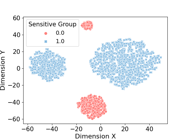
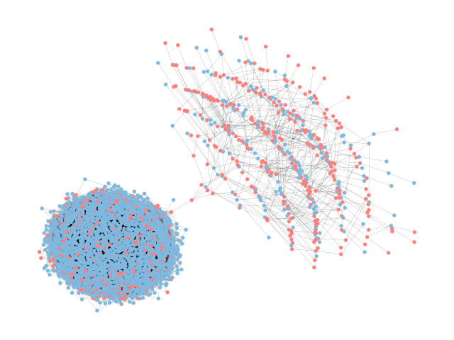
(a) Biased non-sensitive features and graph topology(Minor)

(b) Unbiased non-sensitive features and graph topology(Minor)

Figure 5. Biased and Unbiased Graph Data Synthesis

First, we identify the main sensitive attribute $S_{m}$ and the minor $S_{n}$. E.g., to investigate racism in risk assessments(SKEEM and LOWENKAMP, 2016), ’race’ is the key focus while ’age’ follows behind. The overview of the synthetic data is shown in Figure 5, wherein we visualize non-sensitive features with t-SNE(van der Maaten and Hinton, 2008). We detail the data synthesis in Appendix A.1.

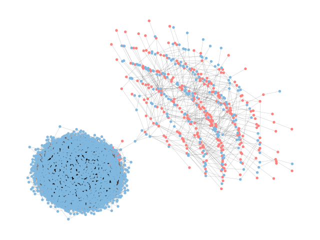
(a) Biased non-sensitive features and graph topology(Major)

(b) Unbiased non-sensitive features and graph topology(Major)

Figure 1. Biased and Unbiased Graph Data Synthesis

3.2. Case Analysis

3.2.1. Sensitive Correlation

To unify the standard pipeline, we first measure $\mathcal{R}^{2}_{n}(\mathcal{X},S)$, $\mathcal{R}^{2}_{n}(\mathcal{X}_{N},S)$ and $h_{sens}$ for $S_{n}$ and $S_{m}$, which denote sensitive distance correlations of original features and non-sensitive features, and sensitive homophily of $S_{n}$ and $S_{m}$, respectively. We next obtain the prediction $\hat{Y}$, compute $\mathcal{R}^{2}_{n}(\hat{Y},S)$, record $\Delta$SP and $\Delta$EO for $S_{n}$ and $S_{m}$, and compare them to evaluate biases. The split ratio is 1:1:8 for training, validation and test sets and we repeat the experiments 10 times to report the average results. The experimental setting is detailed in Appendix A.3.

Table 1. Sensitive Correlation in Before/After GNN Training. The results are shown in percentage($\%$). 1 represents the minor sensitive attribute while 2 denotes the major.

Cases	Before Training				After Training
	$\bm{\mathcal{R}^{2}_{n}(\mathcal{X},S)}$	$\bm{\mathcal{R}^{2}_{n}(\mathcal{X}_{N},S)}$	$\bm{h_{sens1}}$	$\bm{h_{sens2}}$	$\Delta SP_{1}$	$\Delta EO_{1}$	$\Delta SP_{2}$	$\Delta EO_{2}$	$\bm{\mathcal{R}^{2}_{n}(\hat{Y},S)}$
BFDT	72.76	72.68	56.52	65.22	22.83$\pm 6.0$	33.18$\pm 5.6$	21.95$\pm 6.3$	21.65$\pm 4.7$	17.70$\pm 0.0$
DFBT	29.50	4.46	66.89	79.70	5.17$\pm 1.7$	5.22$\pm 1.7$	12.80$\pm 2.3$	14.25$\pm 2.9$	12.70$\pm 0.0$
BFBT	72.76	72.68	66.89	79.70	4.30$\pm 3.0$	4.37$\pm 2.5$	47.94$\pm 5.7$	29.90$\pm 3.9$	22.57$\pm 0.0$
DFDT	29.50	4.46	56.53	65.22	3.35$\pm 1.6$	5.33$\pm 3.0$	12.07$\pm 2.9$	14.13$\pm 4.1$	12.57$\pm 0.0$

Case 1: Biased Features and Debiased Topology(BFDT) In Case 1, we feed biased non-sensitive features and debiased topology into GNNs. As shown in Table 1, there is only a small difference before and after masking sensitive attributes. After MP, biases from both sensitive attributes are projected into predicted results.

Case 2: Debiased Features and Biased Topology(DFBT) In Case 2, we focus on debiased features and biased topology. From Table 1, there is a relatively large difference before and after masking and the sensitive correlation is much lower and the results are fairer on both sensitive attributes and more consistent.

Case 3: Biased Feature and Topology(BFBT) In Case 3, we shift to biased non-sensitive features and topology. In Table 1, a higher sensitive correlation is introduced. We notice that the fairness performance of the major sensitive attribute is much higher than the minor, and the minor’s performance is even a bit lower than Case 2. On average, the sensitive attributes are more biased.

Case 4: Debiased Feature and Topology(DFDT) In Case 4, we turn to debiased features and topology. In Table 1, the fairness performance is close to Case 2 and the sensitive correlation reflected in the final prediction is slightly lower, which indicates that the majority of biases stem from biased node features. Graph topologies and MP mainly play complementary roles in amplifying biases.

Discussion The case analyses elucidate that node features, graph topologies and MP are all crucial bias resources, which motivates us to simultaneously debias features and topologies under MP at the pre-processing stage instead of debiasing them separately without taking MP into consideration.

3.2.2. Sensitive Information Leakage

Our work considers a universal situation where due to fair awareness or legal compliance, the data owners (e.g., research institutions or companies) release masked non-sensitive features and incomplete graph topologies to the public for specific purposes. We argue that even though the usual procedures pre-handle features and topologies that are ready for release, the sensitive information leakage problem still exists and sensitive attributes can be inferred from the aforementioned resources, which further amplify existing inequalities and cause severe social consequences. We assume that the adversaries can access pre-processed $\tilde{\mathcal{X}},\tilde{A}$ and label $\mathcal{Y}$, and then obtain partial sensitive attributes $S_{p}$ of specific individuals as prior knowledge, where $p\in\{0.3125\%,0.625\%,1.25\%,2.5\%,5\%,10\%,20\%\}$. Finally, they simply use a 1-layer GCN with a linear classifier as the attack model to identify different sensitive memberships, i.e., $S_{m}$ or $S_{n}$ of the rest nodes. We adopt the synthetic data again to explore sensitive information leakage with or without fairness intervention.

As Figure 2 shows, even though the adversaries only acquire very few $S_{m}$ or $S_{n}$, they can successfully infer the rest from all pairs since highly associated features are retained and become more sensitively correlated after MP. We note that $S_{m}$ are more biased than $S_{n}$. While there are turning points in the fewer label cases due to performance instability, with more sensitive labels to be collected, there are higher attack accuracy and sensitive correlations. In all, the BFBT pair always introduces the most biases and sensitive information leakage, the BFDT pair leads to lower sensitive correlation and attack accuracy, and the performances of DFBT and DFDT pairs are close, which indicates that compared to biased features, biased topology contributes less to inference attacks of $S_{m}$ and $S_{n}$. Once fairness interventions for features and topology are added, the overall attack accuracy stabilizes to decrease by all 10$\%$ and the sensitive correlation decreases by almost 50$\%$/40$\%$ for $S_{m}$ and $S_{n}$.

Discussion The above analysis illustrates that even simple fairness interventions can alleviate attribute inference attacks under the black-box settings. Generally, more advanced debiasing methods will result in less sensitive information leakage, which fits our intuition and motivates us to design more effective debiasing techniques with limited sensitive information leakage.

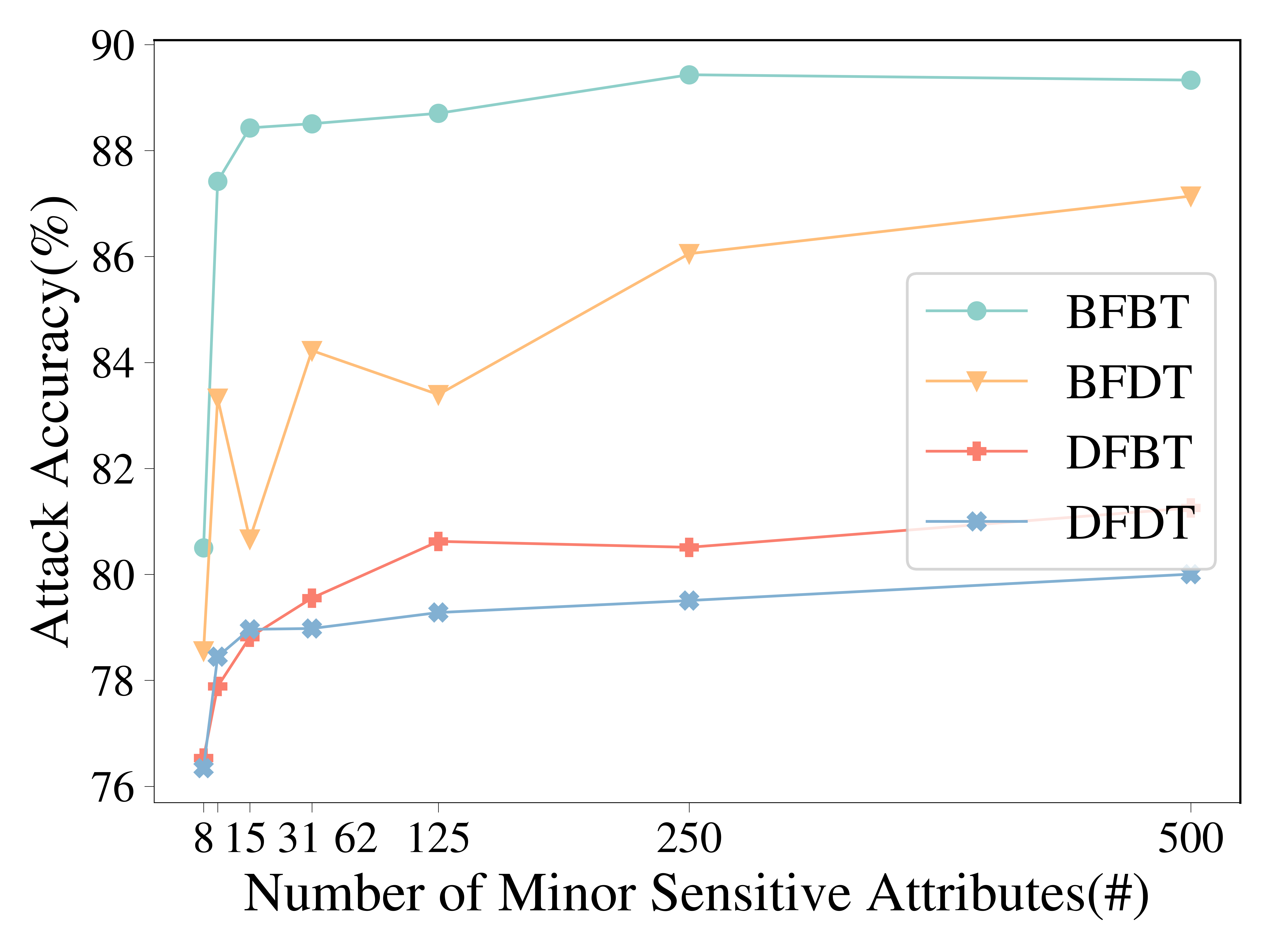
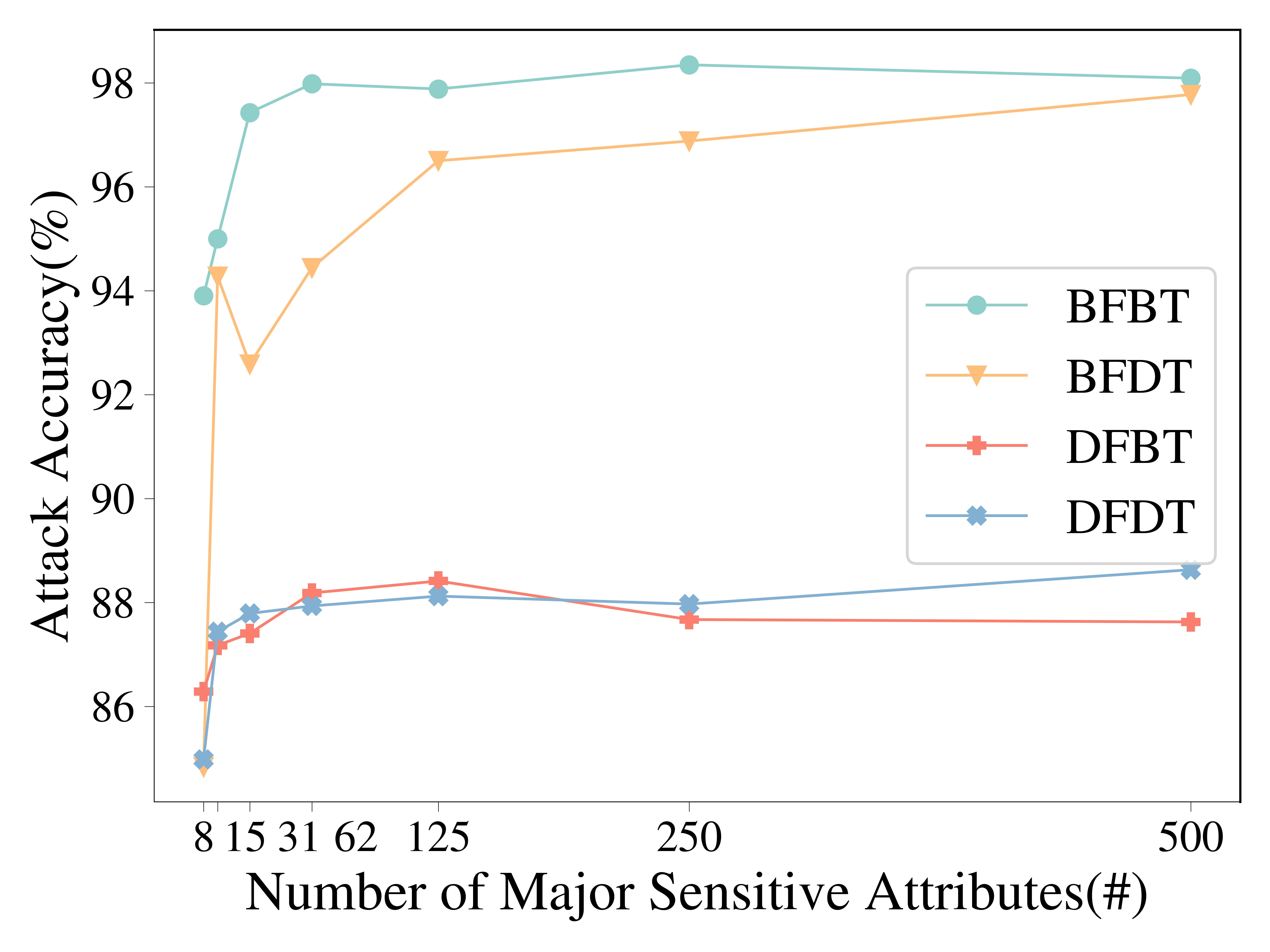
(a) Attack Accuracy

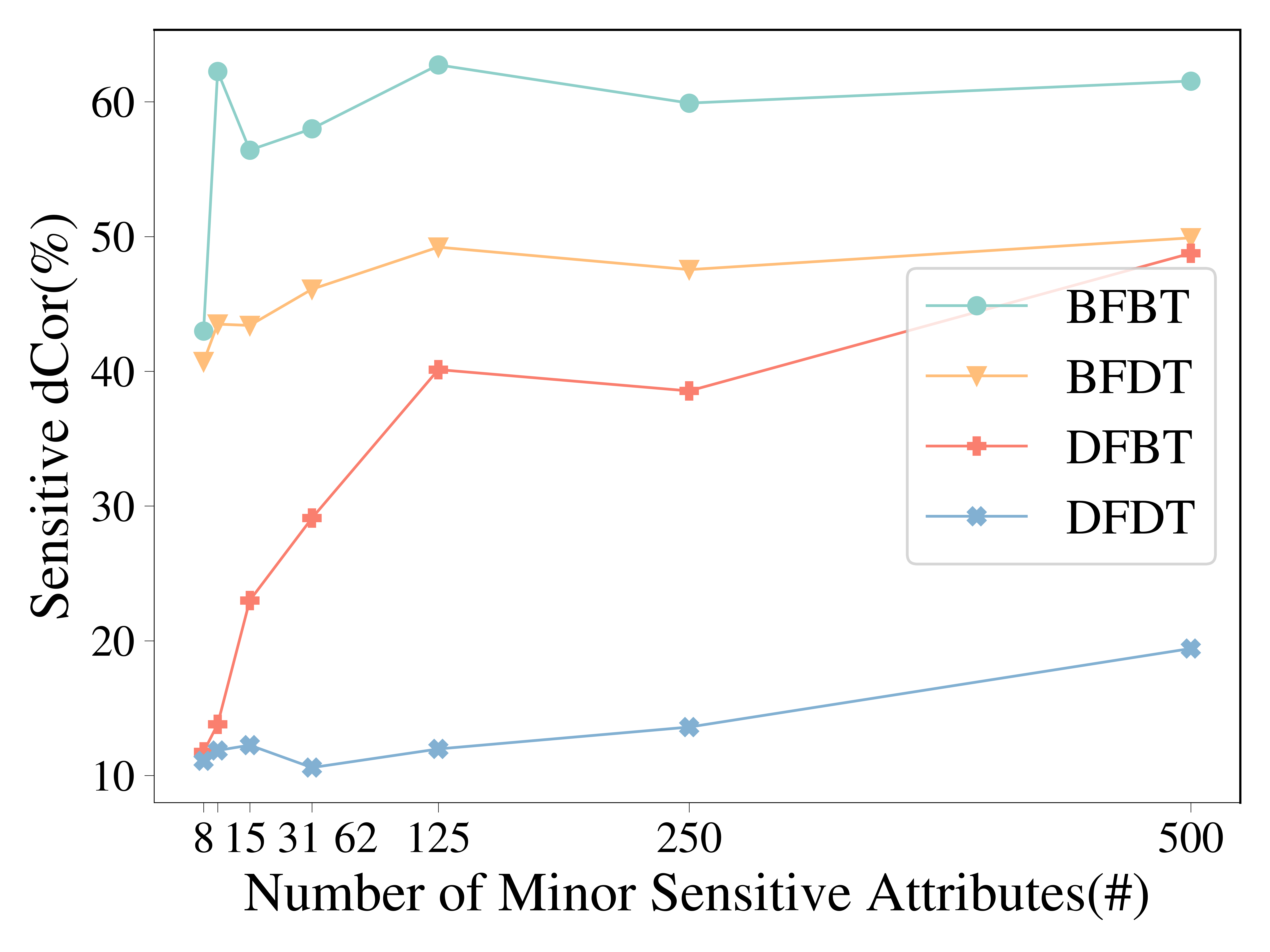
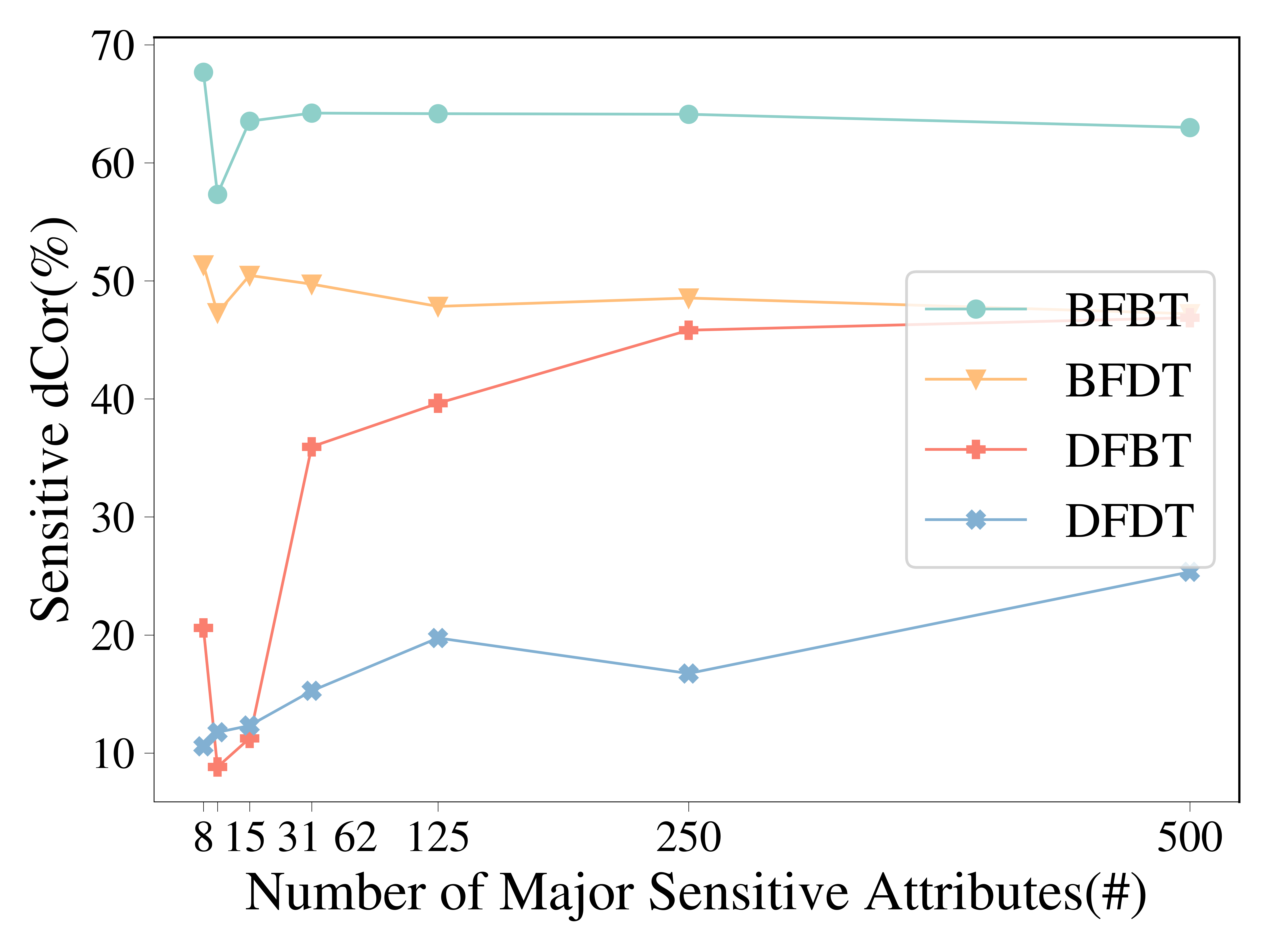
(b) Sensitive Correlation

Figure 2. Attribute Inference Attack Under Different Cases

3.3. Problem Statement

Based on the two empirical studies, we define the formal problem as: Given an undirected attributed graph $\mathcal{G}=\left(\mathcal{V},\mathcal{E},\mathcal{X}\right)$ with the sensitive attributes $S$, non-sensitive features $\mathcal{X}_{N}$, graph topology $A$ and node labels $\mathcal{Y}$, we aim to learn pre-debiasing functions $\Phi_{f}(X)=\hat{X}$ and $\Phi_{t}(A)=\hat{A}$ and thereby construct a fair and model-agnostic classifier $f_{\theta}(\hat{X},\hat{A})=\hat{Y}$ with limited sensitive information leakage.

4. Framework Design

In this section, we provide an overview of MAPPING, which consecutively debias node features and graph topologies, and then we detail each module to tackle the formulated problem.

4.1. Framework Overview

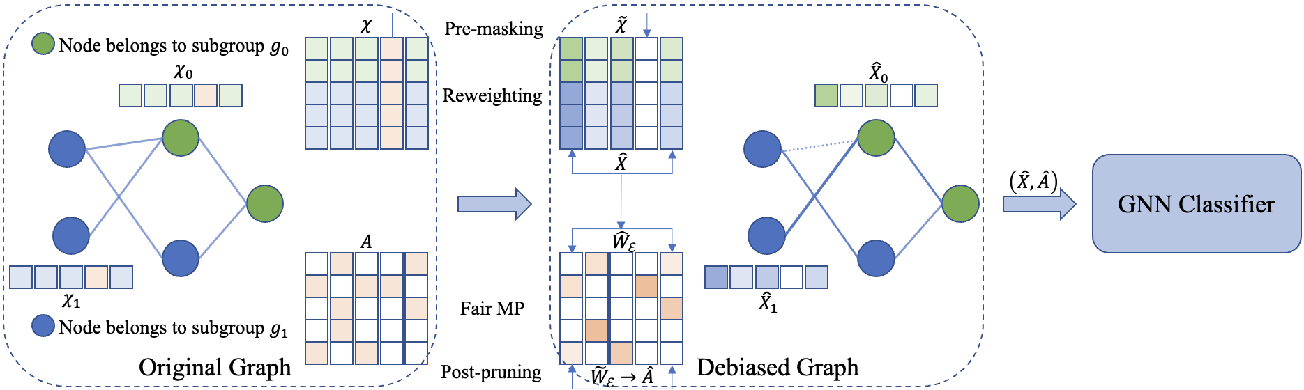
Figure 3. The Framework Overview of MAPPING with Feature and Topology Debiasing

MAPPING consists of two modules to debias node features and graph topologies. The feature debiasing module contains $1)$ pre-masking: masking sensitive attributes and their highly associated features based on hard rules to trade off utility and fairness and $2)$reweighting: reweighting the pre-masked features $\tilde{\mathcal{X}}$ to restrict attribute inference attacks by adversarial training and $dCov$-based fairness constraints. With debiased features $\hat{X}$ on hand, the topology debiasing module includes $1)$ Fair MP: initializing equalized weights $W_{0}$ for existed edges $\mathcal{E}$ and then employing a $dCov$-based fairness constraint to mitigate sensitive privacy leakage and $2)$ Post-pruning: pruning edges with weights $\hat{W}_{\mathcal{E}}$ beyond the pruning threshold $r_{p}$ to obtain $\tilde{W}_{\mathcal{E}}$ and then returning the debiased adjacency matrix $\hat{A}$. The overview of MAPPING is shown in Figure 3. And the algorithm overview is detailed in Algorithm 2 in Appendix B.

4.2. Feature Debiasing Module

4.2.1. Pre-masking

Simply removing sensitive attributes, i.e., fairness through blindness(Dwork et al., 2012), cannot sufficiently protect specific demographic groups from discrimination and attacks. $\mathcal{X}_{N}$ that are highly associated with $S$ can reveal the sensitive membership or be used to infer $S$ even without access to it(Dwork et al., 2012; Jayaraman and Evans, 2022). Furthermore, without fairness intervention, $\mathcal{Y}$ are always reflective of societal inequalities and stereotypes(Beutel et al., 2017) and $\hat{Y}$ ineluctably inherit such biases since they are predicted by minimizing the difference between $\mathcal{Y}$ and $\hat{Y}$. Inspired by these points, we first design a pre-masking method to mask $S$ and highly associated $\mathcal{X}_{N}$ with the power of $dCor$. However, we cannot simply discard all highly associated $\mathcal{X}_{N}$ since part of them may carry useful information and finally contribute to node classification. Hence, we must carefully make the trade-off between fairness and utility.

Considering above factors, we first compute $\mathcal{R}_{n}^{2}(\mathcal{X}_{i},S)$ and $\mathcal{R}_{n}^{2}(\\ \mathcal{X}_{i},\mathcal{Y})$, $i\in[1,\dots,d]$. We set a distributed ratio $r$(e.g., $20\%$) to pick up $x$ top related features based on $\mathcal{R}_{n}^{2}(\mathcal{X},S)$ and $x$ less related features based on $\mathcal{R}_{n}^{2}(\mathcal{X},\mathcal{Y})$. We then take an intersection of these two sets to acquire features that are highly associated with $S$ and simultaneously contribute less to accurate node classification. Next, we use a sensitive threshold $r_{s}$($70\%$) to filter features whose $\mathcal{R}_{n}^{2}(\mathcal{X}_{i},S)<r_{s}$. Finally, we take the union of these two sets of features to guarantee:

• We cut off very highly associated $\mathcal{X}_{N}$ to pursue fairness;

• Besides the hard rule, to promise accuracy, we scrutinize that only $\mathcal{X}$ are highly associated with $S$ and make fewer contributions to the final prediction are masked;

• The rest of the features are pre-masked features $\tilde{\mathcal{X}}$.

More details are seen in Algorithm 1 in Appendix B.

Pre-masking benefits bias mitigation and privacy preservation. Besides, it reduces the dimension of node features, thereby saving training costs, which is particularly effective on large-scale datasets with higher dimensions. However, partially masking $S$ and its highly associated $\mathcal{X}_{N}$ may not be adequate. Prior studies (Zhao et al., 2022; Zhu and Wang, 2022) have demonstrated the feasibility of $S$ estimation without accessing $S$. To tackle this issue, we further debias node features after pre-masking.

4.2.2. Reweighting

We first assign initially equal weights $W_{f_{0}}$ for $\tilde{\mathcal{X}}$. For feature $\tilde{\mathcal{X}_{i}},i\in[1,\dots,d_{m}]$, where $d_{m}$ is the dimension of masked features, if corresponding $\hat{W}_{fi}$ decreases, $\tilde{\mathcal{X}_{i}}$ plays a less important role to debias features and vice versa. Therefore, the first objective is to minimize:

(4) $$\min_{\theta_{r}}\mathcal{L}_{r}=\|\tilde{\mathcal{X}}-\hat{X}\|_{2}$$

where $\hat{X}=f_{\theta_{\hat{w}}}(\tilde{\mathcal{X}})=\tilde{\mathcal{X}}\hat{W}_{f}$.

In addition, we restrict the weight changes and control the sparsity of weights. Here we introduce $L$1 regularization as:

(5) $$\min_{\theta_{\hat{w}}}\mathcal{L}_{\hat{w}}=\|\hat{W}_{f}\|_{1}$$

Next, we introduce $dCov$-based fairness constraints. Since the same technique is utilized in fair MP, we unify them to avoid repeated discussions. The ideal cases are $\hat{X}\perp S$ and $\hat{Y}\perp S$, which indicates that the sensitive attribute inference derived from $\hat{X}$ and $\hat{Y}$ are close to random guessing. Zafar et al.(Zafar et al., 2017) and Dai et al.(Dai and Wang, 2021) employ $Cov$-based constraints to learn fair classifiers. However, $Cov$ needs pairwise computation, and it ranges from $-\infty$ to $\infty$, which require adding the extra absolute form. Moreover, $Cov=0$ cannot ensure independence but only reflect irrelevance. Cho et al.(Cho et al., 2020) and Roh et al.(Roh et al., 2020) use $MI$-based constraints for fair classification. Though $MI$ uncovers mutual independence between random variables, it cannot get rid of dimensional restrictions. Whereas $dCov$ can overcome these deficiencies. $dCov$ reveals independence and it is larger than $0$ for dependent cases. Above all, it breaks dimensional limits and thereby saves computation costs. Hence, we leverage a $dCov$-based fairness constraint in our optimization, marked as:

(6) $$\mathcal{L}_{s}=\mathcal{V}_{n}^{2}(\hat{X},S)$$

Finally, we use adversarial training(Zhang et al., 2018) to mitigate sensitive privacy leakage by maximizing the classification loss as:

(7) $$\max_{\theta_{a}}\mathcal{L}_{a}=-\frac{1}{n}\sum_{i=1}^{n}S_{i}\log(\hat{S}_{i})+(1-S_{i})\log(1-\hat{S}_{i})$$

where $\hat{S}=f_{\theta_{{s}}}(\hat{X})$.

Cho et al.(Cho et al., 2020) empirically shows that adversarial training suffers from significant stability issues and $Cov$-based constraints are commonly adopted to alleviate such instability. In this paper, we use $dCov$ to achieve the same goal.

4.2.3. Final Objective Function of Feature Debiasing

Now we have $f_{\theta_{r}}$ to minimize feature reconstruction loss, $f_{\theta_{\hat{w}}}$ to restrict weights, $f_{\theta_{a}}$ to debias adversarially, and $\mathcal{L}_{s}$ to diminish sensitive information disclosure. In summary, the final objective function of the feature debiasing module is:

(8) $$\min_{\theta_{r},\theta_{\hat{w}},\theta_{a}}\mathcal{L}_{r}+\lambda_{1}\mathcal{L}_{\hat{w}}+\lambda_{2}\mathcal{L}_{s}-\lambda_{3}\mathcal{L}_{a}$$

where $\theta_{r}$, $\theta_{\hat{w}}$ and $\theta_{a}$ denote corresponding objective functions’ parameters. Coefficients $\lambda_{1}$, $\lambda_{2}$ and $\lambda_{3}$ control weight sparsity, sensitive correlation and adversarial debiasing, respectively.

4.3. Topology Debiasing Module

4.3.1. Fair MP

Prior work(Dai and Wang, 2021) empirically demonstrates biases can be magnified by graph topologies and MP. FMP(Jiang et al., 2022) investigates how topologies can enhance biases during MP. Our empirical analysis likewise reveals that sensitive correlations increase after MP. Here we propose a novel debiasing method to jointly debias topologies under MP, which is conducive to providing post-pruning with explanations of edge importance.

First, we initialize equal weights $W_{{\mathcal{E}_{0}}}$ for $\mathcal{E}$, then feed $W_{{\mathcal{E}}_{0}}$, $A$ and $\hat{X}$ into GNN training. The main goal of node classification is to pursue accuracy, which equalizes to minimize:

(9) $$\min_{\theta_{\mathcal{C}}}\mathcal{L}_{\mathcal{C}}=-\frac{1}{n}\sum_{i=1}^{n}\mathcal{Y}_{i}\log(\hat{Y}_{i})+(1-\mathcal{Y}_{i})\log(1-\hat{Y}_{i})$$

As mentioned before, we add a $dCov$-based fairness constraint into the objective function to ameliorate sensitive attribute inference attacks derived from $\hat{Y}$. Defined as:

(10) $$\mathcal{L}_{\mathcal{F}}=\mathcal{V}^{2}_{n}(\hat{Y},S)$$

4.3.2. Final Objective Function of Topology Debiasing

Now we have $f_{\theta_{\mathcal{C}}}$ to minimize node classification loss and $\mathcal{L}_{\mathcal{F}}$ to restrain sensitive information leakage. The final objective function of topology debiasing module can be written as:

(11) $$\min_{f_{\theta_{\mathcal{C}}}}\mathcal{L}_{e}=\mathcal{L}_{\mathcal{C}}+\lambda_{4}\mathcal{L}_{\mathcal{F}}$$

Where $\theta_{\mathcal{C}}$ denotes the parameter of the node classifier $\mathcal{C}$, the coefficient $\lambda_{4}$ controls the balance between utility and fairness.

4.3.3. Post-pruning

After learnable weights $\hat{W}_{\mathcal{E}}$ have been updated to construct a fair node classifier with limited sensitive information leakage, we apply a hard rule to prune edges with edge weights $\hat{W}_{e_{i}\cdot}$ for $e_{i\cdot}\in\mathcal{E}$ that are beyond the pruning threshold $r_{p}$. Please note, since we target undirected graphs, if any two nodes $i$ and $j$ are connected, $\hat{W}_{e_{ij}}$ should be equal to $\hat{W}_{e_{ji}}$, which assures $A_{ij}=A_{ji}$ after pruning. Mathematically,

(12) $$\tilde{W}_{ei}=\begin{cases}1,&\mbox{if }\hat{W}_{e_{i\cdot}}\geq r_{p}\\ 0,&\mbox{otherwise}\end{cases}$$

$$s.t.,\hat{W}_{e_{ij}}=\hat{W}_{e_{ji}},\mbox{ if }e_{ij}\in\mathcal{E}$$

Removing edges is practical since edges can be noisy in reality, and meanwhile, they can exacerbate biases and leak privacy under MP. $\hat{W}_{e_{i}}$ explains which edges contribute less/more to fair node classification. We simply discard identified uninformative and biased edges. The rest forms the new $\hat{A}$.

4.4. Extension to Multiple Sensitive Attributes

Since $dCor$ and $dCov$ are not limited by dimensions, our work can be easily extended into the pre-masking strategy and adding $dCov$-based fairness constraints $\mathcal{L}_{s}$ and $\mathcal{L}_{\mathcal{F}}$ with multiple sensitive attributes as we directly calculate in previous sections. As for adversarial training, the binary classification loss cannot be trivially extended to multiple sensitive labels. Previously in the reweighting strategy, we simply adopted $f_{\theta_{s}}$ to map estimated masked features with $d_{m}$ into a single predicted sensitive attribute. Instead, in the multiple case, we map the features into predicted multiple sensitive attributes with the desired dimensions $d_{s}$. Next, we leverage the function (7) to compute the classification loss for each sensitive attribute and then we can take the average or other forms of all losses. The rest steps are exactly the same as described before.

5. Experiments

In this section, we implement a series of experiments to demonstrate the effectiveness and flexibility of MAPPING with different GNN variants. Particularly, we address the following questions:

• Q1: Does MAPPING effectively and efficiently debias feature and topology biases hidden behind graphs?

• Q2: Does MAPPING flexibly adapt to different GNNs?

• Q3: Does MAPPING outperform existing pre-processing and in-processing algorithms for fair node classification?

• Q4: Whether MAPPING can achieve better trade-offs between utility and fairness and meanwhile mitigate sensitive information leakage?

• Q5: How debiasing contribute to fair node classification?

5.1. Experimental Setup

In this subsection, we first describe the datasets, metrics and baselines, and then summarize the implementation details.

5.1.1. Datasets

We validate MAPPING on $3$ real-world datasets, namely, German, Recidivism and Credit(Agarwal et al., 2021). The detailed statistics are summarized in Table 2 and more contents are in Appendix C.1.

Table 2. Statistics Summary of Datasets

Dataset	German	Recidivism	Credit
# Nodes	1000	18,876	30,000
# Edges	22,242	321,308	1,436,858
# Features	27	18	13
Sensitive Attr.	Gender(Male/female)	Race(Black/white)	Age($\leq 25$/$>25$)
Label	Good/bad credit	Bail/no bail	Default/no default

5.1.2. Evaluation Metrics

We adopt accuracy(ACC), F1 and AUROC to evaluate utility and $\Delta_{SP}$ and $\Delta_{EO}$ to measure fairness.

5.1.3. Baselines

We investigate the effectiveness and flexibility of MAPPING on three representative GNNs, namely, GCN, GraphSAGE (Hamilton et al., 2017) and GIN(Xu et al., 2019), and compare MAPPING with three state-of-the-art debiasing models.

Vanilla GCN leverages a convolutional aggregator to sum propagated features from local neighborhoods. GraphSAGE aggregates node features from local sampled neighbors, which is more scalable to handle unseen nodes. GIN emphasizes the expressive power of graph-level representation to satisfy the Weisfeiler-Lehman graph isomorphism test(Weisfeiler and Lehman, 1968).

State-of-the-art(SODA) Debiasing Models We choose one pre-proces -sing model, namely EDITS(Dong et al., 2022) and two in-processing models, namely, FairGNN(Dai and Wang, 2021) and NIFTY(Agarwal et al., 2021). Since NIFTY(Agarwal et al., 2021) targets fair node representation, we evaluate the quality of node representation on the downstream node classification task.

5.1.4. Implementation Details

We keep the same experiment setting as before. The GNNs follow the same architectures in NIFTY (Agarwal et al., 2021). The fine-tuning processes are handled with Optuna(Akiba et al., 2019) via the grid search. As for feature debiasing, we deploy a $1$-layer multilayer perceptron(MLP) for adversarial debiasing and leverage the proximal gradient descent method to optimize $W_{f}$. Since PyTorch Geometric only allows positive weights, we use a simple sigmoid function to transfer weights into $[0,1]$. We set the learning rate as $0.001$ and the weight decay as 1e-5 for all the three datasets, and set training epochs as $500$. For topology debiasing, we adopt a $1$-layer GCN to mitigate biases under MP. We set training epochs as $1000$ for all datasets, as for GIN in Credit, since small epochs can achieve comparable performance, we set early stopping to avoid overfitting. Others are the same as feature debiasing. As for GNN training, we utilize the split setting in NIFTY(Agarwal et al., 2021), we fix the hidden layer as $16$, the dropout as $0.2$, training epochs as $1000$, weight decay as 1e-5 and learning rate from $\{0.01,0.03\}$ for all GNNs. For fair comparison, we rigorously follow the settings in SODA(Dai and Wang, 2021; Agarwal et al., 2021; Dong et al., 2022). The other detailed hyperparameter settings are in Appendix C.2.

The attack setting is the same as before to evaluate sensitive information leakage. Still, we repeat experiments $10$ times with $10$ different seeds and finally report the average results.

5.2. Performance Evaluation

In this subsection, we evaluate the performance by addressing the top $4$ questions raised at the beginning of this section.

5.2.1. Debiasing Effectiveness and Efficiency

To answer Q1, we first compute $\Delta$SP and $\Delta$EO before and after debiasing and then evaluate the debiasing effectiveness. Second, we provide the time complexity analysis to illustrate the efficiency of MAPPING.

Effectiveness The results shown in Table 3 demonstrate the impressive debiasing power of MAPPING in node classification tasks. Compared to vanilla GNNs, $\Delta SP$ and $\Delta EO$ in Table 3 all decrease, especially in German, GNNs drop more biases than in Recidivism and Credit, wherein GCN introduces more biases than other GNN variants but reduces more biases as well in most cases.

Efficiency Once pre-debiasing is completed, the rest training time purely reflects the efficiency of vanilla GNNs. Generally, the summed running time of pre-debiasing and GNN training is lower than in-processing methods which introduce extra computational costs, e.g., complex objective functions and/or iterative operations. Even in the small-scale German dataset, the whole running time of MAPPING is always less than $150$ seconds for $10$ trials, but FairGNN(Dai and Wang, 2021) and NIFTY(Agarwal et al., 2021)(excluding counterfactual fairness computation) are $1.17$-$9.28$ times slower. Since we directly use EDITS’s (Dong et al., 2022) debiased datasets, there is no comparison for pre-debiasing, but EDITS is $1.00$-$6.43$ times slower in running GNNs. We argue that MAPPING modifies more features and edges but still achieves competitive debiasing and classification performance. Concerning time complexity, the key lies in $dCov$ and $dCor$ calculations, which is $\mathcal{O}(|\mathcal{V}|^{2})$(Huang and Huo, 2022). For feature debiasing, the time complexity of pre-masking is $\mathcal{O}(d|\mathcal{V}|^{2})$, where $d$ is the dimension of original features. Since $d$ is small, the time complexity is comparable to $\mathcal{O}(|\mathcal{V}|^{2})$; the time complexity of reweighting for each training epoch is $2\mathcal{O}(|\mathcal{V}|^{2})+\mathcal{O}(d)$, which is comparable to $\mathcal{O}(|\mathcal{V}|^{2})$. As for topology debiasing, fair MP is in time complexity of $\mathcal{O}(|\mathcal{V}|^{2})+\mathcal{O}(|\mathcal{V}|)$ for each training epoch and post-pruning is $\mathcal{O}(|\mathcal{E}|)$. As suggested in (Huo and Székely, 2016), the time complexity of $dCov$ can be further reduced to $\mathcal{O}(|\mathcal{V}|\log(|\mathcal{V}|))$ for univariate cases.

5.2.2. Framework Flexibility and Model Performance

To answer Q2 to Q4, we compare MAPPING against other baselines and launch attribute inference attacks to investigate the effects of sensitive information leakage mitigation of MAPPING.

Flexibility To answer Q2, from Table 3, we observe that compared to vanilla GNNs, MAPPING improves utility in most cases, especially training German with GIN, and Recidivism with GCN and GraphSAGE. We argue that MAPPING can remove features that contribute less to node classification and meanwhile delete redundant and noisy edges. Plus the debiasing analysis, we conclude that MAPPING can flexibly adapt to diverse types of GNN variants.

Model Comparison and Trade-offs To answer Q3, we observe that MAPPING achieves more competitive performance than other SODA models. In view of utility, MAPPING more or less outperforms in one or more utility metrics in all cases. It even outperforms all other baselines in all metrics when training German with GIN and Recidivism with GCN. With respect to fairness, on most occasions, all debiasing models can effectively alleviate biases, wherein MAPPPING outperforms others. Moreover, MAPPING is more stable than the rest. Overall, we conclude that MAPPING achieves better utility and fairness trade-offs than the baselines.

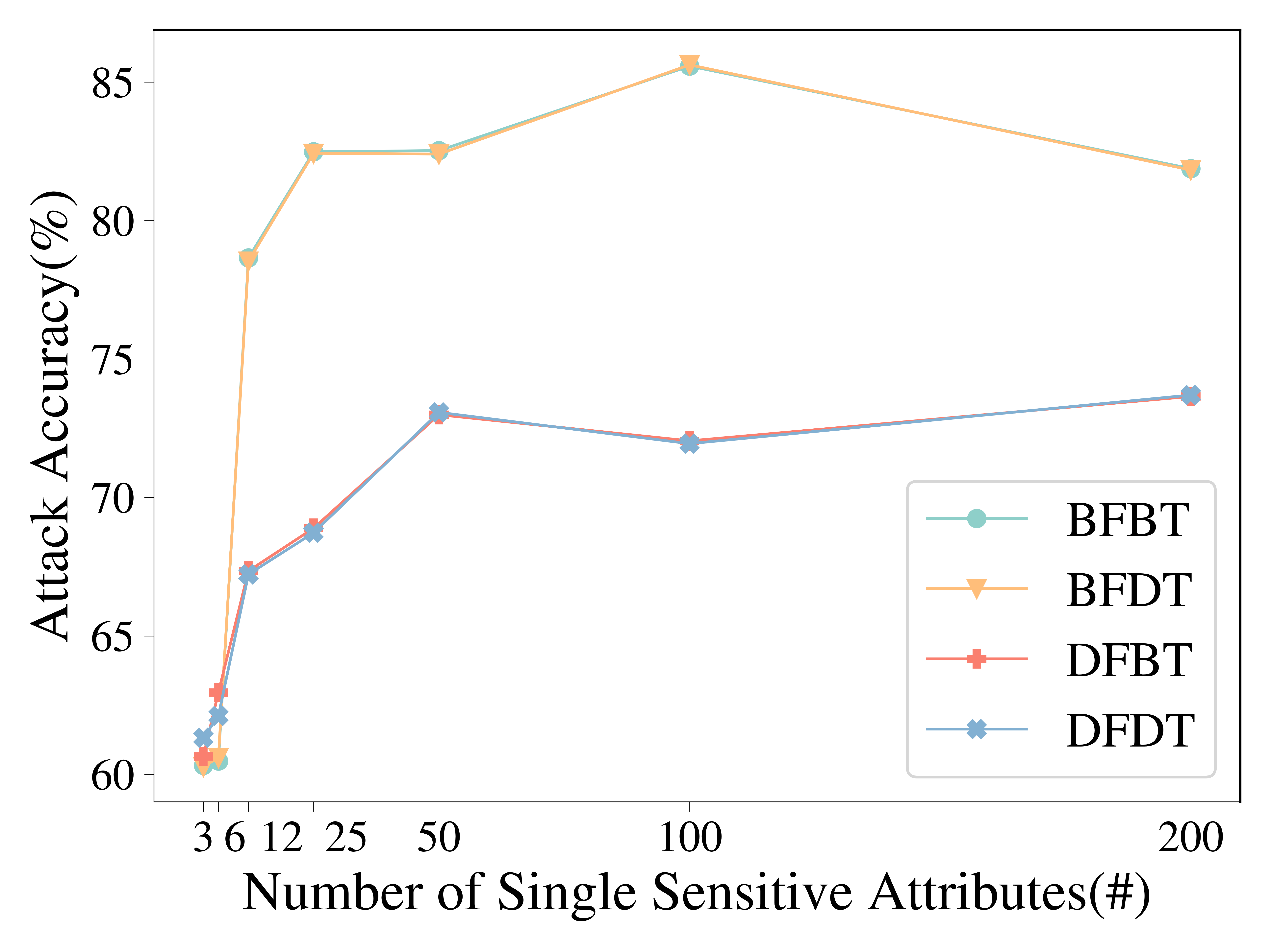
(a)

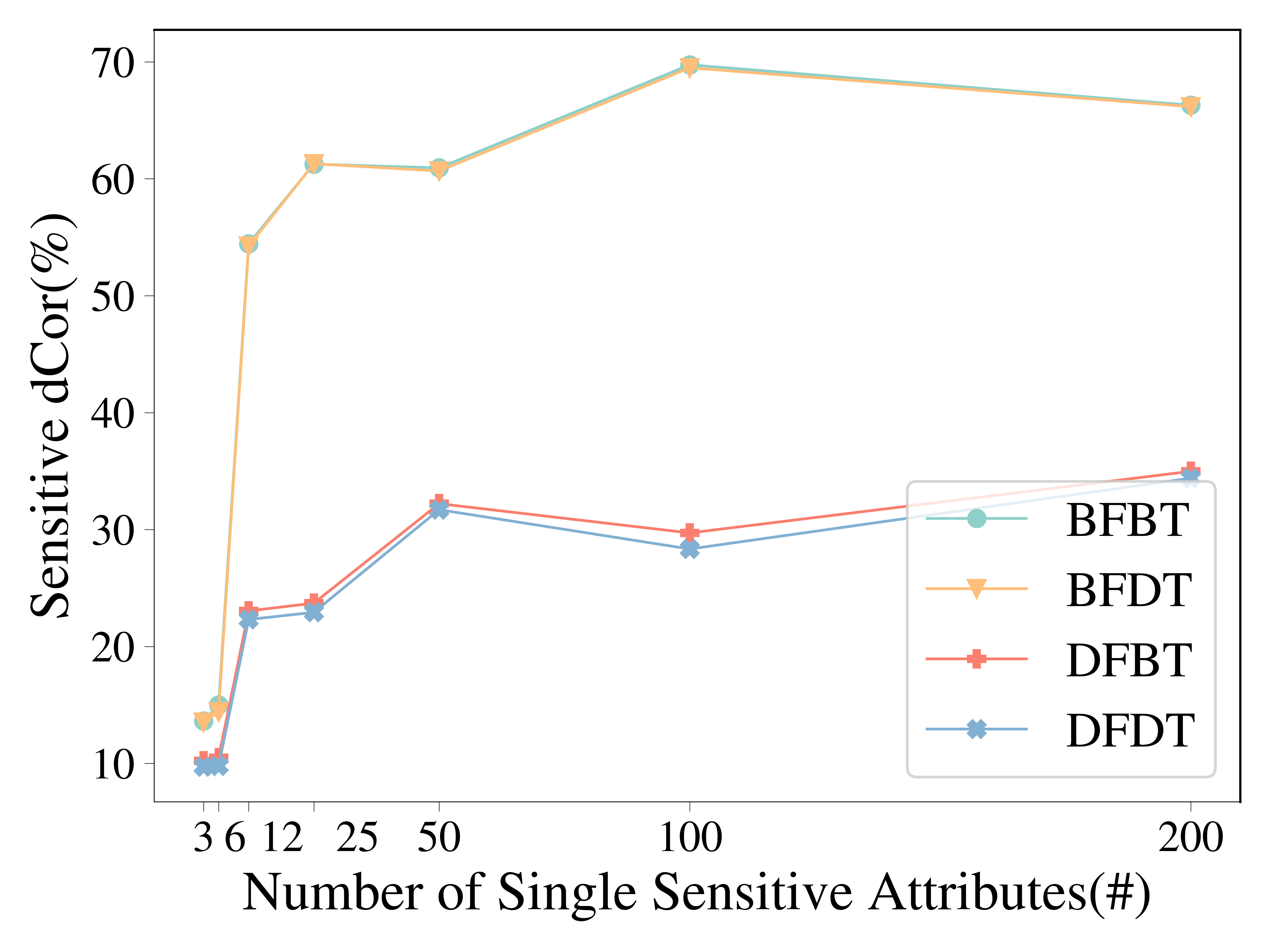
(b)

Figure 4. Attribute Inference Attack Under Different Inputs

Sensitive Information Leakage To answer Q4, since German reduces the largest biases, we simply use German to explore sensitive information leakage under different input pairs. As shown in Figure 4, since all sensitive attributes are masked and MAPPING only prunes a small portion of edges in German, the attack accuracy and sensitive correlation of BFBT pair are quite close to the BFDT pair while DFDT’s performance is slightly lower than the DFBT pair, which further verifies the aforementioned empirical findings and elucidates that MAPPING can effectively confine attribute inference attacks even when adversaries can collect large numbers of sensitive labels. Please note that there are some performance drops, we argue it is due to the combined effects of data imbalance and more stable performance after collecting more sensitive labels.

5.3. Extension to Multiple Sensitive Attributes

We set the main sensitive attribute as gender and the minor as age$\left(\leq 25/>25\right)$. Still, we adopt German to perform evaluation and explore sensitive information leakage. The details follow the same pattern in Subsection 5.2 and more are shown in Appendix C.3.

Table 3. Node classification performance comparison on German, Recidivism and Credit.

GNN	Framework	German					Recidivism					Credit
		ACC	F1	AUC	$\Delta$SP	$\Delta$EO	ACC	F1	AUC	$\Delta$SP	$\Delta$EO	ACC	F1	AUC	$\Delta$SP	$\Delta$EO
GCN	Vanilla	72.00$\pm 2.8$	80.27$\pm 2.5$	74.34$\pm 2.4$	31.42$\pm 9.5$	22.56$\pm 6.2$	87.54$\pm 0.1$	82.51$\pm 0.1$	91.11$\pm 0.1$	9.28$\pm 0.1$	8.19$\pm 0.3$	76.19$\pm 0.4$	84.22$\pm 0.4$	73.34$\pm 0.0$	9.00$\pm 1.2$	6.12$\pm 0.9$
	FairGNN	67.80$\pm 11.0$	74.10$\pm 17.6$	73.08$\pm 2.0$	24.37$\pm 8.7$	16.99$\pm 6.8$	87.50$\pm 0.2$	83.40$\pm 0.2$	91.53$\pm 0.1$	9.17$\pm 0.2$	7.93$\pm 0.4$	73.78$\pm 0.1$	82.01$\pm 0.0$	73.28$\pm 0.0$	12.29$\pm 0.6$	10.04$\pm 0.7$
	NIFTY	66.68$\pm 8.6$	73.59$\pm 13.4$	70.59$\pm 4.8$	15.65$\pm 9.2$	10.58$\pm 7.3$	76.67$\pm 1.8$	69.09$\pm 0.9$	81.27$\pm 0.4$	3.11$\pm 0.4$	2.78$\pm 0.5$	73.33$\pm 0.1$	81.62$\pm 0.1$	72.08$\pm 0.1$	11.63$\pm 0.2$	9.32$\pm 0.2$
	EDITS	69.80$\pm 3.2$	80.18$\pm 2.2$	67.57$\pm 6.0$	4.85$\pm 2.8$	4.93$\pm 2.2$	84.82$\pm 0.8$	78.56$\pm 1.1$	87.42$\pm 0.7$	7.23$\pm 0.3$	4.43$\pm 0.7$	75.20$\pm 1.7$	84.11$\pm 2.2$	68.63$\pm 5.8$	5.33$\pm 3.8$	3.64$\pm 2.7$
	MAPPING	70.84$\pm 1.8$	81.33$\pm 1.3$	70.86$\pm 1.9$	4.54$\pm 2.2$	4.00$\pm 1.7$	88.91$\pm 0.2$	84.17$\pm 0.4$	93.31$\pm 0.1$	2.81$\pm 0.2$	0.73$\pm 0.3$	76.73$\pm 0.2$	84.81$\pm 0.2$	73.26$\pm 0.0$	1.39$\pm 0.4$	0.21$\pm 0.2$
GraphSAGE	Vanilla	71.76$\pm 1.4$	81.86$\pm 0.8$	71.10$\pm 3.1$	14.00$\pm 8.4$	7.10$\pm 4.9$	85.91$\pm 3.2$	81.20$\pm 2.9$	90.42$\pm 1.3$	4.42$\pm 3.1$	3.34$\pm 2.2$	78.68$\pm 0.8$	86.57$\pm 0.7$	74.22$\pm 0.4$	19.49$\pm 5.8$	15.92$\pm 5.5$
	FairGNN	73.80$\pm 1.4$	81.13$\pm 1.1$	74.37$\pm 1.0$	20.94$\pm 4.0$	12.05$\pm 3.8$	87.83$\pm 1.0$	83.06$\pm 1.1$	91.72$\pm 0.5$	3.73$\pm 1.9$	4.97$\pm 2.7$	72.99$\pm 1.9$	81.28$\pm 1.7$	75.60$\pm 0.2$	11.63$\pm 4.9$	9.592$\pm 5.0$
	NIFTY	70.04$\pm 2.2$	78.77$\pm 2.5$	73.02$\pm 2.2$	16.93$\pm 8.0$	11.08$\pm 6.5$	84.53$\pm 6.5$	80.30$\pm 4.7$	91.99$\pm 0.8$	5.92$\pm 1.2$	4.54$\pm 1.5$	73.64$\pm 1.5$	81.89$\pm 1.3$	73.33$\pm 0.2$	11.51$\pm 1.0$	9.05$\pm 0.9$
	EDITS	69.76$\pm 1.5$	80.23$\pm 1.8$	69.35$\pm 1.5$	4.52$\pm 3.3$	6.03$\pm 5.5$	85.13$\pm 1.1$	78.64$\pm 1.3$	89.36$\pm 0.9$	6.75$\pm 1.0$	5.14$\pm 1.2$	74.06$\pm 2.0$	82.34$\pm 1.8$	74.12$\pm 1.3$	13.00$\pm 8.6$	11.42$\pm 9.1$
	MAPPING	70.76$\pm 1.2$	81.51$\pm 0.7$	69.89$\pm 1.9$	3.73$\pm 3.1$	2.39$\pm 1.5$	87.30$\pm 0.8$	82.07$\pm 1.2$	91.41$\pm 0.9$	3.54$\pm 1.9$	3.27$\pm 1.8$	80.19$\pm 0.3$	88.24$\pm 0.2$	74.07$\pm 0.6$	4.93$\pm 0.8$	2.57$\pm 0.6$
GIN	Vanilla	71.88$\pm 1.5$	81.93$\pm 0.7$	67.21$\pm 10.3$	14.07$\pm 10.6$	9.78$\pm 8.2$	87.62$\pm 3.7$	83.44$\pm 4.5$	91.05$\pm 3.1$	9.92$\pm 2.6$	7.75$\pm 2.1$	74.82$\pm 1.9$	83.31$\pm 2.1$	73.84$\pm 1.2$	9.40$\pm 4.5$	7.37$\pm 3.8$
	FairGNN	65.32$\pm 10.4$	72.31$\pm 17.8$	66.07$\pm 8.7$	13.67$\pm 11.8$	10.91$\pm 11.2$	84.32$\pm 1.8$	80.30$\pm 2.1$	90.19$\pm 1.3$	8.15$\pm 2.4$	6.28$\pm 1.4$	72.22$\pm 0.5$	80.67$\pm 0.4$	74.87$\pm 0.2$	12.52$\pm 3.2$	10.56$\pm 3.6$
	NIFTY	64.96$\pm 5.9$	72.62$\pm 7.8$	67.70$\pm 4.1$	11.36$\pm 6.3$	10.07$\pm 6.9$	83.52$\pm 1.6$	77.18$\pm 3.1$	87.56$\pm 0.9$	6.09$\pm 0.9$	5.65$\pm 1.1$	75.88$\pm 0.7$	83.96$\pm 0.8$	72.01$\pm 0.5$	11.36$\pm 1.8$	8.95$\pm 1.5$
	EDITS	71.12$\pm 1.5$	81.63$\pm 1.3$	69.91$\pm 1.8$	3.04$\pm 2.6$	3.47$\pm 3.3$	75.73$\pm 7.8$	65.56$\pm 10.3$	77.57$\pm 9.1$	4.22$\pm 1.4$	3.35$\pm 1.2$	76.68$\pm 0.8$	85.15$\pm 0.7$	70.91$\pm 2.0$	5.52$\pm 3.9$	4.76$\pm 2.8$
	MAPPING	73.40$\pm 1.2$	83.18$\pm 0.5$	71.48$\pm 0.6$	2.20$\pm 1.4$	2.44$\pm 1.7$	82.69$\pm 3.0$	78.43$\pm 2.6$	90.12$\pm 1.4$	2.54$\pm 1.4$	1.63$\pm 1.2$	78.28$\pm 1.0$	86.67$\pm 1.0$	72.00$\pm 1.6$	5.08$\pm 3.6$	3.92$\pm 2.9$

5.4. Impact Studies

To answer Q5, we conduct ablation and parameter studies to explore how each debiasing process in MAPPING contributes to fair node classification. As before, we solely adopt German to illustrate the impact of each process.

5.4.1. Ablation Studies

MAPPING is composed of two modules and corresponding four processes, namely, pre-masking, and reweighting for the feature debiasing module, and fair MP and post-pruning for the topology debiasing module. We test different MAPPING variants from down-top perspectives, i.e, we first train without pre-masking(w/o-msk), then train without reweighting(w/o-re), and finally train without the feature debiasing module(w/o-fe). However, the pipeline is different for topology debiasing. Since post-pruning is tightly associated with fair MP, updated edge weights may not be all equal to $0$, which requires considering all possible edges. To avoid undesired computational costs, we treat training without post-pruning and training without topology debiasing module(w/o-to) as the same case. In turn, if we directly remove fair MP, there is no edge to modify. Thus we purely consider training without the topology debiasing module.

As shown in Table 4, w/o-msk or w/o-re leads to more biases and w/o-fe results in the most biases, while w/o-to introduces less bias than other variants. In most cases, different variants sacrifice fairness for utility. The results verify the necessity of each module and corresponding processes to alleviate biases, and demonstrate comparable performance in utility.

Table 4. Ablation Studies on German

GNN	Variants	ACC	F1	AUC	$\Delta$SP	$\Delta$EO
GCN	Vanilla	72.00$\pm 2.8$	80.27$\pm 2.5$	74.34$\pm 2.4$	31.42$\pm 9.5$	22.56$\pm 6.2$
	w/o-msk	71.56$\pm 0.7$	80.93$\pm 1.0$	72.60$\pm 1.6$	17.37$\pm 7.7$	13.26$\pm 6.6$
	w/o-re	68.56$\pm 12.4$	73.37$\pm 22.7$	72.74$\pm 3.5$	16.82$\pm 6.5$	10.67$\pm 4.8$
	w/o-fe	72.40$\pm 2.0$	81.37$\pm 1.3$	72.86$\pm 4.3$	25.70$\pm 17.0$	18.07$\pm 11.8$
	w/o-to	70.44$\pm 1.6$	80.03$\pm 1.8$	72.05$\pm 1.0$	5.90$\pm 2.3$	4.20$\pm 2.3$
	MAPPING	70.84$\pm 1.8$	81.33$\pm 1.3$	70.86$\pm 1.9$	4.54$\pm 2.2$	4.00$\pm 1.7$
GraphSAGE	Vanilla	71.76$\pm 1.4$	81.86$\pm 0.8$	71.10$\pm 3.1$	14.00$\pm 8.4$	7.10$\pm 4.9$
	w/o-msk	70.52$\pm 1.9$	81.19$\pm 0.9$	69.46$\pm 3.9$	8.79$\pm 7.7$	5.16$\pm 5.0$
	w/o-re	72.36$\pm 2.0$	82.34$\pm 1.1$	71.08$\pm 2.2$	8.88$\pm 6.2$	4.20$\pm 2.6$
	w/o-fe	72.84$\pm 1.1$	82.39$\pm 0.7$	71.87$\pm 3.0$	16.75$\pm 7.8$	9.59$\pm 5.4$
	w/o-to	70.76$\pm 1.2$	81.50$\pm 0.6$	68.75$\pm 4.1$	4.94$\pm 4.8$	2.80$\pm 2.7$
	MAPPING	70.76$\pm 1.2$	81.51$\pm 0.7$	69.89$\pm 1.9$	3.73$\pm 3.1$	2.39$\pm 1.5$
GIN	Vanilla	71.88$\pm 1.5$	81.93$\pm 0.7$	67.21$\pm 10.3$	14.07$\pm 10.6$	9.78$\pm 8.2$
	w/o-msk	73.24$\pm 1.1$	83.25$\pm 0.5$	71.49$\pm 2.0$	7.22$\pm 4.7$	2.68$\pm 4.1$
	w/o-re	73.96$\pm 2.1$	83.46$\pm 0.8$	70.79$\pm 4.4$	3.46$\pm 2.5$	1.68$\pm 1.6$
	w/o-fe	74.08$\pm 0.8$	83.53$\pm 0.2$	73.02$\pm 0.6$	18.10$\pm 8.1$	9.82$\pm 7.2$
	w/o-to	72.92$\pm 1.9$	82.88$\pm 1.0$	70.49$\pm 1.1$	2.19$\pm 1.5$	3.21$\pm 2.2$
	MAPPING	73.40$\pm 1.2$	83.18$\pm 0.5$	71.48$\pm 0.6$	2.20$\pm 1.4$	2.44$\pm 1.7$

5.4.2. Parameter Studies

We mainly focus on the impacts of fairness-relevant coefficients $\lambda_{2}$, $\lambda_{3}$ for feature debiasing and $\lambda_{4}$ and $r_{p}$ for topology debiasing. The original choices are 3.50e4, 0.02, 1.29e4, 0.65 for German, 5e4, 100, 515 and 0.72 for Recidivism, and 8e4, 100, 1.34e5 and 0.724 for Credit, respectively. Still, we employ German to illustrate. Please note that we fix the pruning threshold $r_{p}$ and only investigate coefficients in objective functions. We vary $\lambda_{2}\in$ {0, 1e-5, 1e-3, 1, 1e3, 1e5, 1e7} when $\lambda_{3}$ and $\lambda_{4}$ are fixed, and alter $\lambda_{3}\in$ {0, 1e-7, 1e-5, 1e-3, 1, 1e3, 1e5} when $\lambda_{2}$ and $\lambda_{4}$ are fixed, and finally change $\lambda_{4}\in${0, 1e-5, 1e-3, 1, 1e3, 1e5, 1e7} when $\lambda_{2}$ and $\lambda_{3}$ are fixed. As shown in Appendix C.4, the different choices from wide ranges all mitigate biases, and sometimes they can reach win-win situations for utility and fairness, e.g, $\lambda_{2}$=1e5. Besides, they can achieve better trade-offs between utility and fairness when $\lambda_{2}\in$ [1e3,1e5], $\lambda_{3}\in$ [1e-3,10] and $\lambda_{4}\in$ [1e3,1e5] for all GNN variants.

6. Related Work

Due to page limits, we briefly summarize representative work close to MAPPING. We refer the interested readers to (Dong et al., 5555; Li et al., 2022) for extensive surveys on fair and private graph learning.

Fair or Private Graph Learning For fair graph learning, at the pre-processing stage, EDITS(Dong et al., 2022) is the first work to construct a model-agnostic debiasing framework based on $Was$, which reduces feature and structural biases by feature retuning and edge clipping. At the in-processing stage, FairGNN(Dai and Wang, 2021) first combines adversarial debiasing with $Cov$ constraints to learn a fair GNN classifier under missing sensitive attributes. NIFTY(Agarwal et al., 2021) augments graphs from node, edge and sensitive attribute perturbation respectively, and then optimizes by maximizing the similarity between the augmented graph and the original one to promise counterfactual fairness in node representation. At the post-processing stage, FLIP(Masrour et al., 2020) achieves fairness by reducing graph modularity with a greedy algorithm, which takes the predicted links as inputs and calculates the changes in modularity after link flipping. But this method is only adapted to link prediction tasks. Excluding strict privacy protocols, existing privacy-preserving studies only partially aligns with fairness, e.g., (Li et al., 2020; Liao et al., 2021) employ attackers to launch attribute inference attacks and utilize game theory to decorrelate biases from node representations. Another line of research(Hu et al., 2022; Liao et al., 2021; Wang et al., 2021) introduce privacy constraints such as orthogonal subspace, $Was$ or $MI$ to remove linear or mutual dependence between sensitive attributes and node representations to fight against attribute inference or link-stealing attacks.

Interplays between Fairness and Privacy on Graphs Since few prior research address interactions between fairness and privacy on graphs, i.e., rivalries, friends, or both, we first enumerate representative research on i.i.d. data. One research direction is to explore privacy risks and protection of fair models. Chang et.al.(Chang and Shokri, 2021) empirically verifies that fairness gets promoted at the cost of privacy, and more biased data results in the higher membership inference attack risks of achieving group fairness; FAIRSP(Chen et al., 2022) shows stronger privacy protection without debiasing models leads to better fairness performance while stronger privacy protection in debiasing models will worsen fairness performance. Another research direction is to investigate fairness effects under privacy guarantee, e.g., differential privacy(Dwork et al., 2006)), which typically exacerbate disparities among different demographic groups(Pujol et al., 2020; de Oliveira et al., 2023) without fairness interventions. While some existing studies(Ding et al., 2020; Dai and Wang, 2022) propose unified frameworks to simultaneously enforce fairness and privacy, they do not probe into detailed interactions. PPFR(Zhang et al., 2023) is the first work to empirically show that the privacy risks of link-stealing attacks can increase as individual fairness of each node is enhanced. Moreover, it models such interplays via influence functions and $Cor$, and finally devises a post-processing retraining method to reinforce fairness while mitigating edge privacy leakage. To the best of our knowledge, there is no thorough prior GNN research to address the interactions at the pre-processing stage.

7. Conclusion and Future Work

In this paper, we take the first major step towards exploring the alignments between group fairness and attribute privacy on GNNs at the pre-processing stage. We empirically show that GNNs preserve and amplify biases and further worsen multiple sensitive information leakage through the lens of attribute inference attacks, which motivate us to propose a novel model-agnostic debiasing framework named MAPPING. Specifically, MAPPING leverages $dCov$-based fairness constraints and adversarial training to jointly debias features and topologies with limited inference risks of multiple sensitive attributes. The empirical experiments demonstrate the effectiveness and flexibility of MAPPING, which achieves better trade-offs between utility and fairness, and meanwhile, maintains sensitive attribute privacy. As we primarily adopt empirical analysis in this work, one future direction is to provide theoretical support to exploit some interesting patterns under multiple sensitive attribute cases. Another direction is to develop a unified and model-agnostic fair framework under stronger privacy guarantee and investigate fairness effects of privacy-protection techniques on GNNs.

Appendix A Empirical Analysis

A.1. Data Synthesis

Please note that $S_{m}$ can be highly related to $S_{n}$ or even not. For $S_{n}$, we generate a $2500\times 3$ biased non-sensitive feature matrix from multivariate normal distributions $\mathcal{N}\left(\mu_{0},\Sigma_{0}\right)$ and $\mathcal{N}\left(\mu_{1},\Sigma_{1}\right)$, where subgroup $0$ represents minority in reality, $\mu_{0}=\left(-10,-2,-5\right)^{T}$, $\mu_{1}=\left(10,2,5\right)^{T}$, $\Sigma_{0}=\Sigma_{1}$ are both identity matrices, and $|S_{0}|=500$ and $|S_{1}|=2000$. We combine the top $100$ sample from $\left(\mu_{0},\Sigma_{0}\right)$, the top $200$ from $\left(\mu_{1},\Sigma_{1}\right)$, then the next $200$ from $\left(\mu_{0},\Sigma_{0}\right)$ and $600$ from $\left(\mu_{1},\Sigma_{1}\right)$, then the next $100$ from $\left(\mu_{0},\Sigma_{0}\right)$ and $700$ from $\left(\mu_{1},\Sigma_{1}\right)$, and finally the last $100$ from $\left(\mu_{0},\Sigma_{0}\right)$ and $500$ from $\left(\mu_{1},\Sigma_{1}\right)$. Next, generate $S_{n}$ based on this combination. And then we create another $2500\times 3$ non-sensitive matrix attached to $S_{n}$ from multivariate normal distributions $\mathcal{N}\left(\mu_{2},\Sigma_{2}\right)$ and $\mathcal{N}\left(\mu_{3},\Sigma_{3}\right)$, where subgroup $2$ represents minority in reality, $\mu_{2}=\left(-12,-8,-4\right)^{T}$, $\mu_{3}=\left(12,8,4\right)^{T}$, $\Sigma_{2}=\Sigma_{3}$ are both identity matrices, and $|S_{2}|=700$ and $|S_{3}|=1800$. We combine the top $300$ from $\left(\mu_{2},\Sigma_{2}\right)$, and $1200$ from $\left(\mu_{3},\Sigma_{3}\right)$, and then $400$ from $\left(\mu_{2},\Sigma_{2}\right)$ and $600$ from $\left(\mu_{3},\Sigma_{3}\right)$. Next, generate $S_{m}$ based on this combination again. Debiased features are sampled from multivariate normal distributions with $\mu_{4}=\left(0,1,0,1,0,1\right)$ and covariance as the identity matrix. Second, the biased topology is formed via the stochastic block model, where the first block contains $500$ nodes while the second contains $2000$ nodes, and the link probability within blocks is 5e-3 and between blocks is 1e-7. The debiased topology is built with a random geometric graph with $0.033$ radius.

A.2. Case Analysis

A.3. Implementation Details

We built $1$-layer GCNs with PyTorch Geometric(Fey and Lenssen, 2019) with Adam optimizer(Kingma and Ba, 2015), learning rate 1e-3, dropout 0.2, weight decay 1e-5, training epoch 1000, and hidden layer size 16 and implemented them in PyTorch(Paszke et al., 2019). All experiments are conducted on a 64-bit machine with 4 Nvidia A100 GPUs. The experiments are trained on $1,000$ epochs. We repeat experiments $10$ times with different seeds to report the average results.

Appendix B Pseudo Codes

B.1. Algorithm 1 - Pre-masking Strategies

1:Original feature matrix $\mathcal{X}$ with Normal feature matrix $\mathcal{X}_{N}$ and Sensitive attributes $S$, Ground-truth label $\mathcal{Y}$, distributed ratio $r$, sensitive threshold $r_{s}$

2:Pre-masked feature matrix $\tilde{\mathcal{X}}$

3:      Compute $\mathcal{R}_{n}^{2}(\mathcal{X}_{i},S)$ and $\mathcal{R}_{n}^{2}(\mathcal{X}_{i},\mathcal{Y})$ based on equation(2) for $i\in[1,\dots,d]$;

4:      Choose the top $x=\lfloor rd\rfloor$ features from descending $\mathcal{R}_{n}^{2}(\mathcal{X},S)$ to obtain the top related feature set $Set_{top}$; Choose the top $x$ features from ascending $\mathcal{R}_{n}^{2}(\mathcal{X},\mathcal{Y})$ to obtain the less related feature set $Set_{les}$;

5:      Obtain the intersection set $Set_{int}=Set_{top}\cap Set_{les}$;

6:      Filter features whose $\mathcal{R}_{n}^{2}(\mathcal{X}_{i},S)<r_{s}$ to obtain the extremely highly sensitive feature set $Set_{sen}$;

7:      Obtain the union set $Set_{uni}=Set_{int}\cup Set_{sen}$;

8:      Obtain the pre-masked feature matrix $\tilde{\mathcal{X}}=\mathcal{X}\backslash Set_{uni}$.

9:     return $\tilde{\mathcal{X}}$

Algorithm 1 Pre-masking Strategies

B.2. Algorithm 2 - MAPPING

1:Adjacency matrix $A$, Original feature matrix $\mathcal{X}$ with Normal feature matrix $\mathcal{X}_{N}$ and Sensitive attributes $S$, Ground-truth label $\mathcal{Y}$, MLP for feature debiasing $f_{mlp}$, GNN for topology debiasing $f_{gnn}$

2:Debiased adjacency matrix $\hat{A}$, Debiased feature matrix $\hat{X}$

3:Pre-masking$(\mathcal{X}):$

4:      Implement Algorithm 1;

5:     return $\mathcal{\tilde{X}}$

6:

7:Reweighting$(\mathcal{\tilde{X}}):$

8:      Initialize equal weights $W_{{f0}_{i}}=1$ for $\mathcal{\tilde{X}}_{i},i\in[1,\dots,d_{m}]$;

9:      Train $f_{mlp}(\mathcal{\tilde{X}})$; Update the feature weight matrix $\hat{W}_{f(i)}\leftarrow\hat{W}_{f(i-1)}$ and the debiased feature matrix $\hat{X}(i)\leftarrow\mathcal{\tilde{X}}\hat{W}_{f(i)}$ for $\hat{W}_{f(0)}=W_{f0}$ based on the equation(8) until convergence;

10:     return $\hat{X}$

11:

12:Fair MP$(A,\hat{X}):$

13:      Initialize equal weights $W_{{\mathcal{E}_{0}}_{ij}}=1$ for $A_{ij},i,j\in[1,\dots,n]$;

14:      Train $f_{gnn}(W_{\mathcal{E}_{0}},A,\hat{X})$; Update the edge weight matrix $\hat{W}_{\mathcal{E}(i)}\leftarrow\hat{W}_{\mathcal{E}(i-1)}$ for $\hat{W}_{\mathcal{E}(0)}=W_{\mathcal{E}_{0}}$ based on the equation(11) until convergence;

15:     return $\hat{W}_{\mathcal{E}}$

16:

17:Post-tuning$(\hat{W}_{\mathcal{E}}):$

18:      Prune $\hat{W}_{\mathcal{E}}$ based on the equation(12); Obtain $\tilde{W}_{\mathcal{E}}=\hat{A}$;

19:     return $\hat{A}$

Algorithm 2 MAPPING

Appendix C Experiments

C.1. Dataset Description

In German, nodes represent bank clients and edges are connected based on the similarity of clients’ credit accounts. To control credit risks, the bank needs to differentiate applicants with good/bad credits. In Recidivism, nodes denote defendants who got released on bail at the U.S state courts during 1990-2009 and edges are linked based on the similarity of defendants’ basic demographics and past criminal histories. The task is to predict whether the defendants will be bailed. In Credit, nodes are credit card applicants and edges are formed based on the similarity of applicants’ spending and payment patterns. The goal is to predict whether the applicants will default.

C.2. Hyperparameter Setting of SODA

In this subsection, we detail the hyperparameters for different fair models. To obtain relatively better performance, we leverage Optuna to facilitate grid search.

FairGNN: dropout from $\{0.1,0.2,0.3,0.4,0.5\}$, weight decay 1e-5, learning rate $\{0.001,0.005,0.01,0.05,0.1\}$, regularization coefficients $\alpha=4$ and $\beta=0.01$, sensitive number $200$ and label number $500$, hidden layer size $\{16,32,64,128\}$, .

NIFTY: project hidden layer size 16, drop edge and feature rates are $0.001$ and $0.1$, dropout $\{0.1,0.3,0.5\}$, weight decay 1e-5, learning rate $\{0.0001,0.001,0.01\}$, regularization coefficient $\{0.4,0.5,0.6,0.7,\\ 0.8\}$, hidden layer size 16.

EDITS: we directly use the debiased datasets in (Dong et al., 2022), dropout $\{0.05,0.1,0.3,0.5\}$, weight decay {1e-4,1e-5,1e-6,1e-7}, learning rate $\{0.001,0.005,0.01,0.05\}$, hidden layer size 16.

C.3. Extension to Multiple Sensitive Attributes

Since the SOTA cannot be trivially extended to multiple sensitive attribute cases, we only compare the performances of the vanilla and MAPPING. Besides, after careful checking, we found that only ’gender’ and ’age’ can be treated as sensitive attributes, the other candidate is ’foreigner’, but this feature is too vague, and cannot indicate the exact nationality, so we solely use the above two sensitive attributes for experiments. And the hyperparameters are exactly the same in the experimental section.

Table 5. Node Classification of Multiple Sensitive Attributes

GNN	Variants	ACC	F1	AUC	$\Delta SP_{minor}$	$\Delta EO_{minor}$	$\Delta SP_{major}$	$\Delta EO_{major}$
GCN	Vanilla	65.68$\pm 8.7$	70.24$\pm 12.0$	74.39$\pm 0.5$	28.60$\pm 5.2$	28.65$\pm 3.9$	36.19$\pm 5.0$	28.57$\pm 1.6$
	MAPPING	69.52$\pm 5.7$	78.82$\pm 9.1$	73.23$\pm 0.9$	4.92$\pm 5.1$	5.05$\pm 7.0$	9.30$\pm 5.0$	6.46$\pm 4.3$
GraphSAGE	Vanilla	71.64$\pm 1.1$	81.46$\pm 1.1$	71.07$\pm 2.4$	15.88$\pm 9.0$	10.47$\pm 8.0$	19.47$\pm 9.1$	11.78$\pm 7.0$
	MAPPING	67.40$\pm 10.4$	74.28$\pm 19.2$	70.69$\pm 1.6$	7.07$\pm 5.0$	6.35$\pm 4.5$	11.67$\pm 8.5$	6.42$\pm 4.8$
GIN	Vanilla	70.04$\pm 0.1$	81.98$\pm 1.2$	68.37$\pm 4.5$	2.17$\pm 6.0$	2.13$\pm 6.2$	2.99$\pm 8.9$	2.14$\pm 6.2$
	MAPPING	70.56$\pm 1.1$	82.24$\pm 0.5$	72.17$\pm 1.7$	0.55$\pm 1.3$	1.07$\pm 2.7$	1.90$\pm 4.2$	1.12$\pm 2.2$

From Table 5, we can observe that MAPPING achieves powerful debiasing effects even when training with GIN which the original model contains very small biases. MAPPING likewise owns better utility performance when training with GCN and GIN. Whether debiasing or not, GraphSAGE is less consistent and stable, but MAPPING does debias almost up to $50\%$. Besides, the major sensitive attributes are always more biased than the minor. Please note that we hierarchically adopt exactly the same hyperparameters, fine-tuning is not used, hence we cannot promise relatively optimal results. However, this setting has generated sufficiently good trade-offs between utility and fairness.

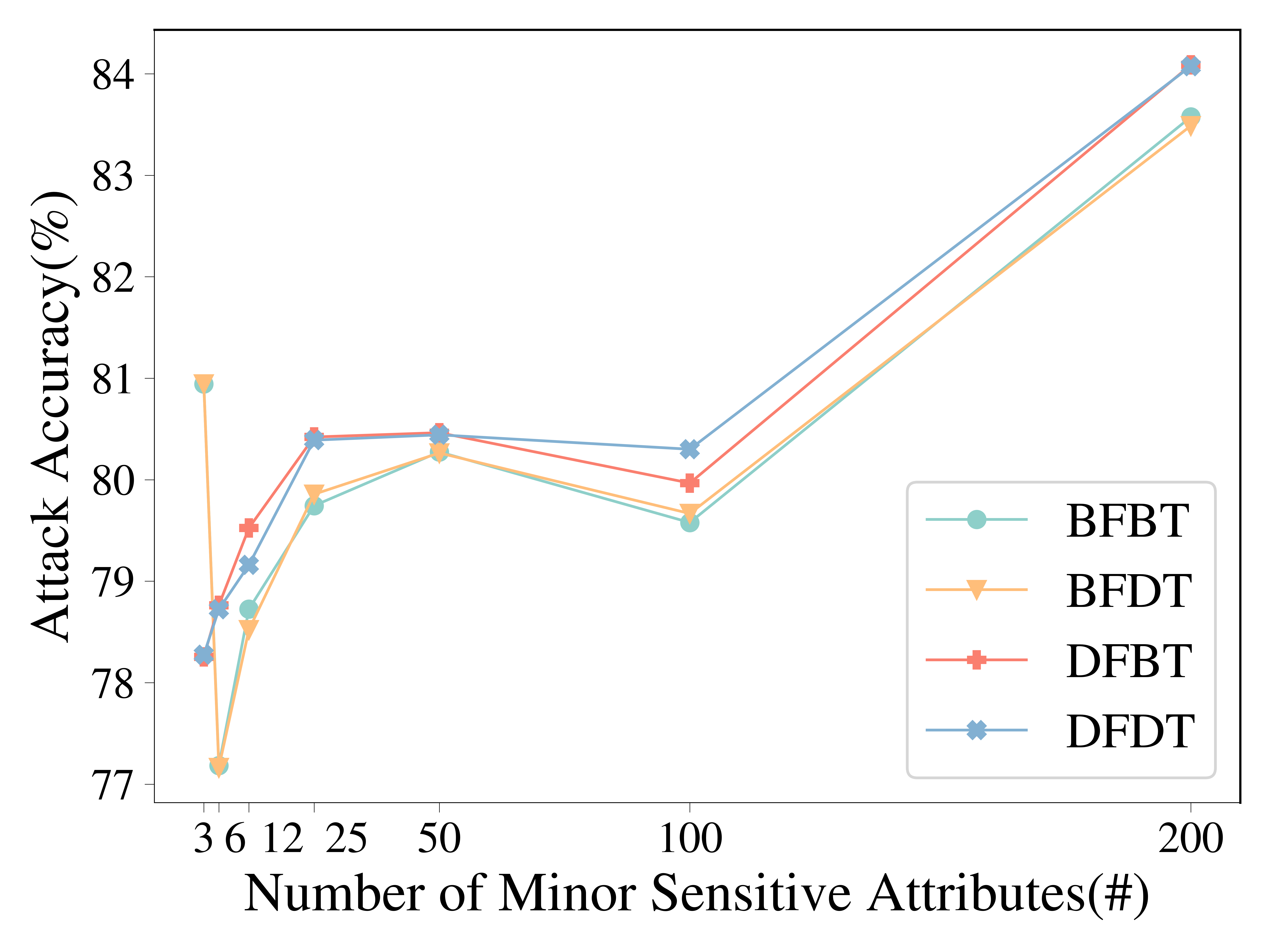
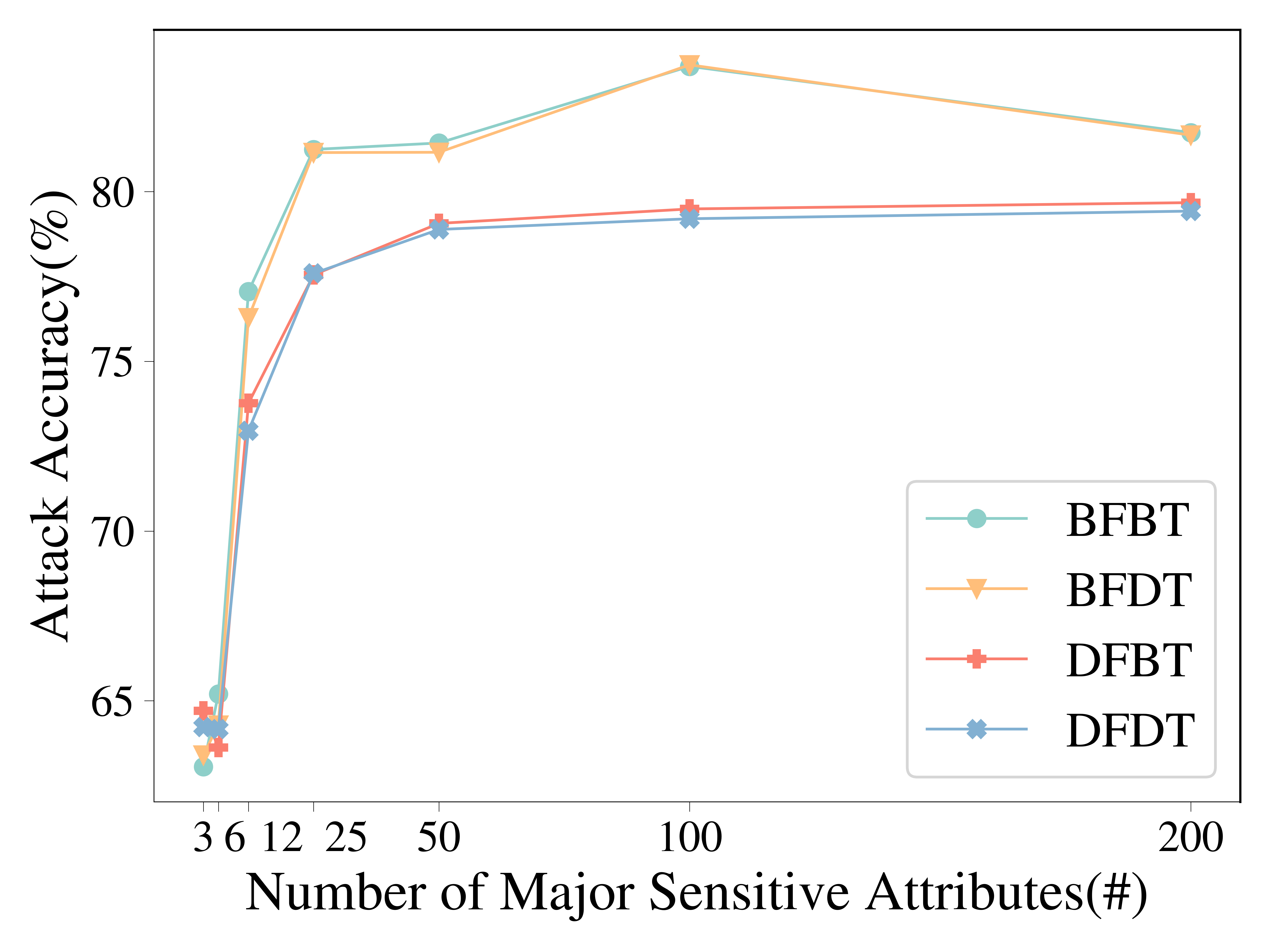
(a) Attack Accuracy of Multiple Sensitive Attributes

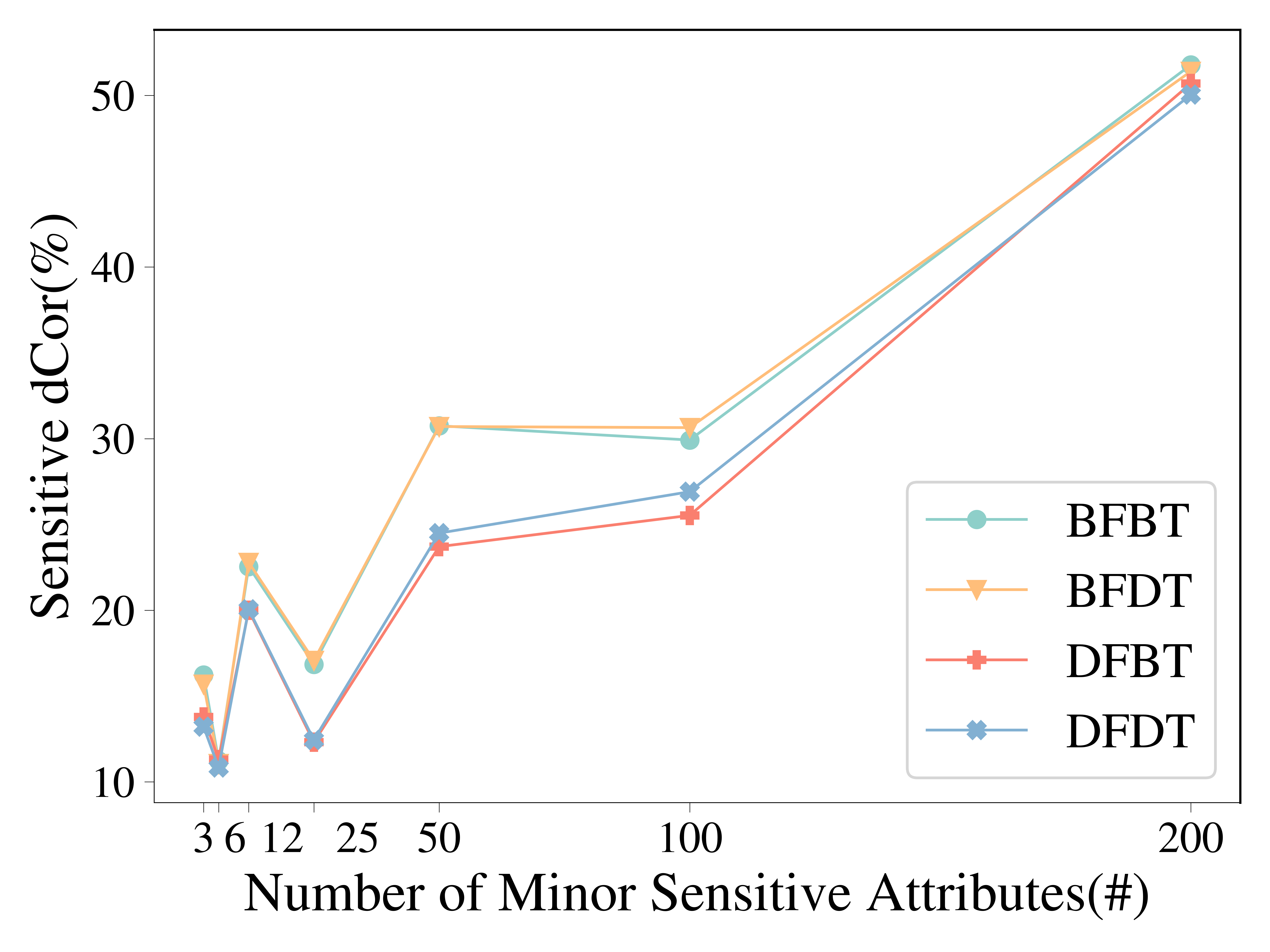
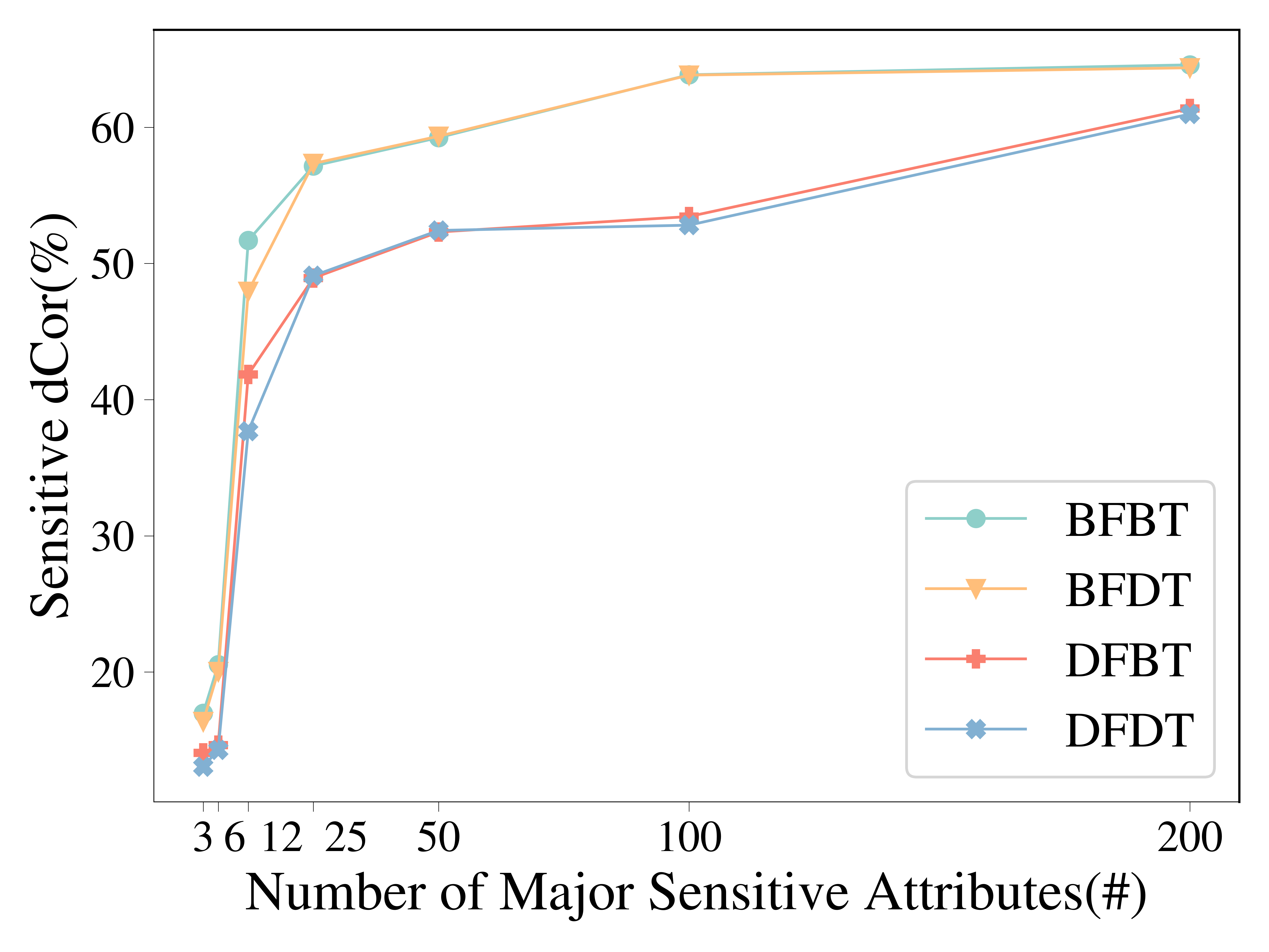
(b) Sensitive Correlation of Multiple Sensitive Attributes

Figure 6. Coefficient Impact of Utility and Fairness

From Figure 6, we observe similar patterns in the previous experiments. E.g, the performances of BFBT and BFDT pairs are close while the DFBT and DFDT pairs are close; and the not stable performances in fewer label cases may be the main reason why there are some turning points. The more interesting phenomenon is the performances of all pairs of the minor sensitive attributes are pretty close to each other, and their attack accuracy and sensitive correlation increase rapidly after collecting more sensitive labels, but the performances of all pairs of the major increase dramatically at the fewer label situations and seem stabilized to some points. Its sensitive correlation is higher than the minor but the attack accuracy is much lower. We leave the deeper investigation of this inverse fact as the future work.

C.4. Parameter Studies

The parameter studies have been discussed in the experimental section. Please note different colors represent for different coefficients, i.e., the green line denotes $\lambda_{2}$ and the red and blue lines denote $\lambda_{3}$ and $\lambda_{4}$, respectively. Different types of lines represent for different GNN variants, i.e., the straight line denotes GCN and the dotted line with larger intervals and the dotted line with smaller intervals denote GraphSAGE and GIN, respectively.

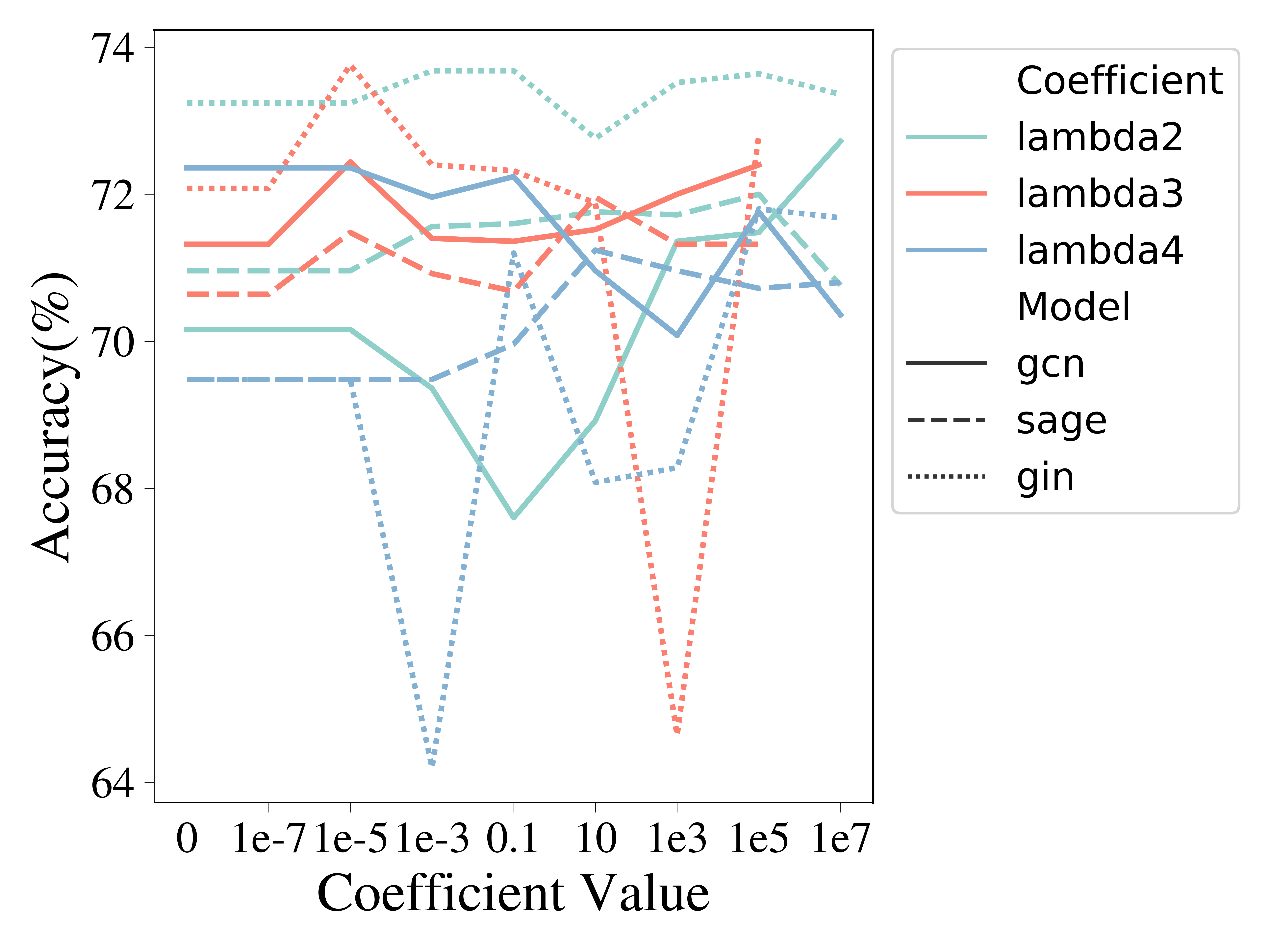
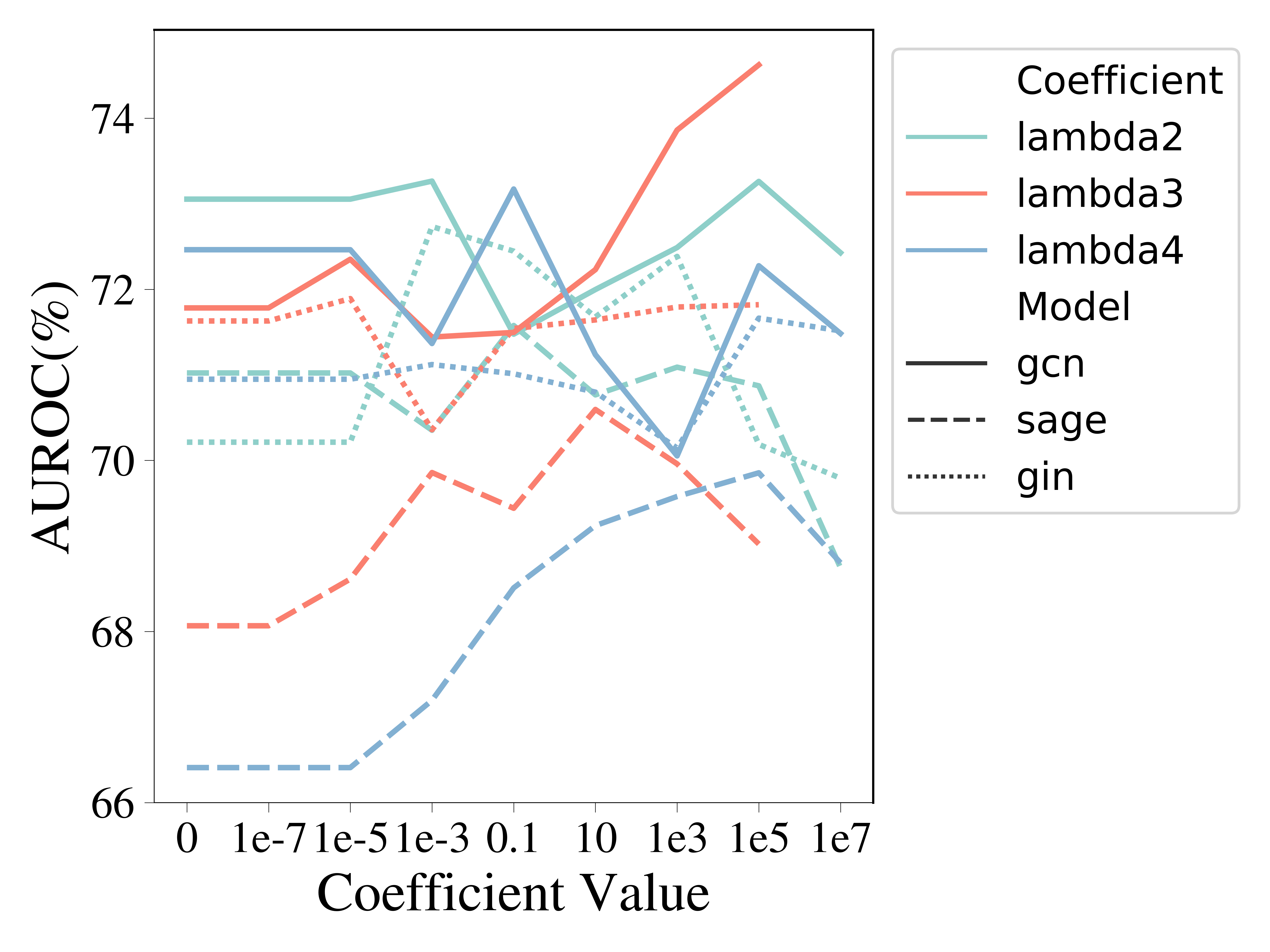
(a) Utility Performance of Node Classification

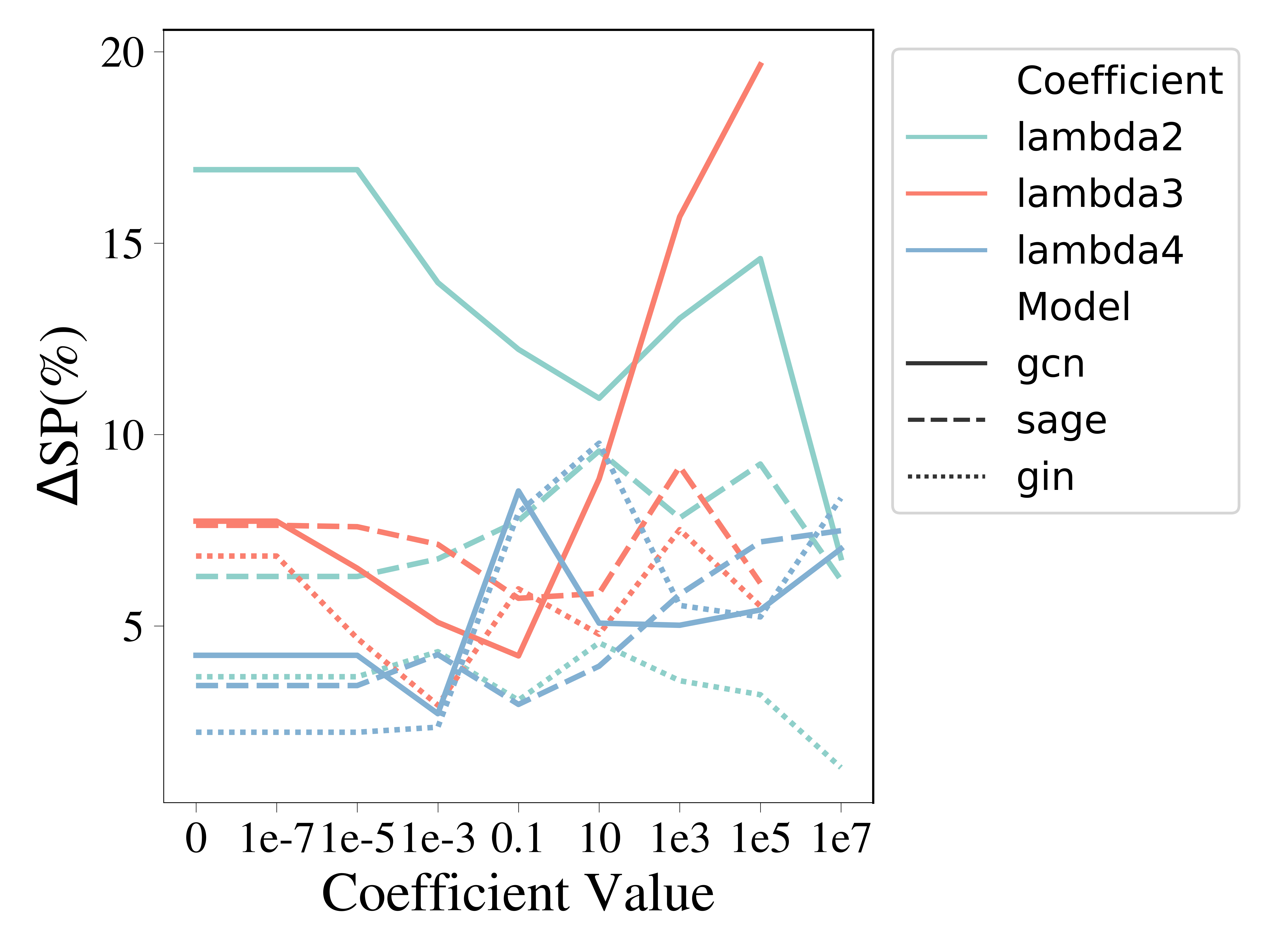
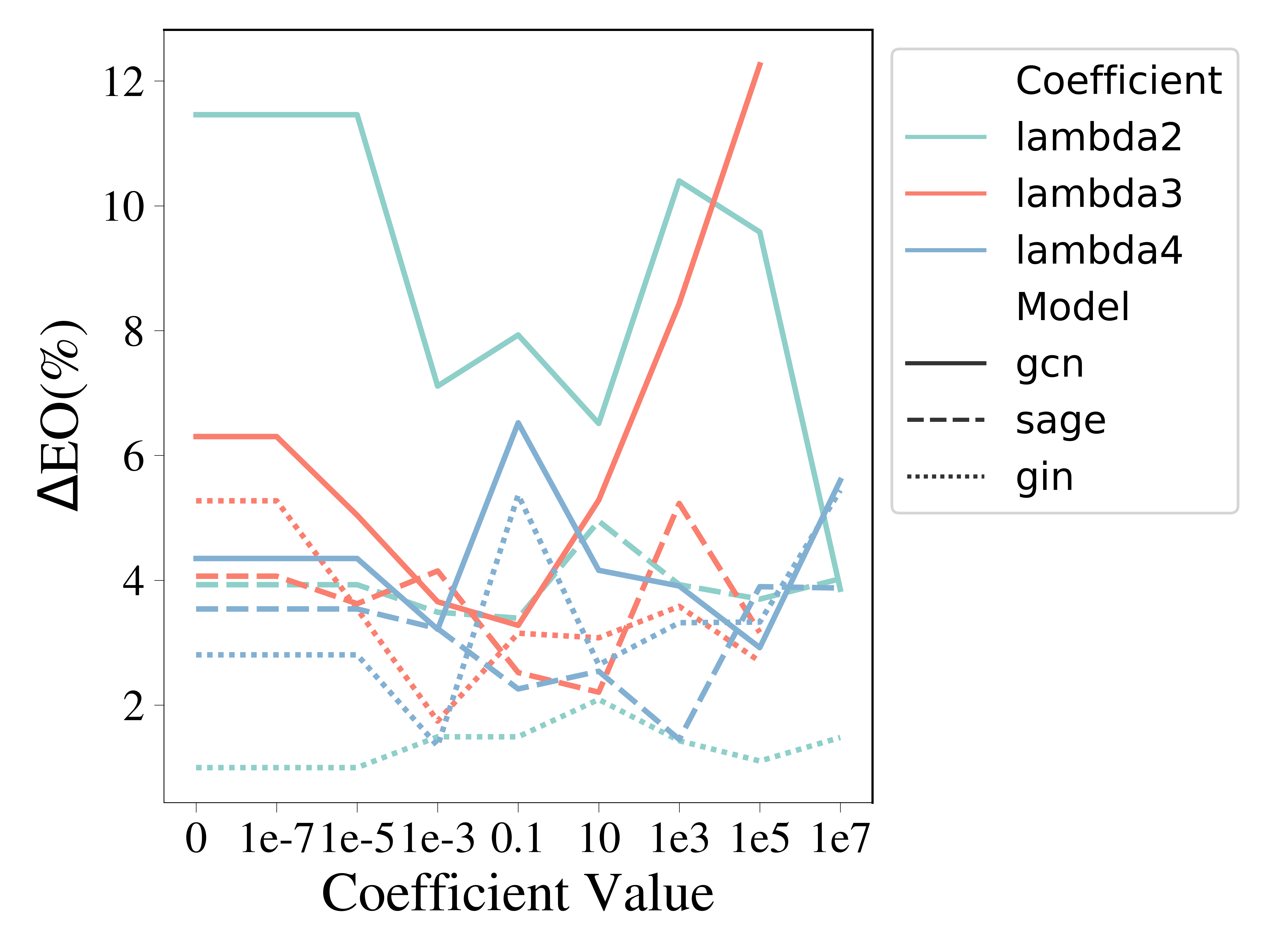
(b) Fairness Performance of Node Classification

Figure 7. Coefficient Impact of Utility and Fairness

References

- (1)
- Agarwal et al. (2021) Chirag Agarwal, Himabindu Lakkaraju, and Marinka Zitnik. 2021. Towards a unified framework for fair and stable graph representation learning. In Proceedings of the Thirty-Seventh Conference on Uncertainty in Artificial Intelligence (Proceedings of Machine Learning Research, Vol. 161). PMLR, 2114–2124. https://proceedings.mlr.press/v161/agarwal21b.html
- Akiba et al. (2019) Takuya Akiba, Shotaro Sano, Toshihiko Yanase, Takeru Ohta, and Masanori Koyama. 2019. Optuna: A Next-Generation Hyperparameter Optimization Framework. In Proceedings of the 25th ACM SIGKDD International Conference on Knowledge Discovery and Data Mining (Anchorage, AK, USA) (KDD ’19). Association for Computing Machinery, New York, NY, USA, 2623–2631. https://doi.org/10.1145/3292500.3330701
- Belghazi et al. (2018) Mohamed Ishmael Belghazi, Aristide Baratin, Sai Rajeshwar, Sherjil Ozair, Yoshua Bengio, Aaron Courville, and Devon Hjelm. 2018. Mutual Information Neural Estimation. In Proceedings of the 35th International Conference on Machine Learning (Proceedings of Machine Learning Research, Vol. 80). PMLR, 531–540. https://proceedings.mlr.press/v80/belghazi18a.html
- Beutel et al. (2017) Alex Beutel, Jilin Chen, Zhe Zhao, and Ed H. Chi. 2017. Data Decisions and Theoretical Implications when Adversarially Learning Fair Representations. arXiv:1707.00075 [cs.LG]
- Bose and Hamilton (2019) Avishek Joey Bose and William Hamilton. 2019. Compositional Fairness Constraints for Graph Embeddings. (2019).
- Chang and Shokri (2021) H. Chang and R. Shokri. 2021. On the Privacy Risks of Algorithmic Fairness. In 2021 IEEE European Symposium on Security and Privacy (EuroS&P). IEEE Computer Society, Los Alamitos, CA, USA, 292–303. https://doi.org/10.1109/EuroSP51992.2021.00028
- Chen et al. (2022) Canyu Chen, Yueqing Liang, Xiongxiao Xu, Shangyu Xie, Yuan Hong, and Kai Shu. 2022. When Fairness Meets Privacy: Fair Classification with Semi-Private Sensitive Attributes. In Workshop on Trustworthy and Socially Responsible Machine Learning, NeurIPS 2022.
- Cho et al. (2020) Jaewoong Cho, Gyeongjo Hwang, and Changho Suh. 2020. A Fair Classifier Using Mutual Information. In 2020 IEEE International Symposium on Information Theory (ISIT) (Los Angeles, CA, USA). IEEE Press, 2521–2526. https://doi.org/10.1109/ISIT44484.2020.9174293
- Dai and Wang (2021) Enyan Dai and Suhang Wang. 2021. Say No to the Discrimination: Learning Fair Graph Neural Networks with Limited Sensitive Attribute Information. In Proceedings of the 14th ACM International Conference on Web Search and Data Mining. 680–688.
- Dai and Wang (2022) Enyan Dai and Suhang Wang. 2022. Learning Fair Graph Neural Networks with Limited and Private Sensitive Attribute Information. IEEE Transactions on Knowledge and Data Engineering (2022), 1–14. https://doi.org/10.1109/TKDE.2022.3197554
- de Oliveira et al. (2023) Anderson Santana de Oliveira, Caelin Kaplan, Khawla Mallat, and Tanmay Chakraborty. 2023. An Empirical Analysis of Fairness Notions under Differential Privacy. arXiv:2302.02910 [cs.LG]
- Ding et al. (2020) Jiahao Ding, Xinyue Zhang, Xiaohuan Li, Junyi Wang, Rong Yu, and Miao Pan. 2020. Differentially private and fair classification via calibrated functional mechanism. In Proceedings of the AAAI Conference on Artificial Intelligence, Vol. 34. 622–629.
- Dong et al. (2022) Yushun Dong, Ninghao Liu, Brian Jalaian, and Jundong Li. 2022. Edits: Modeling and mitigating data bias for graph neural networks. In Proceedings of the ACM Web Conference 2022. 1259–1269.
- Dong et al. (5555) Y. Dong, J. Ma, S. Wang, C. Chen, and J. Li. 5555. Fairness in Graph Mining: A Survey. IEEE Transactions on Knowledge and Data Engineering 01 (apr 5555), 1–22. https://doi.org/10.1109/TKDE.2023.3265598
- Duddu et al. (2020) Vasisht Duddu, Antoine Boutet, and Virat Shejwalkar. 2020. Quantifying Privacy Leakage in Graph Embedding. In MobiQuitous 2020 - 17th EAI International Conference on Mobile and Ubiquitous Systems: Computing, Networking and Services. ACM. https://doi.org/10.1145/3448891.3448939
- Dwork et al. (2012) Cynthia Dwork, Moritz Hardt, Toniann Pitassi, Omer Reingold, and Richard Zemel. 2012. Fairness through Awareness. In Proceedings of the 3rd Innovations in Theoretical Computer Science Conference (Cambridge, Massachusetts) (ITCS ’12). Association for Computing Machinery, New York, NY, USA, 214–226. https://doi.org/10.1145/2090236.2090255
- Dwork et al. (2006) Cynthia Dwork, Frank McSherry, Kobbi Nissim, and Adam Smith. 2006. Calibrating Noise to Sensitivity in Private Data Analysis. In Theory of Cryptography. Springer Berlin Heidelberg, Berlin, Heidelberg, 265–284.
- Fan et al. (2019) Wenqi Fan, Yao Ma, Qing Li, Yuan He, Eric Zhao, Jiliang Tang, and Dawei Yin. 2019. Graph Neural Networks for Social Recommendation. In The World Wide Web Conference (San Francisco, CA, USA) (WWW ’19). Association for Computing Machinery, New York, NY, USA, 417–426. https://doi.org/10.1145/3308558.3313488
- Fey and Lenssen (2019) Matthias Fey and Jan E. Lenssen. 2019. Fast Graph Representation Learning with PyTorch Geometric. In ICLR Workshop on Representation Learning on Graphs and Manifolds.
- Hamberg (2008) Katarina Hamberg. 2008. Gender Bias in Medicine. Women’s Health 4, 3 (2008), 237–243. https://doi.org/10.2217/17455057.4.3.237 arXiv:https://doi.org/10.2217/17455057.4.3.237
- Hamilton et al. (2017) William L. Hamilton, Rex Ying, and Jure Leskovec. 2017. Inductive Representation Learning on Large Graphs. In NIPS.
- Hardt et al. (2016) Moritz Hardt, Eric Price, and Nathan Srebro. 2016. Equality of Opportunity in Supervised Learning. In Proceedings of the 30th International Conference on Neural Information Processing Systems (Barcelona, Spain) (NIPS’16). Curran Associates Inc., Red Hook, NY, USA, 3323–3331.
- Hou et al. (2022) Jie Hou, Xiufen Ye, Weixing Feng, Qiaosheng Zhang, Yatong Han, Yusong Yusong Liu, Yu Li, and Yufen Wei. 2022. Distance correlation application to gene co-expression network analysis. BMC Bioinformatics 23 (02 2022). https://doi.org/10.1186/s12859-022-04609-x
- Hu et al. (2022) Hui Hu, Lu Cheng, Jayden Parker Vap, and Mike Borowczak. 2022. Learning Privacy-Preserving Graph Convolutional Network with Partially Observed Sensitive Attributes. In Proceedings of the ACM Web Conference 2022. 3552–3561.
- Huang and Huo (2022) Cheng Huang and Xiaoming Huo. 2022. A Statistically and Numerically Efficient Independence Test Based on Random Projections and Distance Covariance. Frontiers in Applied Mathematics and Statistics 7 (2022). https://doi.org/10.3389/fams.2021.779841
- Huo and Székely (2016) Xiaoming Huo and Gábor J. Székely. 2016. Fast Computing for Distance Covariance. Technometrics 58, 4 (2016), 435–447. https://doi.org/10.1080/00401706.2015.1054435 arXiv:https://doi.org/10.1080/00401706.2015.1054435
- Jayaraman and Evans (2022) Bargav Jayaraman and David Evans. 2022. Are Attribute Inference Attacks Just Imputation?. In Proceedings of the 2022 ACM SIGSAC Conference on Computer and Communications Security (Los Angeles, CA, USA) (CCS ’22). Association for Computing Machinery, New York, NY, USA, 1569–1582. https://doi.org/10.1145/3548606.3560663
- Jiang et al. (2022) Zhimeng Jiang, Xiaotian Han, Chao Fan, Zirui Liu, Na Zou, Ali Mostafavi, and Xia Hu. 2022. FMP: Toward Fair Graph Message Passing against Topology Bias. arXiv:2202.04187 [cs.LG]
- Kamiran and Calders (2011) Faisal Kamiran and Toon Calders. 2011. Data Pre-Processing Techniques for Classification without Discrimination. Knowledge and Information Systems 33 (10 2011). https://doi.org/10.1007/s10115-011-0463-8
- Kingma and Ba (2015) Diederik P. Kingma and Jimmy Ba. 2015. Adam: A Method for Stochastic Optimization. In 3rd International Conference on Learning Representations, ICLR 2015, San Diego, CA, USA, May 7-9, 2015, Conference Track Proceedings. http://arxiv.org/abs/1412.6980
- Li et al. (2020) Kaiya Li, Guangchun Luo, Yang Ye, Wei Li, Shihao Ji, and Zhipeng Cai. 2020. Adversarial Privacy-Preserving Graph Embedding Against Inference Attack. IEEE Internet of Things Journal 8 (2020), 6904–6915.
- Li et al. (2022) Yang Li, Michael Purcell, Thierry Rakotoarivelo, David Smith, Thilina Ranbaduge, and Kee Siong Ng. 2022. Private Graph Data Release: A Survey. arXiv:2107.04245 [cs.CR]
- Liao et al. (2021) Peiyuan Liao, Han Zhao, Keyulu Xu, Tommi Jaakkola, Geoffrey J. Gordon, Stefanie Jegelka, and Ruslan Salakhutdinov. 2021. Information Obfuscation of Graph Neural Networks. In Proceedings of the 38th International Conference on Machine Learning (Proceedings of Machine Learning Research, Vol. 139). PMLR, 6600–6610. http://proceedings.mlr.press/v139/liao21a.html
- Louizos et al. (2017) Christos Louizos, Kevin Swersky, Yujia Li, Max Welling, and Richard Zemel. 2017. The Variational Fair Autoencoder. arXiv:1511.00830 [stat.ML]
- Masrour et al. (2020) Farzan Masrour, Tyler Wilson, Heng Yan, Pang-Ning Tan, and Abdol Esfahanian. 2020. Bursting the Filter Bubble: Fairness-Aware Network Link Prediction. Proceedings of the AAAI Conference on Artificial Intelligence 34, 01 (Apr. 2020), 841–848. https://doi.org/10.1609/aaai.v34i01.5429
- Oneto et al. (2020) Luca Oneto, Nicolò Navarin, and Michele Donini. 2020. Learning Deep Fair Graph Neural Networks. In 28th European Symposium on Artificial Neural Networks, Computational Intelligence and Machine Learning, ESANN 2020, Bruges, Belgium, October 2-4, 2020. 31–36. https://www.esann.org/sites/default/files/proceedings/2020/ES2020-75.pdf
- Paszke et al. (2019) Adam Paszke, Sam Gross, Francisco Massa, Adam Lerer, James Bradbury, Gregory Chanan, Trevor Killeen, Zeming Lin, Natalia Gimelshein, Luca Antiga, Alban Desmaison, Andreas Kopf, Edward Yang, Zachary DeVito, Martin Raison, Alykhan Tejani, Sasank Chilamkurthy, Benoit Steiner, Lu Fang, Junjie Bai, and Soumith Chintala. 2019. PyTorch: An Imperative Style, High-Performance Deep Learning Library. In Advances in Neural Information Processing Systems 32. Curran Associates, Inc., 8024–8035. http://papers.neurips.cc/paper/9015-pytorch-an-imperative-style-high-performance-deep-learning-library.pdf
- Pujol et al. (2020) David Pujol, Ryan McKenna, Satya Kuppam, Michael Hay, Ashwin Machanavajjhala, and Gerome Miklau. 2020. Fair Decision Making Using Privacy-Protected Data. In Proceedings of the 2020 Conference on Fairness, Accountability, and Transparency (Barcelona, Spain) (FAT* ’20). Association for Computing Machinery, New York, NY, USA, 189–199. https://doi.org/10.1145/3351095.3372872
- Rahman et al. (2019) Tahleen Rahman, Bartlomiej Surma, Michael Backes, and Yang Zhang. 2019. Fairwalk: Towards Fair Graph Embedding. In Proceedings of the Twenty-Eighth International Joint Conference on Artificial Intelligence, IJCAI-19. International Joint Conferences on Artificial Intelligence Organization, 3289–3295. https://doi.org/10.24963/ijcai.2019/456
- Roh et al. (2020) Yuji Roh, Kangwook Lee, Steven Euijong Whang, and Changho Suh. 2020. FR-Train: A Mutual Information-Based Approach to Fair and Robust Training. In Proceedings of the 37th International Conference on Machine Learning (ICML’20). JMLR.org, Article 754, 11 pages.
- SKEEM and LOWENKAMP (2016) JENNIFER L. SKEEM and CHRISTOPHER T. LOWENKAMP. 2016. RISK, RACE, AND RECIDIVISM: PREDICTIVE BIAS AND DISPARATE IMPACT*. Criminology 54, 4 (2016), 680–712. https://doi.org/10.1111/1745-9125.12123 arXiv:https://onlinelibrary.wiley.com/doi/pdf/10.1111/1745-9125.12123
- Song and Ermon (2020) Jiaming Song and Stefano Ermon. 2020. Understanding the Limitations of Variational Mutual Information Estimators. (2020).
- Spinelli et al. (2021) Indro Spinelli, Simone Scardapane, Amir Hussain, and Aurelio Uncini. 2021. FairDrop: Biased Edge Dropout for Enhancing Fairness in Graph Representation Learning. IEEE Transactions on Artificial Intelligence (2021), 1–1. https://doi.org/10.1109/TAI.2021.3133818
- Staerman et al. (2021) Guillaume Staerman, Pierre Laforgue, Pavlo Mozharovskyi, and Florence d’Alché Buc. 2021. When OT meets MoM: Robust estimation of Wasserstein Distance. In Proceedings of The 24th International Conference on Artificial Intelligence and Statistics (Proceedings of Machine Learning Research, Vol. 130). PMLR, 136–144. https://proceedings.mlr.press/v130/staerman21a.html
- Suresh and Guttag (2021) Harini Suresh and John Guttag. 2021. A Framework for Understanding Sources of Harm throughout the Machine Learning Life Cycle. In Equity and Access in Algorithms, Mechanisms, and Optimization. ACM. https://doi.org/10.1145/3465416.3483305
- Székely et al. (2007) Gábor J. Székely, Maria L. Rizzo, and Nail K. Bakirov. 2007. Measuring and testing dependence by correlation of distances. The Annals of Statistics 35, 6 (2007), 2769 – 2794. https://doi.org/10.1214/009053607000000505
- Székely et al. (2007) Gábor J. Székely, Maria L. Rizzo, and Nail K. Bakirov. 2007. Measuring and Testing Dependence by Correlation of Distances. The Annals of Statistics 35, 6 (2007), 2769–2794. http://www.jstor.org/stable/25464608
- van der Maaten and Hinton (2008) Laurens van der Maaten and Geoffrey Hinton. 2008. Visualizing Data using t-SNE. Journal of Machine Learning Research 9, 86 (2008), 2579–2605. http://jmlr.org/papers/v9/vandermaaten08a.html
- Villani (2003) C. Villani. 2003. Topics in Optimal Transportation Theory. 58 (01 2003). https://doi.org/10.1090/gsm/058
- Wang et al. (2021) Binghui Wang, Jiayi Guo, Ang Li, Yiran Chen, and Hai Li. 2021. Privacy-Preserving Representation Learning on Graphs: A Mutual Information Perspective. In Proceedings of the 27th ACM SIGKDD Conference on Knowledge Discovery and Data Mining (Virtual Event, Singapore) (KDD ’21). Association for Computing Machinery, New York, NY, USA, 1667–1676. https://doi.org/10.1145/3447548.3467273
- Wang et al. (2019) Hao Wang, Berk Ustun, and Flavio Calmon. 2019. Repairing without Retraining: Avoiding Disparate Impact with Counterfactual Distributions. In Proceedings of the 36th International Conference on Machine Learning (Proceedings of Machine Learning Research, Vol. 97). PMLR, 6618–6627. https://proceedings.mlr.press/v97/wang19l.html
- Wang et al. (2022) Yu Wang, Yuying Zhao, Yushun Dong, Huiyuan Chen, Jundong Li, and Tyler Derr. 2022. Improving Fairness in Graph Neural Networks via Mitigating Sensitive Attribute Leakage. In SIGKDD.
- Weisfeiler and Lehman (1968) Boris Weisfeiler and AA Lehman. 1968. A reduction of a graph to a canonical form and an algebra arising during this reduction.. In Nauchno-Technicheskaya Informatsia, Vol. 2(9). 12–16.
- Wu et al. (2020) Zonghan Wu, Shirui Pan, Fengwen Chen, Guodong Long, Chengqi Zhang, and Philip S Yu. 2020. A comprehensive survey on graph neural networks. IEEE Transactions on Neural Networks and Learning Systems (mar 2020). https://arxiv.org/pdf/1901.00596.pdf
- Xu et al. (2019) Keyulu Xu, Weihua Hu, Jure Leskovec, and Stefanie Jegelka. 2019. How Powerful are Graph Neural Networks?. In International Conference on Learning Representations. https://openreview.net/forum?id=ryGs6iA5Km
- Yang et al. (2022) Zhiju Yang, Weiping Pei, Monchu Chen, and Chuan Yue. 2022. WTAGRAPH: Web Tracking and Advertising Detection using Graph Neural Networks. In 2022 IEEE Symposium on Security and Privacy (SP). 1540–1557. https://doi.org/10.1109/SP46214.2022.9833670
- Zafar et al. (2017) Muhammad Bilal Zafar, Isabel Valera, Manuel Gomez Rodriguez, and Krishna P. Gummadi. 2017. Fairness Beyond Disparate Treatment and Disparate Impact: Learning Classification without Disparate Mistreatment. In Proceedings of the 26th International Conference on World Wide Web (Perth, Australia) (WWW ’17). International World Wide Web Conferences Steering Committee, Republic and Canton of Geneva, CHE, 1171–1180. https://doi.org/10.1145/3038912.3052660
- Zhang et al. (2018) Brian Hu Zhang, Blake Lemoine, and Margaret Mitchell. 2018. Mitigating Unwanted Biases with Adversarial Learning. In Proceedings of the 2018 AAAI/ACM Conference on AI, Ethics, and Society (New Orleans, LA, USA) (AIES ’18). Association for Computing Machinery, New York, NY, USA, 335–340. https://doi.org/10.1145/3278721.3278779
- Zhang et al. (2023) He Zhang, Xingliang Yuan, Quoc Viet Hung Nguyen, and Shirui Pan. 2023. On the Interaction between Node Fairness and Edge Privacy in Graph Neural Networks. arXiv:2301.12951 [cs.LG]
- Zhao et al. (2022) Tianxiang Zhao, Enyan Dai, Kai Shu, and Suhang Wang. 2022. Towards Fair Classifiers Without Sensitive Attributes: Exploring Biases in Related Features. In Proceedings of the Fifteenth ACM International Conference on Web Search and Data Mining (Virtual Event, AZ, USA) (WSDM ’22). Association for Computing Machinery, New York, NY, USA, 1433–1442. https://doi.org/10.1145/3488560.3498493
- Zhu and Wang (2022) Huaisheng Zhu and Suhang Wang. 2022. Learning Fair Models without Sensitive Attributes: A Generative Approach. arXiv:2203.16413 [cs.LG]