Sublattice-selective percolation on bipartite planar lattices

Abstract

In conventional site percolation, all lattice sites are occupied with the same probability. For a bipartite lattice, sublattice-selective percolation instead involves two independent occupation probabilities, depending on the sublattice to which a given site belongs. Here, we determine the corresponding phase diagram for the two-dimensional square and Lieb lattices from quantifying the parameter regime where a percolating cluster persists for sublattice-selective percolation. For this purpose, we present an adapted Newman–Ziff algorithm. We also consider the critical exponents at the percolation transition, confirming previous Monte Carlo and renormalization-group findings that suggest sublattice-selective percolation to belong to the same universality class as conventional site percolation. To further strengthen this conclusion, we finally treat sublattice-selective percolation on the Bethe lattice (infinite Cayley tree) by an exact solution.

I Introduction

Percolation provides a remarkably simple route to nontrivial critical phenomena that has a broad range of applications in many fields of science and engineering Flory (1941); Stauffer and Aharony (2018). In its most basic formulation, one considers an infinite periodic lattice, occupying each lattice site independently with equal probability $p$. The occupied sites from contiguous clusters of connected lattice sites, which turn out to exhibit several interesting properties. In particular, an infinite, spanning (percolating) cluster of connected occupied sites emerges for sufficiently large values of $p$ beyond a particular threshold value $p_{c}$. For example, considering a two-dimensional square lattice, the site percolation threshold $p^{\mathrm{sq}}_{c}=0.592746...$ Lee (2008); Jacobsen (2015) is known from computational studies to rather high accuracy – the exact value being however unknown to date. In the vicinity of the percolation threshold, various characteristics of the cluster distribution exhibit non-trivial scaling behavior: For $p\gtrsim p_{c}$, the strength $P$ of the percolating cluster, i.e., the probability that a given site belongs to the percolating cluster, increases with $p$ by an asymptotic power law,

$$P\propto(p-p_{c})^{\beta},$$ (1)

resembling the scaling behavior of an order parameter near a thermal ordering phase transition. Upon approaching $p_{c}$, the correlation length $\xi$, defined as the mean distance between two sites belonging to the same finite cluster, increases as

$$\xi\propto|p-p_{c}|^{-\nu},$$ (2)

and the mean number of sites of a finite cluster $S$ as

$$S\propto|p-p_{c}|^{-\gamma},$$ (3)

corresponding to the order parameter susceptibility in thermal ordering transitions. The scaling exponents describe the critical behavior at the percolation transition of the above state functions and are considered universal in the sense that within a given dimension $d$ they do not depend on details of the lattice structure (e.g., square or triangluar in $d=2$) or the kind of percolation problem considered (site, bond or also in the continuum) Stauffer and Aharony (2018). For $d=2$ the exponents are known as $\beta=5/36=0.13\bar{8}$, $\nu=4/3$, and $\gamma=43/18=2.3\bar{8}$, respectively Smirnov and Werner (2001); Stauffer and Aharony (2018). Furthermore, at the percolation threshold, the infinite cluster has a fractal dimension $d_{f}=d-\beta/\nu$, e.g., $d_{f}=91/48=1.8958\bar{3}$ for the two-dimensional case.

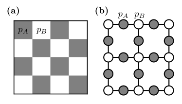
Figure 1: Illustration of the square (a) and Lieb lattice (b). Sites from sublattice $A$ and $B$ are shown in grey (white). The square lattice is shown as a checkerboard, while the nearest neighbour bonds of the Lieb lattice are shown explicitly.

In physical systems the lattice sites considered above may represent objects such as atoms in a solid state crystal, an empty site being related to a defect, e.g., an impurity atom. In many condensed matter systems, the underlying lattice structure shows further characteristics, such as being bipartite, i.e., the total set of lattice sites can be decomposed into two disjoint sublattices, denoted $A$ and $B$ in the following, with nearest neighbor sites always belonging to different sublattices (cf. Fig. 1 for two examples). If, for example in a binary system, the objects occupying the $A$ and $B$ sublattice are of different species, it becomes feasible that the susceptibility to a defect differs on the $A$ and $B$ sublattice. In the context of site percolation, such a circumstance can be described by assigning two different occupation probabilities $p_{A}$ and $p_{B}$ to sites from sublattice $A$ and $B$, respectively. Such sublattice-selective percolation was introduced by Scholl and Binder in Ref. Scholl and Binder (1980), motivated by the properties of diluted magnetic compounds, with a special focus towards experimental findings in three-dimensional spinel structures. For the latter case, they performed Monte Carlo simulations to extract the phase diagram in terms of percolating vs. non-percolating regimes of parameters $(p_{A},p_{B})$ and provide numerical evidence that the critical exponents of sublattice-selective percolation are those of the universality class for conventional site percolation (where $p_{A}=p_{B}$). Ref. Scholl and Binder (1980) also considered several other lattice structures, both in three and two dimensions, focusing on the extreme case where one sublattice is fully occupied, e.g., $p_{B}=1$. In various cases, the critical value $p_{A,c}$ for $p_{A}$ can then be expressed in terms of the percolation threshold of certain related conventional percolation problems. For example, for a square lattice with $p_{A}=1$, the threshold value $p_{A,c}$ equals the site percolation threshold for a square lattice with next-nearest neighbor connectivity. Using the concept of matching lattices, this value can furthermore be shown to be equal to $1-p^{\mathrm{sq}}_{c}=0.407253...$ Sykes and Essam (1964). For $p_{B}=1$, the percolation threshold for $p_{A}$ thus falls below the value of $p^{\mathrm{sq}}_{c}$ – as expected, since half of the lattice is already occupied for $p_{B}=1$. Due to the equivalence between the two sublattices of the square lattice, the problem is symmetric under the exchange of $p_{A}$ and $p_{B}$ in this case. In particular, $p_{B,c}=1-p^{\mathrm{sq}}_{c}$ along the line $p_{A}=1$, and along the symmetric line $p_{A}=p_{B}$, the critical value $p^{\mathrm{sq}}_{c}$ is recovered. A quantification of the full boundary line in the $(p_{A},p_{B})$-plane of the percolating regime was however not performed in Ref. Scholl and Binder (1980) for the basic square lattice case. Later, approximate renormalization-group (RG) calculations were used to estimate this boundary line Idogaki and Uryû (1982) and to address the question of universality (the method was furthermore employed to study sublattice-selective percolation on other lattices and sublattice geometries Idogaki and Uryu (1982); Idogaki and Uryû (1983)). However, while the RG approach finds that sublattice-selective percolation is indeed controlled by the same fixed point as the uniform case, its numerical accuracy is limited. For example, in the uniform case a best estimate of 0.610 was obtained for $p^{\mathrm{sq}}_{c}$ Idogaki and Uryû (1982). Related work, using a decoupling approximation for an effective field theory of the Ising model with sublattice-selective depletion yields results of similar accuracy Idogaki et al. (1995); Ueda et al. (2000). Since those early works on sublattice-selective percolation, several methodological advances have been achieved, such as the Newman–Ziff algorithm Newman and Ziff (2000, 2001), which allows for efficient high-accuracy numerical studies of conventional lattice-based percolation problems. It is thus feasible now to also perform a systematic and accurate exploration of sublattice-selective percolation on basic planar lattices, such as the square lattice using such advanced algorithms.

Here, we perform such an analysis using an adapted version of the Newman–Ziff algorithm Newman and Ziff (2000, 2001), which we detail further below. This algorithm allows for efficient Monte Carlo studies of the phase diagram, like the original algorithm does for conventional percolation problems on periodic lattices. In addition to the square lattice, we examine the case of the planar Lieb lattice, which is also bipartite, and for which conventional site-percolation has been considered recently Oliveira et al. (2021). This lattice, which is of interest in the context of flat band physics, ferrimagnetism and topological states, is a decorated square lattice and bipartite, cf. Fig. 1. However, in contrast to the square lattice, the two sublattices $A$ and $B$ of the Lieb lattice are not equivalent, and the phase diagram of sublattice-selective percolation is non-symmetric in the $(p_{A},p_{B})$-plane. Furthermore, we use finite-size scaling in order to estimate the critical exponents for sublattice-selective percolation on the square lattice. Our results support previous conclusions Scholl and Binder (1980); Idogaki and Uryû (1982) regarding the universal properties.

The remainder of this article is organized as follows: In Sec. II, we introduce an adapted Newman–Ziff algorithm for efficient computational studies of sublattice-selective percolation. Then, we report our results for the square and Lieb lattice in Secs. III and  IV, respectively. Finally, in Sec. V, we study sublattice-selective percolation on the Bethe lattice, which in various aspects corresponds to infinite dimension, $d=\infty$, for coordination numbers $z\geq 3$, cf. Fig. 2 for an illustration for $z=3$. We determine the critical exponents analytically for the cases $z=2$ (corresponding to the chain, $d=1$) and $z=3$, thereby demonstrating explicitly the anticipated universality. Our final conclusions are given in Sec. VI.

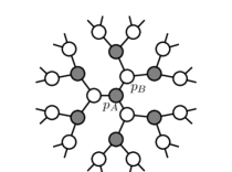
Figure 2: Illustration of the Bethe lattice for $z=3$. Sites from sublattice $A$ and $B$ are shown in grey (white). Note that for the infinite lattice, all sites are in fact topologically equivalent.

II Bipartite Newman–Ziff Algorithm

The Newman–Ziff algorithm Newman and Ziff (2000, 2001) performs Monte Carlo sampling of the percolation problem on finite lattices of linear size $L$ and with $N\propto L^{2}$ lattice sites in two dimensions. For a given system size one measures appropriate finite-size estimators $Q_{L}$ for any of the state functions $Q$, such as the quantities $P$, $\xi$ and $S$ introduced above. In the following, we consider finite systems with periodic boundaries, and a cluster is defined to be percolating if it completely wraps around in either direction. The main idea behind the Newman–Ziff algorithm can be loosely described as first calculating a given state function $Q_{L}$ in the microcanonical ensemble and then transforming to the canonical ensemble. In the microcanonical ensemble for a bipartite lattice, the state function is a function $Q_{L}(n_{A},n_{B})$ of the number of occupied sites $n_{A}$ and $n_{B}$ for each sublattice, while in the canonical ensemble it is a function of the probabilities, $Q_{L}(p_{A},p_{B})$. This is an analogy to thermodynamics, where $n_{A}$ corresponds to the energy of the system and $p_{A}$ corresponds to the temperature.

To explore the phase diagram, we take cuts for fixed values of $p_{B}$, which means populating each site on the $B$ sublattice with probability $p_{B}$ and then successively and randomly adding sites to the $A$ sublattice until it is full, thus calculating $Q_{L}(n_{A},p_{B})$ for all values of $n_{A}$. Then the transformation to the canonical ensemble, i.e., $Q_{L}(n_{A},p_{B})\rightarrow Q_{L}(p_{A},p_{B})$, is performed for the $A$ sublattice only. For a given value of $p_{A}$, the probability $B(N_{A},n_{A},p_{A})$ that there are exactly $n_{A}$ sites occupied from the total number of $N_{A}$ sites of the $A$ sublattice is given by

$$B(N_{A},n_{A},p_{A})=\binom{N_{A}}{n_{A}}p_{A}^{n_{A}}(1-p_{A})^{N_{A}-n_{A}},$$ (4)

since choosing the occupied sites is a Bernoulli process. Weighing the (with respect to the $A$ sublattice) microcanonical state function $Q_{L}(n_{A},p_{B})$ by the probability in Eq. (4) and summing over all values of $n_{A}$ gives the canonical state function $Q_{L}(p_{A},p_{B})$,

$$Q_{L}(p_{A},p_{B})=\sum_{n_{A}=0}^{N_{A}}B(N_{A},n_{A},p_{A})Q_{L}(n_{A},p_{B}),$$ (5)

which is essentially a convolution with the binomial distribution. This transformation is again analogous to thermodynamics, where the transformation is performed via the Boltzmann distribution instead of the binomial distribution.

The efficiency of the Newman–Ziff algorithm derives from the fact that the number of samples for $p_{A}$ is only limited by the cost of the transformation in Eq. (5) and that this transformation is linear in the state function $Q_{L}$. Hence, only the average of the microcanonical state function after many Monte Carlo steps has to be transformed explicitly,

$$\langle Q_{L}(p_{A},p_{B})\rangle=\sum_{n_{A}=0}^{N_{A}}B(N_{A},n_{A},p_{A})\langle Q_{L}(n_{A},p_{B})\rangle.$$ (6)

The algorithm thus consists of three main steps. Firstly, every site on the $B$ sublattice is occupied with a given probability $p_{B}$, as seen in the example of Fig. 3(a). Since the lattice is bipartite, there are no clusters of size greater that single sites at this point.

Secondly, sites on the $A$ sublattice are randomly occupied according to a random permutation of the sublattice indices. Every time a site is occupied one checks each nearest neighbour one by one, and if the neighbour is occupied and belongs to a different cluster these are merged using a union–find routine, as in the original Newman–Ziff algorithm. Every time a site is newly occupied, the state functions $Q_{L}(n_{A},p_{B})$ are added to the mean $\langle Q_{L}(n_{A},p_{B})\rangle$. In Fig. 3(b), the state in which the cluster first percolates (with periodic boundary conditions) is shown. In Fig. 3(c) , the lattice is shown after adding 75 further occupied sites, and only a few small clusters besides the percolating cluster remain.

Thirdly, all the state functions are transformed according to Eq. (6). The binomial coefficients are computed recursively Newman and Ziff (2001), as

$$B(N_{A},n_{A},p_{A})=\begin{dcases}B(N_{A},n_{A}-1,p_{A})\frac{N_{A}-n_{A}+1}{n_{A}}\frac{p_{A}}{\bar{p}_{A}}\\ B(N_{A},n_{A}+1,p_{A})\frac{n_{A}+1}{N_{A}-n_{A}}\frac{\bar{p}_{A}}{p_{A}}\end{dcases},$$

for $n_{A}>p_{A}N_{A}$ and $n_{A}<p_{A}N_{A}$, respectively, with $\bar{p}_{A}=1-p_{A}$. In practice, $B(N_{A},n_{A},p_{A})$ is negligible for many values of $n_{A}$, so only seven standard deviations $\sqrt{p_{A}(1-p_{A})N_{A}}$ around the maximum value $p_{A}N_{A}$ are actually calculated, which only excludes $B(N_{A},n_{A},p_{A})\lesssim 10^{-10}$.

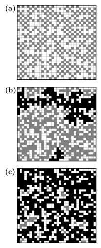
Figure 3: Illustration of the sublattice-selective percolation process for an $L=32$ square lattice and periodic boundary conditions. Occupied (empty) sites are shown in grey (white), and the percolating cluster in black. Starting from a random occupation of the $B$ sublattice sites with probability $p_{B}=0.7$, the $A$ sublattice is empty in (a), filled by $n_{A}=225$ sites in (b) and $n_{A}=300$ sites in (c).

In the actual implementation, the lattice is represented by an integer array of size $N$. If a site is occupied, it is part of a tree, and each tree corresponds to one cluster. A cluster of size $s$ has one root, which has an array entry of value $-s$, while the other sites of the cluster have pointers (indices of the array) which eventually lead to the root. The idea behind the aforementioned union–find algorithm is that the union operation merges two trees and the find operation returns the root of a given occupied site. So if there are two neighbouring occupied sites on the lattice, the roots can be compared via find and if the roots are different, the trees will be merged via union. Figure 4 shows an example of this procedure. The light grey site in Fig. 4(a) has been newly added, making it a tree just consisting of a root. Next, it is merged with the right cluster in Fig. 4(b), making a larger cluster of size $s=5$. In the next step in Fig. 4(c), the roots of the light grey site and the site to the left of it are compared via the find operation, and the roots are at different lattice sites. Thus, the union operation is invoked, and the root of the left tree then points to the root of the right tree and the cluster sizes are added. Now every site in the cluster returns the same root with find. There are a couple of methods to make this procedure more efficient: Firstly, the so called path compression is the idea that the find operation is most efficient when the path to the root involves as few pointers as possible. So every time the find operation follows a path from some site to the root, all the pointers on its way are set to point directly to the root – in practice this makes the trees never deeper than a few generations. Secondly, a smaller cluster is always appended to a bigger one. The find operation for the cluster that is appended takes one step longer, hence by appending the smaller cluster, the average number of steps is again minimized.

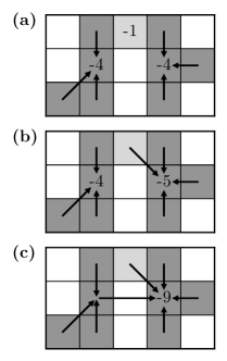
Figure 4: Example of adding a newly occupied site on a square lattice. Grey sites are occupied and the light grey site is newly occupied. The roots are marked by negative numbers and the arrows symbolize pointers.

In terms of computational complexity, using approaches based on alternative methods, such as the Hoshen–Kopelman algorithm Hoshen and Kopelman (1976), one would have to build all clusters for every value of $p_{A}$ from scratch, and the time complexity would be $\mathcal{O}(N_{A}^{2})$, for each realization for a given value of $p_{B}$. In contrast, the Newman–Ziff algorithm takes time of order $\mathcal{O}(N_{A}+M_{T})$ to calculate the $N_{A}$ samples of $Q_{L}(n_{A},p_{B})$ and transform from the microcanonical to the canonical ensemble, where $M_{T}$ is the number of steps needed to calculate the sum and binomial distribution in the transformation of Eq. (6). For the system sizes used here, $M_{T}$ and thus the computational time for the transformation are comparable small. For a detailed discussion of the computational advantage of the Newman–Ziff algorithm, we refer to Ref. Newman and Ziff (2001).

III Square lattice

We used the bipartite Newman–Ziff algorithm algorithm to examine sublattice-selective percolation on the square lattice, and report our numerical results in this section.

III.1 Percolation Threshold

We first consider the determination of the percolation threshold line for sublattice-selective percolation on the square lattice. As noted in the previous section, for this purpose we consider a set of fixed values of $p_{B}$, and then use the bipartite Newman-Ziff algorithm to obtain $Q_{L}(p_{A},p_{B})$ for essentially any value of $p_{A}$. Denoting by $R_{L}$ the probability for the existence of a percolating cluster (and estimated by the Monte Carlo mean), this state function monotonously increases from 0 to 1 smoothly upon increasing $p_{A}$ for finite $L$. This behavior is shown for two different values of $p_{B}$ in Fig. 5, considering $p_{B}=p_{c}^{\mathrm{sq}}$, and $p_{B}=1$, respectively.

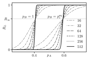
Figure 5: Numerical results for the dependence of $R_{L}$ as a function of $p_{A}$ for different values of $L$ for sublattice-selective percolation on the square lattice for $p_{B}=1$ (left curves) and $p_{B}=p_{c}^{\mathrm{sq}}$ (right curves). The horizontal line indicates the exact value of $R_{\infty}$ at $p_{c}^{\mathrm{sq}}$ from Ref. Newman and Ziff (2001).

In the infinite system limit, this quantity – denoted $R_{\infty}(p_{A})$ – exhibits a jump at the percolation threshold and we can obtain an estimate $p_{A,c}(L)$ of $p_{A,c}$ at the specified value of $p_{B}$ from the condition $R_{L}(p_{A,c}(L))=C$, where $C\in(0,1)$ is kept fixed upon varying $L$. The speed of convergence of $p_{A,c}(L)$ towards $p_{A,c}$ varies for different choices of $C$. For conventional site percolation Newman and Ziff Newman and Ziff (2001) suggest to take $C$ equal to the exactly known value of $R_{\infty}$ at $p_{c}^{\mathrm{sq}}$, which equals $0.6904...$, and find an algebraic asymptotic convergence,

$$p_{A,c}(L)-p_{A,c}\propto L^{-X},$$ (7)

conjecturing that $X=2+1/\nu$, which equals $2.75$ for $d=2$, leading thus to fast convergence. From our simulations, we observe no significant change in the threshold value of $R_{\infty}$ for the sublattice-selective case (cf., e.g., the crossing point values in Fig. 5). A formal prove of this statement would however still be valuable. In any case, we always fixed $C$ to the above value in order to fit $p_{A,c}(L)$ to the finite-size scaling in Eq. (7).

In particular, we performed finite-size calculations for system sizes between $L=16$ and $L=512$, doubling consecutive values of $L$. For each fixed value of $p_{B}$, we scaled the number of Monte Carlo steps (each corresponding to an initial configurations as in Fig. 3(a), followed by successively increasing $n_{A}$) with $L^{-3/2}$, taking $10^{7}$ steps at $L=16$. This procedure ensures a similar absolute statistical uncertainty on the estimator for $R_{L}(p_{A,c}(L))$ upon varying $L$, as it does for conventional percolation Newman and Ziff (2001): For a given probability $p_{A}$ the state function $R_{L}(p_{A})$ is either 1 or 0, so the uncertainty comes from the binomial distribution,

$$\sigma_{R_{L}}=\sqrt{\frac{R_{L}(p_{A})(1-R_{L}(p_{A}))}{M}},$$ (8)

where $M$ is the number of Monte Carlo steps. As the width of the critical region decreases as $L^{-1/\nu}$, the gradient $dR_{L}/dp_{A}$ of $R_{L}(p_{A})$ in the critical region increases as $L^{1/\nu}$. Together with Eq. (8), the uncertainty on $p_{A,c}$ thus scales as $\sigma_{p_{A,c}}\sim L^{-1/\nu}\sigma_{R_{L}}\sim L^{-1/\nu}M^{-1/2}$. To keep $\sigma_{p_{A,c}}$ constant, $M$ thus has to scale with $L^{-2/\nu}$. For $d=2$, the universal value is $\nu=4/3$, and this value will also be used for this uncertainty calculation here (this has no impact on the estimation of the critical exponents as performed in the next section – there will indeed also be no evidence that $\nu\neq 4/3$). Overall, the whole procedure was repeated one hundred times for a given $p_{B}$ in order to obtain the statistical error on all other estimated state functions. For the final transformation from $n_{A}$ to $p_{A}$, we used a narrow $p_{A}$-grid with a spacing of order $10^{-4}$.

Based on the numerical data, we obtain the values of $p_{A,c}$ for several values of $p_{B}$ reported in Tab. 1. Also included in this table are the values of the exponent $X$ that we obtain based on these fits (the values of $\chi^{2}/\mathrm{d.o.f.}$ are of $O(1)$). Overall, the estimated values of $X$ exhibit some scatter, but no significant systematic deviation from the proposed value for the conventional case Newman and Ziff (2001). The numerical results for $p_{A,c}$ that we obtain for the specific cases of $p_{B}=p_{c}^{\mathrm{sq}}$ and $p_{B}=1$ are in accord with the previously reported values, ensuring the overall accuracy of our approach.

$p_{B}$	$p_{A,c}$	$X$	$\nu$
$p_{c}^{\mathrm{sq}}$	$0.5927483(16)$	$2.80(10)$	$1.3318(4)$
$0.65$	$0.5431265(18)$	$2.66(13)$	$1.331(4)$
$0.7$	$0.5095937(13)$	$2.49(7)$	$1.3290(7)$
$0.75$	$0.4826738(13)$	$2.42(7)$	$1.3340(6)$
$0.8$	$0.46082758(35)$	$2.561(18)$	$1.3352(10)$
$0.85$	$0.4430110(13)$	$2.60(6)$	$1.3368(12)$
$0.9$	$0.4284801(17)$	$2.56(8)$	$1.33241(28)$
$0.95$	$0.4166941(8)$	$2.598(34)$	$1.3321(4)$
$1$	$0.4072524(6)$	$2.556(21)$	$1.3337(5)$

Table 1: Numerical results obtained for sublattice-selective percolation on the square lattice using the bipartite Newman–Ziff algorithm.

Based on the numerical values of $p_{A,c}$, and using the symmetry under the exchange of $p_{A}$ and $p_{B}$, we obtain the phase diagram for sublattice-selective percolation on the square lattice shown in Fig. 6.

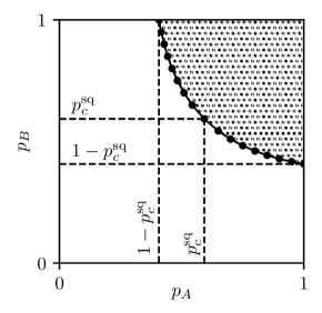
Figure 6: Phase diagram for sublattice-selective percolation on the square lattice, as obtained from the bipartite Newman–Ziff algorithm. The dotted regime is percolating.

III.2 Critical Exponents

In addition to the percolation threshold, we estimated the critical exponents for sublattice-selective percolation on the square lattice using appropriate finite-size scaling analysis Stauffer and Aharony (2018). We first consider the critical exponent $\nu$, which can be best estimated from the finite-size scaling of the gradient $R^{\prime}_{L}=dR_{L}/dp_{A}$ of $R_{L}(p_{A})$ near the percolation threshold,

$$R^{\prime}_{L}\propto L^{1/\nu},$$ (9)

We approximate $R^{\prime}_{L}$ from the slope of a linear regression within a $p_{A}$-range of $10^{-3}$ around the estimated value of $p_{A,c}$. The thus obtained estimates for $\nu$ are given in Tab. 1, and Fig. 7 shows bests fits to the numerical data for different values of $p_{B}$.

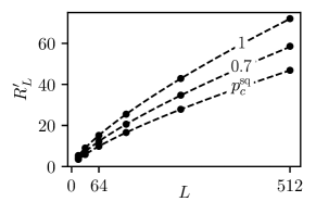
Figure 7: Fits of the numerical data for $R^{\prime}_{L}$ to the finite-size scaling form in Eq. (9) for different indicated values of $p_{B}$.

The values that we obtain for $\nu$ scatter with no systematic dependence of $p_{B}$, and taking their average gives $\nu=1.3352(11)$, which is in good agreement with $\nu=4/3$ for the $d=2$ universality class. We also find no indication that the critical exponents $\beta$ and $\gamma$ differ from their conventional values for $d=2$. In order to access these exponents, we consider the finite-size scaling forms

$$P_{L}=L^{-\beta/\nu}F_{P}[L^{1/\nu}(p_{A}-p_{A,c})]$$ (10)

for the estimate $P_{L}$ of the strength of the percolating cluster in terms of a scaling function $F_{P}$, and similarly

$$S_{L}=L^{\gamma/\nu}F_{S}[L^{1/\nu}(p_{A}-p_{A,c})]$$ (11)

for the mean number $S$ of finite clusters. From appropriate data-collapse plots, one can adjust the values of $\beta$ and $\gamma$, based on our previous estimates for $\nu$ and $p_{A,c}$, in order to obtain the best collapse within the critical region. Using such an analysis, we find that the best fit values are in fact in accord with the known values for conventional percolation in $d=2$. This is illustrated for several values of $p_{B}$ in Fig. 8. We thus conclude from our finite-size analysis, that the critical exponents for sublattice-selective percolation are in agreement with the universal values for $d=2$ percolation, supporting previous findings Scholl and Binder (1980); Idogaki and Uryû (1982).

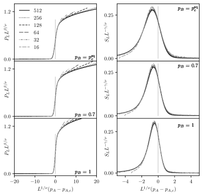
Figure 8: Data collapse plots for finite-size data labeled by $L$ for $P$ and $S$ for different values of $p_{B}$ using the critical exponents for $d=2$ percolation.

IV Lieb lattice

As a further example, we examine sublattice-selective percolation on the Lieb lattice, for which the case of uniform site percolation ($p_{A}=p_{B}$) has recently has been considered Oliveira et al. (2021). Since the Lieb lattice is in fact a decorated square lattice, sublattice-selective percolation is in this case equivalent to mixed bond-site percolation on the square lattice, with $p_{A}$ ($p_{B}$) specifying the bond (site) occupation probability. In particular, in the limit $p_{A}=1$ ($p_{B}=1)$, we obtain conventional pure site (bond) percolation on the square lattice, and thus $p_{B,c}=p_{c}^{\mathrm{sq}}$ ($p_{A,c}=1/2$) along these lines, respectively (here, we used the fact that the percolation threshold $1/2$ for bond percolation on the square lattice has been exactly determined Kesten (1980)). This shows explicitly that due to the inequivalence of the two sublattices of the Lieb lattice, the phase diagram is not symmetric in the $(p_{A},p_{B})$-plane. In Ref. Tarasevich and Van der Mark (1999), the general case of mixed bond-site percolation was considered for various lattices, including the square lattice. The phase diagram was numerically estimated, but only to comparably low accuracy, so that here we employed the bipartite Newman-Ziff algorithm in order to obtain more accurate values for the threshold line for sublattice-selective percolation on the Lieb lattice. The numerical results are provided in Tab. 2, and the corresponding phase diagram is shown in Fig. 9. Comparing the value of $p_{A,c}$ obtained for $p_{B}=1$ to the exact value ($1/2$) confirms the accuracy of our results. For estimating these numbers, $C$ was chosen identical to the square lattice value from the previous section, resulting in similarly fast convergence. Additionally, the previous estimate Oliveira et al. (2021) for the conventional ($p_{A}=p_{B}$) site percolation threshold $p_{c}^{\mathrm{Lieb}}$ on the Lieb lattice was improved using the Newman–Ziff algorithm. Along this line, we find that $C=0.68$ yields better convergence (however, even then the exponent $X\approx 1/\nu$ is significantly lower). The obtained value $p_{c}^{\mathrm{Lieb}}=0.7397120(17)$ is consistent with the previous best estimate Oliveira et al. (2021).

$p_{B}$	$p_{A,c}$
$0.6$	$0.983336(4)$
$0.65$	$0.8809405(10)$
$0.7$	$0.7965947(21)$
$0.75$	$0.7261839(20)$
$0.8$	$0.6666702(16)$
$0.85$	$0.6157944(18)$
$0.9$	$0.5718775(14)$
$0.95$	$0.5336113(21)$
$1$	$0.4999987(19)$

Table 2: Numerical results obtained for sublattice-selective percolation on the Lieb lattice using the bipartite Newman–Ziff algorithm.

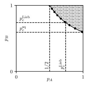
Figure 9: Phase diagram for sublattice-selective percolation on the Lieb lattice, as obtained from the bipartite Newman–Ziff algorithm. The dotted regime is percolating.

V Bethe lattice

To complement the above numerical study by exact analytical results, we finally consider sublattice-selective percolation on the Bethe lattice. We first consider the case $z=2$, essentially corresponding to the one-dimensional chain.

V.1 Percolation on a chain ($z=2$)

In this case, percolation occurs only at the singular point $(p_{A},p_{B})=(1,1)$. In order to extract the critical exponents upon approaching the percolation point along different lines within the $(p_{A},p_{B})$-plane, we next examine appropriate state functions.

A cluster containing $s$ occupied sites with one empty site to either side is called a $s$–cluster. The number of $s$–clusters per lattice site $n_{s}$ is a useful state function. Another way of looking at $n_{s}$ is that it is the probability of an arbitrary site to be the left-end site of an $s$–cluster. This is the case if the site to the left is empty, then $s$ consecutive sites are occupied, followed by another empty site. For $p_{A}=p_{B}=p$ the state function would be $n_{s}=(1-p)p^{2}(1-p)$, but for $p_{A}\neq p_{B}$ one has to consider whether the left end site is from the $A$ or $B$ sublattice, and whether $s$ is even or odd. The probability that an arbitrary site is from the $A$ or $B$ sublattice is equal to $1/2$, and from there on it is a matter of counting the $A$– and $B$–sublattice sites in the cluster to find

$$n_{s}(p_{A},p_{B})=\frac{1}{2}\left((\bar{p}_{B})^{2}p_{A}+(\bar{p}_{A})^{2}p_{B}\right)p_{A}^{(s-1)/2}p_{B}^{(s-1)/2}$$ (12)

for odd $s$, and

$$n_{s}(p_{A},p_{B})=\bar{p}_{A}\bar{p}_{B}p_{A}^{s/2}p_{B}^{s/2}$$ (13)

for even $s$, where $\bar{p}_{A}=1-p_{A}$, $\bar{p}_{B}=1-p_{B}$. The probability that an arbitrary site is part of a $s$–cluster is $n_{s}\cdot s$, so the probability that an arbitrary site is part of any cluster is given by

$$\sum_{s=1}^{\infty}n_{s}(p_{A},p_{B})s=\frac{1}{2}(p_{A}+p_{B}),$$ (14)

i.e., equivalent to the probability that an arbitrary site is occupied. From $n_{s}$, the mean cluster size $S$ can be evaluated, which equals the ratio of the second divided by the first moment of the cluster size distribution,

$$S(p_{A},p_{B}) =\frac{\sum_{s=1}^{\infty}n_{s}(p_{A},p_{B})s^{2}}{\sum_{s=1}^{\infty}n_{s}(p_{A},p_{B})s}$$

$$=\frac{p_{A}^{2}p_{B}+p_{A}p_{B}^{2}+4p_{A}p_{B}+p_{A}+p_{B}}{p_{A}+p_{B}-p_{A}^{2}p_{B}-p_{A}p_{B}^{2}},$$ (15)

which approaches 1 for $(p_{A},p_{B})\rightarrow(0,0)$ and diverges upon approaching $(1,1)$. We obtain the critical exponent $\gamma$ from analyzing the singular behaviour of $S$ near $(1,1)$. Fixing $p_{B}=1$, the asymptotic singularity is obtained as

$$S(p_{A},1) =\frac{p_{A}^{2}+6p_{A}+1}{1-p_{A}^{2}}$$

$$\sim 4(1-p_{A})^{-1},\quad\text{for $p_{A}\sim 1$},$$ (16)

so that $\gamma=1$. This asymptotic scaling also results upon approaching $(1,1)$ along any other line. Namely, for $p_{A}=1-r\cos(\phi),p_{B}=1-r\sin(\phi)$, with $\phi\in[0,\pi/2]$, the asymptotic behavior $S\sim 4/[(\cos(\phi)+\sin(\phi))\>r]$ for $r\rightarrow 0$ is obtained.

In order to obtain the correlation length $\xi$, we first calculate the correlation function (pair connectivity function) $g(r)$, i.e., the probability that an arbitrary occupied site is in the same cluster as another site a distance $r$ apart. Thus, there have to be $r-1$ consecutive occupied sites in between. For $p_{A}=p_{B}=p$ this is just $2p^{r}$ (2 for both directions), but for $p_{A}\neq p_{B}$ the parity of $r$ and the starting site have to be accounted for. The starting site is on the $A$ sublattice with probability $\frac{p_{A}}{p_{A}+p_{B}}$ and on the $B$ sublattice with probability $\frac{p_{B}}{p_{A}+p_{B}}$. Accounting for the parity of $r$ and the special case $r=0$, we obtain

$$g(r)=\begin{dcases}1,&r=0\\ \frac{4}{p_{A}+p_{B}}p_{A}^{(r+1)/2}p_{B}^{(r+1)/2},&\text{$r$ odd}\\ 2p_{A}^{r/2}p_{B}^{r/2},&\text{$r$ even}\end{dcases}.$$ (17)

The correlation length $\xi$ quantifies the length scale of the correlation function, and can also be viewed as the radius of the clusters that give the main contribution to the mean cluster size $S$ Stauffer and Aharony (2018). The formal definition is

$$\xi^{2}=\frac{\sum_{r}r^{2}g(r)}{\sum_{r}g(r)}.$$ (18)

A well-known identity in conventional percolation is that the sum over all $g(r)$ equals the mean cluster size, and this indeed also follows for sublattice-selective percolation, as we obtain

$$\sum_{r=0}^{\infty}g(r)=S.$$ (19)

The numerator in Eq. (18) can also be calculated and for $p_{B}=1$ scales as $(1-p_{A})^{-3}$ near the percolation threshold. Since $1/S$ scales as $(1-p_{A})$, the singularity of $\xi$ is thus obtained as

$$\xi^{2}(p_{A},1)=\frac{\sum_{r}r^{2}g(r)}{S}\sim(1-p_{A})^{-2},\quad\text{for $p_{A}\sim 1$},$$ (20)

and we extract the critical exponent $\nu=1$ for the divergence of $\xi$ near the percolation threshold.

The third state function that we consider is the strength of the percolating cluster $P$. For the chain this function is trivially 1 for $p_{A}=p_{B}=1$ and 0 otherwise. $P$ is thus constant with a discontinuity at the percolation threshold, and $\beta=0$.

In summary, for the one-dimensional case, the critical exponents for sublattice-selective percolation, specifying the behavior at the singular point $p_{A}=p_{B}=1$, are given by $\beta=0$, $\nu=1$, $\gamma=1$. These are the same exponents as for conventional percolation in $d=1$ Stauffer and Aharony (2018). Since only $p_{A}=p_{B}=1$ percolates, this conclusion may not be surprising.

V.2 Percolation threshold line for general $z$

The percolation condition on the Bethe lattice is that a chain of occupied sites reaches out to infinity. In other words, the system percolates if from some occupied site there exists a path of connected occupied sites that never ends (note that on the Bethe lattice such the path cannot form loops). If a chain of sites from a specific site up to some other site are occupied, at least one of the two neighbours going outwards also has to be occupied to have a percolating cluster. Hence, the mean number of occupied sites going outwards has to be at least one in order to form a percolating cluster. Furthermore, on the Bethe lattice the $A$ and $B$ sublattice alternate. The mean number of occupied sites going outwards can thus be calculated for $z$ neighbours by using two nested binomial distributions, one accounting for the mean number of $A$-sublattice sites and the other for the mean number of $B$-sublattice sites. This leads to the condition

$$1\overset{!}{=} \sum_{k=0}^{z-1}\binom{z-1}{k}p_{A}^{k}(1-p_{A})^{z-1-k}$$ (21)

$$\times\sum_{l=0}^{(z-1)k}l\binom{(z-1)k}{l}p_{B}^{l}(1-p_{B})^{(z-1)k-l},$$

which can be simplified to yield the condition for the percolation transition

$$p_{A}\>p_{B}=\frac{1}{(z-1)^{2}}.$$ (22)

Note that this result is also correct for $z=2$, treated in the previous section. The percolation threshold line for $z=3$ is at $p_{A}\>p_{B}=1/4$, which is plotted in Fig. 10. The larger $z$, the more area of the phase diagram is percolating, but here only $z=3$ will be further examined.

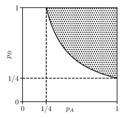
Figure 10: Phase diagram of sublattice-selective percolation on the Bethe lattice for $z=3$.

V.3 Scaling exponents for $z=3$

To access the critical exponents, three state functions will again be calculated: The strength of the percolating cluster $P$, the mean cluster size $S$, and the correlation length $\xi$. Here, we focus on $z=3$.

To obtain $P$, we first calculate the probability of a path not leading to infinity. Let $w_{A}$ ($w_{B}$) be the probability that an arbitrary $A$($B$) sublattice site does not lead to infinity, respectively. An $A$ sublattice site does not lead to infinity if the site itself is not occupied (given by the probability $1-p_{A}$) or if the two neighbours leading outwards do not lead to infinity (given by the probability $p_{A}w_{B}^{2}$), and similarly for a $B$ sublattice site. Altogether, this gives the recursive expressions

$$w_{A} =(1-p_{A})+p_{A}w_{B}^{2},$$ (23)

$$w_{B} =(1-p_{B})+p_{B}w_{A}^{2}.$$ (24)

This nonlinear system of equations has polynomials of degree four as solutions. The trivial solution is $w_{A}=w_{B}=1$, while the other real solution, denoted by $w^{P}_{A},w^{P}_{B}$ is rather lengthy, and given explicitly as a function of $p_{A}$ and $p_{B}$ in the appendix A. We note that for larger coordination number $z$, the corresponding recursion equations lead to higher-order equations for $w_{A}$ and $w_{B}$, for which closed expressions for the roots are known to not exist from Galois theory. For $p_{A}\>p_{B}<1/4$ there exists no infinite cluster and thus the trivial solution applies, while for $p_{A}\>p_{B}\geq 1/4$ the other real solution is valid, i.e.,

$$w_{A/B}=\begin{dcases}1,&4p_{A}\>p_{B}<1\\ w^{P}_{A/B}(p_{A},p_{B}),&4p_{A}\>p_{B}\geq 1\end{dcases}.$$ (25)

From these probabilities, the strength of the percolating cluster $P$ can be calculated as

$$P(p_{A},p_{B})=\frac{1}{2}\left(p_{A}(1-w_{B}^{3})+p_{B}(1-w_{A}^{3})\right),$$ (26)

since the probability that the center site is from the $A$ or $B$ sublattice is $1/2$ and the probability that the site is occupied and at least one neighbour leads to infinity equals $p_{A/B}(1-w_{B/A}^{3})$. The strength of the percolating cluster is plotted in Fig. 11.

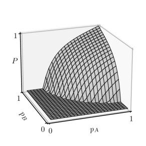
Figure 11: Strength $P$ of the percolating cluster for sublattice-selective percolation on the Bethe lattice for $z=3$.

In Fig. 12 cuts of $P$ at three different values of $p_{B}$ are shown, along with the function $6p_{A}p_{B}-3/2$, which yields the leading asymptotic of $P$ for conventional site-percolation on the Bethe lattice Stauffer and Aharony (2018). We thus find that near the percolation threshold line, i.e., for $p_{A}\gtrsim 1/(4p_{B}),p_{B}\geq 1/4$, the scaling behavior

$$P(p_{A},p_{B})\sim-3/2+6p_{A}p_{B}=-6p_{B}\left(\frac{1}{4p_{B}}-p_{A}\right),$$ (27)

emerges, implying a critical exponent $\beta=1$.

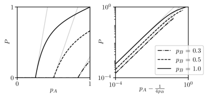
Figure 12: Strength $P$ of the percolating cluster as a function of $p_{A}$ for various values of $p_{B}$ (a) along with the function $6p_{A}p_{B}-3/2$ and (b) in shifted log-log form near the percolation threshold.

Next, the mean cluster size $S$ will be calculated. For this an arbitrary occupied starting site is considered and the mean mass of the cluster it belongs to is calculated. This approach is only valid below the percolation threshold line, i.e., for $4p_{A}p_{B}<1$, because otherwise the mass of the percolating cluster has to be accounted for as well. If the starting site belongs to the $A$($B$) sublattice, then let $S_{B}$ ($S_{A}$) be the contribution to the mean cluster size from each neighbour. The mean cluster size then is composed of the contribution from the center site plus the contribution from the three neighbours, so that

$$S(p_{A},p_{B})=1+3\frac{1}{p_{A}+p_{B}}(p_{A}S_{B}+p_{B}S_{A}).$$ (28)

The contributions $S_{A}$ and $S_{B}$ can be accessed recursively: If the starting site belongs to the $A$ sublattice, then a given neighbour only contributes a non–zero $S_{B}$ with probability $p_{B}$. The size of this contribution is the site itself plus $S_{A}$ for the two neighbours going outwards. With a similar reasoning for the $B$ sublattice, we thus obtain

$$\begin{rcases}S_{A}=p_{A}(1+2S_{B}),\\ S_{B}=p_{B}(1+2S_{A}),\end{rcases}\Rightarrow\quad\begin{array}[]{r@{\;}l}S_{A}=\frac{2p_{A}p_{B}+p_{B}}{1-4p_{B}p_{A}},\\ S_{B}=\frac{2p_{A}p_{B}+p_{A}}{1-4p_{B}p_{A}}.\end{array}$$ (29)

Both $S_{A}$ and $S_{B}$ diverge upon approaching the threshold condition $p_{A}p_{B}=\frac{1}{4}$. Hence, the behaviour of $S$ near the percolation threshold line can be described by

$$S(p_{A},p_{B})\sim\left(\frac{1}{4p_{B}}-p_{A}\right)^{-1},$$ (30)

giving the critical exponent $\gamma=1$.

Finally, the correlation length will be calculated. Here, the topological distance $r_{t}$ and Euclidean distance $r$ have to be distinguished. The topological distance between two sites, also called the chemical distance, is defined as the number of bonds that connect them, in contrast to the Euclidean distance, which is the distance that these points are apart in space. For $d=\infty$, the conversion becomes easy because all bonds are pair–wise perpendicular, so that the Euclidean distance can be calculated by the generalized Pythagorean theorem as $r=\sqrt{r_{t}}$  Peruggi et al. (1984).

The correlation function $g(r)=g(\sqrt{r_{t}})$, for $4p_{A}p_{B}<1$, gives the mean number of sites connected to a given occupied site at a topological distance $r_{t}$, corresponding to the Euclidean distance $r$. At $r_{t}=0$ the center site is already occupied, while at $r_{t}=1$ the site has 3 neighbours and from there on the number of neighbours doubles in each step, and the probabilities are otherwise the same as for the case of the chain, so that we obtain

$$g(\sqrt{r_{t}})=\begin{dcases}1,&r_{t}=0\\ 3\cdot 2^{r_{t}-1}\frac{2}{p_{A}+p_{B}}p_{A}^{\frac{(r_{t}+1)}{2}}p_{B}^{\frac{(r_{t}+1)}{2}},&\text{$r_{t}$ odd}\\ 3\cdot 2^{r_{t}-1}p_{A}^{r_{t}/2}p_{B}^{r_{t}/2},&\text{$r_{t}$ even}\end{dcases}$$

The Euclidean correlation length can also be expressed in terms of the topological distance, since

$$\xi^{2}=\frac{\sum_{r\in\{0,1,\sqrt{2},\sqrt{3},...\}}r^{2}g(r)}{\sum_{r\in\{0,1,\sqrt{2},\sqrt{3},...\}}g(r)}=\frac{\sum_{r_{t}\in\mathbb{N}_{0}}r_{t}g(\sqrt{r_{t}})}{\sum_{r_{t}\in\mathbb{N}_{0}}g(\sqrt{r_{t}})}.$$ (31)

We note that the identity $\sum_{r}g(r)=S$ is again satisfied, and hence the denominator of Eq. (31) behaves like $(1-4p_{A}p_{B})^{-1}$ for $p_{A}\sim 1/{p_{B}}$. Furthermore, we find that the numerator behaves like $(1-4p_{A}p_{B})^{-2}$ for $p_{A}\sim{1}/{p_{B}}$, and together the singularity of $\xi$ near the percolation threshold is given by

$$\xi(p_{A},p_{B})\sim\left(\frac{1}{4p_{B}}-p_{A}\right)^{-\frac{1}{2}},$$ (32)

so that $\nu=1/2$. We thus obtain the same critical exponents as for conventional percolation on the Bethe lattice.

VI Conclusions

We presented an adapted Newman–Ziff algorithm to sublattice-selective percolation on bipartite lattices and applied it to accurately determine the percolation threshold lines for the square lattice and the planar Lieb lattice. The latter case relates to mixed bond-site percolation on the square lattice and our numerical results for the percolation threshold line refine previous estimates. Our numerical estimates for the critical exponents at the percolation transition are consistent with the universality class for percolation in $d=2$.

In addition, we examined sublattice-selective percolation on the Bethe lattice, which was in fact the geometry considered in the pioneering work on percolation by Flory in the context of polymerization Flory (1941). For this case, we obtained the exact percolation threshold line and critical exponents for $z=2$ and $z=3$, which are again in accord with the values for conventional percolation. Given that the sites of the square lattice have a uniform coordination number of $z=4$, it may be interesting to compare its phase diagram to the one of the Bethe lattice with $z=4$. Such a comparison is shown in Fig. 13, illustrating the substantially larger percolating regime for the latter case. Indeed, the absence of closed loops for a chain of connected sites leads to an overall prior appearance of the percolating cluster upon increasing the site occupation probabilities on the Bethe lattice. We checked explicitly, that a rescaling of the analytic expression for the percolation threshold line for the $z=4$ Bethe lattice to match the ends points at $p_{A}=1$ and $p_{B}=1$ does not fit the full numerical data.

Related to the last point, we note that the authors of Ref. Tarasevich and Van der Mark (1999) considered various proposed analytic expressions for the general functional form of the percolation threshold line for mixed bond-site percolation. They observed clear systematic deviations from the numerical data for low-coordinated lattices. Based on our refined data on the Lieb lattice, we can also exclude the general validity of these expressions for the square lattice. It thus remains an interesting open question for further research to derive analytical expressions for the percolation threshold line for sublattice-selective as well as mixed bond-site percolation, respectively. We hope that our refined numerical data will be valuable as a benchmark for such investigations.

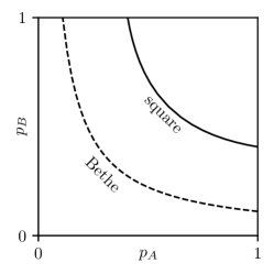
Figure 13: Comparison between the percolation threshold line for sublattice-selective percolation on the square lattice (solid line) and the Bethe lattice with $z=4$ (dashed line).

Appendix A Non-trivial real solution for the $z=3$ Bethe lattice

The non-trivial real solution to Eqs. (23) and (24), obtained using the Sympy Python library, is

$$w^{P}_{A/B}= -\frac{1}{3}\left(\frac{1-a_{A/B}}{c_{A/B}}+c_{A/B}+1\right),\quad\mathrm{where}$$

$$a_{A/B}= \frac{3\left(2-p_{B/A}\right)}{p_{B/A}},$$

$$b_{A/B}= \frac{27\left(-p_{A/B}p_{B/A}^{2}+2p_{A/B}p_{B/A}-1\right)}{p_{A/B}p_{B/A}^{2}},$$

$$c_{A/B}= \sqrt[3]{\frac{\sqrt{-4\left(1-a_{A/B}\right)^{3}+\left(2-3a_{A/B}+b_{A/B}\right)^{2}}}{2}+1-\frac{3}{2}a_{A/B}+b_{A/B}}.$$

References

- Flory (1941) P. J. Flory, Journal of the American Chemical Society 63 (1941).
- Stauffer and Aharony (2018) D. Stauffer and A. Aharony, Introduction To Percolation Theory (Taylor & Francis, 2018).
- Lee (2008) M. J. Lee, Physical Review E - Statistical, Nonlinear, and Soft Matter Physics 78 (2008), 10.1103/PhysRevE.78.031131.
- Jacobsen (2015) J. L. Jacobsen, Journal of Physics A: Mathematical and Theoretical 48, 454003 (2015).
- Smirnov and Werner (2001) S. Smirnov and W. Werner, Mathematical Research Letters 8, 729 (2001).
- Scholl and Binder (1980) F. Scholl and K. Binder, Zeitschrift für Physik B Condensed Matter 39 (1980).
- Sykes and Essam (1964) M. F. Sykes and J. W. Essam, Journal of Mathematical Physics 5 (1964).
- Idogaki and Uryû (1982) T. Idogaki and N. Uryû, Physics Letters A 90, 367 (1982).
- Idogaki and Uryu (1982) T. Idogaki and N. Uryu, Journal of Physics C: Solid State Physics 15, L1077 (1982).
- Idogaki and Uryû (1983) T. Idogaki and N. Uryû, Journal of Magnetism and Magnetic Materials 31-34, 1257 (1983).
- Idogaki et al. (1995) T. Idogaki, M. Hitaka, and K. Masuda, Journal of Magnetism and Magnetic Materials 140-144, 1517 (1995).
- Ueda et al. (2000) H. Ueda, A. Tanaka, T. Iwashita, and T. Idogaki, Physica B: Condensed Matter 284-288, 1201 (2000).
- Newman and Ziff (2000) M. E. J. Newman and R. M. Ziff, Phys. Rev. Lett. 85, 4104 (2000).
- Newman and Ziff (2001) M. E. J. Newman and R. M. Ziff, Phys. Rev. E 64, 016706 (2001).
- Oliveira et al. (2021) W. S. Oliveira, J. P. de Lima, N. C. Costa, and R. R. dos Santos, Phys. Rev. E 104, 064122 (2021).
- Hoshen and Kopelman (1976) J. Hoshen and R. Kopelman, Phys. Rev. B 14 (1976).
- Kesten (1980) H. Kesten, Communications in Mathematical Physics 74, 41 (1980).
- Tarasevich and Van der Mark (1999) Y. Y. Tarasevich and S. C. Van der Mark, International Journal of Modern Physics C 10, 1193 (1999).
- Peruggi et al. (1984) F. Peruggi, F. di Liberto, and G. Monroy, Physica A: Statistical Mechanics and its Applications 123 (1984), 10.1016/0378-4371(84)90110-9.