$b$-Hurwitz numbers from Whittaker vectors for $\mathcal{W}$-algebras

Abstract.

We show that $b$-Hurwitz numbers with a rational weight are obtained by taking an explicit limit of a Whittaker vector for the $\mathcal{W}$-algebra of type $A$. Our result is a vast generalization of several previous results that treated the monotone case, and the cases of quadratic and cubic polynomial weights. It also provides an interpretation of the associated Whittaker vector in terms of generalized branched coverings that might be of independent interest. Our result is new even in the special case $b=0$ that corresponds to classical hypergeometric Hurwitz numbers, and implies that they are governed by the topological recursion of Eynard–Orantin. This gives an independent proof of the recent result of Bychkov–Dunin-Barkowski–Kazarian–Shadrin.

1. Introduction

Hurwitz theory, in its simplest form, counts branched coverings of algebraic curves. First considered in 1891 by Hurwitz [Hur91] who showed that Hurwitz numbers can be expressed in terms of counting permutation factorizations, Hurwitz theory has recently been found to have fascinating connections to integrable hierarchies, Gromov–-Witten theory, and topological recursion ([Pan00, ELSV01, OP06, GJ08, Eyn14] to mention a few). In the last two decades, various generalizations of simple Hurwitz numbers have been studied in many different contexts.

The most notable cases include Grothendieck dessins d’enfants and more generally constellations [BMS00], monotone Hurwitz numbers [GGPN14], orbifold Hurwitz numbers [JPT11], and monotone orbifold Hurwitz numbers [KLS19] among others. An approach unifying all these different classes was introduced in [GPH17] which defined $G$-weighted Hurwitz numbers $H^{(0)}_{G;g}(\mu_{1},\dots,\mu_{n})$, where the weight $G(z):=\sum_{i\geq 0}g_{i}z^{i}$ is a formal power series. The generating function of weighted Hurwitz numbers is a tau-function of hypergeometric type of the KP, or more generally the 2-Toda integrable hierarchies [OS00], and is given by the following explicit formula:

(1) $$\tau_{G}^{(0)}:=\sum_{\begin{subarray}{c}n\geq 0,\\ \lambda\vdash n\end{subarray}}\check{s}_{\lambda}(\mathbf{p})\prod_{\square\in\lambda}\frac{G(\hbar\cdot c(\square))}{\hbar}=\exp\left(\sum_{\begin{subarray}{c}g\in\mathbb{Z}_{\geq 0},\\ n\in\mathbb{Z}_{\geq 1}\end{subarray}}\hbar^{2g-2+n}\sum_{\mu\colon\ell(\mu)=n}H^{(0)}_{G;g}(\mu_{1},\dots,\mu_{n})\cdot p_{\mu}\right),$$

where $\check{s}_{\lambda}(\mathbf{p})$ is an appropriately normalized Schur function expressed in the basis of power-sum symmetric functions $\mathbf{p}=(p_{k})_{k\geq 1}$, and $c(\square):=x-y$ is the content of the box $\square=(x,y)$.

1.1. $b$-deformed weighted Hurwitz numbers

For many classical examples of Hurwitz numbers (i.e., for specific choices of the weight $G$), the generating function $\tau^{(0)}_{G}$ can be realized as the partition function of a matrix model. Such matrix models admit a natural one-parameter deformation, which first arose in the context of log-gases with the inverse temperature $\beta$, and it is well-understood that its partition function admits an expansion in terms of Jack polynomials $J_{\lambda}^{(\alpha)}(\mathbf{p})$ with the parameter $\alpha=\frac{2}{\beta}$ [For10, BH03, BEMPF12]. Motivated by these results and the universality of weighted Hurwitz numbers, Chapuy and the second author defined in [CD22] $G$-weighted $b$-Hurwitz numbers $H^{(b)}_{G;g}(\mu_{1},\dots,\mu_{\ell})$, a one-parameter deformation of classical weighted Hurwitz numbers, satisfying an analogous relation to (1):

$$\tau_{G}^{(b)}:=\sum_{\begin{subarray}{c}n\geq 0,\\ \lambda\vdash n\end{subarray}}\check{J}_{\lambda}^{(1+b)}(\mathbf{p})\prod_{\square\in\lambda}\frac{G(\hbar\cdot c_{1+b}(\square))}{\hbar}=\exp\left(\sum_{\begin{subarray}{c}g\in\frac{1}{2}\mathbb{Z}_{\geq 0},\\ n\in\mathbb{Z}_{\geq 1}\end{subarray}}\frac{\hbar^{2g-2+n}}{1+b}\sum_{\mu\colon\ell(\mu)=n}H^{(b)}_{G;g}(\mu_{1},\dots,\mu_{n})\cdot p_{\mu}\right),$$

where $c_{1+b}(x,y):=(b+1)\cdot x-y-b$ is the $b$-deformation of the content, and $\check{J}^{(1+b)}_{\lambda}(\mathbf{p})$ is an appropriately normalized Jack polynomial with the condition $\check{J}_{\lambda}^{(1)}(\mathbf{p})=\check{s}_{\lambda}(\mathbf{p})$ so that the $H^{(b)}_{G;g}$ agree with the $H^{(0)}_{G;g}$ of (1) when $b=0$ (see LABEL:{sub:Jack} for more details).

The reparametrization $\alpha=1+b$ comes from a fascinating enumerative property which was conjectured in several special cases covered by weighted $b$-Hurwitz numbers – for any $\mu_{1},\dots,\mu_{n}$ the quantity $|\mu|\cdot H^{(b)}_{G;g}(\mu_{1},\dots,\mu_{n})\in\mathbb{Z}_{\geq 0}[b][g_{0},g_{1},\dots]$ is a polynomial in $b$ with non-negative integer coefficients. This conjecture was proved in full generality by Chapuy and the second author in [CD22]. They interpreted weighted $b$-Hurwitz numbers as an explicit one-parameter interpolation between classical (complex) Hurwitz theory and its non-orientable (real) version. Additionally, in the case of a rational weight $G(z)$, which is the topic of our article, Ruzza recently found in [Ruz23] an elegant combinatorial interpretation of $H^{(b)}_{G;g}(\mu_{1},\dots,\mu_{n})$ in terms of colored $b$-monotone Hurwitz maps introduced in [BCD23].

Weighted $b$-Hurwitz numbers have already been proved to encompass many models from mathematical physics, enumerative geometry, and combinatorics: specific polynomial weights cover the case of Gaussian $\beta$-ensembles [BCD23], the monotone case was shown in [BCD23] to cover the $\beta$-deformation of the Harish-Chandra/Itzykson–Zuber (HCIZ) integral introduced by Herz in [Her55] as a multivariate Bessel function and reintroduced in the physics literature in [BH03] (see also [BEMPF12]) and the $\beta$-deformation of the Brézin–Gross–Witten integral introduced in [MMS11]. The case of Jacobi $\beta$-ensembles and Laguerre $\beta$-ensembles are also covered by rationally-weighted $b$-Hurwitz numbers as recently shown in [Ruz23]. The very special case $b=1$ of simple Hurwitz numbers was rediscovered in [BF21, HM22] in the context of surgery theory, tropical geometry and combinatorics (see [BD22] for different and more general combinatorial models).

1.2. Cut-and-join equation and $\mathcal{W}$-constraints

Some of the main tools in understanding the structure of classical Hurwitz numbers are cut-and-join equations that determine $H^{(0)}_{G;g}$ uniquely. These equations can be obtained by interpreting Hurwitz numbers as factorizations of a permutation into transpositions, and by analyzing the effect of multiplying a permutation by a transposition, which either cuts a cycle into two new cycles, or joins two cycles into a new cycle. In classical examples where the weight $G(z)$ is relatively simple, one can understand these equations in terms of the Jucys–Murphy elements that further lead to methods employing the representation theory of the symmetric group and so-called semi-infinite wedge representations (see for instance [BDK⁺23] and references therein). Cut-and-join equations turned out to be crucial in proving various structural properties of Hurwitz numbers. They were used to prove the Eynard–Orantin topological recursion (discussed in more detail in Section 1.3) for the classical [BMn08, EMS11], the monotone [GGPN14, DDM17a] and other models of Hurwitz numbers, polynomiality and ELSV-type formulas [GJV05, BDK⁺23].

On the other hand, finding cut-and-join equations for the arbitrary $b$ requires new ideas due to the lack of an analogous combinatorial/representation theoretic interpretation. An approach based on the theory of Jack polynomials was proposed by Chapuy and the second author in [CD22], where they found a Lax structure that allowed them to obtain certain cut-and-join-type equations for $\tau_{G}^{(b)}$. These equations are of infinite degree unless $G(z)$ is a polynomial, which makes it difficult to extract some interesting information from them (extracing constraints that refine the cut-and-join-type equation is highly non-trivial even in the polynomial case, see [BN23] for the case of cubic polynomial weight).

However, in the special case of monotone $b$-Hurwitz numbers, [BCD23] found a different cut-and-join equation and used it to produce Virasoro constraints (also obtained by [Yan11] prior to discovering the enumerative interpretation of $\tau_{G}^{(b)}$). One of the key contributions of our paper is the proof of a cut-and-join-type equation of finite degree for arbitrary rational weights, extending the monotone case. More importantly, we find that the underlying structure of this cut-and-join equation is closely related to the structure of a vertex algebra known as the $\mathcal{W}$-algebra (a generalization of the Virasoro algebra). An important insight is to use lattice paths as a combinatorial tool that simultaneously encodes certain operators acting on $\tau^{(b)}_{G}$ as well as the $\mathcal{W}$-algebra structure. As a consequence we show that $\tau^{(b)}_{G}$ for any rational weight $G(z)$ can be obtained from a Whittaker vector for a $\mathcal{W}$-algebra of type $A$ via some simple substitutions and limits.

More concretely, we work with the algebra $\mathcal{W}^{\mathsf{k}}(\mathfrak{gl}_{r})$ (where the level $\mathsf{k}$ is related to $b$), and a specific representation of it, defined using (20). Then, we use Airy structure techniques (introduced in [KS18, BBC⁺18, BBCC21]) to construct a Whittaker vector $\mathcal{Z}$ for $\mathcal{W}^{\mathsf{k}}(\mathfrak{gl}_{r})$ satisfying the following constraints

$$\mathsf{W}^{i}_{k}\mathcal{Z}=\Omega_{i}\delta_{k,0}\mathcal{Z}\,\qquad\forall i\in[r],k\in\mathbb{Z}_{\geq 0},$$

where $\big{(}\mathsf{W}^{i}_{k}\big{)}_{k\in\mathbb{Z},i\in[r]}$ are the modes of a set of strong generators for $\mathcal{W}^{\mathsf{k}}(\mathfrak{gl}_{r})$, and $\Omega_{i}$ is a certain function of the parameters appearing in the rational weight $G(z)$. Note that the vector $\mathcal{Z}$ is not the highest weight vector of the representation we are working in, but rather a Whittaker vector (see Remark 4.1 for more details). An abbreviated version of one of our main results Theorem 4.8 is as follows.

Theorem 1.1.

Consider the generating function $\tau^{(b)}_{G}$ of weighted $b$-Hurwitz numbers for an arbitrary rational weight, say $G(z)=\frac{\prod_{i=1}^{p}(P_{i}+z)}{\prod_{i=1}^{q}(Q_{i}-z)}$ for some $p,q\geq 0$. The function $\tau^{(b)}_{G}$ is an (explicit) limit of the Whittaker vector $\mathcal{Z}$ for $\mathcal{W}^{\mathsf{k}}(\mathfrak{gl}_{r})$ where $r=\max(p,q+2)$.

A slight variant of Theorem 1.1 states that the Gaiotto vector from the celebrated AGT conjecture [AGT10, SV13, MO19, BBCC21] is closely related to the generating function of certain weighted $b$-Hurwitz numbers, which might shed new light on the relation between Toda conformal blocks and the Nekrasov instanton partition function (see Remark 4.9 for more details).

1.3. Topological recursion

In various contexts [BBC⁺18, BBCC21], it has been proved using the formalism of Airy structures that $\mathcal{W}$-constraints are closely related to the topological recursion (TR) formalism, originally invented by Eynard–Orantin [EO07]. TR is a universal procedure which produces certain enumerative invariants $\omega_{g,n}$, called correlators for a fixed topology of genus $g$ with $n$ boundaries. These correlators are built recursively from the initial data of a spectral curve $(\Sigma,x,y,\omega_{0,2})$, consisting of a Riemann surface $\Sigma$, two non-constant meromorphic functions $x,y$ on $\Sigma$, and a choice of a canonical symmetric bi-differential $\omega_{0,2}$ on $\Sigma\times\Sigma$.

[BCU] proves that the Whittaker vector $\mathcal{Z}$ at the self-dual level $\mathsf{k}=1-r$, which corresponds to choosing $b=0$, can be computed using topological recursion on a certain spectral curve. Combining this with Theorem 1.1, and taking appropriate limits allow us to deduce that the classical rationally weighted Hurwitz numbers can be computed by TR, which was first proved in [BDBKS20]. This is one of the most important structural results in Hurwitz theory, and we provide a new and independent proof of it in Section 5 from the $\mathcal{W}$-algebra perspective:

Theorem 1.2.

Consider the rational weight $G(z)=\frac{\prod_{i=1}^{p}(P_{i}+z)}{\prod_{i=1}^{q}(Q_{i}-z)}$ for some $p,q\geq 0$. Let $\omega_{g,n}$ denote the correlators obtained from TR on the spectral curve $\left({\mathbb{C}\mathbb{P}}^{1},x,\omega_{0,1}=ydx,\omega_{0,2}\right)$, with

$$x(z)=\frac{z}{G(z)},\quad y(z)=G(z),\quad\omega_{0,2}(z_{1},z_{2})=\frac{\mathsf{d}z_{1}\mathsf{d}z_{2}}{(z_{1}-z_{2})^{2}}.$$

Then, expanding the correlators $\omega_{g,n}(z_{1},\ldots,z_{n})$ near $z_{1},\dots,z_{n}=0$ gives $G$-weighted Hurwitz numbers:

$$\omega_{g,n}(z_{1},\dots,z_{n})=\sum_{\mu_{1},\dots,\mu_{n}\in\mathbb{Z}_{\geq 1}}H^{(0)}_{G;g}(\mu_{1},\dots,\mu_{n})|\operatorname{Aut}(\mu)|\prod_{i=1}^{n}\mu_{i}x_{i}(z)^{\mu_{i}-1}\mathsf{d}x(z_{i})\,.$$

Let us comment briefly on the history of this theorem. Before the breakthrough of [ACEH20] where Hurwitz numbers weighted by arbitrary polynomials $G$ was proved to be governed by TR, each model of interest was treated case by case over a decade: [BMn08, EMS11] (simple Hurwitz numbers), [DDM17b] (monotone), [KPS22] (monotone orbifold) to name just a few. Finally, [BDBKS20] gave a uniform proof of a more general result, that in particular, covers the case of arbitrary rational weights $G$ Theorem 1.2 (see also [BCCGF22, BDBKS22] for the most recent developments concerning double Hurwitz numbers that we do not consider in this paper).

The existing proofs of Theorem 1.2 rely heavily on the KP integrability of the generating function $\tau^{(0)}_{G}$ that is specific to the $b=0$ case and does not have even a conjectural extension to arbitrary $b$. In our proof, we use the underlying $\mathcal{W}$-algebra structure controlling Hurwitz theory for arbitrary $b$ as we prove in Theorem 1.1, and the close relationship between $\mathcal{W}$-algebras and the Eynard–Orantin topological recursion. In fact, this leads to the following natural question:

What is the correct generalization (if any) of the Eynard–Orantin topological recursion that will govern enumerative properties of weighted $b$-Hurwitz numbers?

While the $\mathcal{W}$-constraints of (1.2) hold for any $b$, the analytic side that mimics the original construction of Eynard–Orantin is still under investigation. There are two differing approaches to extend the Eynard–Orantin topological recursion to arbitrary $b$. One approach, which has been developed in [CEM11, BE19, BBCC21] is to replace the initial data of a spectral curve by a non-commutative spectral curve (essentially, a $D$-module on the spectral curve) and goes by the name of non-commutative topological recursion. The underlying $\mathcal{W}$-algebra structure of this non-commutative topological recursion was explored thoroughly in [BBCC21] for a specific example, which, in Hurwitz theory corresponds to the case where $1/G(z)$ is a polynomial (see Remark 4.9). While it seems difficult to extract analytic properties of $b$-Hurwitz numbers directly from non-commutative TR, this connection is an interesting problem that deserves further study.

Another promising approach is the so-called refined topological recursion. A refinement was first attempted by Chekhov and Eynard [CE06] in the case of $\beta$-deformed matrix models, and its mathematical formulation for degree-$2$ curves was recently carried out by Kidwai and the third author in [KO23, Osu23]. The initial data is upgraded to a refined spectral curve which comes with a new differential $\omega_{\frac{1}{2},1}$. In subsequent work we will show that our main result Theorem 1.1 implies that the refined TR computes the tau function of some classes of weighted $b$-Hurwitz numbers. This will explain a mysterious structural difference between rational parameterizations of generating series of orientable and non-orientable combinatorial maps (see [DL22] and references therein).

All in all, our main theorems give the first answer to the natural question of relating weighted $b$-Hurwitz numbers with TR, and form the foundation for further investigation into this topic.

1.4. Notation

Given an integer $n\geq 1$, we will denote the set $\{1,\dots,n\}$ by $[n]$, and given integers $2\leq m\leq n$, we define the set $[m..n]:=[n]\setminus[m-1]$ ($[0]:=\emptyset$ by convention). We denote by $\mathcal{F}_{<}(A,B)$ a set of strictly increasing functions $f\colon A\rightarrow B$, i.e.  $f(a)<f(a^{\prime})$ for all $a<a^{\prime}$. We use a bold face to indicate that we are working with a family of indeterminates indexed by positive integers, e.g.  $\mathbf{p}=(p_{1},p_{2},\dots),\mathbf{g}=(g_{1},g_{2},\dots),\mathbf{x}=(x_{1},x_{2},\dots)$, etc. For a ring $R$ we denote by $R[\mathbf{x}]$, $R(\mathbf{x})$, $R\llbracket\mathbf{x}\rrbracket$, and $R(\!(\mathbf{x})\!)$ the polynomial, rational, formal power series, and formal Laurent series, respectively, rings over $R$. For a function $F$ of the variables $\mathbf{p}$, we use the notation $[p_{i_{1}}\cdots p_{i_{n}}]F$ to denote the coefficient of the monomial $p_{i_{1}}\cdots p_{i_{n}}$ in $F$.

In this paper we work with a non-trivial reparametrization of $\tau_{G}^{(b)}$, which reveals more remarkable properties of $b$-Hurwitz numbers. We will denote the reparametrized function by $\tau_{G}^{(\mathfrak{b})}$, where the main parameter is $\mathfrak{b}=\sqrt{\alpha}^{-1}-\sqrt{\alpha}$ (see (10)). We summarize the relation between the four equivalent parameters $\alpha,b,\mathsf{k},\mathfrak{b}$ that will appear in our paper:

(2) $$\mathfrak{b}=\sqrt{\alpha}^{-1}-\sqrt{\alpha}=-\frac{b}{\sqrt{1+b}}=\mathsf{k}+r-1.$$

Acknowledgements

NKC acknowledges the support of the ERC Starting Grant 948885, and the Royal Society University Research Fellowship. MD is supported by Narodowe Centrum Nauki, grant 2021/42/E/ST1/00162. KO is supported by JSPS KAKENHI Grant number 22KJ0715 and 23K12968. We would like to thank the organizers of the program "TR SALENTO 2022", where our collaboration on this project begun. We would also like to thank Gaëtan Borot and Thomas Creutzig for helpful discussions.

2. Cut-and-join equation for weighted $b$-Hurwitz numbers

In this section, we will derive a specific cut-and-join equation for weighted $b$-Hurwitz numbers, which will turn out to be related to $\mathcal{W}$-algebra representations in the later sections.

2.1. Jack polynomials

We call $\lambda$ an integer partition of $n$ if $\lambda$ is a finite sequence $\lambda_{1}\geq\cdots\geq\lambda_{\ell}>0$ of nonnegative integers that sums up to $n=:|\lambda|$. We denote it by $\lambda\vdash n$, and its number of parts $\ell$ is denoted $\ell(\lambda)$. Sometimes we use the notation $\lambda=(1^{m_{1}(\lambda)},2^{m_{2}(\lambda)},\dots)$, where $m_{i}(\lambda)$ denotes the number of parts of $\lambda$ that are equal to $i$. The set of partitions of the same size is linearly ordered:

$$\lambda\leq\mu\iff\sum_{i=1}^{j}\lambda_{i}\leq\sum_{i=1}^{j}\mu_{i}\qquad\forall j.$$

We will interchangeably use the terms an integer partition $\lambda$ and a Young diagram $\lambda$ and we associate the latter with the collection of boxes $\{\lambda\ni\square:=(x,y)\colon 1\leq y\leq\ell(\lambda),1\leq x\leq\lambda_{y}\}$. For such a box $\square=(x,y)\in\lambda$ we define its $\alpha$-deformed content as the quantity $c_{\alpha}(x,y):=\alpha(x-1)-(y-1)$. This quantity plays an important role in theory of Jack polynomials, that we will briefly describe following [Sta89, Mac95].

Let $R$ be a ring and let $R(\alpha)[\mathbf{p}]$ denote the polynomial ring in infinitely many variables $\mathbf{p}=(p_{k})_{k\geq 1}$ over the ring $R(\alpha)$. The following operator, called the Laplace–Beltrami operator, acts on $R(\alpha)[\mathbf{p}]$:

$$D_{\alpha}:=\frac{1}{2}\left(\sum_{k,\ell\geq 1}\alpha k\ell\cdot p_{k+\ell}\partial_{p_{k}}\partial_{p_{\ell}}+\sum_{k,\ell\geq 1}\alpha(k+\ell)\cdot p_{k}p_{\ell}\partial_{p_{k+\ell}}+(\alpha-1)\sum_{k\geq 1}k(k-1)p_{k}\partial_{p_{k}}\right).$$

Jack polynomials $J^{(\alpha)}_{\lambda}$ are elements of $\mathbb{Q}(\alpha)[\mathbf{p}]$ that are indexed by integer partitions $\lambda$. Consider the following grading on the ring $\mathbb{Q}(\alpha)[\mathbf{p}]$ defined on the basis: $\deg(\alpha):=0,\deg(p_{k}):=k$. Then, the Jack polynomial $J^{(\alpha)}_{\lambda}$ can be characterized (up to a normalization factor) as the unique homogeneous polynomial of degree $|\lambda|$ such that:

1. it is an eigenfunction of the Laplace–Beltrami operator: $D_{\alpha}J^{(\alpha)}_{\lambda}=\sum_{\square\in\lambda}c_{\alpha}(\square)J^{(\alpha)}_{\lambda},$

2. the transition matrix from $\{J^{{(\alpha)}}_{\lambda}\}_{|\lambda|=n}$ to the monomial symmetric functions $\{m_{\lambda}(\mathbf{x})\}_{|\lambda|=n}$ is lower triangular after identifying $p_{k}$ with the power-sum symmetric functions $p_{k}=p_{k}(\mathbf{x}):=\sum_{i}x_{i}^{k}$.

We will work with the integral Jack polynomials which are normalized such that the coefficient $[p_{1}^{|\lambda|}]J^{(\alpha)}_{\lambda}=1$. The quantity

$$j^{(\alpha)}_{\lambda}:=\prod_{\square\in\lambda}\operatorname{hook}_{\lambda}(\square)\cdot\operatorname{hook}_{\lambda}(\square)^{\prime},$$

with

$$\operatorname{hook}_{\lambda}(\square):=\alpha(\lambda_{y}-x)+\lambda_{x}^{\prime}-y+1,\quad\operatorname{hook}_{\lambda}(\square)^{\prime}=\alpha(\lambda_{y}-x+1)+(\lambda_{x}^{\prime}-y)$$

is the normalization factor. One can define a scalar product on $\mathbb{Q}(\alpha)[\mathbf{p}]$ for which the $J_{\lambda}^{(\alpha)}$ give an orthogonal basis with the norm $\|J_{\lambda}^{(\alpha)}\|^{2}=j_{\lambda}^{(\alpha)}$. One can show that this is precisely the $\alpha$-deformed Hall scalar product for which $p_{\lambda}:=\prod_{i=1}^{\ell(\lambda)}p_{\lambda_{i}}$ is orthogonal with the classical norm:

$$\langle p_{\lambda},p_{\lambda}\rangle=\alpha^{\ell(\lambda)}\frac{\prod_{i\geq 1}m_{i}(\lambda)!i^{m_{i}(\lambda)}}{|\lambda|!}.$$

Let us define the operators $(\mathsf{J}^{1}_{k})_{k\in\mathbb{Z}}$ acting on $R[\tilde{\mathbf{p}}]\llbracket\hbar\rrbracket$ by

(3) $$\mathsf{J}^{1}_{k}=\begin{cases}\hbar k\cdot\partial_{\tilde{p}_{k}}&\text{ if }k>0,\\ 0&\text{ if }k=0,\\ \hbar\tilde{p}_{-k}&\text{ if }k<0.\end{cases}$$

Since $[\mathsf{J}^{1}_{k},\mathsf{J}^{1}_{\ell}]=k\hbar^{2}\delta_{k+\ell,0}$, the action of $(\mathsf{J}^{1}_{k})_{k\in\mathbb{Z}}$ on $R[\tilde{\mathbf{p}}]\llbracket\hbar\rrbracket$ is a representation of the Heisenberg algebra. Furthermore, with the change of variables $p_{k}=\sqrt{\alpha}^{-1}\tilde{p}_{k}$ one has $\partial_{p_{k}}=\sqrt{\alpha}\partial_{\tilde{p}_{k}}$, hence $J^{(\alpha)}_{\lambda}$ can be considered as an element of $\mathbb{Q}(\sqrt{\alpha})[\tilde{\mathbf{p}}]$ and the rescaled Laplace–Beltrami operator $\tilde{D}_{\alpha}:=\frac{\hbar}{\sqrt{\alpha}}D_{\alpha}$ can be written as

(4) $$\tilde{D}_{\alpha}:=\frac{\hbar^{-2}}{2}\sum_{k\geq 1}\mathsf{J}^{1}_{-k}\left(\sum_{\ell\geq 1}\mathsf{J}^{1}_{\ell}\mathsf{J}^{1}_{k-\ell}-(k-1)\hbar\cdot\mathfrak{b}\cdot\mathsf{J}^{1}_{k}\right),$$

and

(5) $$\tilde{D}_{\alpha}J^{(\alpha)}_{\lambda}=\hbar\sum_{\square\in\lambda}\tilde{c}_{\alpha}(\square)J^{(\alpha)}_{\lambda},$$

where $\tilde{c}_{\alpha}(x,y):=\sqrt{\alpha}(x-1)-\sqrt{\alpha}^{-1}(y-1)$, and $\mathfrak{b}$ is given by (2).

2.2. Nazarov–Sklyanin operators and co-transition measure

Consider the (infinite) row vector $\mathsf{J}^{1}_{+}=(\mathsf{J}^{1}_{k})_{{k}\in\mathbb{Z}_{\geq 1}}$ and dually the column vector $\mathsf{J}^{1}_{-}=(\mathsf{J}^{1}_{-k})_{{k}\in\mathbb{Z}_{\geq 1}}$. Let $L=(L_{k,\ell})_{k,\ell\in\mathbb{Z}_{\geq 1}}$ be the infinite matrix defined by $L_{k,\ell}:=\mathsf{J}^{1}_{k-\ell}-\delta_{k,\ell}\,k\hbar\mathfrak{b}$, for all $k,\ell\in\mathbb{Z}_{\geq 1}$:

$$L=\begin{bmatrix}-\hbar\mathfrak{b}&\mathsf{J}^{1}_{-1}&\mathsf{J}^{1}_{-2}&\cdots\\ \mathsf{J}^{1}_{1}&-2\hbar\mathfrak{b}&\mathsf{J}^{1}_{-1}&\ddots\\ \mathsf{J}^{1}_{2}&\mathsf{J}^{1}_{1}&-3\hbar\mathfrak{b}&\ddots\\ \vdots&\ddots&\ddots&\ddots\end{bmatrix}.$$

Define the following generating series:

(6) $$\sum_{\ell\geq 0}B^{(\alpha)}_{\ell+2}(\lambda)z^{-\ell-1}=z-(z+\sqrt{\alpha}^{-1}\ell(\lambda))\prod_{i=1}^{\ell(\lambda)}\frac{z+\sqrt{\alpha}^{-1}(i-1)-\sqrt{\alpha}\lambda_{i}}{z+\sqrt{\alpha}^{-1}i-\sqrt{\alpha}\lambda_{i}}.$$

The main result of Nazarov–Sklyanin [NS13, Theorem 2] is a construction of a family of commuting operators that includes the Euler and Laplace–Beltrami operators, whose eigenfunctions are Jack polynomials with explicit eigenvalues:

Theorem 2.1.

The following equality holds true for all $\ell\geq 0$:

$$\left(\mathsf{J}_{-}L^{\ell}\mathsf{J}_{+}\right)J^{(\alpha)}_{\lambda} =\hbar^{\ell+2}B^{(\alpha)}_{\ell+2}(\lambda)\cdot J^{{(\alpha)}}_{\lambda}.$$

Note that the operators $\hbar^{-2}\mathsf{J}_{-}\mathsf{J}_{+}$ and $\frac{\hbar^{-2}}{2}\mathsf{J}_{-}(L+\hbar\mathfrak{b}\operatorname{Id})\mathsf{J}_{+}$ are precisely the Euler and rescaled Laplace–Beltrami operators, and (5) is a special case of Theorem 2.1.

The coefficients $B^{(\alpha)}_{\ell+2}(\lambda)$ can be interpreted as the Boolean cumulants of a transition measure of Kerov, or equivalently as the moments of a co-transition measure of Kerov, both introduced in [Ker93] to study random Young diagrams. It appears that this fact was not known to Nazarov and Sklyanin, and a connection to probability was first mentioned in [Mol15]. Later this connection was described in greater generality and Nazarov–Sklyanin operators were used to prove the LLN and CLT for Jack measures [Mol23, CDM23], and Lassalle’s positivity conjecture [BDD23]. We will use this connection here to find an explicit formula for the action of $\mathsf{J}_{-}(L+\hbar\mathfrak{b}\operatorname{Id})^{\ell}\mathsf{J}_{+}$ on Jack polynomials that will be crucial in the next section.

Define a probability measure $\nu^{(\alpha)}_{\lambda}$, called a co-transition measure, as the measure uniquely characterized by its Cauchy transform expanded around infinity:

(7) $$\sqrt{\alpha}|\lambda|\int_{\mathbb{R}}\frac{d\nu^{(\alpha)}_{\lambda}(x)}{z-x}=z-(z+\sqrt{\alpha}^{-1}\ell(\lambda))\prod_{i=1}^{\ell(\lambda)}\frac{z+\sqrt{\alpha}^{-1}(i-1)-\sqrt{\alpha}\lambda_{i}}{z+\sqrt{\alpha}^{-1}i-\sqrt{\alpha}\lambda_{i}}.$$

The fact that $\nu^{(\alpha)}_{\lambda}$ is a probability measure is due to Kerov [Ker00, Lemma (2.6)]. Note that $\nu^{(\alpha)}_{\lambda}$ is supported on a discrete set located at the $\alpha$-contents of the outer corners of $\lambda$ that can be removed to obtain a smaller diagram $\mu$:

$$y\in\operatorname{supp}(\nu^{(\alpha)}_{\lambda})\iff\mu\subset\lambda,|\mu|=|\lambda|-1,y=\big{(}\tilde{c}_{\alpha}(\lambda\setminus\mu)-\mathfrak{b}\big{)}.$$

Therefore

(8) $$\nu^{(\alpha)}_{\lambda}=\sum_{\mu\nearrow\lambda}f_{\mu}^{\lambda}\cdot\delta_{\big{(}\tilde{c}_{\alpha}(\lambda\setminus\mu)-\mathfrak{b}\big{)}},$$

where $\mu\nearrow\lambda$ means that we sum over all Young diagrams $\mu$ that are obtained from $\lambda$ by removing a box. It was proven by Kerov [Ker00, Theorem (6.7)] that the masses $f_{\mu}^{\lambda}$ can be computed as:

(9) $$f_{\mu}^{\lambda}=\frac{\langle\mathsf{J}^{1}_{-1}J^{(\alpha)}_{\mu},J^{(\alpha)}_{\lambda}\rangle}{\hbar\sqrt{\alpha}|\lambda|j_{\mu}^{(\alpha)}}.$$

We will use the relation between Nazarov–Sklyanin operators and the co-transition measure to prove the following lemma that will be crucial in the next subsection.

Lemma 2.2.

Let $\lambda\vdash n+1$. The following identity holds true:

$$\big{(}\mathsf{J}_{-}(L+\hbar\mathfrak{b}\operatorname{Id})^{\ell}\mathsf{J}_{+}\big{)}J^{(\alpha)}_{\lambda}=\frac{\hbar}{\sqrt{\alpha}}\sum_{\mu\vdash n}\frac{\langle\mathsf{J}^{1}_{-1}J_{\mu}^{(\alpha)},J_{\lambda}^{(\alpha)}\rangle}{j^{(\alpha)}_{\mu}}\left(\hbar\tilde{c}_{\alpha}(\lambda\setminus\mu)\right)^{\ell}J^{(\alpha)}_{\lambda}.$$

Proof.

Fix $\lambda\vdash n+1$. It is well-known (see [Sta89]) that $\langle\mathsf{J}^{1}_{-1}J_{\mu}^{(\alpha)},J_{\lambda}^{(\alpha)}\rangle$ is nonzero only if $\mu\nearrow\lambda$. Therefore (8) and (9) imply that

$$\hbar\sqrt{\alpha}\cdot|\lambda|\cdot\nu_{\lambda}^{(\alpha)}=\sum_{\mu\vdash n}\langle\mathsf{J}^{1}_{-1}J_{\mu}^{(\alpha)},J_{\lambda}^{(\alpha)}\rangle\frac{\delta_{\big{(}\tilde{c}_{\alpha}(\lambda\setminus\mu)-\mathfrak{b}\big{)}}}{j_{\mu}^{(\alpha)}}.$$

This formula, together with (6) and (7), immediately gives that for all $\ell\geq 0$

$$B^{(\alpha)}_{\ell+2}(\lambda)=\sum_{\mu\vdash n}\frac{\langle\mathsf{J}^{1}_{-1}J_{\mu}^{(\alpha)},J_{\lambda}^{(\alpha)}\rangle}{\hbar\sqrt{\alpha}j_{\mu}^{(\alpha)}}\left(\tilde{c}_{\alpha}(\lambda\setminus\mu)-\mathfrak{b}\right)^{\ell}.$$

We conclude by applying Theorem 2.1. ∎

2.3. Weighted $b$-Hurwitz numbers and cut-and-join equation

Following [CD22] we define the generating function of $G$-weighted $b$-Hurwitz numbers $H^{(\mathfrak{b})}_{G;g}(\mu_{1},\dots,\mu_{\ell})$ by the following identity:

(10) $$\tau_{G}^{(\mathfrak{b})}:=\sum_{n\geq 0}\left(\frac{\sqrt{\alpha}}{\hbar}\right)^{n}\sum_{\lambda\vdash n}\frac{J_{\lambda}^{(\alpha)}(\sqrt{\alpha}\tilde{\mathbf{p}})}{j_{\lambda}^{(\alpha)}}\prod_{\square\in\lambda}G(\hbar\cdot\tilde{c}_{\alpha}(\square))=\\ =\exp\left(\sum_{g\in\frac{1}{2}\cdot\mathbb{Z}_{\geq 0}}\sum_{n\in\mathbb{Z}_{\geq 1}}\hbar^{2g-2+n}\sum_{\mu\colon\ell(\mu)=n}H^{(\mathfrak{b})}_{G;g}(\mu_{1},\dots,\mu_{n})\cdot\tilde{p}_{\mu}\right),$$

where $G(z)=\sum_{i=0}^{\infty}g_{i}z^{i}$. These are so-called single $G$-weighted $b$-Hurwitz numbers, and the $\tau_{G}^{(\mathfrak{b})}$ given by (10) corresponds to the specialization $\tau_{G}^{(b)}(\mathbf{p},\mathbf{q})\big{|}_{q_{k}=\delta_{k,1}}$ of the generating function of double $G$-weighted $b$-Hurwitz numbers introduced in [CD22] after the reparametrization

$$\tilde{p}_{k}=\sqrt{\alpha}^{-1}p_{k},\ \ \hbar=\sqrt{\alpha},\ \ \mathfrak{b}=-\sqrt{\alpha}^{-1}b.$$

It is convenient to add a redundant parameter $t$ by the substitution $\tau_{G}^{(\mathfrak{b})}(t,\hbar,\tilde{\mathbf{p}}):=\tau_{G}^{(\mathfrak{b})}\big{|}_{\tilde{p}_{k}=t^{k}\tilde{p}_{k}}$. It is not hard to show that

$$\hbar t\partial_{t}\log\tau_{G}^{(\mathfrak{b})}(t,\hbar,\tilde{\mathbf{p}})\in\mathbb{Q}(\alpha)[\sqrt{\alpha}\tilde{\mathbf{p}},\mathbf{g},\hbar\sqrt{\alpha}^{-1}]\llbracket t\rrbracket.$$

However, a much stronger result due to Chapuy and the second author holds, which explains the meaning of the parameter $\sqrt{\alpha}\cdot\mathfrak{b}$:

Theorem 2.3 ([CD22]).

For any partition $\mu$ one has

$$\alpha^{g}\cdot|\mu|H^{(\mathfrak{b})}_{G;g}(\mu_{1},\dots,\mu_{n})\in\mathbb{Z}_{\geq 0}[-\sqrt{\alpha}\cdot\mathfrak{b}][\mathbf{g}].$$

Moreover this polynomial is a generating series of certain labeled real meromorphic functions $f$ of degree $\deg(f)=|\mu|$ with ramification profile $(\mu_{1},\dots,\mu_{n})$ over $\infty$ such that each such function $f$ is counted with a weight $(-\sqrt{\alpha}\cdot\mathfrak{b})^{\nu(f)}\frac{\deg(f)}{|\operatorname{Aut}(f)|}\cdot P_{f}(\mathbf{g})$, where $P_{f}(\mathbf{g})\in\mathbb{Z}_{\geq 0}[g_{1},g_{2},\dots]$ is an explicit polynomial that depends only on the number of branched points of $f$ over other critical points, and $\nu(f)$ is a non-negative integer that equals to $0$ if and only if $f$ is a double copy of a complex meromorphic function.

Theorem 2.3 is the abbreviated version of the main result of [CD22], and it is stated here to highlight topological/combinatorial relevance of the $G$-weighted $b$-Hurwitz numbers; we will not use it here and therefore refer to [CD22] for the relevant definitions and details.

The reparametrization introduced here is motivated by our main result that gives an explicit relation between the reparametrized function $\tau^{(\mathfrak{b})}_{G}$ and the Airy structure coming from representations of $\mathcal{W}$-algebras. In particular, one can notice by comparing (10) with the parametrization used in Section 1.1 that $H^{(b)}_{G;g}(\mu_{1},\dots,\mu_{n})=\alpha^{g}\cdot H^{(\mathfrak{b})}_{G;g}(\mu_{1},\dots,\mu_{n})$, and we will show that $|\mu|\tilde{H}_{G;g}^{(\mathfrak{b})}(\mu_{1},\dots,\mu_{n})\in\mathbb{Z}_{\geq 0}[-\mathfrak{b},\mathbf{g}]$, which eliminates the dependence on $\alpha$ and is stronger than Theorem 2.3. In order to do this, we intend to find an explicit differential operator of finite degree that annihilates $\tau_{G}^{(\mathfrak{b})}$ and uniquely determines it by the initial condition $\tau_{G}^{(\mathfrak{b})}\big{|}_{t=0}=1$ — this is why we introduced the parameter $t$.

Remark 2.4.

In the following we will mostly work with $G$ being a rational function. A generic rational function can be parametrized either by $G_{u}(z)=u\frac{\prod_{i=1}^{n}(P_{i}+z)}{\prod_{j=1}^{m}(Q_{j}-z)}$ for some $u,\mathbf{P},\mathbf{Q}$, or by $\check{G}_{u}(z)=u\frac{\prod_{i=1}^{n}(1+P_{i}z)}{\prod_{i=1}^{m}(1-Q_{j}z)}$. Note that the change of variables $u\mapsto\frac{P_{1}\cdots P_{n}}{Q_{1}\cdots Q_{m}}u,P_{i}\mapsto P_{i}^{-1},Q_{j}^{-1}\mapsto Q_{j}$ for all $i\in[n]$, $j\in[m]$ transform $G_{u}$ into $\check{G}_{u}$. Moreover, $u$ can be absorbed into the parameter $t$ of $\tau^{(\mathfrak{b})}$ by substituting $t\mapsto ut$, so that we can equivalently work with $G(z)=\frac{\prod_{i=1}^{n}(P_{i}+z)}{\prod_{j=1}^{m}(Q_{j}-z)}$ or $\check{G}(z)=\frac{\prod_{i=1}^{n}(1+P_{i}z)}{\prod_{j=1}^{m}(1-Q_{j}z)}$, as their generating functions are related by

(11) $$\tau^{(\mathfrak{b})}_{G}(t,\tilde{\mathbf{p}},\mathbf{P},\mathbf{Q},\hbar)=\tau^{(\mathfrak{b})}_{\check{G}}\left(t\cdot\frac{P_{1}\cdots P_{n}}{Q_{1}\cdots Q_{m}},\tilde{\mathbf{p}},\mathbf{P}^{-1},\mathbf{Q}^{-1},\hbar\right).$$

Note that $\check{G}(z)$ considered as a formal power series has positive integer coefficients $\check{G}(z)\in\mathbb{Z}_{\geq 0}[\mathbf{P},\mathbf{Q}]$ therefore it is a more natural parametrization from an enumerative point of view as Theorem 2.3 implies that $\alpha^{g}\cdot|\mu|H_{\check{G};g}^{(b)}(\mu_{1},\dots,\mu_{n})\in\mathbb{Z}_{\geq 0}[-\sqrt{\alpha}\cdot\mathfrak{b},\mathbf{P},\mathbf{Q}]$ and each monomial in $-\sqrt{\alpha}\cdot\mathfrak{b},\mathbf{P},\mathbf{Q}$ is counting certain generalized branched coverings. However, the parametrization $G(z)$ is suited much better for our purpose of connecting $\tau^{(\mathfrak{b})}_{G}$ with $\mathcal{W}$-algebras, so we will mostly assume the weight function to be of the form $G=\frac{\prod_{i=1}^{n}(P_{i}+z)}{\prod_{j=1}^{m}(Q_{j}-z)}$.

2.3.1. Weighted lattice paths

Sometimes, operators annihilating $\tau^{(\mathfrak{b})}_{G}$ can be expressed in a particularly elegant form involving weighted lattice paths. This point of view was applied in [Mol23, CDM23] to Nazarov–Sklyanin operators and it turned out to be very useful in studying the structure of Jack polynomials [BDD23]. In the following we further develop this approach to connect $G$-weighted $b$-Hurwitz numbers with $\mathcal{W}$-algebras.

All the paths we consider will be directed paths on the lattice $\mathbb{Z}^{2}$ where integral points $(x,y)\in\mathbb{Z}^{2}$ are connected by steps of the form $(1,k)$ with $k\in\mathbb{Z}$. We will refer to the first coordinate of the integral points as the $X$-coordinate and the second coordinate as the $Y$-coordinate. We only consider such paths and hence we will simply refer to them as paths.

Definition 2.5.

Suppose that $x<x^{\prime}$ and $y,y^{\prime}$ are integers. We define $\Gamma_{(x,y)\to(x^{\prime},y^{\prime})}$ to be the set of paths starting from $(x,y)$ and finishing at $(x^{\prime},y^{\prime})$, and we say that a path $\gamma\in\Gamma_{(x,y)\to(x^{\prime},y^{\prime})}$ has length $x^{\prime}-x$, so that it contains $x^{\prime}-x$ steps.

Consider three integers $x<x^{\prime}<x^{\prime\prime}$. Given two paths, say $\gamma\in\Gamma_{(x,y)\to(x^{\prime},y^{\prime})}$ and $\gamma^{\prime}\in\Gamma_{(x^{\prime},y^{\prime})\to(x^{\prime\prime},y^{\prime\prime})}$, we can construct a new path $\gamma\cup\gamma^{\prime}\in\Gamma_{(x,y)\to(x^{\prime\prime},y^{\prime\prime})}$ by concatenation. We also consider special types of paths, called bridges, that stay above the $X$-axis.

Definition 2.6.

Suppose that $x<x^{\prime}$ and $y,y^{\prime}$ are integers. We define a bridge to be a path $\gamma\in\Gamma_{(x,y)\to(x^{\prime},y^{\prime})}$ such that all the integral points of $\gamma$ (except the points $(x,y)$ and $(x^{\prime},y^{\prime})$) have non-negative $Y$-coordinate. We denote the set of bridges between $(x,y)$ and $(x^{\prime},y^{\prime})$ by $\Gamma^{\geq 0}_{(x,y)\to(x^{\prime},y^{\prime})}$.

In the following, we will assign various operator-valued weights to a path $\gamma$. For a family of indeterminates $\mathbf{u}:=(u_{1},\dots,u_{r})$ and for a path $\gamma$ of length $r$ we assign a weight $\widetilde{\operatorname{wt}}(\gamma\,|\mathbf{u}):=\widetilde{\operatorname{wt}}(s_{1}|\mathbf{u})\cdots\widetilde{\operatorname{wt}}(s_{r}|\mathbf{u})$, where $s_{i}$ is the $i$-th step of $\gamma$ and

(12) $$\widetilde{\operatorname{wt}}(s_{i}|\mathbf{u})=\begin{cases}\mathsf{J}^{1}_{-k}&\text{ if }s_{i}=(1,k),k\neq 0,\\ u_{i}-\hbar\mathfrak{b}\ell&\text{ if }s_{i}=(1,0),\text{ and connects }(i-1,\ell)\text{ with }(i,\ell).\end{cases}$$

Theorem 2.7.

Let $G(z)=\frac{\prod_{i=1}^{n}\left(P_{i}+z\right)}{\prod_{i=1}^{m}\left(Q_{i}-z\right)}$. The generating function $\tau^{(\mathfrak{b})}_{G}$ defined by (10) is the unique formal power series $\tau\in\mathbb{Q}(\mathbf{Q})[\mathbf{P},\tilde{\mathbf{p}},\mathfrak{b}](\!(\hbar)\!)\llbracket t\rrbracket$ which satisfies the following PDE

(13) $$t\cdot\sum_{\gamma\in\Gamma^{\geq 0}_{(0,-1)\to(n+1,0)}}\widetilde{\operatorname{wt}}(\gamma\,|(0,\mathbf{P}))\tau=(-1)^{m}\sum_{\gamma\in\Gamma^{\geq 0}_{(0,-1)\to(m+2,-1)}}\widetilde{\operatorname{wt}}(\gamma\,|(0,-\mathbf{Q},0))\tau$$

with the initial condition $\tau=1+O(t)$, where $(0,\mathbf{P})=(0,P_{1},\dots,P_{n})$ and $(0,-\mathbf{Q},0)=(0,-Q_{1},\dots,-Q_{m},0)$.

We will deduce Theorem 2.7 from a more general result.

Theorem 2.8.

Suppose that there exist invertible formal power series $F(z):=\sum_{i\geq 0}f_{i}z^{i}$, and $H(z):=\sum_{i\geq 0}h_{i}z^{i}$ such that

(14) $$G(z):=\sum_{i\geq 0}g_{i}z^{i}=H(z)\cdot F(z)^{-1}.$$

The generating function $\tau^{(\mathfrak{b})}_{G}$ defined by (10) is the unique formal power series $\tau\in\mathbb{Q}[\tilde{\mathbf{p}},f_{0}^{-1},f_{1},f_{2},\dots,\mathbf{h},\mathfrak{b}](\!(\hbar)\!)\llbracket t\rrbracket$ which satisfies the following PDE

(15) $$t\sum_{i\geq 0}h_{i}\sum_{\gamma\in\Gamma^{\geq 0}_{(0,-1)\to(i+1,0)}}\widetilde{\operatorname{wt}}(\gamma\,|0)\tau=\sum_{i\geq 0}f_{i}\sum_{\gamma\in\Gamma^{\geq 0}_{(0,-1)\to(i+2,-1)}}\widetilde{\operatorname{wt}}(\gamma\,|0)\tau.$$

with the initial condition $\tau=1+O(t)$. Moreover $|\mu|H^{(\mathfrak{b})}_{G;g}(\mu_{1},\dots,\mu_{n})\in\mathbb{Z}_{\geq 0}[-\mathfrak{b}][\mathbf{g}]$ is a polynomial in $-\mathfrak{b},\mathbf{g}$ with non-negative integer coefficients. In addition, when $2g$ is odd (resp. even), the non-zero coefficients of $|\mu|H^{(\mathfrak{b})}_{G;g}(\mu_{1},\ldots,\mu_{n})$ have odd (resp. even) powers of $-\mathfrak{b}$.

Remark 2.9.

Note that one can always pick $H(z)=G(z)$, and $F(z)=1$. For this choice, (15) recovers the cut-and-join equation [CD22, Eq. (62)].

Recall that $\operatorname{Ad}_{A}(B):=[A,B]$ is the adjoint operator and that $\tilde{D}_{\alpha}$ is the Laplace–Beltrami operator given by (4). Before we prove Theorem 2.8 we need the following lemma.

Lemma 2.10.

For any $\ell\geq 0$ one has:

$$\operatorname{Ad}^{i}_{\tilde{D}_{\alpha}}(\mathsf{J}^{1}_{-1})=\sum_{\gamma\in\Gamma^{\geq 0}_{(0,-1)\to(i+1,0)}}\widetilde{\operatorname{wt}}(\gamma\,|0).$$

Proof.

Chapuy and the second author proved in [CD22, Theorem 4.7] that

$$\operatorname{Ad}^{i}_{\tilde{D}_{\alpha}}(\mathsf{J}^{1}_{-1})=\sum_{k\geq 0}\mathsf{J}^{1}_{-k-1}\partial_{y_{k}}\Lambda_{Y}^{i}y_{0},$$

where

$$\Lambda_{Y}:=\sum_{k,\ell\geq 1}y_{k+\ell-1}\partial_{y_{\ell-1}}\mathsf{J}^{1}_{k}+\sum_{k,\ell\geq 1}y_{\ell-1}\partial_{y_{k+\ell-1}}\mathsf{J}^{1}_{-k}-\hbar\mathfrak{b}\cdot\sum_{k\geq 0}k\cdot y_{k}\partial_{y_{k}}.$$

Therefore it is enough to prove that

$$\Lambda_{Y}^{i}y_{0}=\sum_{k\geq 0}y_{k}\sum_{\gamma\in\Gamma^{\geq 0}_{(1,k)\to(i+1,0)}}\widetilde{\operatorname{wt}}(\gamma\,|0)$$

with the convention that $\Gamma_{(x,y)\to(x,y)}=\Gamma^{\geq 0}_{(x,y)\to(x,y)}=\{(x,y)\}$, and $\widetilde{\operatorname{wt}}((x,y)\,|0)=1$. This identity follows easily by induction on $i$ by noticing that

$$\Lambda_{Y}y_{\ell}=\sum_{k\geq 0}y_{k}\sum_{\gamma\in\Gamma^{\geq 0}_{(1,k)\to(2,\ell)}}\widetilde{\operatorname{wt}}(\gamma\,|0).\qed$$

Proof of Theorem 2.8.

In order to make the notation lighter we write $\tau=\tau^{(\mathfrak{b})}_{G}$, $J_{\lambda}=J_{\lambda}^{{(\alpha)}}(\sqrt{\alpha}\tilde{\mathbf{p}})$, $j_{\lambda}=j_{\lambda}^{{(\alpha)}}$, $c(\square)=\tilde{c}_{\alpha}(\square)$, and we define

$$\tilde{J}_{\lambda}:=\frac{J_{\lambda}}{j_{\lambda}}\left(\frac{\sqrt{\alpha}}{\hbar}\right)^{|\lambda|}\prod_{\square\in\lambda}G(\hbar\tilde{c}(\square)).$$

Notice that

$$h_{0}\cdot\mathsf{J}^{1}_{-1}\tilde{J}_{\lambda}=h_{0}\cdot\frac{\hbar}{\sqrt{\alpha}}\sum_{\lambda\nearrow\mu}\frac{\langle\mathsf{J}^{1}_{-1}J_{\lambda},J_{\mu}\rangle}{j_{\lambda}}G(\hbar\tilde{c}(\mu\setminus\lambda))^{-1}\tilde{J}_{\mu}\\ =\frac{\hbar}{\sqrt{\alpha}}\sum_{\lambda\nearrow\mu}\frac{\langle\mathsf{J}^{1}_{-1}J_{\lambda},J_{\mu}\rangle}{j_{\lambda}}\left(\sum_{i\geq 0}f_{i}(\hbar\tilde{c}(\mu\setminus\lambda))^{i}-G(\hbar\tilde{c}(\mu\setminus\lambda))^{-1}\sum_{i\geq 1}h_{i}(\hbar\tilde{c}(\mu\setminus\lambda))^{i}\right)\tilde{J}_{\mu}$$

by our assumption (14). Therefore

$$[t^{n+1}]t\cdot h_{0}\cdot\mathsf{J}^{1}_{-1}\cdot\tau$$

can be decomposed as a difference of two terms:

$$A_{1}=\frac{\hbar}{\sqrt{\alpha}}\sum_{\lambda\vdash n}\sum_{\mu\vdash n+1}\bigg{(}\sum_{i\geq 0}f_{i}(\hbar\tilde{c}(\mu\setminus\lambda))^{i}\bigg{)}\frac{\langle\mathsf{J}^{1}_{-1}J_{\lambda},J_{\mu}\rangle}{j_{\lambda}}\tilde{J}_{\mu}=\bigg{(}\sum_{i\geq 0}f_{i}\mathsf{J}_{-}(L+\hbar\mathfrak{b}\operatorname{Id})^{i}\mathsf{J}_{+}\bigg{)}[t^{n+1}]\tau$$

by Lemma 2.2, and

$$A_{2}=\frac{\hbar}{\sqrt{\alpha}}\sum_{\lambda\vdash n}\sum_{\mu\vdash n+1}\sum_{i\geq 1}h_{i}(\hbar\tilde{c}(\mu\setminus\lambda))^{i}G(\hbar\tilde{c}(\mu\setminus\lambda))^{-1}\frac{\langle\mathsf{J}^{1}_{-1}J_{\lambda},J_{\mu}\rangle}{j_{\lambda}}\tilde{J}_{\mu}.$$

We claim that

$$A_{2}=\bigg{(}\sum_{i\geq 1}h_{i}\operatorname{Ad}^{i}_{\tilde{D}_{\alpha}}(\mathsf{J}^{1}_{-1})\bigg{)}[t^{n}]\tau,$$

which is equivalent to proving that for each $i\geq 1$ one has

$$\sum_{\lambda\vdash n}\operatorname{Ad}^{i}_{\tilde{D}_{\alpha}}(\mathsf{J}^{1}_{-1})\tilde{J}_{\lambda}=\frac{\hbar}{\sqrt{\alpha}}\sum_{\lambda\vdash n}\sum_{\mu\vdash n+1}(\hbar\tilde{c}(\mu\setminus\lambda))^{i}G(\hbar\tilde{c}(\mu\setminus\lambda))^{-1}\frac{\langle\mathsf{J}^{1}_{-1}J_{\lambda},J_{\mu}\rangle}{j_{\lambda}}\tilde{J}_{\mu}.$$

For $i=0$ the above equality is immediate from the definition, and for $i\geq 1$ we will proceed by induction:

$$\sum_{\lambda\vdash n}\operatorname{Ad}^{i}_{\tilde{D}_{\alpha}}(\mathsf{J}^{1}_{-1})\tilde{J}_{\lambda}=\frac{\hbar}{\sqrt{\alpha}}\sum_{\lambda\vdash n}\sum_{\mu\vdash n+1}(\hbar\tilde{c}(\mu\setminus\lambda))^{i-1}G(\hbar\tilde{c}(\mu\setminus\lambda))^{-1}\frac{\langle\mathsf{J}^{1}_{-1}J_{\lambda},J_{\mu}\rangle}{j_{\lambda}}\cdot\\ \cdot\left(\tilde{D}_{\alpha}\tilde{J}_{\mu}-\hbar\sum_{\square\in\lambda}\tilde{c}(\square)\tilde{J}_{\mu}\right)=\frac{\hbar}{\sqrt{\alpha}}\sum_{\lambda\vdash n}\sum_{\mu\vdash n+1}(\hbar\tilde{c}(\mu\setminus\lambda))^{i}G(\hbar\tilde{c}(\mu\setminus\lambda))^{-1}\frac{\langle\mathsf{J}^{1}_{-1}J_{\lambda},J_{\mu}\rangle}{j_{\lambda}}\tilde{J}_{\mu},$$

where we have used (5). Finally, Lemma 2.10 implies that

$$A_{2}=\sum_{i=1}^{\infty}h_{i}\sum_{\gamma\in\Gamma^{\geq 0}_{(0,-1)\to(i+1,0)}}\widetilde{\operatorname{wt}}(\gamma\,|0)[t^{n}]\tau$$

and the fact that

$$A_{1}=\sum_{i=0}^{\infty}f_{i}\sum_{\gamma\in\Gamma^{\geq 0}_{(0,-1)\to(i+2,-1)}}\widetilde{\operatorname{wt}}(\gamma\,|0)[t^{n+1}]\tau$$

follows easily from the interpretation of the operator $\mathsf{J}_{-}(L+\hbar\mathfrak{b}\operatorname{Id})^{i}\mathsf{J}_{+}$ as a sum over paths – see for instance [CDM23, Theorem (3.10)].

To prove uniqueness, suppose that there are two different solutions $\tau_{1}$, and $\tau_{2}$ of (15). Then, $\tau^{\prime}:=\tau_{1}-\tau_{2}=O(t)$ also satisfies (15). Let $k\geq 1$ be the smallest $k$ such that $[t^{k}]\tau^{\prime}\neq 0$. Our assumption on $k$ guarantees that the LHS of (15) acting on $\tau^{\prime}_{G}$ gives a formal power series which is $O(t^{k+1})$. On the other hand, extracting the coefficient $[t^{k}]$ of the action of the RHS of (15) on $\tau^{\prime}$ is the same as the action of the RHS of (15) on $[t^{k}]\tau^{\prime}$. One can introduce a grading on $\mathbb{Q}[\tilde{\mathbf{p}},f_{0}^{-1},f_{1},\dots,\mathbf{h},\mathfrak{b}](\!(\hbar)\!)\llbracket t\rrbracket$ by giving the only non-zero grading to $\deg(f_{i})=\deg(h_{i})=1$ for $i\in\mathbb{Z}_{\geq 1}$. Then the RHS of (15) can be written as

$$f_{0}\sum_{k\geq 1}\mathsf{J}^{1}_{-k}\mathsf{J}^{1}_{k}+\text{ terms of degree greater or equal to }1.$$

Note that $\sum_{k\geq 1}\mathsf{J}^{1}_{-k}\mathsf{J}^{1}_{k}\tilde{p}_{\mu}=\hbar^{2}|\mu|\tilde{p}_{\mu}$ for any partition $\mu$. In particular let $A_{k}\neq 0$ denote the smallest degree term of $[t^{k}]\tau^{\prime}$. Then the action of the RHS on $[t^{k}]\tau^{\prime}$ is equal to

$$kf_{0}\hbar^{2}\cdot A_{k}+\text{higher degree terms}\neq 0,$$

which contradicts that this power series is $O(t^{k+1})$. This finishes the proof of the uniqueness.

Finally, (15) implies (by taking $H(z)=G(z),F(z)=1$) that $|\mu|H^{(\mathfrak{b})}_{G;g}(\mu_{1},\dots,\mu_{n})\in\mathbb{Q}[\mathfrak{b}][\mathbf{g}]$. But Theorem 2.3 says that $\sqrt{\alpha}^{2g}\cdot|\mu|H^{(\mathfrak{b})}_{G;g}(\mu_{1},\dots,\mu_{n})\in\mathbb{Z}_{\geq 0}[-\mathfrak{b}\cdot\sqrt{\alpha}][\mathbf{g}]=\mathbb{Z}_{\geq 0}[\alpha-1][\mathbf{g}]$, therefore $|\mu|H^{(\mathfrak{b})}_{G;g}(\mu_{1},\dots,\mu_{n})\in\mathbb{Q}[\mathfrak{b}][\mathbf{g}]$ is a polynomial of the same parity as $2g$. The fact that $\mathbb{Q}[\mathfrak{b}]$ could be replaced by $\mathbb{Z}_{\geq 0}[-\mathfrak{b}]$ follows easily by comparing the coefficients of $|\mu|H^{(\mathfrak{b})}_{G;g}(\mu_{1},\dots,\mu_{n})$ with the coefficients of $\alpha^{g}|\mu|H^{(\mathfrak{b})}_{G;g}(\mu_{1},\dots,\mu_{n})$. ∎

Remark 2.11.

In the case of a rational weight of the form $\check{G}(z):=\frac{\prod_{i=1}^{n}\left(1+P_{i}z\right)}{\prod_{i=1}^{m}\left(1-Q_{i}z\right)}$ we can prove directly that $|\mu|H_{\check{G}}^{(\mathfrak{b})}(\mu_{1},\dots,\mu_{n})\in\mathbb{Z}_{\geq 0}[-\mathfrak{b}][\mathbf{P},\mathbf{Q}]$ without referring to [CD22]. Indeed, note that the latter statement is equivalent to showing that $\hbar t\partial_{t}\log(\tau^{(\mathfrak{b})}_{\check{G}})\in\mathbb{Z}_{\geq 0}[-\mathfrak{b}][\mathbf{P},\mathbf{Q},\tilde{\mathbf{p}},\hbar]\llbracket t\rrbracket$. Note however that $\hbar t\partial_{t}\log(\tau^{(\mathfrak{b})}_{\check{G}})=\sum_{k=1}^{\infty}\tilde{p}_{k}\mathsf{J}^{1}_{k}\log(\tau^{(\mathfrak{b})}_{\check{G}})$, and we can prove a stronger statement that $\mathsf{J}^{1}_{k}\log(\tau^{(\mathfrak{b})}_{\check{G}})\in\mathbb{Z}_{\geq 0}[-\mathfrak{b}][\mathbf{P},\mathbf{Q},\tilde{\mathbf{p}},\hbar]\llbracket t\rrbracket$. This statement can be proven using (40), which refines (13), and then making an appropriate change of variables given by (11). Equation (40) produces a system of partial differential equations involving $\{\mathsf{J}^{1}_{k}\log(\tau^{(\mathfrak{b})}_{\check{G}})\}_{k\geq 1}$ that allows one to compute $\mathsf{J}^{1}_{k}\log(\tau^{(\mathfrak{b})}_{\check{G}})$ inductively order by order w.r.t $t$, and since it involves sums of terms that were inductively assumed to lie in $\mathbb{Z}_{\geq 0}[-\mathfrak{b}][\mathbf{P},\mathbf{Q},\tilde{\mathbf{p}},\hbar]\llbracket t\rrbracket$, the statement follows. It is not our intention to focus on this alternative proof, so we leave the details to the interested reader.

Proof of Theorem 2.7.

By taking $H(z)=\prod_{i=1}^{n}(P_{i}+z)$, $F(z)=\prod_{i=1}^{m}(Q_{i}-z)$ and applying Theorem 2.8 we have that $\tau^{(\mathfrak{b})}_{G}$ satisfies the following equation

$$t\sum_{i=0}^{n}e_{n-i}(\mathbf{P})\sum_{\gamma\in\Gamma^{\geq 0}_{(0,-1)\to(i+1,0)}}\widetilde{\operatorname{wt}}(\gamma\,|0)\tau^{(\mathfrak{b})}_{G}=(-1)^{m}\sum_{i=0}^{m}e_{m-i}(-\mathbf{Q})\sum_{\gamma\in\Gamma^{\geq 0}_{(0,-1)\to(i+2,-1)}}\widetilde{\operatorname{wt}}(\gamma\,|0)\tau^{(\mathfrak{b})}_{G},$$

where $e_{i}(\mathbf{x})$ is the $i$-th elementary symmetric function. In order to prove (13), it is enough to notice that

$$\sum_{i=0}^{n}e_{n-i}(\mathbf{P})\sum_{\gamma^{\prime}\in\Gamma^{\geq 0}_{(0,-1)\to(i+1,0)}}\widetilde{\operatorname{wt}}(\gamma^{\prime}\,|0)=\sum_{\gamma\in\Gamma^{\geq 0}_{(0,-1)\to(n+1,0)}}\widetilde{\operatorname{wt}}(\gamma\,|(0,\mathbf{P})),$$

and similarly

$$\sum_{i=0}^{m}e_{m-i}(-\mathbf{Q})\sum_{\gamma^{\prime}\in\Gamma^{\geq 0}_{(0,-1)\to(i+2,-1)}}\widetilde{\operatorname{wt}}(\gamma^{\prime}\,|0)=\sum_{\gamma\in\Gamma^{\geq 0}_{(0,-1)\to(n+2,-1)}}\widetilde{\operatorname{wt}}(\gamma\,|(0,-\mathbf{Q},0).$$

We will explain only the first equality, as the second one follows by the same argument. This identity follows directly by interpreting the product of the weights $\widetilde{\operatorname{wt}}(s_{i}\,|(0,\mathbf{P}))$ associated with the horizontal steps as the sum over all subsets of the horizontal steps, and then removing the selected steps at places $j_{1}<\dots<j_{n-i}$ (thus, obtaining a path $\gamma^{\prime}\in\Gamma^{\geq 0}_{(0,-1)\to(i+1,0)}$) and associating the weight $P_{j_{1}-1}\cdots P_{j_{n-i}-1}\cdot\widetilde{\operatorname{wt}}(\gamma^{\prime}\,|0)$. Finally, the fact that there is a unique solution $\tau$ in the ring $\mathbb{Q}(\mathbf{Q})[\mathbf{P},\tilde{\mathbf{p}},\mathfrak{b}](\!(\hbar)\!)\llbracket t\rrbracket$ which is slightly bigger than the ring $\mathbb{Q}[\tilde{\mathbf{p}},f_{0}^{-1},f_{1},f_{2},\dots,\mathbf{h},\mathfrak{b}](\!(\hbar)\!)\llbracket t\rrbracket$ given in Theorem 2.8 follows the argument given there verbatim. Indeed, using the same notation as in the proof of Theorem 2.8 it is enough to multiply $[t^{k}]\tau^{\prime}$ by a polynomial $c(\mathbf{Q})\in\mathbb{Q}[\mathbf{Q}]$ so that $[t^{k}]c(\mathbf{Q})\cdot\tau^{\prime}\in\mathbb{Q}[\mathbf{Q},\mathbf{P},\tilde{\mathbf{p}},\mathfrak{b}](\!(\hbar)\!)$. Then $c(\mathbf{Q})\tau^{\prime}$ also satisfies (13). Then the argument from the proof of Theorem 2.8 can be applied with the grading $\deg(P_{i})=\deg(Q_{i})=1$. ∎

3. Airy structures from $\mathcal{W}$-algebra representations

The formalism of Airy structures provides a set of conditions under which a sequence of differential operators has a unique solution of a certain form. Typically, the differential operators arise from representations of vertex algebras, and the solution is a partition function that encodes interesting geometric information. In this section, we construct an Airy structure using the principal $\mathcal{W}$ algebra of type $A$ whose partition function will be related to weighted $b$-Hurwitz numbers.

3.1. Airy structures

We introduce the notion of Airy structures as studied in [KS18, BBC⁺18, BCJ22]. We shall mostly adopt the notation and presentation of Airy structures in [BCJ22], and refer the reader there for the proofs.

Before defining Airy structures in general, we need to set up some notation and terminology. Consider a countable index set $A$. We will denote the set of variables $\{x_{a}\}_{a\in A}$ by $x_{A}$, the differential operator $\frac{\partial}{\partial x_{a}}$ by $\partial_{a}$ and the set of differential operators $\{\frac{\partial}{\partial x_{a}}\}_{a\in A}$ by $\partial_{A}$. We introduce a formal parameter $\hbar$ and the notion of $\hbar$-degree given by $\deg_{\hbar}\hbar=1$, $\deg_{\hbar}x_{a}=0$ and $\deg_{\hbar}\partial_{a}=0$ for all $a\in A$, in order to distinguish from degree of polynomials in $x_{A}$ where we view $x_{a}$ as degree 1.

Using this $\hbar$-grading, we can define the completed Rees Weyl algebra $\widehat{\mathcal{D}}_{A}^{\hbar}$ (see [BCJ22, Definition 2.12]), whose elements $S\in\widehat{\mathcal{D}}_{A}^{\hbar}$ are differential operators of the form

$$S=\sum_{n\in\mathbb{Z}_{\geq 0}}\hbar^{n}\sum_{\begin{subarray}{c}m,k\in\mathbb{Z}_{\geq 0}\\ m+k=n\end{subarray}}\sum_{a_{1},\ldots,a_{m}\in A}s^{(n,k)}_{a_{1},\ldots,a_{m}}(x_{A})\partial_{a_{1}}\ldots\partial_{a_{m}},$$

where the $s^{(n,k)}_{a_{1},\ldots,a_{m}}(x_{A})$ are polynomials of degree $\leq k$.

We are ready to define an Airy structure in $\widehat{\mathcal{D}}_{A}^{\hbar}$ following [BCJ22] now.

Definition 3.1.

Let $\mathcal{I}\subset\widehat{\mathcal{D}}_{A}^{\hbar}$ be a left ideal. We say that the ideal $\mathcal{I}$ is an Airy structure (or Airy ideal) if there exist operators $\mathsf{H}_{a}\in\widehat{\mathcal{D}}_{A}^{\hbar}$, for all $a\in A$, such that:

1. The collection of operators $\{\mathsf{H}_{a}\}_{a\in A}$ is bounded (see [BCJ22, Definition 2.15] for a definition of boundedness).

2. The left ideal $\mathcal{I}$ can be written as

   $$\mathcal{I}=\left\{\sum_{a\in A}c_{a}\mathsf{H}_{a}\ |\ c_{a}\in\widehat{\mathcal{D}}_{A}^{\hbar}\right\},$$

   which consists of finite and infinite (if $A$ is countably infinite) $\widehat{\mathcal{D}}_{A}^{\hbar}$-linear combinations of the $\mathsf{H}_{a}$.

3. The operators $\mathsf{H}_{a}$ take the form

   $$\mathsf{H}_{a}=\hbar\partial_{a}+O(\hbar^{2}).$$

4. The left ideal $\mathcal{I}$ satisfies the property:

   $$[\mathcal{I},\mathcal{I}]\subseteq\hbar^{2}\mathcal{I}.$$

We need a slight generalization of the above notion of Airy structures as we would like to incorporate so-called Whittaker shifts into our Airy structures (see Section 3.3.1). More precisely, consider a set of formal commuting variables $\{\Lambda_{a}\}_{a\in A}$ with $\deg_{\hbar}\Lambda_{a}=0$. Then, we define a shifted Airy structure as follows.

Definition 3.2.

Let the collection of operators $\{\mathsf{H}_{a}\}_{a\in A}$ generate an Airy structure. Consider the ideal $\mathcal{I}^{\Lambda}\subset\widehat{\mathcal{D}}_{A}^{\hbar}\llbracket\Lambda_{A}\rrbracket$ generated by the operators $\mathsf{H}_{a}-\Lambda_{a}$ for every $a\in A$, viewed as elements of $\widehat{\mathcal{D}}_{A}^{\hbar}\llbracket\Lambda_{A}\rrbracket$. Then the ideal $\mathcal{I}^{\Lambda}$ is said to be a shifted Airy structure if it satisfies condition $(d)$ from Definition 3.1, i.e.,

$$[\mathcal{I}^{\Lambda},\mathcal{I}^{\Lambda}]\subseteq\hbar^{2}\mathcal{I}^{\Lambda}.$$

The reason that (shifted) Airy structures are interesting is the following theorem that guarantees a unique solution $Z$ (of a certain form) to the equations $\mathsf{H}_{a}Z=\Lambda_{a}Z$ for all $a\in A$.

Theorem 3.3.

Let $\mathcal{I}^{\Lambda}\subset\widehat{\mathcal{D}}_{A}^{\hbar}\llbracket\Lambda_{A}\rrbracket$ be a shifted Airy structure. Then there exists a unique solution $Z$ of the form

$$Z=\exp\left(\sum_{\begin{subarray}{c}g\in\frac{1}{2}\mathbb{Z}_{\geq 0},n\in\mathbb{Z}_{\geq 1}\end{subarray}}\hbar^{2g-2+n}F_{g,n}(x_{A})\right)\,,$$

to the differential equations $\mathcal{I}^{\Lambda}\cdot Z=0$ (i.e., $\mathsf{H}_{a}Z=\Lambda_{a}Z$, for all $a\in A$), given the initial condition $Z\big{|}_{x_{A}=0}=1$. The $F_{g,n}(x_{A})$ are formal power series in the $\Lambda_{A}$, whose coefficients are homogeneous polynomials of degree $n$ with $F_{g,n}(0)=0$, i.e. $F_{g,n}(x_{A})\in\mathbb{C}[x_{A}]\llbracket\Lambda_{A}\rrbracket$. We call $Z$ the partition function of the $\Lambda$-shifted Airy structure $\mathcal{I}^{\Lambda}$.

For Airy structures, this theorem was first proved in [KS18]. In the case of shifted Airy structures, the generalized version presented above can be proved easily following the arguments of [BCJ22, Theorem 2.28], but a thorough treatment of shifted Airy structures will appear in [BBC⁺]. An alternative to working with shifted Airy structures is the approach of [BBCC21] – first, rescale all the parameters $\Lambda_{a}$ by $\hbar^{2}$ to get an honest Airy structure and its associated partition function, and then undo the rescaling to recover the partition function of the shifted Airy structure.

Airy structures were invented as an algebraic framework in which to understand the Eynard–Orantin topological recursion and its variants. In general, it’s not an easy task to construct examples of Airy structures. Almost all interesting examples of Airy structures, in which the partition function has a geometric interpretation, come from representations of vertex algebras such as $\mathcal{W}$-algebras [BBC⁺18, BBCC21]. As we will see in this paper, the Airy structures of interest for $b$-Hurwitz theory also come from $\mathcal{W}$-algebras.

3.2. The algebra $\mathcal{W}^{\mathsf{k}}(\mathfrak{gl}_{r})$

In this section, we give a brief introduction to the principal $\mathcal{W}$-algebra of $\mathfrak{gl}_{r}$ at level $\mathsf{k}$, which we will denote by $\mathcal{W}^{\mathsf{k}}(\mathfrak{gl}_{r})$. A standard reference for $\mathcal{W}$-algebras and their representation theory is [Ara17]. In this paper, we will only study the algebra $\mathcal{W}^{\mathsf{k}}(\mathfrak{gl}_{r})$ via its free field embedding into a Heisenberg vertex operator algebra (VOA). Throughout this section, we work over the ring $\mathbb{Q}[\hbar]$, where $\hbar$ is a formal parameter that keeps track of the conformal dimension of the $\mathcal{W}$-algebra.

A Heisenberg VOA of rank $r$, say $\mathcal{H}_{r}$, is strongly and freely generated as a vertex algebra by $r$ fields $\mathsf{J}^{1}(z),\mathsf{J}^{2}(z),\ldots,\mathsf{J}^{r}(z)$, whose mode decomposition is

$$\mathsf{J}^{a}(z)=\sum_{k\in\mathbb{Z}}\mathsf{J}^{a}_{k}z^{-k-1},\qquad a=1,\ldots,r\,,$$

and the modes satisfy the following commutation relations:

$$[\mathsf{J}^{a_{1}}_{k_{1}},\mathsf{J}^{a_{2}}_{k_{2}}]=\hbar^{2}k_{1}\delta_{a_{1},a_{2}}\delta_{k_{1}+k_{2},0}.$$

At any level $\mathsf{k}\in\mathbb{C}$, the vertex algebra $\mathcal{W}^{\mathsf{k}}(\mathfrak{gl}_{r})$ is also strongly and freely generated by $r$ fields $\mathsf{W}^{1}(z),\ldots,\mathsf{W}^{r}(z)$ of conformal dimensions $1,\ldots,r$ respectively. A convenient choice of these generators is provided by the quantum Miura transform, which embeds the algebra $\mathcal{W}^{\mathsf{k}}(\mathfrak{gl}_{r})$ into the Heisenberg VOA $\mathcal{H}_{r}$. An explicit expression for the fields $\mathsf{W}^{i}(z)$ is given in [AM17, Corollary 3.12]:

(16) $$\sum_{i=0}^{r}\mathsf{W}^{i}(z)(\hbar\mathfrak{b})^{r-i}\partial_{z}^{r-i}=\left(\hbar\mathfrak{b}\partial_{z}+\mathsf{J}^{1}(z)\right)\cdots\left(\hbar\mathfrak{b}\partial_{z}+\mathsf{J}^{r}(z)\right),$$

where we set $\mathsf{W}^{0}(z)=1$ by convention. The parameter $\mathfrak{b}$ is related to the level $\mathsf{k}$ as $\mathfrak{b}=\mathsf{k}+r-1$. We use the following mode convention for the generating fields $\mathsf{W}^{i}(z)$, for $i=1,\ldots,r$.

$$\mathsf{W}^{i}(z)=\sum_{k\in\mathbb{Z}}\mathsf{W}^{i}_{k}z^{-k-i}\,.$$

For $i=1,2,3$, (16) yields the following formulae for the modes $\mathsf{W}^{i}_{k}$:

$$\mathsf{W}^{1}_{k} =\sum_{a_{1}=1}^{r}\mathsf{J}^{a_{1}}_{k},$$

$$\mathsf{W}^{2}_{k} =\sum_{\begin{subarray}{c}1\leq a_{1}<a_{2}\leq r,\\ k_{1}+k_{2}=k\end{subarray}}\mathsf{J}^{a_{1}}_{k_{1}}\mathsf{J}^{a_{2}}_{k_{2}}-\mathfrak{b}\hbar(k+1)\sum_{a=1}^{r}(a-1)\mathsf{J}^{a}_{k}$$

$$\mathsf{W}^{3}_{k} =\sum_{\begin{subarray}{c}1\leq a_{1}<a_{2}<a_{3}\leq r,\\ k_{1}+k_{2}+k_{3}=k\end{subarray}}\mathsf{J}^{a_{1}}_{k_{1}}\mathsf{J}^{a_{2}}_{k_{2}}\mathsf{J}^{a_{3}}_{k_{3}}-\mathfrak{b}\hbar\sum_{\begin{subarray}{c}1\leq a_{1}<a_{2}\leq r,\\ k_{1}+k_{2}=k\end{subarray}}\big{(}k_{1}(a_{1}-1)+k_{2}(2a_{1}-a_{2})+a_{1}+a_{2}-3\big{)}\mathsf{J}^{a_{1}}_{k_{1}}\mathsf{J}^{a_{2}}_{k_{2}}+$$

$$+\mathfrak{b}^{2}\hbar^{2}(k+2)(k+1)\sum_{a=1}^{r}\frac{(a-1)(a-2)}{2}\mathsf{J}^{a}_{k}.$$

For higher values of $i$ and for generic $\mathfrak{b}$, explicit expressions for the modes $\mathsf{W}^{i}_{k}$ that one obtains directly from (16) are rather complicated.

3.2.1. A combinatorial description of the modes $\mathsf{W}^{i}_{k}$

For our purposes, it’s essential to find a tractable formula for these modes $\mathsf{W}^{i}_{k}$, and this is the main result of this subsection. More precisely, we will provide a combinatorial formula for the modes $\mathsf{W}^{i}_{k}$ in terms of weighted paths as introduced in Section 2.3.1.

In addition to the notion of paths considered already, we define colored paths, which are paths whose steps carry an associated integral weight.

Definition 3.4.

Fix an integer $r\geq 1$. A colored path is a tuple $(\gamma,f)$, where $\gamma$ is a path in $\Gamma_{(x,y)\to(x^{\prime},y^{\prime})}$, and $f:[x^{\prime}-x]\to[r]$ is a function that associates an integer to each step of the path $\gamma$.

For every colored path $(\gamma,f)$ with $\gamma$ in $\Gamma_{(x,y)\to(x^{\prime},y^{\prime})}$, we associate a weight $\operatorname{wt}(\gamma,f):=\operatorname{wt}_{1}(\gamma,f)\cdots\operatorname{wt}_{x^{\prime}-x}(\gamma,f)$ as

$$\operatorname{wt}_{j}(\gamma,f)=\begin{cases}\mathsf{J}^{f(j)}_{\gamma_{j}}&\text{ if }\gamma_{j}\neq 0,\\ \mathsf{J}^{f(j)}_{0}-\mathfrak{b}\hbar\big{(}\sum_{l=j+1}^{x^{\prime}-x}\gamma_{l}+x^{\prime}-x-j\big{)}&\text{ if }\gamma_{j}=0,\end{cases}$$

where we denote the increment of the $j$-th step of the path by $-\gamma_{j}$, i.e., if the $j$-th segment is from $(x_{j},y_{j})$ to $(x_{j}+1,y^{\prime}_{j})$, then $\gamma_{j}=-(y^{\prime}_{j}-y_{j})$. See Fig. 1 for examples of paths and the associated weights, including a combinatorial interpretation of the sum appearing in the weight of a horizontal step.

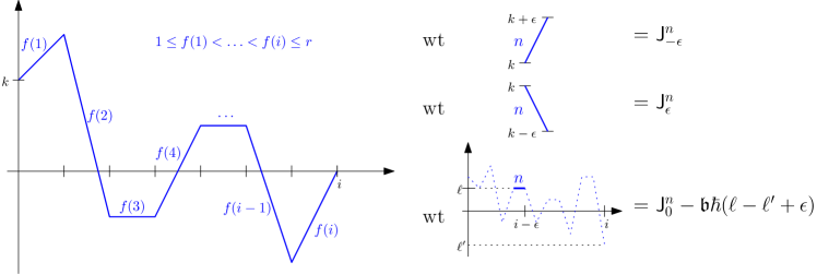
Figure 1. Generic colored path associated with the operators $\mathsf{W}^{i}_{k}$ by (17). Here $k=2,i=7$, and the associated weight is equal to $\mathsf{J}^{f(1)}_{-1}\mathsf{J}^{f(2)}_{4}(\mathsf{J}^{f(3)}_{0}-3\mathfrak{b}\hbar)\mathsf{J}^{f(4)}_{-2}(\mathsf{J}^{f(5)}_{0}-3\mathfrak{b}\hbar)\mathsf{J}^{f(6)}_{3}\mathsf{J}^{f(7)}_{-2}$.

With this set up, we can prove the following combinatorial formula for the modes $\mathsf{W}^{i}_{k}$.

Lemma 3.5.

We have the following combinatorial interpretation of the modes $\mathsf{W}^{i}_{k}$ for all $1\leq i\leq r$ and for all $k\in\mathbb{Z}$:

(17) $$\mathsf{W}^{i}_{k}=\sum_{\begin{subarray}{c}\gamma\in\Gamma_{(0,k)\to(i,0)},\\ f\in\mathcal{F}_{<}([i],[r])\end{subarray}}\operatorname{wt}(\gamma,f),$$

where we recall that $f\in\mathcal{F}_{<}([i],[r])$ means that we are summing over strictly increasing colorings.

Proof.

In this proof, we will need to work with the algebra $\mathcal{W}^{\mathsf{k}}(\mathfrak{gl}_{r-1})$ realized as an embedding into the Heisenberg VOA generated by the fields $\mathsf{J}^{2}(z),\ldots,\mathsf{J}^{r}(z)$. Then the algebra $\mathcal{W}^{\mathsf{k}}(\mathfrak{gl}_{r-1})$ is generated by $(r-1)$ generators, say $\mathsf{W}^{i,r-1}(z)$, defined by the following Miura transform:

$$\sum_{i=0}^{r-1}\mathsf{W}^{i,r-1}(z)(\hbar\mathfrak{b}\partial_{z})^{r-1-i}:=(\hbar\mathfrak{b}\partial_{z}+\mathsf{J}^{2}(z))\cdots(\hbar\mathfrak{b}\partial_{z}+\mathsf{J}^{r}(z))\,.$$

In this proof, we denote the generators of $\mathcal{W}^{\mathsf{k}}(\mathfrak{gl}_{r})$ given by the Miura transform (16) as $\mathsf{W}^{i,r}(z)$, to emphasize the $r$-dependence and avoid confusion. Then, the quantum Miura transform for $\mathcal{W}^{\mathsf{k}}(\mathfrak{gl}_{r})$ can be written as

$$\sum_{i=0}^{r}{\mathsf{W}}^{i,r}(z)(\hbar\mathfrak{b}\partial_{z})^{r-i}=\left(\hbar\mathfrak{b}\partial_{z}+\mathsf{J}^{1}(z)\right)\cdot\sum_{i=0}^{r-1}\mathsf{W}^{i,r-1}(z)(\hbar\mathfrak{b}\partial_{z})^{r-1-i},$$

which, in terms of the modes, gives

(18) $${\mathsf{W}}^{i,r}_{k}=\mathsf{W}^{i,r-1}_{k}+\sum_{k_{1}+k_{2}=k}\left(\mathsf{J}^{1}_{k_{1}}-\delta_{k_{1},0}\hbar\mathfrak{b}(k_{2}+i-1)\right)\cdot\mathsf{W}^{i-1,r-1}_{k_{2}}.$$

In addition to our existing convention that $\mathsf{W}^{0,r}_{k}=\delta_{k,0}$, we set $\mathsf{W}^{r,r-1}_{k}=0$ and $\mathsf{W}^{-1,r-1}_{k}=0$ for any $k\in\mathbb{Z}$.

With this setup, we can prove (17) by induction with respect to the lexicographic order on $(i,r)$. It is clear that the formula holds for $(1,r)$ for all $r$. Assume that it is true for all $(i^{\prime},r^{\prime})<(i,r)$. Then, the RHS of (17) can be decomposed into two terms – either the first step is colored by $f(1)=1$, or $f(1)>1$. When $f(1)=1$, the weight $\operatorname{wt}_{1}(\gamma,f)=\mathsf{J}^{1}_{k_{1}}-\delta_{k_{1},0}\mathfrak{b}\hbar\big{(}k_{2}+i-1\big{)}$, where the first step of $\gamma$ ends at $(1,k_{2})$ and $k_{1}=k-k_{2}$. This gives the following formula for the RHS of (17):

(19) $$\sum_{\begin{subarray}{c}\gamma\in\Gamma_{(0,k)\to(i,0)},\\ f\in\mathcal{F}_{<}([i],[2..r])\end{subarray}}\operatorname{wt}(\gamma,f)+\sum_{k_{1}+k_{2}=k}\left(\mathsf{J}^{1}_{k_{1}}-\delta_{k_{2},0}\hbar\mathfrak{b}(k_{2}+i-1)\right)\cdot\sum_{\begin{subarray}{c}\tilde{\gamma}\in\Gamma_{(0,k_{2})\to(i-1,0)},\\ \tilde{f}\in\mathcal{F}_{<}([i-1],[2..r])\end{subarray}}\operatorname{wt}(\tilde{\gamma},\tilde{f}),$$

where $\tilde{\gamma}$ is the path obtained from $\gamma$ by removing the first step and shifting it one unit to the left, so that $\tilde{\gamma}$ starts at $(0,k_{2})$. Note that the weight of a path is invariant under a horizontal shift. For $j>1$, we define $\tilde{f}(j-1):=f(j)$ such that $\operatorname{wt}_{j}(\gamma,f)=\operatorname{wt}_{j-1}(\tilde{\gamma},\tilde{f})$. The inductive hypothesis gives us the following formula for $j\leq i$:

$$\mathsf{W}^{j,r-1}_{k}=\sum_{\begin{subarray}{c}\gamma\in\Gamma_{(0,k)\to(j,0)},\\ f\in\mathcal{F}_{<}([j],[2..r])\end{subarray}}\operatorname{wt}(\gamma,f),$$

and hence (19) is equivalent to the recursion (18), which finishes the proof. ∎

3.2.2. Algebra of modes

In order to construct an Airy structure, we will need to work with the algebra of modes of the vertex algebra $\mathcal{W}^{\mathsf{k}}(\mathfrak{gl}_{r})$. We consider the algebra $\mathcal{A}^{\hbar}$, which is a suitable completion of the algebra of modes, with the parameter $\hbar$ keeping track of the conformal dimension of the generating fields (see [BBCC21, Section 3.1] for a definition).

The strategy to find an Airy structure is to pick a set of modes of $\mathcal{W}^{\mathsf{k}}(\mathfrak{gl}_{r})$, such that the ideal generated by these modes will be a subalgebra of $\mathcal{A}^{\hbar}$. In addition, we may want to pick a subset of these modes, and shift them to obtain Whittaker vectors. Various such subsets of modes were studied in [BBC⁺18], and we present one of these subsets that is relevant for us. In fact, we prove an upgraded version that allows us to shift the zero modes $\mathsf{W}^{i}_{0}$ later on.

Lemma 3.6.

Consider the set of modes $S$ defined as

$$S:=\left\{\mathsf{W}^{i}_{k}:i\in[r]\,,k\geq 0\right\},$$

and the subset of modes $S^{\prime}:=\left\{\mathsf{W}^{i}_{k}:i\in[r]\,,k\geq 1\right\}\subset S$. Then, for any two modes $\mathsf{W}^{i_{1}}_{k_{1}},\mathsf{W}^{i_{2}}_{k_{2}}$ in $S$, we have

$$[\mathsf{W}^{i_{1}}_{k_{1}},\mathsf{W}^{i_{2}}_{k_{2}}]\in\hbar^{2}\mathcal{A}^{\hbar}\cdot S^{\prime}.$$

Proof.

The weaker statement that $[\mathsf{W}^{i_{1}}_{k_{1}},\mathsf{W}^{i_{2}}_{k_{2}}]\in\hbar^{2}\mathcal{A}^{\hbar}\cdot S$ is a direct application of [BBC⁺18, Proposition 3.14] to the strong generators of $\mathcal{W}^{\mathsf{k}}(\mathfrak{gl}_{r})$ (up to the rescaling by $\hbar$).

To prove the lemma, we need to show that terms appearing in the commutator $[\mathsf{W}^{i_{1}}_{k_{1}},\mathsf{W}^{i_{2}}_{k_{2}}]$ can be ordered such that the rightmost mode of each monomial is not $\mathsf{W}^{i}_{0}$. Using Li’s filtration [Li05], any monomial can be normally ordered to take the form (up to a constant prefactor)

$$\mathsf{W}^{j_{1}}_{\ell_{1}}\cdots\mathsf{W}^{j_{n}}_{\ell_{n}},$$

for some $n\geq 1$, where $\ell_{n}=\max(\ell_{1},\dots,\ell_{n})$ and $\ell_{1}+\cdots+\ell_{n}=k_{1}+k_{2}$. If $k_{1}+k_{2}\geq 1$, we must have $\ell_{n}\geq 1$, and thus the zero modes do not appear as the rightmost mode in the monomial.

For the case $k_{1}=k_{2}=0$, we need to use the fact that the Zhu algebra of $\mathcal{W}^{\mathsf{k}}(\mathfrak{gl}_{r})$ is commutative [Ara17, Theorem 4.16.3]. Recall that the Zhu algebra in general is defined as a certain quotient of the algebra of zero modes [Ara17, Section 3.12]. In the case of $\mathcal{W}^{\mathsf{k}}(\mathfrak{gl}_{r})$, the Zhu algebra is generated by monomials of the form $\mathsf{W}^{i_{1}}_{k_{1}}\cdots\mathsf{W}^{i_{n}}_{k_{n}}$ such that $\sum_{i=1}^{n}k_{i}=0$, modulo relations $\mathsf{W}^{j_{1}}_{\ell_{1}}\cdots\mathsf{W}^{j_{n}}_{\ell_{n}}\cdot\mathsf{W}^{j_{n+1}}_{\ell_{n+1}}\cdots\mathsf{W}^{j_{n+m}}_{\ell_{n+m}}=0$ whenever $\sum_{i=1}^{n}\ell_{i}=-\sum_{j=n+1}^{n+m}\ell_{j}<0$.

Then, we know that the commutator $[\mathsf{W}^{i_{1}}_{0},\mathsf{W}^{i_{2}}_{0}]$ is a linear combination of terms of the form $\mathsf{W}^{j_{1}}_{\ell_{1}}\cdots\mathsf{W}^{j_{n}}_{\ell_{n}}\cdot\mathsf{W}^{j_{n+m}}_{\ell_{n+1}}\cdots\mathsf{W}^{j_{n+m}}_{\ell_{n+m}}$, where $\sum_{i=1}^{n}\ell_{i}=-\sum_{j=n+1}^{n+m}\ell_{j}<0$. Again using Li’s filtration, we can order $\mathsf{W}^{j_{n+1}}_{\ell_{n+1}}\cdots\mathsf{W}^{j_{n+1}}_{\ell_{n+m}}$ such that $\ell_{n+m}>0$, and hence we are done. ∎

3.3. An Airy structure for weighted $b$-Hurwitz numbers

Now that we have introduced the notion of Airy structures and the algebra $\mathcal{W}^{\mathsf{k}}(\mathfrak{gl}_{r})$, we can go ahead and construct the Airy structures we are after. We will consider a specific representation of the vertex algebra $\mathcal{W}^{\mathsf{k}}(\mathfrak{gl}_{r})$, look at a certain subset of modes and prove that they form an Airy structure. This Airy structure will turn out to have a trivial partition function i.e. $Z=1$, but by doing appropriate shifts, we will obtain a shifted Airy structure with an interesting partition function.

Remark 3.7.

It may help the reader to keep in mind that the partition function of the shifted Airy structure that we will eventually construct will be related to the generating function of weighted $b$-Hurwitz numbers with the following weight:

$$G(z)=\frac{\prod_{i=1}^{r}(P_{i}+z)}{\prod_{i=1}^{r-2}(Q_{i}-z)}\,$$

where $r\geq 2$ is an integer. While this is not the most general weight we are interested in, one can take appropriate limits to reduce to an arbitrary rational weight (see Section 4.3.2 for a more detailed explanation).

We will first construct a representation of the Heisenberg VOA $\mathcal{H}_{r}$. Consider the ring $R=\mathbb{C}(\mathbf{P},\mathbf{Q},\mathfrak{b})[\mathbf{x}]$, which is the polynomial ring in infinitely many variables $\mathbf{x}=\{x^{a}_{k}\}_{k\geq 1,a\in[r]}$ over the field of rational functions in $\mathfrak{b}$, $\mathbf{P}=\{P_{1},\dots,P_{r}\}$ and $\mathbf{Q}=\{Q_{0},Q_{1},\dots,Q_{r-2}\}$ — we will set $Q_{0}=0$ in Section 4. Consider the vector space

$$\widehat{\mathcal{M}}:=\prod_{n\in\mathbb{Z}_{\geq 0}}\hbar^{n}\left(R_{\leq n}\right),$$

where $R_{\leq n}$ denotes polynomials in the $x^{a}_{k}$ of degree $\leq n$. A typical element of $\widehat{\mathcal{M}}$ is of the form $\sum_{n=0}^{\infty}\hbar^{n}P_{n}$, where $P_{n}$ is a polynomial in the $x^{a}_{k}$ of degree at most $n$. This vector space $\widehat{\mathcal{M}}$ is a module for the Heisenberg VOA via the following mode assignment:

(20) $$\begin{split}\mathsf{J}^{a}_{k}=\left\{\begin{array}[]{lr}\hbar\partial_{x^{a}_{k}}&k>0,\\ \hbar(-k)x^{a}_{-k}+(-1)^{r}\frac{1}{\Lambda}\delta_{k,-1}\delta_{a,r}&k<0,\\ Q_{a-1}-\hbar\mathfrak{b}(a-1)&a\in[r-1],k=0\\ -\sum_{a^{\prime}=1}^{r}P_{a^{\prime}}-\sum_{a^{\prime}=0}^{r-2}Q_{a^{\prime}}-\hbar\mathfrak{b}(a-1)&a=r,k=0,\\ \end{array}\right.\end{split}$$

Note that while the $\mathsf{J}^{1}_{k}$ have been defined previously in (3), it is not a conflict of notation as we will eventually substitute $\tilde{p}_{k}=kx^{1}_{k}$ (see Theorem 4.7). As the quantum Miura transformation gives an embedding $\mathcal{W}^{\mathsf{k}}(\mathfrak{gl}_{r})\hookrightarrow\mathcal{H}_{r}$, $\widehat{\mathcal{M}}$ is also a module for $\mathcal{W}^{\mathsf{k}}(\mathfrak{gl}_{r})$ by restriction. By abuse of notation, we will henceforth use both $\mathsf{W}^{i}_{k}$ and $\mathsf{J}^{a}_{k}$ to denote the modes of the generators of $\mathcal{W}^{\mathsf{k}}(\mathfrak{gl}_{r})$ and $\mathcal{H}_{r}$, respectively, in the representation $\widehat{\mathcal{M}}$.

We would like to claim that the set of operators $\left\{\mathsf{W}^{i}_{k}:i\in[r],k\geq\delta_{i,1}\right\}$ in the representation $\widehat{\mathcal{M}}$ generates an Airy structure. However, this set of operators does not satisfy condition $(c)$ of Definition 3.1 of Airy structures. Indeed, for an operator $P$ in $\widehat{\mathcal{D}}_{A}^{\hbar}$, let $\pi_{i}(P):=\hbar^{i}\cdot[\hbar^{i}]P$ denote the $\hbar$-degree $i$ term of $P$. Then we have the following two problems: first $\pi_{0}(\mathsf{W}^{i}_{0})\neq 0$, and second $\pi_{1}(\mathsf{W}^{i}_{k})\neq\hbar\partial_{x^{\bullet}_{\bullet}}$.

To address the first issue, let us define new operators $\widetilde{\mathsf{W}}^{i}_{k}$, where we remove some terms by hand, including all the $\hbar$-degree zero terms. Define $\mathsf{V}^{i}$ for any $i\in[r]$ as the following combinations of the Heisenberg zero modes:

$$\mathsf{V}^{i}:=\sum_{f\in\mathcal{F}_{<}([i],[r])}\big{(}\mathsf{J}^{f(1)}_{0}-\hbar\mathfrak{b}(i-1)\big{)}\cdots\big{(}\mathsf{J}^{f(i-1)}_{0}-\hbar\mathfrak{b}\big{)}\mathsf{J}^{f(i)}_{0}.$$

Define, for any $i\in[r]$, and any $k\geq 0$,

(21) $$\widetilde{\mathsf{W}}^{i}_{k}:=\mathsf{W}^{i}_{k}-\mathsf{V}^{i}\delta_{k,0}.$$

To address the second issue, we need to diagonalize the set of operators $\left\{\widetilde{\mathsf{W}}^{i}_{k}:i\in[r],k\geq\delta_{i,1}\right\}$. Assuming that $Q_{0},Q_{1},\dots,Q_{r-2}$ are pairwise distinct, define operators $\widetilde{\mathsf{H}}^{a}_{k}$, for any $a\in[r]$ and any $k\geq 1$:

(22) $$\widetilde{\mathsf{H}}^{r}_{k}:=\widetilde{\mathsf{W}}^{1}_{k}+\sum_{a\neq r}\sum_{\ell=0}^{k-1}\frac{((-1)^{r}\Lambda)^{\ell+1}\left(-e_{1}(\mathbf{P})-e_{1}(\mathbf{Q})-Q_{a-1}\right)^{\ell}}{\prod_{a^{\prime}\neq a,r}\left(Q_{a^{\prime}-1}-Q_{a-1}\right)}\sum_{i=1}^{r}(-Q_{a-1})^{r-i}\widetilde{\mathsf{W}}^{i}_{k-1-\ell}\,$$ .

$$\widetilde{\mathsf{H}}^{a}_{k}:=-\sum_{\ell=0}^{k-1}\frac{((-1)^{r}\Lambda)^{\ell+1}\left(-e_{1}(\mathbf{P})-e_{1}(\mathbf{Q})-Q_{a-1}\right)^{\ell}}{\prod_{a^{\prime}\neq a,r}\left(Q_{a^{\prime}-1}-Q_{a-1}\right)}\sum_{i=1}^{r}(-Q_{a-1})^{r-i}\widetilde{\mathsf{W}}^{i}_{k-1-\ell},\ \text{ for }a\in[r-1]$$ .

These operators $\widetilde{\mathsf{H}}^{a}_{k}$ are diagonal in the following sense.

Lemma 3.8.

For any $1\leq a\leq r$ and $k\geq 1$, we have

$$\widetilde{\mathsf{H}}^{a}_{k}=\hbar\partial_{x^{a}_{k}}+O(\hbar^{2})\,.$$

Proof.

First notice that $\pi_{0}(\mathsf{J}^{a}_{k})=0$ for all $k>0$. Lemma 3.5 implies that $\mathsf{W}^{i}_{k}$ can be written as a linear combination of operators associated with colored paths and the only paths in (17) that contribute in $\hbar$-degree zero are paths that do not have any steps of negative increment. Since $k\geq 0$, the only such path appears when $k=0$ and it is the path that runs horizontally from $(0,0)$ to $(i,0)$. Therefore (17) implies that

$$\mathsf{W}^{i}_{k}=\delta_{k,0}\sum_{f\in\mathcal{F}_{<}([i],[r])}\big{(}\mathsf{J}^{f(1)}_{0}-\hbar\mathfrak{b}(i-1)\big{)}\cdots\big{(}\mathsf{J}^{f(i-1)}_{0}-\hbar\mathfrak{b}\big{)}\mathsf{J}^{f(i)}_{0}+O(\hbar)=\delta_{k,0}\mathsf{V}^{i}+O(\hbar),$$

which further implies that $\pi_{0}(\widetilde{\mathsf{W}}^{i}_{k})=0$. Similarly, the only paths in (17) that contribute in $\hbar$-degree one are paths that have precisely one step of negative increment. Moreover, $\pi_{0}(\mathsf{J}^{a}_{k})=0$ for all $k<0$ except for $a=r$ and $k=-1$. Therefore the only paths in (17) that contribute in $\hbar$-degree one are paths that have precisely one step of negative increment – either they finish with a step from $(i-1,-1)$ to $(i,0)$ colored by $r$, or they have precisely one step of negative increment and all the other steps are flat. Thus, (17) implies that the corresponding $\hbar$-degree one part is given by

$$\pi_{1}(\widetilde{\mathsf{W}}^{i}_{k})=\frac{(-1)^{r}}{\Lambda}\sum_{a=1}^{r-1}\hbar\partial_{x^{a}_{k+1}}\pi_{0}(e_{i-2}(\mathsf{J}^{1}_{0},\dots,\hat{\mathsf{J}^{a}_{0}},\dots,\mathsf{J}^{r-1}_{0}))+\sum_{a=1}^{r}\hbar\partial_{x^{a}_{k}}\pi_{0}(e_{i-1}(\mathsf{J}^{1}_{0},\dots,\hat{\mathsf{J}^{a}_{0}},\dots,\mathsf{J}^{r}_{0}))\delta_{k>0},$$

for any $i\in[r]$ and $k\geq 0$. In generating series form, we can express this formula as

$$\sum_{i=1}^{r}u^{r-i}\pi_{1}(\widetilde{\mathsf{W}}^{i}_{k})=\frac{(-1)^{r}}{\Lambda}\sum_{a=1}^{r-1}\hbar\partial_{x^{a}_{k+1}}\prod_{a^{\prime}\neq a,r}(u+\pi_{0}(\mathsf{J}^{a^{\prime}}_{0}))+\sum_{a=1}^{r}\hbar\partial_{x^{a}_{k}}\prod_{a^{\prime}\neq a}(u+\pi_{0}(\mathsf{J}^{a^{\prime}}_{0}))\delta_{k>0}\,.$$

For any $a\neq r$ we can invert it by dividing by $\prod_{a^{\prime}=1}^{r}(u+\pi_{0}(\mathsf{J}^{a^{\prime}}_{0}))$ and taking the residue at $u=-\pi_{0}(\mathsf{J}^{a}_{0})$, which for $k\geq 0$ gives

(23) $$\frac{-(-1)^{r}\Lambda\pi_{0}(\mathsf{J}^{r}_{0}-\mathsf{J}^{a}_{0})}{\prod_{a^{\prime}\neq a}\pi_{0}(\mathsf{J}^{a^{\prime}}_{0}-\mathsf{J}^{a}_{0})}\sum_{i=1}^{r}(-\pi_{0}(\mathsf{J}^{a}_{0}))^{r-i}\pi_{1}(\widetilde{\mathsf{W}}^{i}_{k})=\hbar\partial_{x^{a}_{k+1}}+(-1)^{r}\Lambda\pi_{0}(\mathsf{J}^{r}_{0}-\mathsf{J}^{a}_{0})\hbar\partial_{x^{a}_{k}}\delta_{k>0}.$$

We complete diagonalization by removing the term $(-1)^{r}\Lambda\hbar\partial_{x^{a}_{k}}\pi_{0}(\mathsf{J}^{r}_{0}-\mathsf{J}^{a}_{0})\delta_{k>0}$ on the RHS of (23), which leads to the definition of $\widetilde{\mathsf{H}}^{a}_{k}$ for $a\neq r$ by comparing with (20). When $a=r$, and $k\geq 1$ we have $\mathsf{J}^{r}_{k}=\widetilde{\mathsf{W}}^{1}_{k}-\sum_{a=1}^{r-1}\mathsf{J}^{a^{\prime}}_{k}$ for any $k\geq 1$, hence we define $\widetilde{\mathsf{H}}^{r}_{k}=\widetilde{\mathsf{W}}^{1}_{k}-\sum_{a^{\prime}=1}^{r-1}\widetilde{\mathsf{H}}^{a^{\prime}}_{k}$. ∎

Finally, we are ready to construct an Airy structure.

Proposition 3.9.

Assume that $Q_{0},Q_{1},\dots,Q_{r-2}$ are pairwise distinct. Then, the ideal $\mathcal{I}$ generated by the set of operators

$$\widetilde{\mathsf{W}}^{i}_{k}\qquad\text{ for }i\in[r]\,,\,k\geq\delta_{i,1}$$

is an Airy structure.

Proof.

We will work with the diagonalized set of operators $\widetilde{\mathsf{H}}^{a}_{k}$ as defined in (22). The set of operators

(24) $$\left\{\widetilde{\mathsf{H}}^{a}_{k}:a\in[r]\,,k\geq 1\right\}$$

also generate the ideal $\mathcal{I}$ as the change of basis (22) is invertible.

We need to check the conditions $(a)-(d)$ to be an Airy structure from Definition 3.1.

1. The operators $\widetilde{\mathsf{W}}^{i}_{k}$ are bounded by [BCJ22, Lemma 2.43], which proves that any set of non-negative modes of a vertex algebra obtained from a representation of a Heisenberg VOA is bounded. The operators $\widetilde{\mathsf{H}}^{a}_{k}$ are also bounded as they are finite linear combinations of the $\widetilde{\mathsf{W}}^{i}_{k}$.

2. As we mentioned at the start of the proof, the ideal $\mathcal{I}$ is generated by the set of operators (24).

3. $\widetilde{\mathsf{H}}^{a}_{k}=\hbar\partial_{x^{a}_{k}}+O(\hbar^{2})$ by Lemma 3.8.

4. Lemma 3.6 shows that the ideal generated by the set of operators $\left\{\mathsf{W}^{i}_{k}:i\in[r],k\geq 0\right\}$ satisfies condition $(d)$ to be an Airy structure. In fact, it also allows us to shift the subset of operators $\{\mathsf{W}^{i}_{0}:i\in[r]\}$ to get the subset $\{\widetilde{\mathsf{W}}^{i}_{0}:i\in[r]\}$, and the ideal $\mathcal{I}$ generated by the resulting operators will still satisfy condition $(d)$. (Note that $\widetilde{\mathsf{W}}^{1}_{0}=0$, and hence we may disregard it.) ∎

While we have constructed an Airy structure, the partition function associated to it can easily seen to be trivial. As we know that there is a unique solution by Theorem 3.3 all that needs to be done is to check that $Z=1$ is a solution to the set of equations

$$\mathsf{W}^{i}_{k}Z=\mathsf{V}^{i}\delta_{k,0}Z\qquad\text{ for }i\in[r]\,,\,k\geq\delta_{i,1}\,.$$

As this is a straightforward check, and we do not need this result in this paper, we leave it as an exercise for the interested reader.

3.3.1. Shifted Airy structure

In order to get the partition function that we are interested in, we need to shift the zero modes $\mathsf{W}^{i}_{0}$. More precisely, we have the following theorem.

Theorem 3.10.

Assume that $Q_{0},Q_{1},\dots,Q_{r-2}$ are pairwise distinct. Then, the ideal $\mathcal{I}^{L}$ generated by the set of operators

(25) $$\mathsf{W}^{i}_{k}-\mathsf{V}^{i}\delta_{k,0}-L_{i}\delta_{k,0}\qquad\text{ for }i\in[r]\,,\,k\geq\delta_{i,1}\,,$$

where $\left(L_{i}\right)_{i\in[2..r]}$ are formal commuting variables of $\deg_{\hbar}L_{i}=0$, is a shifted Airy structure.

Proof.

We know from Proposition 3.9, that the ideal generated by the operators $\mathsf{W}^{i}_{k}-\mathsf{V}^{i}\delta_{k,0}$ is an Airy structure. So all we need to check to get a shifted Airy structure is that the condition $[\mathcal{I}^{L},\mathcal{I}^{L}]\subseteq\hbar^{2}\mathcal{I}^{L}$ is satisfied. Lemma 3.6 does the job, as it says that the modes $\mathsf{W}^{i}_{0}$ can be shifted freely without changing the commutation relations. ∎

Recall that by Theorem 3.3 of Airy structures, the shifted Airy structure $\mathcal{I}^{L}$ has a unique partition function, say $\mathcal{Z}^{L}$ of the following form:

$$\mathcal{Z}^{L}=\exp\left(\sum_{\begin{subarray}{c}g\in\frac{1}{2}\mathbb{Z}_{\geq 0},n\in\mathbb{Z}_{>0}\end{subarray}}\hbar^{2g-2+n}F_{g,n}\right)\,$$

where the $F_{g,n}$, a priori, are elements of $\mathbb{C}(\!(\mathbf{P},\mathbf{Q},\Lambda)\!)(\mathfrak{b})[\mathbf{x}]\llbracket L_{2},\ldots,L_{r}\rrbracket$, and in this case the partition function $\mathcal{Z}^{L}$ will indeed be non-trivial.

We need to study the properties of the partition function $\mathcal{Z}^{L}$, especially the dependence of the $F_{g,n}$ on the $L_{i}$, as we will want to specialize the $L_{i}$ to functions of $\mathbf{P}$ and $\mathfrak{b}$ later on (see (29)). Let us define the expansion coefficients of $F_{g,n}$ as follows:

$$F_{g,n}=\frac{1}{n!}\sum_{\begin{subarray}{c}a_{1},\ldots,a_{n}\in[r]\\ k_{1},\ldots,k_{n}\in\mathbb{Z}_{>0}\end{subarray}}F_{g,n}\big{[}\begin{smallmatrix}a_{1}&\cdots&a_{n}\\ k_{1}&\cdots&k_{n}\end{smallmatrix}\big{]}\prod_{i=1}^{n}x^{a_{i}}_{k_{i}}.$$

such that $F_{g,n}\big{[}\begin{smallmatrix}a_{1}&\cdots&a_{n}\\ k_{1}&\cdots&k_{n}\end{smallmatrix}\big{]}$ is an element of $\mathbb{C}(\!(\mathbf{P},\mathbf{Q},\Lambda)\!)(\mathfrak{b})\llbracket L_{2},\ldots,L_{r}\rrbracket$. We can show that the $F_{g,n}\big{[}\begin{smallmatrix}a_{1}&\cdots&a_{n}\\ k_{1}&\cdots&k_{n}\end{smallmatrix}\big{]}$ actually live in $\mathbb{Q}(\mathbf{Q})[\mathbf{P},\mathfrak{b},\Lambda][L_{2},\ldots,L_{r}]$:

Proposition 3.11.

The $F_{g,n}\big{[}\begin{smallmatrix}a_{1}&\cdots&a_{n}\\ k_{1}&\cdots&k_{n}\end{smallmatrix}\big{]}$ of the partition function depend polynomially on $\Lambda,\mathfrak{b},\mathbf{P}$ and $L_{2},\cdots,L_{r}$ and rationally on $\mathbf{Q}$. More precisely, we have

$$\frac{F_{g,n}\big{[}\begin{smallmatrix}a_{1}&\cdots&a_{n}\\ k_{1}&\cdots&k_{n}\end{smallmatrix}\big{]}}{\Lambda^{k_{1}+\cdots+k_{n}}}\in\mathbb{Q}(\mathbf{Q})[\mathbf{P},\mathfrak{b}][L_{2},\ldots,L_{r}].$$

Proof.

In this proof we will denote by $(I|A)$ a tuple of two ordered sets $I=\{i_{1},\dots,i_{d}\}\subset\mathbb{Z}^{d}_{>0}$, and $A=\{a_{1},\dots,a_{d}\}\subset[r]^{d}$ of the same cardinality $|(I|A)|:=d$. For such a tuple we denote $\mathbf{x}^{A}_{I}:=\prod_{j=1}^{|A|}x_{i_{j}}^{a_{j}}$, and $\partial_{\mathbf{x}^{A}_{I}}:=\prod_{j=1}^{|A|}\partial_{x_{i_{j}}^{a_{j}}}$. Equations (17), (20), and (21) imply that

$$\Lambda\widetilde{\mathsf{W}}_{k}^{i}=\sum_{d+h=1}^{i}\sum_{|(I_{1}|A_{1})\sqcup(I_{2}|A_{2})|=d}\hbar^{h}K_{k,h}^{i}\big{[}\begin{smallmatrix}{A}_{1}&{A}_{2}\\ {I}_{1}&{I}_{2}\end{smallmatrix}\big{]}\cdot\hbar^{d}\cdot\mathbf{x}^{A_{1}}_{I_{1}}\cdot\partial_{\mathbf{x}^{A_{2}}_{I_{2}}},$$

where $K_{k,h}^{i}\big{[}\begin{smallmatrix}{A}_{1}&{A}_{2}\\ {I}_{1}&{I}_{2}\end{smallmatrix}\big{]}\in\mathbb{Q}[\mathbf{P},\mathbf{Q},\mathfrak{b},\Lambda]$ vanish unless $\sum_{i^{\prime\prime}\in{I}_{2}}i^{\prime\prime}-\sum_{i^{\prime}\in{I}_{1}}i^{\prime}\leq k+1$. Therefore (22) and Lemma 3.8 further imply that

(26) $$\hbar\partial_{x_{k}^{a}}=\widetilde{\mathsf{H}}_{k}^{a}+\sum_{d+h=2}^{r}\sum_{|(I_{1}|A_{1})\sqcup(I_{2}|A_{2})|=d}\hbar^{h}U_{k,h}^{a}\big{[}\begin{smallmatrix}{A}_{1}&{A}_{2}\\ {I}_{1}&{I}_{2}\end{smallmatrix}\big{]}\cdot\hbar^{d}\cdot\mathbf{x}^{A_{1}}_{I_{1}}\cdot\partial_{\mathbf{x}^{A_{2}}_{I_{2}}},$$

where $U_{k,h}^{a}\big{[}\begin{smallmatrix}{A}_{1}&{A}_{2}\\ {I}_{1}&{I}_{2}\end{smallmatrix}\big{]}\in\mathbb{Q}(\mathbf{Q})[\mathbf{P},\mathfrak{b},\Lambda]$ vanish unless $\sum_{i^{\prime\prime}\in{I}_{2}}i^{\prime\prime}-\sum_{i^{\prime}\in{I}_{1}}i^{\prime}\leq k$. Moreover (22) together with the shifted Airy structure (25) gives that

(27) $$\frac{1}{\mathcal{Z}^{L}}\widetilde{\mathsf{H}}_{k}^{a}\mathcal{Z}^{L}=\widetilde{U}_{k}^{a}\in\Lambda^{k}\cdot\mathbb{Q}(\mathbf{Q})[\mathbf{P},L_{2},\dots,L_{r}]$$

for any $a\in[r],k\geq 1$, where the coefficients $\widetilde{U}_{k}^{a}$ can be written explicitly from (22).

Note that we can extract the coefficients of $\mathcal{Z}^{L}$ as follows

$$F_{g,n}\big{[}\begin{smallmatrix}a_{1}&\cdots&a_{n}\\ k_{1}&\cdots&k_{n}\end{smallmatrix}\big{]}=[\hbar^{2g-1+n}]\left(\prod_{l=2}^{n}\partial_{x_{k_{l}}^{a_{l}}}\frac{1}{\mathcal{Z}^{L}}(\hbar\partial_{x_{k_{1}}^{a_{1}}})\mathcal{Z}^{L}\right)\Bigg{|}_{\mathbf{x}=0}.$$

Applying (26) with $k=k_{1},a=a_{1}$, and comparing it with (27), we obtain the following identity

$$F_{g,n}\big{[}\begin{smallmatrix}a_{1}&\cdots&a_{n}\\ k_{1}&\cdots&k_{n}\end{smallmatrix}\big{]}=\delta_{n,1}\delta_{g,0}\widetilde{U}_{k_{1}}^{a_{1}}+ \sum_{d+h=2}^{r}\sum_{l=1}^{d}\sum_{\begin{subarray}{c}|(I|A)\sqcup(I_{1}|A_{1})\sqcup\cdots\sqcup(I_{l}|A_{l})|=d,\\ |(I_{1}|A_{1})|,\cdots,|(I_{l}|A_{l})|\geq 1\end{subarray}}\cdot$$

(28) $$\sum_{\begin{subarray}{c}(I^{\prime}_{1}|A^{\prime}_{1})\sqcup\cdots\sqcup(I^{\prime}_{l}|A^{\prime}_{l})\sqcup({I}|{A})=\\ =(\{k_{2},\dots,k_{n}\}|\{a_{2},\dots,a_{n}\})\end{subarray}} \sum_{\begin{subarray}{c}g_{1},\cdots,g_{l}\in\frac{1}{2}\mathbb{Z}_{>0},\\ 2\sum_{m}(g_{m}-1+|{I}_{m}|)=2g-h\end{subarray}}U_{k_{1},h}^{a_{1}}\big{[}\begin{smallmatrix}{A}&{A}_{1}\cdots{A}_{l}\\ {I}&{I}_{1}\cdots{I}_{l}\end{smallmatrix}\big{]}\prod_{m=1}^{l}F_{g_{m},|I^{\prime}_{m}|+|{I}_{m}|}\big{[}\begin{smallmatrix}A^{\prime}_{m}&{A}_{m}\\ I^{\prime}_{m}&{I}_{m}\end{smallmatrix}\big{]}.$$

While the formula above looks complicated (it follows by applying the Leibnitz rule repeatedly and we leave its verification to the interested reader), we only need the following property: the RHS is a finite combination over $\mathbb{Q}(\mathbf{Q})[\mathbf{P},\mathfrak{b},\Lambda][L_{2},\ldots,L_{r}]$ of products of terms of the form $F_{g^{\prime},n^{\prime}}\big{[}\begin{smallmatrix}a^{\prime}_{1}&\cdots&a^{\prime}_{n^{\prime}}\\ k^{\prime}_{1}&\cdots&k^{\prime}_{n^{\prime}}\end{smallmatrix}\big{]}$ with $2g^{\prime}-2+n^{\prime}\leq 2g-2+n$ and $k^{\prime}_{1}+\cdots+k^{\prime}_{n^{\prime}}\leq k_{1}+\cdots+k_{n}$. Indeed, the condition $\sum_{i\in{I}_{m}}i+\sum_{i^{\prime}\in{I}^{\prime}_{m}}i^{\prime}\leq k_{1}+\cdots+k_{n}$ follows from the vanishing condition for $U_{k_{1},h}^{a_{1}}\big{[}\begin{smallmatrix}{A}&A_{1}\cdots A_{l}\\ {I}&I_{1}\cdots I_{l}\end{smallmatrix}\big{]}$. Similarly,

$$2g_{m}-2+|I^{\prime}_{m}|+|I_{m}|\leq 2\sum_{m}(g_{m}-1+|I_{m}|)+|I^{\prime}_{m}|-|I_{m}|=2g-h+|I^{\prime}_{m}|-|I_{m}|\leq 2g-2+n,$$

and the equality holds if and only if $h=0$, $I^{\prime}_{m}=\{k_{2},\dots,k_{n}\}$ (thus, $I=\emptyset$), $|I_{m}|=1$ and $g_{m}=g$. Since $d\geq 2$ these conditions imply that $l\geq 2$, therefore the vanishing condition for $U_{k_{1},h}^{a_{1}}\big{[}\begin{smallmatrix}{A}&A_{1}\cdots A_{l}\\ {I}&I_{1}\cdots I_{l}\end{smallmatrix}\big{]}$ implies that $I_{m}=\{y\}$ with $y<k_{1}$. Thus, we conclude that for $F_{g^{\prime},n^{\prime}}\big{[}\begin{smallmatrix}a^{\prime}_{1}&\cdots&a^{\prime}_{n^{\prime}}\\ k^{\prime}_{1}&\cdots&k^{\prime}_{n^{\prime}}\end{smallmatrix}\big{]}$ with $2g^{\prime}-2+n^{\prime}=2g-2+n$ we necessarily have a strict inequality $k^{\prime}_{1}+\cdots+k^{\prime}_{n^{\prime}}<k_{1}+\cdots+k_{n}$. Consequently, (28) can be used to compute the $F_{g,n}\big{[}\begin{smallmatrix}a_{1}&\cdots&a_{n}\\ k_{1}&\cdots&k_{n}\end{smallmatrix}\big{]}$ recursively on $K=k_{1}+\cdots+k_{n}$ and then on $\chi=2g-2+n$ in the lexicographic order and the claim $F_{g,n}\big{[}\begin{smallmatrix}a_{1}&\cdots&a_{n}\\ k_{1}&\cdots&k_{n}\end{smallmatrix}\big{]}\in\mathbb{Q}(\mathbf{Q})[\mathbf{P},\mathfrak{b},\Lambda][L_{2},\ldots,L_{r}]$ follows inductively.

To prove the specific form of the dependence on $\Lambda$ let us simultaneously rescale $x^{a}_{k}\mapsto c^{-k}\,x^{a}_{k}$ and $\Lambda\mapsto c\,\Lambda$ for some $c\in\mathbb{C}^{*}$, which corresponds to $\mathsf{J}_{k}^{a}\mapsto c^{k}\mathsf{J}_{k}^{a}$ and $\widetilde{\mathsf{W}}^{i}_{k}\mapsto c^{k}\,\widetilde{\mathsf{W}}^{i}_{k}$. Then, as (25) remains unchanged under this rescaling, so does the solution $\mathcal{Z}^{L}$. Thus, every $F_{g,n}\big{[}\begin{smallmatrix}a_{1}&a_{2}&\cdots&a_{n}\\ k_{1}&k_{2}&\cdots&k_{n}\end{smallmatrix}\big{]}$ is a monomial in $\Lambda$ of degree $k_{1}+\cdots+k_{n}$, which finishes the proof. ∎

As there are only a finite number of positive integers $k_{1},\dots,k_{n}$ with the fixed sum $k_{1}+\cdots+k_{n}=k$, we have the following corollary of Proposition 3.11.

Corollary 3.12.

The expansion coefficients $F_{g,n}$ of the partition function $\mathcal{Z}^{L}$ are elements of the ring $\mathbb{Q}(\mathbf{Q})[\mathbf{P},\mathfrak{b},L_{2},\ldots,L_{r},\mathbf{x}]\llbracket\Lambda\rrbracket$.

4. $b$-Hurwitz numbers from the Airy structure

In this section, we continue the study of the partition function $\mathcal{Z}^{L}$ of the shifted Airy structure. After performing various substitutions, we will prove that $\mathcal{Z}^{L}$ reduces to the generating function $\tau^{(\mathfrak{b})}_{G}$ of weighted $b$-Hurwitz numbers for an arbitrary rational weight $G(z)$. As a consequence, we will prove a stronger set of constraints for $\tau^{(\mathfrak{b})}_{G}$, from which the cut-and-join equation derived in Theorem 2.7 follows.

4.1. Reduction of the Airy structure

Recall that the partition function $\mathcal{Z}^{L}$ depends on the parameters $\mathbf{P},\mathbf{Q},\Lambda,\mathfrak{b},\mathbf{x}$ and the $\left(L_{i}\right)_{i\in[2..r]}$. We will prove that $\mathcal{Z}^{L}$ reduces to $\tau^{(\mathfrak{b})}_{G}$ for the weight $G(z)=\frac{\prod_{i=1}^{r}(P_{i}+z)}{\prod_{i=1}^{r-2}(Q_{i}-z)}$ after the following substitutions:

S1:

set $Q_{0}=0$,

S2:

set all the variables $x^{a}_{k}=0$ unless $a=1$, i.e.,

$$x^{a}_{k}=0,\qquad a\in[2..r],\quad k\in\mathbb{Z}_{\geq 1},$$

S3:

for any $i\in[2..r]$, we set the $L_{i}$ to be the following:

(29) $$L_{i}=\sum_{1\leq n_{1}<\dots<n_{i}\leq r}\prod_{m=1}^{i}\big{(}-P_{r+1-n_{m}}-\hbar\mathfrak{b}(r-n_{m}+m-1)\big{)}-\mathsf{V}^{i}.$$

When $\mathfrak{b}=0$, it is known [BDBKS20] that these $G$-weighted Hurwitz numbers can be obtained by topological recursion on a certain spectral curve of degree $r$ (see Section 5.1 for the explicit form of the curve). This perspective of topological recursion provides the following motivation for the $\mathfrak{b}=0$ part of the substitutions S1–S3.

• The mode $\mathsf{J}_{0}^{a}$ is related to the residue of $\omega_{0,1}$ at the $a$-th preimage of $x^{-1}(\infty)=(0,Q_{1},..,Q_{r-2},\infty)$ from which we expect that $Q_{0}=0$. As the only condition on the Airy structure is that the $Q_{0},\ldots,Q_{r-2}$ are pairwise disjoint, we may impose $Q_{0}=0$, as long as we assume that $Q_{i}\in\mathbb{C}^{*}$ for $i\in[r-2]$.

• For the spectral curve given in Section 5.1, the expansion of the correlators $\omega_{g,n}(z_{1},..,z_{n})$ at $z_{i}=0$ produces the corresponding weighted Hurwitz numbers. On the other hand, [BCU] (see Theorem 5.1) proves that the expansion of $\omega_{g,n}(z_{1},..,z_{n})$ at $z_{i}=0$ is related to the coefficients $F_{g,n}\big{[}\begin{smallmatrix}1&\cdots&1\\ k_{1}&\cdots&k_{n}\end{smallmatrix}\big{]}$ of $\mathcal{Z}^{L}$. In other words, the part of $\mathcal{Z}^{L}$ that survives after setting $x_{k}^{a}=0$ for all $k\geq 1,a\in[2..r]$ gives Hurwitz numbers.

• The choice of $L_{i}$ when $\mathfrak{b}=0$ is again inspired by [BDBKS20] and [BCU], in particular the form of the (global) loop equations.

The above observations do not help determine the $\mathfrak{b}$-dependence of $L_{i}$, because refinements of the results of [BDBKS20, BCU] for arbitrary $\mathfrak{b}$ are still under investigation. The $\mathfrak{b}$-corrections are dictated by the form of the cut-and-join equation from Theorem 2.7 (see Section 4.3.2 for more details).

It is worth emphasizing that the substitution S3 (29) for the $L_{i}$ is allowed as the $F_{g,n}$ is proved to be a polynomial in $L_{i}$ in Corollary 3.12. Thus, after substitution, we will not have arbitrarily negative powers in the $\mathbf{P}$ and $\mathbf{Q}$, and the resulting $F_{g,n}$ will belong to $\mathbb{Q}(\mathbf{Q})[\mathbf{P},\mathfrak{b},\mathbf{x}]\llbracket\Lambda\rrbracket$. We will denote the function obtained after the substitutions S1 and S3 simply by $\mathcal{Z}$, without a superscript. Then, $\mathcal{Z}$ has the form

$$\mathcal{Z}=\exp\left(\sum_{\begin{subarray}{c}g\in\frac{1}{2}\mathbb{Z}_{\geq 0},n\in\mathbb{Z}_{>0}\end{subarray}}\hbar^{2g-2+n}F_{g,n}\right)\,$$

where $F_{g,n}$ is an element of $\mathbb{Q}(\mathbf{Q})[\mathbf{P},\mathfrak{b},\mathbf{x}]\llbracket\Lambda\rrbracket$, and satisfies the constraints

(30) $$\mathsf{W}^{i}_{k}\mathcal{Z}=\Omega_{i}\delta_{k,0}\mathcal{Z}\qquad\text{ for }i\in[r]\,,\,k\geq 0\,,$$

where we define the $\Omega_{i}$ for $i\in[r]$ as

(31) $$\Omega_{i}:=\sum_{1\leq n_{1}<\dots<n_{i}\leq r}\prod_{m=1}^{i}\big{(}-P_{r+1-n_{m}}-\mathfrak{b}\hbar(r-n_{m}+m-1)\big{)}\,.$$

Note that $\mathsf{W}^{1}_{0}=\sum_{a=1}^{r}\mathsf{J}_{0}^{a}=\Omega_{1}$, and hence we have included the (trivial) constraint for $\mathsf{W}^{1}_{0}$ in (30). It will also be convenient in the following to define $\Omega_{0}:=1$. We will refer to the set of equations (30) as $\mathcal{W}$-constraints. We will denote the function obtained after all the substitutions S1–S3 by $\mathcal{Z}^{\operatorname{red}}$, and refer to it as the reduced partition function.

Remark 4.1.

It is important to note that the state $\mathcal{Z}$ satisfying (30) is not the highest weight vector for the representation of ${\mathcal{W}}^{\mathsf{k}}(\mathfrak{gl}_{r})$ that we are considering in this paper. Indeed, the highest weight vector in this representation is the partition function $1$ of the Airy structure $\mathcal{I}$ of Proposition 3.9. This vector $\mathcal{Z}$ is obtained by a shift of the zero modes $\mathsf{W}^{i}_{0}$ and we will refer to it as a Whittaker vector (extending the terminology used in [SV13, BBCC21]).

4.2. Constraints for $\mathcal{Z}^{\operatorname{red}}$

The goal of this section is to find a set of constraints for the reduced partition function $\mathcal{Z}^{\operatorname{red}}$ which will determine it uniquely. Naively, one might want to apply the substitutions S1–S3 directly to the operators $\mathsf{W}^{i}_{k}$ appearing in the $\mathcal{W}$-constraints (30). However, the resulting operators will not annihilate the reduced partition function $\mathcal{Z}^{\operatorname{red}}$. Indeed, the recursive process of solving the $\mathcal{W}$-constraints (30) to obtain $\mathcal{Z}$ mixes together the various $a$, and hence, cannot directly be reduced to a recursive formula purely in terms of the $F_{g,n}\big{[}\begin{smallmatrix}1&\cdots&1\\ k_{1}&\cdots&k_{n}\end{smallmatrix}\big{]}$.

Instead, we find a sequence of different operators $\widehat{D}^{r}_{k}$, defined as certain combinations of the $\mathsf{W}^{i}_{k}$, that annihilate $\mathcal{Z}$. These operators $\widehat{D}^{r}_{k}$ are constructed such that the substitution S2 commutes with the action of $\widehat{D}^{r}_{k}$ on $\mathcal{Z}$. Then the operators $D_{k}$, defined as the reduction of $\widehat{D}^{r}_{k}$ under substitution S2, annihilate $\mathcal{Z}^{\operatorname{red}}$, and are closely related to the cut-and-join equation of Theorem 2.7.

4.2.1. The $\widehat{D}$-operators

As before, we fix an integer $r\geq 2$. Let us begin by defining certain differential operators $\widehat{D}^{i}_{k}$. For $i=0$, we set $\widehat{D}^{0}_{k}:=0$ for any $k\in\mathbb{Z}$. Then we recursively define, for any $i\in[r]$ and $k\in\mathbb{Z}$,

(32) $$\widehat{D}^{i}_{k}:=(-1)^{i+1}(\mathsf{W}^{i}_{k}-\delta_{k,0}\Omega_{i})+\sum_{\begin{subarray}{c}k_{2}\geq 0\\ k_{1}+k_{2}=k\end{subarray}}\left(\mathsf{J}^{1}_{k_{1}}-\delta_{k_{1},0}\hbar\mathfrak{b}(k_{2}+i-1)\right)\widehat{D}^{i-1}_{k_{2}}\,.$$

From the definition of $\Omega_{1}$, it is easy to see that $\widehat{D}^{1}_{0}=0$.

Lemma 4.2.

We have the following constraints for the function $\mathcal{Z}$:

$$\widehat{D}^{i}_{k}\mathcal{Z}=0\qquad\text{ for }i\in[r]\,,\,k\geq 0\,.$$

Proof.

The statement of the lemma follows directly from the the $\mathcal{W}$-constraints of equation (30), and the definition (32) of the operators $\widehat{D}^{i}_{k}$. ∎

In order to prove certain properties of the operators $\widehat{D}^{i}_{k}$, we will find a combinatorial interpretation for them in terms of weighted lattice paths. We will use the combinatorial formula for the operators $\mathsf{W}^{i}_{k}$ in terms of weighted colored paths proved in Lemma 3.5. Recall the notion of bridges from Definition 2.6. Here is a combinatorial formula for the $\widehat{D}$-operators, which is illustrated in Fig. 2.

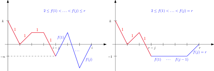
Figure 2. Left: A typical path contributing to the operator $\widehat{D}^{i}_{k}$ from the last sum in (33). Right: A path contributing to the operator $\widehat{D}^{r}_{k}$ from the last sum in (33) that doesn’t vanish after substituting $x^{a}_{k}=0$ for all $a\in[r],k\in\mathbb{Z}_{\geq 1}$. Here the asssociated weight after the substitution is equal to $\mathsf{J}^{1}_{2}\mathsf{J}^{1}_{-1}\mathsf{J}^{1}_{2}(Q_{f(1)-1}-\mathfrak{b}\hbar(f(1)+j-3)\cdots(Q_{f(j)-1}-\mathfrak{b}\hbar(f(j-1)-1)(-1)^{r+1}\Lambda^{-1}$.

Lemma 4.3.

For any $i\in[r]$ and $k\geq 0$, we have the following combinatorial interpretation of the $\widehat{D}$-operators:

$$\widehat{D}^{i}_{k} =(-1)^{i+1}\sum_{\begin{subarray}{c}\gamma\in\Gamma_{(0,k)\to(i,0)},\\ f\in\mathcal{F}_{<}([i],[2..r])\end{subarray}}\operatorname{wt}(\gamma,f)+\sum_{j=0}^{i}\sum_{\gamma\in\Gamma^{\geq 0}_{(0,k)\to(i-j,0)}}(-1)^{j}\Omega_{j}\prod_{u=0}^{i-j}\operatorname{wt}_{u}(\gamma\cup\gamma_{0},\mathbf{1})$$

(33) $$+\sum_{j=1}^{i-1}\sum_{n=1}^{\infty}\sum_{\gamma\in\Gamma^{\geq 0}_{(0,k)\to(i-j,-n)}}\sum_{\begin{subarray}{c}\gamma^{\prime}\in\Gamma_{(i-j,-n)\to(i,0)},\\ f\in\mathcal{F}_{<}([j],[2..r])\end{subarray}}\operatorname{wt}(\gamma\cup\gamma^{\prime},\tilde{f})\,,$$

where $\tilde{f}$ is the coloring of $\gamma\cup\gamma^{\prime}$ that colors each step of $\gamma$ by $1$, and the $\ell$-th step of $\gamma^{\prime}$ by $f(\ell)$, and the coloring $\mathbf{1}$ colors each step of the associated path by $1$. The path $\gamma_{0}$ is a path that starts at $(i-j,0)$ and runs along the $X$-axis till $(i,0)$ for any $0\leq j\leq i$, and $\operatorname{wt}_{0}(\gamma,f):=1$ by convention.

Proof.

We will prove the lemma by induction on $i$. When $i=1$, and $k\geq 1$ we see that (33) reduces to the combinatorial formula (17) for the operators $\mathsf{W}^{1}_{k}$. As for the case $i=1$ and $k=0$, recall that $\Omega_{0}=1$, and we directly obtain $\widehat{D}^{1}_{0}=\sum_{a=1}^{r}\mathsf{J}^{a}_{0}-\Omega_{1}=0$.

Now assume that (33) holds for all $\widehat{D}^{\ell}_{k}$, such that $\ell\leq i-1$ and all $k\geq 0$. Then, by plugging in the formula (19) for the $\mathsf{W}^{i}_{k}$ into the definition (32) of the $\widehat{D}^{i}_{k}$, and using the inductive hypothesis for $\widehat{D}^{i-1}_{k_{2}}$, we get the following formula:

$$\widehat{D}^{i}_{k}=(-1)^{i+1}\sum_{\begin{subarray}{c}\gamma\in\Gamma_{(0,k)\to(i,0)},\\ f\in\mathcal{F}_{<}([i],[2..r])\end{subarray}}\operatorname{wt}(\gamma,f)+(-1)^{i}\delta_{k,0}\Omega_{i}+(-1)^{i+1}\sum_{\begin{subarray}{c}k_{1}+k_{2}=k\\ k_{1}<0\end{subarray}}\left(\mathsf{J}^{1}_{k_{1}}-\delta_{k_{1},0}\hbar\mathfrak{b}(k_{2}+i-1)\right)\cdot\\ \cdot\sum_{\begin{subarray}{c}\gamma\in\Gamma_{(0,k_{2})\to(i-1,0)},\\ f\in\mathcal{F}_{<}([i-1],[2..r])\end{subarray}}\operatorname{wt}(\gamma,f)+\sum_{\begin{subarray}{c}k_{2}\geq 0\\ k_{1}+k_{2}=k\end{subarray}}\left(\mathsf{J}^{1}_{k_{1}}-\delta_{k_{1},0}\hbar\mathfrak{b}(k_{2}+i-1)\right)\cdot\left(\sum_{j=1}^{i-1}(-1)^{j}\Omega_{j}\cdot\right.\\ \cdot\left.\sum_{\gamma\in\Gamma^{\geq 0}_{(0,k_{2})\to(i-1-j,0)}}\prod_{u=0}^{i-1-j}\operatorname{wt}_{u}(\gamma\cup\gamma_{0},\mathbf{1})+\sum_{j=1}^{i-2}\sum_{n=1}^{\infty}\sum_{\gamma\in\Gamma^{\geq 0}_{(0,k_{2})\to(i\!-\!1\!-\!j,\!-\!n)}}\sum_{\begin{subarray}{c}\gamma^{\prime}\in\Gamma_{(i\!-\!1\!-\!j,\!-\!n)\to(i,0)},\\ f\in\mathcal{F}_{<}([j],[2..r])\end{subarray}}(\!-\!1)^{j}\operatorname{wt}(\gamma\!\cup\!\gamma^{\prime},\tilde{f})\right),$$

where $\tilde{f}$ is the coloring that colors all the steps of $\gamma$ by $1$ and the $l$-th step of $\gamma^{\prime}$ by $f(l)$ and the path $\gamma_{0}$ is the path that starts from $(i-1-j,0)$ and runs along the $X$-axis until $(i-1,0)$. The factor $\left(\mathsf{J}^{1}_{k_{1}}-\delta_{k_{1},0}\hbar\alpha_{0}(k_{2}+i-1)\right)$ is the weight associated to the first step of a path that starts from $(0,k)$ and ends at $(i,0)$, such that its first step has increment $-k_{1}$, and hence we will concatenate this step with the paths that appear to the right (after shifting those paths by one unit in the positive $X$-direction) to obtain the following expression:

$$\widehat{D}^{i}_{k}=(-1)^{i+1}\sum_{\begin{subarray}{c}\gamma\in\Gamma_{(0,k)\to(i,0)},\\ f\in\mathcal{F}_{<}([i],[2..r])\end{subarray}}\operatorname{wt}(\gamma,f)+\sum_{j=1}^{i}\sum_{\gamma\in\Gamma^{\geq 0}_{(0,k)\to(i-j,0)}}(-1)^{j}\Omega_{j}\prod_{u=0}^{i-j}\operatorname{wt}_{u}(\gamma\cup\gamma_{0},\mathbf{1})\\ +\sum_{n=1}^{\infty}\sum_{\gamma\in\Gamma^{\geq 0}_{(0,k)\to(1,\!-\!n)}}\sum_{\begin{subarray}{c}\gamma^{\prime}\in\Gamma_{(1,\!-\!n)\to(i,0)},\\ f\in\mathcal{F}_{<}([i\!-\!1],[2..r])\end{subarray}}(-1)^{i-1}\operatorname{wt}(\gamma\cup\gamma^{\prime},\tilde{f})+\\ +\sum_{j=1}^{i-2}\sum_{n=1}^{\infty}\sum_{\gamma\in\Gamma^{\geq 0}_{(0,k)\to(i-j,-n)}}\sum_{\begin{subarray}{c}\gamma^{\prime}\in\Gamma_{(i\!-\!j,\!-\!n)\to(i,0)},\\ f\in\mathcal{F}_{<}([j],[2..r])\end{subarray}}(-1)^{j}\operatorname{wt}(\gamma\cup\gamma^{\prime},\tilde{f}),$$

where $\gamma_{0}$ is now the path along the $X$-axis from $(i-j,0)$ to $(i,0)$. We have combined the term $(-1)^{i}\delta_{k,0}\Omega_{i}$ with the sum over the rest of the $\Omega_{j}$ to get the above expression. The sum over $j$ in the last line, can be expanded to include $j=i-1$, which absorbs the second to last line into the last line, and the resulting expression matches (33), which concludes the proof. ∎

4.2.2. The operators $D_{k}$

Recall that one of the motivations for defining the new $\widehat{D}$-operators is precisely to be able to do the substitutions $(x^{a}_{\ell})_{a\in[2..r],\ell\geq 1}=0$ and obtain operators that annihilate the reduced partition function $\mathcal{Z}^{\operatorname{red}}$. For this purpose, we define new operators $D_{k}$ as follows. For any $k\geq 0$, define

(34) $$D_{k}:=\Lambda\,\left(\widehat{D}^{r}_{k}\big{|}_{\,x^{a}_{\ell}=0\text{ for }a\in[2..r]\,,\,\ell\geq 1}\right).$$

The operators $D_{k}$ depend on the integer $r\geq 2$, but we omit this for notational simplicity.

We show that the operators $D_{k}$ annihilate the reduced partition function $\mathcal{Z}^{\operatorname{red}}$. During the course of the proof, we also prove an explicit combinatorial formula for $D_{k}$.

Proposition 4.4.

Consider the operators $D_{k}$ defined in (34).

1. The reduced partition function $\mathcal{Z}^{\operatorname{red}}$ satisfies the following constraints,

   $$D_{k}\mathcal{Z}^{\operatorname{red}}=0\qquad\text{ for }k\geq 0\,.$$

2. The operators $D_{k}$ take the following form for any $k\geq 0$:

   (35) $$D_{k}=\Lambda\sum_{j=0}^{r}\sum_{\gamma\in\Gamma^{\geq 0}_{(0,k)\to(r\!-\!j,0)}}\prod_{u=0}^{r-j}\operatorname{wt}_{u}(\gamma\!\cup\!\gamma_{0},\mathbf{1})\sum_{1\leq n_{1}<\cdots<n_{j}\!\leq r}\prod_{m=1}^{j}\big{(}P_{r\!-\!n_{m}\!+\!1}\!+\!\mathfrak{b}\hbar(r\!-\!n_{m}\!+\!m\!-\!1)\big{)}+\\ +(-1)^{r+1}\sum_{j=0}^{r-1}\sum_{\gamma\in\Gamma^{\geq 0}_{(0,k)\to(r\!-\!j,\!-\!1)}}\prod_{u=0}^{r-j}\operatorname{wt}_{u}(\gamma\!\cup\!\gamma_{0},\mathbf{1})\sum_{1\leq n_{1}<\cdots<n_{j\!-\!1}\leq r\!-\!2}\prod_{m=1}^{j}\big{(}\!-\!Q_{r\!-\!n_{m}\!-\!1}+\mathfrak{b}\hbar(r\!-\!n_{m}\!+\!m\!-\!2)\big{)},$$

   where $\gamma_{0}$ is the path that runs along the $X$-axis from $(r-j,0)\to(r,0)$, and $\gamma_{-1}$ is the path that is horizontal from $(r-j,-1)$ to $(r-1,-1)$ and then goes up to $(r,0)$.

Proof.

We will prove that for all $k\geq 0$,

(36) $$D_{k}\mathcal{Z}^{\operatorname{red}}=\left(\widehat{D}^{r}_{k}\mathcal{Z}\right)\bigg{|}_{x^{a}_{\ell}=0\text{ for }a\in[2..r]\,,\,\ell\geq 1},$$

which implies part (a) of the proposition. Indeed, Lemma 4.2 specialized to the case $i=r$ states that $\widehat{D}^{r}_{k}\mathcal{Z}=0$ for all $k\geq 0$.

Notice first that the reduction of the modes for $a\neq 1$ does not affect the action of the $\mathsf{J}^{1}_{k}$, i.e., we have

$$\left(\mathsf{J}^{1}_{k_{1}}\cdots\mathsf{J}^{1}_{k_{n}}\mathcal{Z}\right)\bigg{|}_{x^{a}_{\ell}=0\text{ for }a\in[2..r]\,,\,\ell\geq 1}=\mathsf{J}^{1}_{k_{1}}\cdots\mathsf{J}^{1}_{k_{n}}\mathcal{Z}^{\operatorname{red}}\,.$$

With this in mind, let us look at the three terms appearing in formula (33) for $\widehat{D}^{r}_{k}$, which could contribute to the RHS of (36). The first term in (33) vanishes identically when $i=r$. Only paths where the coloring is always $1$ appear in the second term, and hence survives in its entirety.

Let us analyze the third term now, which involves paths $\gamma^{\prime}\in\Gamma_{(j,-n)\to(r,0)}$ colored by $[2..r]$. As $n\geq 1$, all these paths $\gamma^{\prime}$ start strictly below the $X$-axis, and as they end on the $X$-axis, they must touch the $X$-axis at some point. The segment that goes up and touches the $X$-axis will then contribute the weight $\mathsf{J}^{a}_{-\ell}$ for some $a\in[2..r]$ and $\ell\geq 1$. Unless $a=r$ and $\ell=1$, in which case $\mathsf{J}^{r}_{-1}=x^{r}_{1}+\frac{(-1)^{r}}{\Lambda}$ (see (20)), all these terms vanish under the substitution $x^{a}_{\ell}=0$ for $a\in[2..r],\ell\geq 1$. This means that the only paths $\gamma^{\prime}$ that survive are such that $n=1$, are horizontal from $(r-j,-1)$ to $(r-1,-1)$, and the last step $\gamma^{\prime}_{r}$ is colored by $r$ and connects $(r-1,-1)$ to $(r,0)$ (such a path is illustrated on the right side in Fig. 2). The weights of these surviving paths are polynomials in the $\mathsf{J}^{1}_{\ell}$ and hence are not affected by the substitution, as noted before. This proves (36), and hence part (a) of the lemma.

As for part (b) of the proposition, the preceding analysis gives all the terms in $\widehat{D}^{r}_{k}$ that survive after the reduction $x^{a}_{\ell}=0$. Collecting them together, we get

$$\frac{D_{k}}{\Lambda}=\sum_{j=0}^{r}\sum_{\gamma\in\Gamma^{\geq 0}_{(0,k)\to(r\!-\!j,0)}}(\!-\!1)^{j}\Omega_{j}\prod_{u=0}^{r-j}\operatorname{wt}_{u}(\gamma\cup\gamma_{0},\mathbf{1})+\sum_{j=1}^{r-1}\sum_{\begin{subarray}{c}\gamma\in\Gamma^{\geq 0}_{(0,k)\to(r\!-\!j,\!-\!1)},\\ f\in\mathcal{F}_{<}([j\!-\!1],[2..r\!-\!1]\end{subarray}}(-1)^{j}\operatorname{wt}(\gamma\cup\gamma_{-1},\tilde{f}_{-1})\bigg{|}_{x^{r}_{1}=0}\,,$$

where $\gamma_{-1}$ is the path that is horizontal from $(r-j,-1)$ to $(r-1,-1)$ and then goes up to $(r,0)$, and $\tilde{f}_{-1}$ is the coloring that colors all the steps of $\gamma$ by $1$, the $\ell$-th step of $\gamma_{-1}$ by $f(\ell)$ for any $\ell\in[j-1]$, and the last step of $\gamma_{-1}$ by $r$. Now, we can extract the contributions coming from $\gamma_{-1}$ explicitly, which gives

$$D_{k}=\Lambda\sum_{j=0}^{r}\sum_{\gamma\in\Gamma^{\geq 0}_{(0,k)\to(r-j,0)}}(-1)^{j}\Omega_{j}\prod_{u=0}^{r-j}\operatorname{wt}_{u}(\gamma\cup\gamma_{0},\mathbf{1})+(-1)^{r+1}\sum_{j=1}^{r-1}\cdot\\ \cdot\sum_{\gamma\in\Gamma^{\geq 0}_{(0,k)\to(r-j,-1)}}\left(\prod_{u=0}^{r-j}\operatorname{wt}_{u}(\gamma\cup\gamma_{-1},\mathbf{1})\right)\sum_{1\leq n_{1}<\cdots<n_{j-1}\leq r-2}\prod_{m=1}^{j-1}\left(-Q_{r-n_{m}-1}+\hbar\mathfrak{b}(r+m-n_{m}-2)\right)\,,$$

where we have set $n_{m}=r-f(j-m)$. Finally we plug in the expression (31) for the $\Omega_{j}$, and $\Omega_{0}=1$ to get the expression (35) stated in part (b) of the proposition. ∎

Having proved that the operators $D_{k}$ annihilate the reduced partition function $\mathcal{Z}^{\operatorname{red}}$, we would like to understand them better. We will find a simpler expression for the $D_{k}$ which will help us compare these operators with the cut-and-join operators. Before that, we need to state a technical lemma which will be useful in the proof of the simplification.

Lemma 4.5.

We have the following identity between polynomials in $u_{1},\dots,u_{\ell},w_{1},\dots,w_{\ell}$:

(37) $$\prod_{k=1}^{\ell}(u_{k}+w_{k})=\sum_{I\sqcup J=[\ell]}\prod_{i\in I}(u_{i}+|J\cap[i]|)\prod_{j\in J}(w_{j}-(|J\cap[j-1]|))\,.$$

Proof.

We will prove the lemma by induction on $\ell$. For $\ell=1$, the statement is obvious. Let $F_{\ell}(\mathbf{u},\mathbf{w})$ denote the polynomial that appears on the RHS of (37). For any $\ell>1$, $F_{\ell}(\mathbf{u},\mathbf{w})$ can be split into two parts, depending on whether $1$ appears in $I$ or $J$:

$$u_{1}\sum_{I\sqcup J=[2..\ell]}\prod_{i\in I}(u_{i}+|J\cap[i]|)\prod_{j\in J}(w_{j}-(|J\cap[j-1]|))+\\ +w_{1}\sum_{I\sqcup J=[2..\ell]}\prod_{i\in I}(u_{i}+1+|J\cap[i]|)\prod_{j\in J}(w_{j}-(1+|J\cap[j-1]|))=\\ =u_{1}F_{\ell-1}(\mathbf{u}^{\prime},\mathbf{w}^{\prime})+w_{1}F_{\ell-1}(\mathbf{u}^{\prime\prime},\mathbf{w}^{\prime\prime}),$$

where we define $u_{i}^{\prime}=u_{i+1}$, $u_{i}^{\prime\prime}=u_{i+1}+1$, $w_{i}^{\prime}=w_{i+1}$, $w_{i}^{\prime\prime}=w_{i+1}-1$ for $i\in[\ell-1]$. Then, using the inductive hypothesis for $F_{\ell-1}$, we get

$$F_{\ell}(\mathbf{u},\mathbf{w})=u_{1}\prod_{k=2}^{\ell}(u_{k}+w_{k})+w_{1}\prod_{k=2}^{\ell}(u_{k}+w_{k})=\prod_{k=1}^{\ell}(u_{k}+w_{k}),$$

which completes the proof. ∎

Now, we prove a simplified formula for the operators $D_{k}$ in terms of weighted paths with the weight $\widetilde{\operatorname{wt}}$ (defined in (12)) instead of the weight $\operatorname{wt}$.

Lemma 4.6.

For any $k\geq 0$, we have the following combinatorial formula for the operators $D_{k}$:

(38) $$D_{k}=\Lambda\sum_{\gamma\in\Gamma^{\geq 0}_{(0,k)\to(r,0)}}\widetilde{\operatorname{wt}}\left(\gamma|\left(\mathbf{P}\right)\right)+(-1)^{r-1}\sum_{\gamma\in\Gamma^{\geq 0}_{(0,k)\to(r-1,-1)}}\widetilde{\operatorname{wt}}\left(\gamma|\left(-\mathbf{Q},0\right)\right),$$

where we define $\left(\mathbf{P}\right):=\left(P_{1},\ldots,P_{r}\right)$ and $\left(-\mathbf{Q},0\right):=\left(-Q_{1},\ldots,-Q_{r-2},0\right)$.

Proof.

Recall equation (35) for the operators $D_{k}$. Let us consider the first term that depends on $\mathbf{P}$. Consider a path $\gamma\in\Gamma^{\geq 0}_{(0,k)\to(r,0)}$, and let $1\leq n_{1}<\cdots<n_{m}\leq r$ denote the positions of the horizontal steps in $\gamma$, i.e., $\gamma$ has a segment $s_{n}=(1,0)$ if and only if $n\in\{n_{1},\ldots,n_{m}\}$. Let $s_{n_{i}}$ connect $(n_{i}-1,y_{i})$ to $(n_{i},y_{i})$. For any subset $J\subset[m]$, we define the path $\gamma_{J}\in\Gamma^{\geq 0}_{(0,k)\to(r-|J|,0)}$ as the path obtained from $\gamma$ by removing all the horizontal steps $s_{n}$ for any $n=n_{j}$ with $j\in J$. Then, we claim that the associated weights coincide:

(39) $$\widetilde{\operatorname{wt}}\left(\gamma|\left(\mathbf{P}\right)^{\operatorname{op}}\right)=\sum_{J\subset[m]}\prod_{\ell=1}^{r-|J|}\operatorname{wt}_{\ell}(\gamma_{J}\cup\gamma_{0},\mathbf{1})\prod_{j\in J}\left(P_{r+1-n_{j}}+\hbar\mathfrak{b}\left(r-n_{j}+\left|J\cap[j-1]\right|\right)\right),$$

where $\gamma_{0}$ is the path running along the $X$-axis from $(r-j,0)$ to $(r,0)$, and we use the notation $\left(\mathbf{P}\right)^{\operatorname{op}}=\left(P_{r},P_{r-1},\ldots,P_{1}\right)$. Notice that the contributions from the weights $\operatorname{wt}$ and $\widetilde{\operatorname{wt}}$ coincide for non-horizontal steps. Thus, in order to prove the claim, it suffices to prove the contributions to (39) for horizontal steps. Hence, (39) is equivalent to the following equation:

$$\frac{\prod_{i=1}^{m}\left(P_{r+1-n_{i}}\!-\!\hbar\mathfrak{b}y_{i})\right)}{(-\hbar\mathfrak{b})^{m}}=\sum_{I\sqcup J=[m]}\prod_{i\in I}\big{(}y_{i}+r-n_{i}+|J\cap[i]|\big{)}\prod_{j\in J}\left(\frac{-P_{r+1-n_{j}}}{\hbar\mathfrak{b}}\!-\!r\!+\!n_{j}\!-\!\left|J\cap[j-1]\right|\right),$$

which is precisely the content of Lemma 4.5 with the choice $w_{j}=\frac{-P_{r+1-n_{j}}}{\hbar\mathfrak{b}}-r+n_{j}$ and $u_{i}=y_{i}+r-n_{i}$.

Finally, by considering all possible choices of $m$, we get a bijection between the set of paths $\gamma\in\Gamma^{\geq 0}_{(0,k)\to(r,0)}$ that appears in (38), and the set of paths $\gamma_{J}\in\Gamma^{\geq 0}_{(0,k)\to(r-j,0)}$ along with the choice of an integer $0\leq j\leq r$ and integers $1\leq n_{1}<\cdots<n_{j}\leq r$ appearing in the first term of (35). Thus, summing (39) over all paths $\gamma\in\Gamma^{\geq 0}_{(0,k)\to(r,0)}$ and shifting $n_{j}\to r+1-n_{j}$ on the LHS, gives that the sum $\sum_{\gamma\in\Gamma^{\geq 0}_{(0,k)\to(r,0)}}\widetilde{\operatorname{wt}}\left(\gamma|\left(\mathbf{P}\right)\right)$ is equal to

$$\sum_{j=0}^{r}\sum_{\gamma\in\Gamma^{\geq 0}_{(0,k)\to(r-j,0)}}\prod_{u=1}^{r-j}\operatorname{wt}_{u}(\gamma\cup\gamma_{0},\mathbf{1})\sum_{1\leq n_{1}<\dots<n_{j}\leq r}\prod_{m=1}^{j}\big{(}P_{r+1-n_{m}}+\hbar\mathfrak{b}(r-n_{m}+m-1)\big{)}.$$

A completely analogous argument works for the second term in (38) involving the $\mathbf{Q}$, which proves the lemma. ∎

4.3. Relation to $b$-Hurwitz numbers

By comparing the explicit form of the operators $D_{k}$ with the cut-and-join equation of Theorem 2.7, we can prove one of our main results – the function $\mathcal{Z}^{\operatorname{red}}$ matches the tau function $\tau^{(\mathfrak{b})}_{G}$ of weighted $b$-Hurwitz numbers with the weight $G(z)=\frac{\prod_{i=1}^{r}(P_{i}+z)}{\prod_{i=1}^{r-2}(Q_{i}-z)}$, after an identification between the variables $x^{1}_{k}$ and $\tilde{p}_{k}$. By taking appropriate limits, we can obtain the weighted $b$-Hurwitz generating function for arbitrary rational weights.

4.3.1. $\mathcal{Z}^{\operatorname{red}}$ as a $b$-Hurwitz generating function

We have the following theorem.

Theorem 4.7.

We have the following equality between the reduced partition function $\mathcal{Z}^{\operatorname{red}}$ and the weighted b-Hurwitz tau function $\tau_{G}^{(\mathfrak{b})}$, for weight $G(z)=\frac{\prod_{i=1}^{r}(P_{i}+z)}{\prod_{i=1}^{r-2}(Q_{i}-z)}$:

$$\tau^{(\mathfrak{b})}_{G}=\mathcal{Z}^{\operatorname{red}}\big{|}_{x^{1}_{k}=\frac{\tilde{p}_{k}}{k},\,\Lambda=t}\,.$$

Proof.

Let us prove that the function $\mathcal{Z}^{\operatorname{red}}\big{|}_{x^{1}_{k}=\frac{\tilde{p}_{k}}{k}}$ is a solution to the cut-and-join equation derived in Theorem 2.7. Indeed, consider the operator

$$C=\sum_{k\geq 0}\mathsf{J}^{1}_{-k-1}D_{k}.$$

Note that $\mathsf{J}^{1}_{-k-1}$ is the weight of a segment that starts at $(-1,-1)$ and ends at $(0,k)$. We can concatenate this segment with the paths that appear in (38) for the operators $D_{k}$, and shift this combined path one step to the right to obtain the following formula for the operator $C$:

$$C=\Lambda\sum_{\gamma\in\Gamma^{\geq 0}_{(0,-1)\to(r+1,0)}}\widetilde{\operatorname{wt}}\left(\gamma|\left(0,\mathbf{P}\right)\right)+(-1)^{r-1}\sum_{\gamma\in\Gamma^{\geq 0}_{(0,-1)\to(r,-1)}}\widetilde{\operatorname{wt}}\left(\gamma|\left(0,-\mathbf{Q},0\right)\right),$$

where we denote $\left(0,\mathbf{P}\right):=\left(0,P_{1},\ldots,P_{r}\right)$ and $\left(0,-\mathbf{Q},0\right):=\left(0,-Q_{1},\ldots,-Q_{r-2},0\right)$. Part (a) of Proposition 4.4 implies that $C\mathcal{Z}^{\operatorname{red}}=0$. In this form, it is easy to recognize $C$ as the cut-and-join operator of Theorem 2.7 after the substitutions $x^{1}_{k}=\frac{\tilde{p}_{k}}{k}$ for $k>0$ and $\Lambda=t$.

Moreover, Corollary 3.12 gives that $\mathcal{Z}^{\operatorname{red}}\big{|}_{x^{1}_{k}=\frac{\tilde{p}_{k}}{k},\Lambda=t}$ is an element of $\mathbb{Q}(\mathbf{Q})[\mathbf{P},\tilde{\mathbf{p}},\mathfrak{b}](\!(\hbar)\!)\llbracket t\rrbracket$ of the form $1+O(t)$. Such a solution of the cut-and-join equation is proved to be unique in Theorem 2.7, and hence we get the statement of the theorem.∎

4.3.2. Arbitrary rational weights

In this section, we explain how one can get constraints for $\tau^{(\mathfrak{b})}_{G}$ for an arbitrary rational weight, which we fix to be $G(z)=\frac{\prod_{i=1}^{n}\left(P_{i}+z\right)}{\prod_{i=1}^{m}\left(Q_{i}-z\right)}$ (where $m$ is not necessarily equal to $n-2$) by taking appropriate limits of the parameters $\mathbf{Q},\mathbf{P}$.

Theorem 4.8.

The generating function $\tau^{(\mathfrak{b})}_{G}$ of $b$-Hurwitz numbers weighted by $G(z)=\frac{\prod_{i=1}^{n}\left(P_{i}+z\right)}{\prod_{i=1}^{m}\left(Q_{i}-z\right)}$, for any integers $n,m\geq 0$, can be obtained from the reduced partition function $\mathcal{Z}^{\operatorname{red}}$ for $r=\max(m+2,n)$ as

$$\lim_{\begin{subarray}{c}Q_{m+1},\ldots,Q_{r-2}\to\infty,\\ P_{n+1},\ldots,P_{r}\to\infty\end{subarray}}\mathcal{Z}^{\operatorname{red}}\big{|}_{\Lambda=t\frac{Q_{m+1}\cdots Q_{r-2}}{P_{n+1}\cdots P_{r}}\,,\,x^{1}_{k}=\frac{\tilde{p}_{k}}{k}}.$$

In addition, $\tau^{(\mathfrak{b})}_{G}$ satisfies the following constraints

(40) $$t\sum_{\gamma\in\Gamma^{\geq 0}_{(0,k)\to(n,0)}}\widetilde{\operatorname{wt}}\left(\gamma|\left(\mathbf{P}\right)\right)\tau^{(\mathfrak{b})}_{G}+(-1)^{m+1}\sum_{\gamma\in\Gamma^{\geq 0}_{(0,k)\to(m+1,-1)}}\widetilde{\operatorname{wt}}\left(\gamma|\left(-\mathbf{Q},0\right)\right)\tau^{(\mathfrak{b})}_{G}=0$$

for any $k\geq 0$, where we denote $\left(\mathbf{P}\right)=\left(P_{1},\dots,P_{n}\right)$ and $\left(-\mathbf{Q},0\right)=\left(-Q_{1},\dots,-Q_{m},0\right)$.

Proof.

This theorem follows from (11). Indeed, let $\check{G}(z)$ be the rational function associated with $G$ as in Remark 2.4, and let $G^{\prime}(z):=\frac{\prod_{i=1}^{r}\left(P_{i}+z\right)}{\prod_{i=1}^{r-2}\left(Q_{i}-z\right)}$, and $\check{G}^{\prime}(z)$ be the associated function. Let $\mathbf{P}_{r}:=(\mathbf{P},P_{n+1},\dots,P_{r})$ and $\mathbf{Q}_{r-2}:=(\mathbf{Q},Q_{m+1},\dots,Q_{r-2})$. Then

$$\tau^{(\mathfrak{b})}_{G}(t,\mathbf{P},\mathbf{Q})=\tau^{(\mathfrak{b})}_{\check{G}}(t\cdot\frac{P_{1}\cdots P_{n}}{Q_{1}\cdots Q_{m}},\mathbf{P}^{-1},\mathbf{Q}^{-1})=\\ =\tau^{(\mathfrak{b})}_{\check{G}^{\prime}}\left(t\cdot\frac{P_{1}\cdots P_{n}}{Q_{1}\cdots Q_{m}},\mathbf{P}_{r}^{-1},\mathbf{Q}_{r-2}^{-1}\right)\bigg{|}_{\begin{subarray}{c}Q^{-1}_{m+1},\ldots,Q^{-1}_{r-2}=0,\\ P^{-1}_{n+1},\ldots,P^{-1}_{r}=0\end{subarray}}=\lim_{\begin{subarray}{c}Q_{m+1},\ldots,Q_{r-2}\to\infty,\\ P_{n+1},\ldots,P_{r}\to\infty\end{subarray}}\tau^{(\mathfrak{b})}_{G^{\prime}}\left(t\frac{Q_{m+1}\cdots Q_{r-2}}{P_{n+1}\cdots P_{r}},\mathbf{P}_{r},\mathbf{Q}_{r-2}\right)$$

which is equal to $\lim_{\begin{subarray}{c}Q_{m+1},\ldots,Q_{r-2}\to\infty,\\ P_{n+1},\ldots,P_{r}\to\infty\end{subarray}}\mathcal{Z}^{\operatorname{red}}\big{|}_{\Lambda=t\frac{Q_{m+1}\cdots Q_{r-2}}{P_{n+1}\cdots P_{r}}\,,\,x^{1}_{k}=\frac{\tilde{p}_{k}}{k}}$ by Theorem 4.7. Similarly, $\tau^{(\mathfrak{b})}_{G}$ satisfies (40) if and only if $\tau^{(\mathfrak{b})}_{\check{G}}$ satisfies (40) after the change of variables as in Remark 2.4. It was shown in the proof of Theorem 2.7 that the latter is equal to

$$\bigg{[}t\sum_{i=0}^{n}e_{i}(\mathbf{P})\sum_{\gamma\in\Gamma^{\geq 0}_{(0,k)\to(i,0)}}\widetilde{\operatorname{wt}}(\gamma\,|0)-\sum_{i=0}^{m}e_{i}(-\mathbf{Q})\sum_{\gamma\in\Gamma^{\geq 0}_{(0,k)\to(i+1,-1)}}\widetilde{\operatorname{wt}}(\gamma\,|0)\bigg{]}\tau^{(\mathfrak{b})}_{\check{G}}=\\ =\bigg{[}t\sum_{i=0}^{r}e_{i}(\mathbf{P}_{r})\sum_{\gamma\in\Gamma^{\geq 0}_{(0,k)\to(i,0)}}\widetilde{\operatorname{wt}}(\gamma\,|0)-\sum_{i=0}^{r-2}e_{i}(-\mathbf{Q}_{r-2})\sum_{\gamma\in\Gamma^{\geq 0}_{(0,k)\to(i+1,-1)}}\widetilde{\operatorname{wt}}(\gamma\,|0)\tau^{(\mathfrak{b})}_{\check{G}^{\prime}}\bigg{]}\bigg{|}_{\begin{subarray}{c}Q_{m+1},\ldots,Q_{r-2}=0,\\ P_{n+1},\ldots,P_{r}=0\end{subarray}}$$

and we conclude as before by applying Theorem 4.7, and the expression (38) for the $D_{k}$. ∎

This is a vast generalization of recent results that were limited to the cases $(n,m)=(0,1),(1,0),(2,0)$ [BCD23] and $(n,m)=(3,0)$ [BN23]. Notice that Theorem 4.8 proves a stronger set of constraint on the generating function $\tau^{(\mathfrak{b})}_{G}$ as compared to Theorem 2.7. Indeed multiplying equation (40) on the left by $\mathsf{J}^{1}_{-k-1}$ and summing over $k\in\mathbb{Z}_{\geq 0}$ gives the cut-and-join equation proved in Theorem 2.7.

Remark 4.9.

The case of $G(z)=\frac{1}{\prod_{i=1}^{r-1}(Q_{i}-z)}$ can be treated without taking limits as in Theorem 4.8. Instead, we could consider the representation of $\mathcal{W}^{\mathsf{k}}(\mathfrak{gl}_{r})$ given by

$$\begin{split}\mathsf{J}^{a}_{k}=\left\{\begin{array}[]{lr}\hbar\partial_{x^{a}_{k}}&k>0,\\ \hbar(-k)x^{a}_{-k}&k<0,\\ Q_{a-1}-\hbar\mathfrak{b}(a-1)&a\in[r],k=0\end{array}\right.\end{split}$$

with $Q_{0}=0$ as before. Then the Whittaker vector $\widehat{\mathcal{Z}}$ (whose existence and uniqueness follows from a slight modification of the Airy structure of [BBCC21]) satisfying

$$\mathsf{W}^{i}_{k}\widehat{\mathcal{Z}}=\delta_{i,r}\delta_{k,1}t\widehat{\mathcal{Z}}\quad i\in[r],k\geq 1\,,$$

is such that its reduction $\widehat{\mathcal{Z}}^{\operatorname{red}}$ (under the substitutions S1,S2) matches the generating function $\tau^{(\mathfrak{b})}_{G}$ on the nose. We do not provide a proof, but the interested reader can follow the combinatorial methods of the previous sections to derive this result. We mention this result as this Whittaker vector is a slight variant of the Gaiotto state that appears in the AGT correspondence [AGT10, SV13, MO19, BBCC21].

5. Topological recursion for weighted Hurwitz numbers

In this section we prove that, when $\mathfrak{b}=0$, rationally weighted Hurwitz numbers can be computed using the Eynard–Orantin topological recursion [EO07] on an associated spectral curve. This provides a totally different proof of one of the main theorems of [BDBKS20] using $\mathcal{W}$-algebra representations. Our proof relies on the weighted $b$-Hurwitz interpretation of the Airy structure partition function $\mathcal{Z}$ proved in Section 4. Throughout this section, we set $\mathfrak{b}=0$.

5.1. A spectral curve for $\mathcal{Z}$

Let us give a very brief introduction to the topological recursion (TR) formalism. TR takes as input data a spectral curve $(\Sigma,x,\omega_{0,1},\omega_{0,2})$, where $\Sigma$ is a Riemann surface, $x$ is a meromorphic function on $\Sigma$, $\omega_{0,1}$ is a meromorphic differential on $\Sigma$ and $\omega_{0,2}$ is a fundamental bidifferential on $\Sigma\times\Sigma$ (i.e., a symmetric meromorphic bidifferential, whose only poles consist of a double pole on the diagonal with biresidue 1). From a spectral curve, TR produces symmetric meromorphic differentials $\left(\omega_{g,n}\right)_{g\in\mathbb{Z}_{\geq 0}\,,\,n\in\mathbb{Z}_{\geq 1}}$ called correlators on $\Sigma^{\times n}$, in the range $2g-2+n>0$. For the explicit topological recursion formula, various nice properties satisfied by the correlators and their appearance in many different contexts in geometry, see for instance [Eyn14].

We are interested in the curve $\Sigma\subset\mathbb{P}^{1}_{x}\times\mathbb{P}^{1}_{y}$, cut out by the equation

(41) $$\sum_{i=0}^{r}(-y)^{r-i}\left(\frac{e_{i}(P_{1},\dots,P_{r})}{(-x)^{i}}+(-1)^{r}\frac{e_{i-1}(Q_{0},Q_{1},\dots,Q_{r-2})}{\Lambda\,x^{i-1}}\right)=0,$$

where we recall that $Q_{0}$ has been set to $0$, but we keep using $Q_{0}$ for notational convenience. The curve $\Sigma$ admits a normalization $\tilde{\Sigma}$ of genus zero which has the following explicit parameterization (with uniformizing coordinate $z\in\mathbb{P}^{1}$)

(42) $$x(z)=-\Lambda\frac{\prod_{i=1}^{r}(P_{i}+z)}{\prod_{i=0}^{r-2}(Q_{i}-z)},\qquad y(z)=-\frac{z\prod_{i=0}^{r-2}(Q_{i}-z)}{\Lambda\prod_{i=1}^{r}(P_{i}+z)}.$$

We also define $\omega_{0,1}=ydx$ and $\omega_{0,2}(z_{1},z_{2})=\frac{dz_{1}dz_{2}}{(z_{1}-z_{2})^{2}}$ to obtain the spectral curve $(\tilde{\Sigma},x,\omega_{0,1},\omega_{0,2})$.

We will often need to view $(\tilde{\Sigma},x,\omega_{0,1},\omega_{0,2})$ as a family of spectral curves over a base parameterized by $\mathbf{P},\mathbf{Q}$ (see [BBC⁺23, Section 5.1] for a discussion on families of spectral curves). Then, we will repeatedly use the result that the correlators are analytic in globally admissible families as proved in [BBC⁺23, Theorem 5.8]. Global admissibility of a family in our situation boils down to the verification of the three conditions (gA1)-(gA3) given in Definition 4.9 of loc.cit.

Notice that the fiber $x^{-1}(\infty)$ is of rank $r$ and consists of the points $z=Q_{0},\ldots,Q_{r-2},\infty$. Then, we have the following simplified version of one of the main theorems of [BCU]:

Theorem 5.1.

Consider the spectral curve $(\tilde{\Sigma},x,\omega_{0,1},\omega_{0,2})$ defined from (42), and the corresponding correlators $\left(\omega_{g,n}(z_{1},\ldots,z_{n})\right)_{g\in\mathbb{Z}_{\geq 0}\,,\,n\in\mathbb{Z}_{\geq 1}}$ constructed using the topological recursion formula. The expansion coefficients of the correlators $\omega_{g,n}$ at $x=\infty$ coincide with the $F_{g,n}$ of the partition function $\mathcal{Z}$ satisfying the $\mathcal{W}$-constraints (30). More precisely, for $i\in[n]$, fix $1\leq a_{i}\leq r$. Assuming that $z_{i}$ is near $Q_{a_{i}-1}$ if $a_{i}\in[r-1]$ or that $z_{i}$ is near $\infty$ if $a_{i}=r$, we have

$$\frac{\omega_{g,n}(z_{1},\dots,z_{n})}{\mathsf{d}x(z_{1})\cdots\mathsf{d}x(z_{n})}-\frac{\delta_{g,0}\delta_{n,2}}{(x(z_{1})-x(z_{2}))^{2}}=\sum_{k_{1},\ldots,k_{n}\geq 1}F_{g,n}\big{[}\begin{smallmatrix}a_{1}&\cdots&a_{n}\\ k_{1}&\cdots&k_{n}\end{smallmatrix}\big{]}\prod_{i=1}^{n}x(z_{i})^{-k_{i}-1}\,,$$

under the assumption that the $Q_{0},\ldots,Q_{r-1}$ are pairwise distinct.

Putting together the above theorem and the $b$-Hurwitz interpretation of $\mathcal{Z}$ from Section 4 proves that the $\omega_{g,n}$ are generating functions for certain weighted Hurwitz numbers.

Proposition 5.2.

Consider the spectral curve $(\tilde{\Sigma},x,\omega_{0,1},\omega_{0,2})$ defined from (42), and corresponding correlators $\left(\omega_{g,n}(z_{1},\ldots,z_{n})\right)_{g\in\mathbb{Z}_{\geq 0}\,,\,n\in\mathbb{Z}_{\geq 1}}$ constructed using the topological recursion formula. Assume that for all $i\in[n]$, $z_{i}$ is near $Q_{0}=0$. Under the identification $\Lambda=t$ we have

$$\frac{\omega_{g,n}(z_{1},\dots,z_{n})}{\mathsf{d}x(z_{1})\cdots\mathsf{d}x(z_{n})}-\frac{\delta_{g,0}\delta_{n,2}}{(x(z_{1})-x(z_{2}))^{2}}=\sum_{\mu_{1},\dots,\mu_{n}\in\mathbb{Z}_{\geq 1}}H^{(0)}_{G;g}(\mu_{1},\dots,\mu_{n})|\operatorname{Aut}(\mu)|\prod_{i=1}^{n}\mu_{i}x(z_{i})^{-\mu_{i}-1}\,,$$

for the weight $G(z)=\frac{\prod_{i=1}^{r}(P_{i}+z)}{\prod_{i=1}^{r-2}(Q_{i}-z)}$, where $\mathbf{P},\mathbf{Q}\in\mathbb{C}^{*}$.

Proof.

Theorem 5.1 shows that expanding the correlators $\omega_{g,n}$ such that $z_{1},\dots,z_{n}$ are near $Q_{0}=0$, gives the coefficients $F_{g,n}\big{[}\begin{smallmatrix}1&\cdots&1\\ k_{1}&\cdots&k_{n}\end{smallmatrix}\big{]}$. These coefficients are precisely the ones that appear in the reduced partition function $\mathcal{Z}^{\operatorname{red}}$. Then, as long as $Q_{1},\ldots,Q_{r-2}\in\mathbb{C}^{*}$ are pairwise distinct, the specialization of Theorem 4.7 to $\mathfrak{b}=0$ proves that $\tau^{(0)}_{G}$ coincides with $\mathcal{Z}^{\operatorname{red}}$ for the weight $G(z)=\frac{\prod_{i=1}^{r}(P_{i}+z)}{\prod_{i=1}^{r-2}(Q_{i}-z)}$, up to the identification $\Lambda=t$. More precisely, extracting the expansion coefficients of $\tau^{(0)}_{G}$ and $\mathcal{Z}^{\operatorname{red}}$ yields the following equality

$$F_{g,n}\big{[}\begin{smallmatrix}1&\cdots&1\\ \mu_{1}&\cdots&\mu_{n}\end{smallmatrix}\big{]}=H^{(0)}_{G;g}(\mu_{1},\dots,\mu_{n})|\operatorname{Aut}(\mu)|\prod_{i=1}^{n}\mu_{i}\,$$

which proves the statement of the proposition when $Q_{1},\ldots,Q_{r-2}$ are pairwise disjoint.

In order to remove the restriction on $Q_{1},\ldots,Q_{r-2}$, we view our spectral curve defined using (41) as a family over the base $\left(\mathbb{C}^{*}\right)^{r-2}$ parameterized by $Q_{1},\dots,Q_{r-2}$. Then, we will show that this family is globally admissible to conclude that the correlators $\omega_{g,n}$ are analytic [BBC⁺23, Theorem 5.8]. If $Q_{1},\ldots,Q_{r-2}$ are pairwise disjoint, the curve $\Sigma$ from (41) is easily seen to be smooth, and hence automatically globally admissible. On the other hand, if the $Q_{i}$ are not pairwise disjoint, the curve acquires a single singular point at $x=\infty,y=0$ and hence satisfies (gA1). At any preimage in $\tilde{\Sigma}$ of this singular point, the local parameter is $\bar{s}=0$, and thus satisfies the local admissibility condition (gA2). Finally for (gA3), condition C-ii is always satisfied when $\bar{s}=0$, and checking the non-resonance condition for points with $\bar{s}=0$ is a straightforward computation. ∎

5.2. TR for arbitrary rational weights

Now we extend the results of the previous subsection to prove topological recursion for weighted Hurwitz numbers with arbitrary rational weights. We will take appropriate limits of the statement proved in Proposition 5.2, using the results of [BBC⁺23]. Consider the weight

$$G(z)=\frac{\prod_{i=1}^{p}(P_{i}+z)}{\prod_{i=1}^{q}(Q_{i}-z)}$$

where $p,q\geq 0$. Consider the curve $S$ defined by

(43) $$x(z)=t\frac{\prod_{i=1}^{p}(P_{i}+z)}{z\prod_{i=1}^{q}(Q_{i}-z)},\qquad y(z)=\frac{z^{2}\prod_{i=1}^{q}(Q_{i}-z)}{t\prod_{i=1}^{p}(P_{i}+z)}.$$

As before, define $\omega_{0,1}=ydx$ and $\omega_{0,2}(z_{1},z_{2})=\frac{dz_{1}dz_{2}}{(z_{1}-z_{2})^{2}}$ to obtain the spectral curve $(S,x,\omega_{0,1},\omega_{0,2})$.

Theorem 5.3.

Consider the correlators $\left(\omega_{g,n}(z_{1},\ldots,z_{n})\right)_{g\in\mathbb{Z}_{\geq 0}\,,\,n\in\mathbb{Z}_{\geq 1}}$ constructed using topological recursion on the spectral curve $(S,x,\omega_{0,1},\omega_{0,2})$. When $z_{1},\ldots,z_{n}$ are near $0$, we have

$$\frac{\omega_{g,n}(z_{1},\dots,z_{n})}{\mathsf{d}x(z_{1})\cdots\mathsf{d}x(z_{n})}-\frac{\delta_{g,0}\delta_{n,2}}{(x(z_{1})-x(z_{2}))^{2}}=\sum_{\mu_{1},\dots,\mu_{n}\in\mathbb{Z}_{\geq 1}}H^{(0)}_{G;g}(\mu_{1},\dots,\mu_{n})|\operatorname{Aut}(\mu)|\prod_{i=1}^{n}\mu_{i}x(z_{i})^{-\mu_{i}-1}\,,$$

for the weight $G(z)=\frac{\prod_{i=1}^{p}(P_{i}+z)}{\prod_{i=1}^{q}(Q_{i}-z)}$.

Proof.

The case of $q=p-2$ is precisely the content of Proposition 5.2 for $r=p$. We need to address the remaining cases $q>p-2$ and $q<p-2$ separately.

The case $q<p-2$: Consider the curve (41) with the parameter $r=p$, set $\Lambda=tQ_{q+1}\cdots Q_{p-2}$, and denote the resulting curve by $\Sigma_{1}$. The normalization of the curve obtained in the limit $Q^{-1}_{q+1},\ldots,Q^{-1}_{p-2}\to 0$ of $\Sigma_{1}$ is precisely the curve $S$. Thus, if the correlators $\omega_{g,n}$ were analytic, applying the above limit to Proposition 5.2 for the curve $(\tilde{\Sigma_{1}},x,\omega_{0,1},\omega_{0,2})$ would yield the statement. The analyticity for Hurwitz numbers is immediate from the definition, as explained in the proof of Theorem 4.8.

Let us prove the analyticity of the correlators $\omega_{g,n}$ using [BBC⁺23, Theorem 5.8]. To apply this theorem, we need to check that the spectral curve $(\tilde{\Sigma}_{1},x,\omega_{0,1},\omega_{0,2})$ viewed as a family over the base $\mathbb{C}^{p-q-2}$ parameterized by $Q^{-1}_{q+1},\ldots,Q^{-1}_{p-2}$ is globally admissible. If all the $Q^{-1}_{q+1},\ldots,Q^{-1}_{p-2}\neq 0$, the curve is globally admissible as proved in the last paragraph of the proof of Proposition 5.2. If some of the $Q^{-1}_{q+1},\ldots,Q^{-1}_{p-2}$ go to $0$, the only possible singularity of $\Sigma_{1}$ is still $(x,y)=(\infty,0)$ and thus condition (gA1) is satisfied. However, the structure of the singularity changes – the point $z=0$ in $\tilde{\Sigma}_{1}$ is now a preimage of this singular point. At $z=0,$ the local parameter $\bar{s}=-1$, and the local admissibility condition (gA2) is still satisfied. Finally for condition (gA3), condition $C-ii$ is satisfied automatically when $\bar{s}\leq 0$ (and the non-resonance for points with $\bar{s}=0$ is again an easy calculation).

The case $q>p-2$: Consider the curve (41) with the parameter $r=q+2$, set $\Lambda=t/(P_{p+1}\cdots P_{q+2})$, and denote the resulting curve by $\Sigma_{2}$. First, let us take the limit $P^{-1}_{q+2}\to 0$. In this limit, the curve becomes reducible as is evident using the homogeneous coordinates $[X_{0}:X_{1}]=x$ and $[Y_{0}:Y_{1}]=y$,

$$Y_{1}\left(\sum_{i=1}^{q+2}Y_{1}^{i-1}(-Y_{0})^{q+2-i}X_{1}^{i-1}X_{0}^{q+2-i}\left(X_{1}\frac{e_{i-1}(P_{1},\ldots,P_{q+1})}{P_{p+1}\cdots P_{q+1}}+(-1)^{q}X_{0}\frac{e_{i-1}(Q_{0},Q_{1},\dots,Q_{q})}{t}\right)\right)=0\,.$$

However, the extra component $Y_{1}=0$ (or $y=\infty$) does not contribute to topological recursion and can be discarded as explained in [BBC⁺23, Section 6.2.2]. Finally, if we send the remaining parameters $P^{-1}_{p+1},\ldots,P^{-1}_{q+1}\to 0$ we recover the spectral curve $S$ of interest, and we can apply the analyticity result of [BBC⁺23, Theorem 5.8] to finish the proof. As the verification of global admissibility is analogous to the previous case (the only difference being that $(x,y)=(0,\infty)$ is the singular point), we omit this. ∎

The above theorem first appeared in [BDBKS20] and generalizes the results of [ACEH20]. Here, we give a completely new proof using $\mathcal{W}$-algebra representations.

Remark 5.4.

Typically, in papers relating topological recursion and weighted Hurwitz theory such as [BDBKS20, ACEH20], Theorem 5.3 is formulated for the following slightly different spectral curve:

$$\tilde{x}(z)=\frac{z\prod_{i=1}^{q}(Q_{i}-z)}{t\prod_{i=1}^{p}(P_{i}+z)},\qquad\tilde{y}(z)=\frac{t\prod_{i=1}^{p}(P_{i}+z)}{\prod_{i=1}^{q}(Q_{i}-z)}.$$

Then, Hurwitz numbers are obtained by expanding the corresponding correlators $\tilde{\omega}_{g,n}$ at $z=0$ (thus, $\tilde{x}=0$) in powers of $\tilde{x}$ (as we have presented in the introduction Theorem 1.2). However, notice that $\tilde{x}=1/x$ and $\tilde{y}d\tilde{x}=-ydx$ where $x,y$ define the curve $S$ (43). The correlators $\tilde{\omega}_{g,n}$ and $\omega_{g,n}$ only differ by a sign $(-1)^{n}$ which is canceled by the signs coming from $\frac{d\tilde{x}}{\tilde{x}}=-\frac{dx}{x}$ in the expansion.

References

- [ACEH20] A. Alexandrov, G. Chapuy, B. Eynard, and J. Harnad, Weighted Hurwitz numbers and topological recursion, Comm. Math. Phys. 375 (2020), no. 1, 237–305. MR 4082183
- [AGT10] Luis F. Alday, Davide Gaiotto, and Yuji Tachikawa, Liouville correlation functions from four-dimensional gauge theories, Lett. Math. Phys. 91 (2010), no. 2, 167–197. MR 2586871
- [AM17] Tomoyuki Arakawa and Alexander Molev, Explicit generators in rectangular affine -algebras of type , Lett. Math. Phys. 107 (2017), no. 1, 47–59. MR 3598875
- [Ara17] Tomoyuki Arakawa, Introduction to W-algebras and their representation theory, Perspectives in Lie theory, Springer INdAM Ser., vol. 19, Springer, Cham, 2017, pp. 179–250. MR 3751125
- [BBC+] Gaëtan Borot, Vincent Bouchard, Nitin K. Chidambaram, Thomas Creutzig, and Satoshi Nawata, Argyres–Douglas theories and topological recursion, In preparation.
- [BBC+18] Gaëtan Borot, Vincent Bouchard, Nitin K. Chidambaram, Thomas Creutzig, and Dmitry Noshchenko, Higher Airy structures, W algebras and topological recursion, Preprint arXiv:1812.08738, 2018.
- [BBC+23] Gaëtan Borot, Vincent Bouchard, Nitin K. Chidambaram, Reinier Kramer, and Sergey Shadrin, Taking limits in topological recursion, Preprint arXiv:2309.01654, 2023.
- [BBCC21] Gaëtan Borot, Vincent Bouchard, Nitin K. Chidambaram, and Thomas Creutzig, Whittaker vectors for -algebras from topological recursion, Preprint arXiv:2104.04516, 2021.
- [BCCGF22] Valentin Bonzom, Guillaume Chapuy, Séverin Charbonnier, and Elba Garcia-Failde, Topological recursion for Orlov–Scherbin tau functions, and constellations with internal faces, Preprint arXiv:2206.14768, 2022.
- [BCD23] Valentin Bonzom, Guillaume Chapuy, and Maciej Dołęga, -monotone Hurwitz numbers: Virasoro constraints, BKP hierarchy, and -BGW integral, Int. Math. Res. Not. IMRN (2023), no. 14, 12172–12230. MR 4615229
- [BCJ22] Vincent Bouchard, Thomas Creutzig, and Aniket Joshi, Airy ideals, transvections and -algebras, Preprint arXiv:2207.04336, 2022.
- [BCU] Gaëtan Borot, Nitin K. Chidambaram, and Giacomo Umer, Whittaker vectors at finite energy scale and Hurwitz numbers, In preparation.
- [BD22] Houcine Ben Dali, Generating series of non-oriented constellations and marginal sums in the Matching-Jack conjecture, Algebr. Comb. 5 (2022), no. 6, 1299–1336.
- [BDBKS20] Boris Bychkov, Petr Dunin-Barkowski, Maxim Kazarian, and Sergey Shadrin, Topological recursion for Kadomtsev-Petviashvili tau functions of hypergeometric type, Preprint arXiv:2012.14723, 2020.
- [BDBKS22] by same author, Symplectic duality for topological recursion, Preprint arXiv:2206.14792, 2022.
- [BDD23] Houcine Ben Dali and Maciej Dołęga, Positive formula for Jack polynomials, Jack characters and proof of Lassalle’s conjecture, Preprint arXiv:22305.07966, 2023.
- [BDK+23] Gaëtan Borot, Norman Do, Maksim Karev, Danilo Lewański, and Ellena Moskovsky, Double Hurwitz numbers: polynomiality, topological recursion and intersection theory, Math. Ann. 387 (2023), no. 1-2, 179–243. MR 4631045
- [BE19] Raphaël Belliard and Bertrand Eynard, From the quantum geometry of Fuchsian systems to conformal blocks of W-algebras, Preprint arXiv:1907.10543, 2019.
- [BEMPF12] M. Bergère, B. Eynard, O. Marchal, and A. Prats-Ferrer, Loop equations and topological recursion for the arbitrary- two-matrix model, J. High Energy Phys. (2012), no. 3, 098, front matter+77. MR 2980172
- [BF21] Yurii Burman and Raphaël Fesler, Ribbon decomposition and twisted Hurwitz numbers, Preprint arXiv:2107.13861, 2021.
- [BH03] E. Brézin and S. Hikami, An extension of the HarishChandra-Itzykson-Zuber integral, Comm. Math. Phys. 235 (2003), no. 1, 125–137. MR 1969722
- [BMn08] Vincent Bouchard and Marcos Mariño, Hurwitz numbers, matrix models and enumerative geometry, From Hodge theory to integrability and TQFT tt*-geometry, Proc. Sympos. Pure Math., vol. 78, Amer. Math. Soc., Providence, RI, 2008, pp. 263–283. MR 2483754
- [BMS00] Mireille Bousquet-Mélou and Gilles Schaeffer, Enumeration of planar constellations, Adv. in Appl. Math. 24 (2000), no. 4, 337–368. MR 1761777 (2001g:05006)
- [BN23] Valentin Bonzom and Victor Nador, Constraints for -deformed constellations, Preprint arXiv:2312.10752, 2023.
- [CD22] Guillaume Chapuy and Maciej Dołęga, Non-orientable branched coverings, -Hurwitz numbers, and positivity for multiparametric Jack expansions, Adv. Math. 409 (2022), no. part A, Paper No. 108645, 72. MR 4477016
- [CDM23] Cesar Cuenca, Maciej Dołęga, and Alexander Moll, Universality of global asymptotics of Jack-deformed random Young diagrams at varying temperatures, Preprint arXiv:2304.04089, 2023.
- [CE06] Leonid Chekhov and Bertrand Eynard, Matrix eigenvalue model: Feynman graph technique for all genera, J. High Energy Phys. (2006), no. 12, 026, 29. MR 2276715
- [CEM11] L. O. Chekhov, B. Eynard, and O. Marchal, Topological expansion of the -ensemble model and quantum algebraic geometry in the sectorwise approach, Theoret. and Math. Phys. 166 (2011), no. 2, 141–185, Russian version appears in Teoret. Mat. Fiz. 166 (2011), no. 2, 163–215. MR 3165804
- [DDM17a] N. Do, A. Dyer, and D. V. Mathews, Topological recursion and a quantum curve for monotone Hurwitz numbers, J. Geom. Phys. 120 (2017), 19–36. MR 3712146
- [DDM17b] Norman Do, Alastair Dyer, and Daniel V. Mathews, Topological recursion and a quantum curve for monotone Hurwitz numbers, J. Geom. Phys. 120 (2017), 19–36.
- [DF16] Maciej Dołęga and Valentin Féray, Gaussian fluctuations of Young diagrams and structure constants of Jack characters, Duke Math. J. 165 (2016), no. 7, 1193–1282. MR 3498866
- [DL22] Maciej Dołęga and Mathias Lepoutre, Blossoming bijection for bipartite pointed maps and parametric rationality of general maps of any surface, Adv. in Appl. Math. 141 (2022), Paper No. 102408. MR 4461608
- [ELSV01] T. Ekedahl, S. Lando, M. Shapiro, and A. Vainshtein, Hurwitz numbers and intersections on moduli spaces of curves, Invent. Math. 146 (2001), no. 2, 297–327. MR 1864018
- [EMS11] Bertrand Eynard, Motohico Mulase, and Bradley Safnuk, The Laplace transform of the cut-and-join equation and the Bouchard-Mariño conjecture on Hurwitz numbers, Publ. Res. Inst. Math. Sci. 47 (2011), no. 2, 629–670. MR 2849645
- [EO07] Bertrand Eynard and Nicolas Orantin, Invariants of algebraic curves and topological expansion, Commun. Number Theory Phys. 1 (2007), no. 2, 347–452. MR 2346575
- [Eyn14] Bertrand Eynard, An overview of the topological recursion, Proceedings of the International Congress of Mathematicians—Seoul 2014. Vol. III, Kyung Moon Sa, Seoul, 2014, pp. 1063–1085. MR 3729064
- [For10] P. J. Forrester, Log-gases and random matrices, London Mathematical Society Monographs Series, vol. 34, Princeton University Press, Princeton, NJ, 2010. MR 2641363
- [GGPN14] I. P. Goulden, M. Guay-Paquet, and J. Novak, Monotone Hurwitz numbers and the HCIZ integral, Ann. Math. Blaise Pascal 21 (2014), no. 1, 71–89. MR 3248222
- [GJ08] I. P. Goulden and D. M. Jackson, The KP hierarchy, branched covers, and triangulations, Adv. Math. 219 (2008), no. 3, 932–951. MR 2442057
- [GJV05] I. P. Goulden, D. M. Jackson, and R. Vakil, Towards the geometry of double Hurwitz numbers, Adv. Math. 198 (2005), no. 1, 43–92. MR 2183250
- [GPH17] M. Guay-Paquet and J. Harnad, Generating functions for weighted Hurwitz numbers, J. Math. Phys. 58 (2017), no. 8, 083503, 28. MR 3683833
- [Her55] Carl S. Herz, Bessel functions of matrix argument, Ann. of Math. (2) 61 (1955), 474–523. MR 69960
- [HM22] Marvin Anas Hahn and Hannah Markwig, Twisted Hurwitz numbers: Tropical and polynomial structures, Preprint arXiv:2210.00595, 2022.
- [Hur91] A. Hurwitz, Ueber Riemann’sche Flächen mit gegebenen Verzweigungspunkten, Math. Ann. 39 (1891), no. 1, 1–60. MR 1510692
- [JPT11] P. Johnson, R. Pandharipande, and H.-H. Tseng, Abelian Hurwitz-Hodge integrals, Michigan Math. J. 60 (2011), no. 1, 171–198. MR 2785870
- [Ker93] Sergei Kerov, The asymptotics of interlacing sequences and the growth of continual Young diagrams, Zap. Nauchn. Sem. S.-Peterburg. Otdel. Mat. Inst. Steklov. (POMI) 205 (1993), no. Differentsialnaya Geom. Gruppy Li i Mekh. 13, 21–29, 179. MR MR1255301
- [Ker00] by same author, Anisotropic Young diagrams and Jack symmetric functions, Funct. Anal. Appl. 34 (2000), 41–51.
- [KLS19] Reinier Kramer, Danilo Lewanski, and Sergey Shadrin, Quasi-polynomiality of monotone orbifold Hurwitz numbers and Grothendieck’s dessins d’enfants, Doc. Math. 24 (2019), 857–898. MR 3992322
- [KO23] Omar Kidwai and Kento Osuga, Quantum curves from refined topological recursion: the genus 0 case, Adv. Math. 432 (2023), Paper No. 109253, 52. MR 4632570
- [KPS22] Reinier Kramer, Alexandr Popolitov, and Sergey Shadrin, Topological recursion for monotone orbifold Hurwitz numbers: a proof of the Do-Karev conjecture, Ann. Sc. Norm. Super. Pisa Cl. Sci. (5) 23 (2022), no. 2, 809–827. MR 4453964
- [KS18] Maxim Kontsevich and Yan Soibelman, Airy structures and symplectic geometry of topological recursion, Topological recursion and its influence in analysis, geometry, and topology, Proc. Sympos. Pure Math., vol. 100, Amer. Math. Soc., Providence, RI, 2018, pp. 433–489. MR 3888788
- [Li05] Haisheng Li, Abelianizing vertex algebras, Communications in Mathematical Physics 259 (2005), no. 2, 391–411.
- [Mac95] I. G. Macdonald, Symmetric functions and Hall polynomials, second ed., Oxford Mathematical Monographs, The Clarendon Press Oxford University Press, New York, 1995, With contributions by A. Zelevinsky, Oxford Science Publications. MR 1354144
- [MMS11] A. Mironov, A. Morozov, and Sh. Shakirov, Brezin-Gross-Witten model as ’pure gauge’ limit of Selberg integrals, JHEP 03 (2011), 102.
- [MO19] Davesh Maulik and Andrei Okounkov, Quantum groups and quantum cohomology, Astérisque (2019), no. 408, ix+209. MR 3951025
- [Mol15] Alexander Moll, Random partitions and the quantum Benjamin–Ono hierarchy, Preprint arXiv:1508.03063, 2015.
- [Mol23] by same author, Gaussian Asymptotics of Jack Measures on Partitions from Weighted Enumeration of Ribbon Paths, Int. Math. Res. Not. IMRN (2023), no. 3, 1801–1881, Preprint arXiv:2010.13258.
- [NS13] Maxim Nazarov and Evgeny Sklyanin, Integrable hierarchy of the quantum Benjamin-Ono equation, SIGMA Symmetry Integrability Geom. Methods Appl. 9 (2013), Paper 078, 14. MR 3141546
- [OP06] A. Okounkov and R. Pandharipande, Gromov-Witten theory, Hurwitz theory, and completed cycles, Ann. of Math. (2) 163 (2006), no. 2, 517–560. MR 2199225
- [OS00] A. Yu. Orlov and D. M. Scherbin, Fermionic representation for basic hypergeometric functions related to Schur polynomials, Preprint arXiv:nlin/0001001, 2000.
- [Osu23] Kento Osuga, Refined topological recursion revisited – properties and conjectures, Preprint arXiv:2305.02494, 2023.
- [Pan00] R. Pandharipande, The Toda equations and the Gromov-Witten theory of the Riemann sphere, Lett. Math. Phys. 53 (2000), no. 1, 59–74. MR 1799843
- [Ruz23] Giulio Ruzza, Jacobi beta ensemble and -Hurwitz numbers, SIGMA Symmetry Integrability Geom. Methods Appl. 19 (2023), Paper No. 100. MR 4679258
- [Sta89] Richard P. Stanley, Some combinatorial properties of Jack symmetric functions, Adv. Math. 77 (1989), no. 1, 76–115. MR 1014073 (90g:05020)
- [SV13] O. Schiffmann and E. Vasserot, Cherednik algebras, W-algebras and the equivariant cohomology of the moduli space of instantons on , Publ. Math. Inst. Hautes Études Sci. 118 (2013), 213–342. MR 3150250
- [Yan11] Shintarou Yanagida, Whittaker vectors of the Virasoro algebra in terms of Jack symmetric polynomial, J. Algebra 333 (2011), 273–294. MR 2785949