Abstract

This work studies synergies arising from combining industrial demand response and local renewable electricity supply. To this end, we optimize the design of a local electricity generation and storage system with an integrated demand response scheduling of a continuous power-intensive production process in a multi-stage problem. We optimize both total annualized cost and global warming impact and consider local photovoltaic and wind electricity generation, an electric battery, and electricity trading on day-ahead and intraday market. We find that installing a battery can reduce emissions and enable large trading volumes on the electricity markets, but significantly increases cost. Economic and ecologic process and battery operation are driven primarily by the electricity price and grid emission factor, respectively, rather than locally generated electricity. A parameter study reveals that economic savings from the local system and flexibilizing the process behave almost additive.

• Forschungszentrum Jülich GmbH, Institute of Energy and Climate Research, Energy Systems Engineering (IEK-10), Jülich 52425, Germany

• RWTH Aachen University Aachen 52062, Germany

• RWTH Aachen University, Institute of Technical Thermodynamics (LTT), Aachen 52062, Germany

• JARA-ENERGY, Aachen 52056, Germany

• RWTH Aachen University, Process Systems Engineering (AVT.SVT), Aachen 52074, Germany

Keywords: Integrated design and scheduling, stochastic programming, demand response, local electricity supply system, renewable energy

1 Introduction

Renewable electricity has a varying supply that can be utilized by flexible production processes in a demand response (DR) scheduling (Daryanian et al.,, 1989; Zhang and Grossmann,, 2016; Burre et al.,, 2020; Mitsos et al.,, 2018). DR savings can be improved by participating on multiple short-term electricity markets, see, e.g., Leo et al., (2021); Dalle Ave et al., (2019); Simkoff and Baldea, (2020); Liu et al., (2016); Pandžić et al., (2013); Kwon et al., (2017); Golmohamadi and Keypour, (2018); Nolzen et al., (2022); Germscheid et al., (2022, 2023); Schäfer et al., (2019); Varelmann et al., (2022). Furthermore, flexible operation should be accounted for at design stage in order to determine optimal investment decisions for both the production processes itself, see, e.g., Mitra et al., (2014); Teichgraeber and Brandt, (2020); Steimel and Engell, (2015); Seo et al., (2023); Leenders et al., (2019), and for its local energy supply system, see, e.g., Yunt et al., (2008); Zhang et al., (2019); Voll et al., (2013); Baumgärtner et al., (2019); Langiu et al., (2022); Bahl et al., (2017); Fleschutz et al., (2023).

In local energy supply systems, integrated design and scheduling has already been used to optimize on-site renewable electricity generation and storage systems that satisfy a fixed demand profile but can offer flexibility by combining different electricity generation technologies, see, e.g., Zhang et al., (2019); Bahl et al., (2017); Fleschutz et al., (2023); Baumgärtner et al., (2019). Furthermore, combining on-site renewable electricity generation and storage systems with flexible production processes can reduce both production cost and emission, see, e.g., Mucci et al., (2023); Wang et al., (2020); Allman and Daoutidis, (2018); Martín, (2016). However, to the best of our knowledge, a generalized assessment about synergies arising from combining on-site electricity supply systems and DR-capable processes has not been conducted yet.

In our prior work (Germscheid et al.,, 2022), we conducted a DR potential assessment of power-intensive production processes by means of the generalized process model introduced by Schäfer et al., (2020). The generalized process model can represent a wide range of continuous production processes by means of few key process characteristics, i.e., oversizing, minimal part load, ramping limitations, and production storage capacity. We analyzed the benefit of participating simultaneously on both the day-ahead (DA) and the intraday (ID) spot electricity market, but neglected potential electricity provision by on-site renewable electricity generation and storage (Germscheid et al.,, 2022).

In this article, we extend our prior work (Germscheid et al.,, 2022) by integrating the scheduling of the generalized production process into the design optimization of a local electricity generation and storage system. In the resulting multi-stage approach, we optimize the design of the local renewable electricity supply system considering photovoltaic (PV) power, wind power, and an electric battery for a location in Germany and optimize the DR scheduling of both the energy system and the process, together with electricity market participation. We consider both economic and ecologic design objectives, i.e., we optimize with respect to the total annualized cost (TAC) and the global warming impact (GWI), respectively. We study the influence of the production process flexibility capabilities on the optimal design of the energy system and the resulting savings. Similar to our prior work (Germscheid et al.,, 2022), we consider simultaneous market participation on both the DA and ID electricity market to analyze the benefit of considering multiple electricity markets in an integrated design and scheduling problem.

The remainder of the article is structured as follows: Section 2.1 explains the structure of the integrated design and scheduling problem. We specify the objectives in Section 2.2 and the operational constraints in Section 2.3. The scenarios and the model parameters are specified in Section 2.4 and Section 2.5, respectively. We discuss the optimal energy system design for a reference process in Section 3.1, the dependency between process parameters and potential savings in Section 3.2, and the benefit of considering simultaneous DA and ID market participation at design stage in Section 3.3. In Section 4, we conclude our work.

2 Methods

2.1 Structure of the integrated design and scheduling problem

Integrated design and scheduling problems are often set up as two-stage stochastic problems (Birge and Louveaux,, 2011) with the design decisions on the first stage and scheduling decisions and operational constraints on the second stage, see, e.g., Yunt et al., (2008); Zhang et al., (2019); Langiu et al., (2022); Mitra et al., (2014); Teichgraeber and Brandt, (2020); Steimel and Engell, (2015); Seo et al., (2023); Bahl et al., (2018). In this work, we determine the optimal design of a local electricity supply system for a flexible industrial production process. We account for simultaneous DA and ID market participation in the design and scheduling problem by the three-stage structure shown in Fig. 1. In the first stage, the design decisions for the energy system are made, i.e., photovoltaic (PV), wind power, and electric battery capacities are to be determined. The DA trading decisions are taken the day before operation when the ID price and renewable electricity generation are still uncertain. Thus, we consider the DA decisions on the second stage and ID trading and operational decisions on the third stage. In particular, the operation of the flexible process is adapted on the third stage in response to realizations of the ID price, renewable electricity production, and the momentary emission factor of the grid electricity. Note that we consider a time-varying average grid emission factor similar to Baumgärtner et al., (2019) and Nilges et al., (2023) and that the emission factor is uncertain a day before the actual consumption.

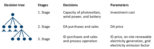
Figure 1: Structure of the integrated design and scheduling problem: The problem structure allows to optimize the design of the local electricity generation and storage system while considering simultaneous DA and ID market participation and process DR. The decision tree models the chronological sequence of the decisions. Each branch represents a scenario and each node represents a decision point.

Similar to our prior work (Germscheid et al.,, 2022), we consider hourly DA purchases and quarter-hourly ID purchases and sales and assume a one-day scheduling horizon. In addition, we allow to sell electricity from the local generation and storage system on the DA market. For simplicity, we assume that throughout any quarter-hour time slice, renewable electricity generation is constant.

In the following, we omit a distinct notation for second- and third-stage parameters and variables for better readability. In particular, we consider DA trading decisions $\bm{q}_{\text{DA,$s_{3}$}}$ and DA price $\bm{c}_{\text{DA,$s_{3}$}}$ on the third stage instead of the second stage and guarantee equality on the second stage by means of non-anticipativity constraints:

$$\bm{c}_{\text{DA,$s_{3}$}}=\bm{c}_{\text{DA},\hat{s}_{3}}\quad \text{if}\quad f(s_{3})=f(\hat{s}_{3})\quad\forall(s,\hat{s})\in\mathbb{S}_{3}\times\mathbb{S}_{3},$$ (1)

$$\bm{q}_{\text{DA,$s_{3}$}}=\bm{q}_{\text{DA},\hat{s}_{3}}\quad \text{if}\quad f(s_{3})=f(\hat{s}_{3})\quad\forall(s,\hat{s})\in\mathbb{S}_{3}\times\mathbb{S}_{3}$$ (2)

Here, $f:\mathbb{S}_{3}\xrightarrow{}\mathbb{S}_{2}$ maps a third-stage scenario $s_{3}\in\mathbb{S}_{3}$ to the respective second-stage scenario $s_{2}\in\mathbb{S}_{2}$. In the following, we refer to $s\in\mathbb{S}$ as third-stage scenario for conciseness. The non-anticipativity constraints allow to formulate the three-stage problem as a two-stage problem in the following.

2.2 Objectives

We consider the total annualized cost (TAC)and the global warming impact (GWI)as economic and ecologic objective, respectively.

The TAC is defined as

$$\text{\lx@glossaries@gls@link{acronym}{tac}{\leavevmode TAC}{}}=\text{CAPEX}+\text{OPEX}_{el}+\text{OPEX}_{Grid},$$ (3)

with $$\text{CAPEX}=\sum_{i\in\{\text{PV,W,B}\}}\left(\frac{(\gamma_{\text{1}}+1)^{\gamma_{2,i}}\gamma_{1}}{(\gamma_{1}+1)^{\gamma_{2,i}}-1}\text{CAPEX}^{0}_{i}\;Q_{i}+\gamma_{3,i}\;Q_{i}\right),$$ (4)

$$\text{OPEX}_{el}=365\sum_{s\in\mathbb{S}}\pi_{s}(4\;\Delta{t}\;{\bm{c}_{\text{DA,s}}}\cdot\bm{q}_{\text{DA,s}}+\Delta{t}\;\bm{c}_{\text{ID},s}\cdot\bm{q}_{\text{ID},s}),$$ (5)

$$\text{OPEX}_{\text{Grid}}=365\sum_{s\in\mathbb{S}}\pi_{s}\sum_{t=1}^{T}\text{OPEX}_{\text{Grid},s,t},$$ (6)

$$\text{OPEX}_{\text{Grid},s,t}\geq c_{\text{Fee}}\;\Delta{t}\;(q_{\text{DA,s,}\lfloor\frac{t-1}{4}\rfloor+1}+q_{\text{ID,}s,t}),$$ (7)

$$\text{OPEX}_{\text{Grid},s,t}\geq 0.$$ (8)

In Eq. 3, we compute the TAC as the sum of investment cost, CAPEX, and operational cost, OPEX. According to current legislation in Germany (Status 2023), the grid fee has to be paid in addition to the market price for electricity removed from the electricity grid (Bundesministerium der Justiz der Bundesrepublik Deutschland,, 2022). Thus, we consider both annual operational cost from electricity procurement, $\text{OPEX}_{el}$, as well as annual grid fee cost, $\text{OPEX}_{Grid}$. Eq. 4 specifies the investment cost of the local electricity generation and storage system considering photovoltaic (PV), wind power (W), and electric battery (B). Similar to Baumgärtner et al., (2019), we calculate the annualized CAPEX based on the total investment cost $\text{CAPEX}^{0}_{i}$, the present value factor with interest rate $\gamma_{1}$ and life time $\gamma_{2,i}$ (Broverman,, 2010), a maintenance factor $\gamma_{3,i}$, and the installed capacity of the respective technology $Q_{i}$. Note that in contrast to Baumgärtner et al., (2019), we consider a component-specific life time $\gamma_{2,i}$. Eq. 5 defines the electricity cost $\text{OPEX}_{el}$ by the purchases and sales on hourly DA and quarter-hourly ID electricity market $\bm{q}_{\text{DA,s}}$ and $\bm{q}_{\text{ID},s}$, the DA and ID electricity price $\bm{c}_{\text{DA,s}}$ and $\bm{c}_{\text{ID},s}$, the time step size $\Delta t=0.25$h, and the probability $\pi_{s}$ of scenario $s$. In Eq. 6, the grid cost $\text{OPEX}_{\text{Grid}}$ is derived from the sum of the grid cost $\text{OPEX}_{\text{Grid},s,t}$ of each scenario $s$ and time step $t$ with a total of 96 time steps for the one-day scheduling horizon, i.e, $T=96$. Eq. 7 and Eq. 8 constitute lower bounds for $\text{OPEX}_{\text{Grid},s,t}$, which ensure that $\text{OPEX}_{\text{Grid},s,t}$ is equal to zero in case of electricity injection into the grid and greater or equal to the grid fee with the grid fee cost $c_{\text{Fee}}$ in case of electricity removal from the grid. $\text{OPEX}_{\text{Grid},s,t}$ is equal to the respective lower limit, i.e., zero or the grid fee, when minimizing the TAC. Note that in $\text{OPEX}_{\text{Grid},s,t}$, $q_{\text{ID,}s,t}$ varies quarter-hourly and $q_{\text{DA,}s,t}$ varies hourly.

The expected annual GWI is computed as:

$$\text{\lx@glossaries@gls@link{acronym}{gwi}{\leavevmode GWI}{}}= 365\sum_{s\in\mathbb{S}}\pi_{s}\sum_{t=1}^{T}\Bigl{(}\text{GWI}^{\text{el}}_{s,t}\;\Delta{t}\;(q_{\text{DA,s,}\lfloor\frac{t-1}{4}\rfloor+1}+q_{\text{ID},s,t})\Bigl{)}+\sum_{i\in\{\text{PV,W,B}\}}\frac{\text{GWI}^{\text{i}}Q_{\text{i}}}{\gamma_{2,\text{i}}}$$ (9)

Eq. 9 considers the quarter-hourly average GWI of the electricity from the grid $\text{GWI}^{\text{el}}_{s,t}$, the GWI of the installed PV, wind power, and battery capacity, i.e., $\text{GWI}^{\text{PV}}$, $\text{GWI}^{\text{W}}$, and $\text{GWI}^{\text{B}}$, and their respective life time $\gamma_{2,i}$ in years. Consequently, the total annual GWI depends on hourly and quarter-hourly purchases and sales from the DA and ID market $q_{\text{DA,s,t}}$ and $q_{\text{ID,s,t}}$, respectively, and the installed PV, wind, and battery capacities, i.e., $\text{Q}^{\text{PV}}$, $\text{Q}^{\text{W}}$, and $\text{Q}^{\text{B}}$, respectively. Note that we allow for a GWI credit, i.e., negative GWI, in case of electricity sales accounting for an avoided emission burden (Horne et al.,, 2009).

2.3 Operational constraints

In the following, we shortly describe the generalized process model from our prior work (Schäfer et al.,, 2020; Germscheid et al.,, 2022) and discuss the operational constraints specific to the local energy system and the electricity trading.

The generalized process model (Schäfer et al.,, 2020) relies on few key parameters to describe the DR capabilities. In this work, we consider the key characteristics oversizing, minimal part load, product storage capacity with cyclic storage constraints, and ramping limitation. Note that without efficiency losses, the production rate of the process scales directly with the process power intake. For a detailed explanation of the generalized process model including the model equations, we refer to Germscheid et al., (2022).

In the electricity generation and storage system, we consider the DA and ID purchases and sales $q_{\text{DA,s,t}}$ and $q_{\text{ID,s,t}}$, respectively, with positive values corresponding to purchases. In addition, we consider PV power $q_{\text{PV,}s,t}$, wind power $q_{\text{W,}s,t}$, and battery charge and discharge $q_{\text{in,}s,t}$ and $q_{\text{out,}s,t}$ that together equate to the power intake $p_{s,t}$ of the production process by the energy balance:

$$p_{s,t} =q_{\text{DA,s,}\lfloor\frac{t-1}{4}\rfloor+1}+q_{\text{ID,}s,t}+q_{\text{PV,}s,t}+q_{\text{W,}s,t}-q_{\text{in,}s,t}+q_{\text{out,}s,t}$$ (10)

Additionally, we consider operational constraints similar to Baumgärtner et al., (2019):

$$q_{\text{PV,}s,t} =\bar{q}_{\text{PV,}s,t}\;Q_{\text{PV}},$$ (11)

$$q_{\text{W,}s,t} =\bar{q}_{\text{W,}s,t}\;Q_{\text{W}},$$ (12)

$$0 \leq q_{\text{in,}s,t}\leq Q_{\text{B}}/\tau,$$ (13)

$$0 \leq q_{\text{out,}s,t}\leq Q_{\text{B}}/\tau,$$ (14)

$$0 \leq SOC_{s,t}\leq Q_{\text{B}},$$ (15)

$$SOC_{s,t+1} =SOC_{s,t}+(\eta^{\text{in}}q_{\text{in,}s,t}-\frac{q_{\text{out,}s,t}}{\eta^{\text{out}}})\Delta{t},$$ (16)

$$SOC_{s,1} =SOC_{s,T+1}$$ (17)

Here, Eq. 11 and Eq. 12 define the PV and wind power generation, $q_{\text{PV,}s,t}$ and $q_{\text{W,}s,t}$, by multiplying the relative power output, $\bar{q}_{\text{PV,}s,t}$ and $\bar{q}_{\text{W,}s,t}$, with the installed PV and wind capacity, $Q_{\text{PV}}$ and $Q_{\text{W}}$, respectively. Eq. 13 and Eq. 14 constrain the battery charge and discharge, i.e., $q_{\text{in,}s,t}$ and $q_{\text{out,}s,t}$, respectively, by the installed battery capacity $Q_{\text{B}}$ and the allowed charging and discharging rate $\tau$. Eq. 15 constrains the state of charge $SOC_{s,t}$ by the installed battery capacity $Q_{\text{B}}$. Eq. 16 relates charging and discharging with respective efficiency losses $\eta^{\text{in}}$ and $\eta^{\text{out}}$ and the state of charge. Additionally, we consider the cyclic constraint, Eq. 17, requiring that the state of charge is the same at the beginning and at the end of the scheduling horizon.

We consider trading electricity on both DA and ID market while making use of the local energy system:

$$-q_{\text{PV,}s,t}-q_{\text{W,}s,t}-Q_{\text{B}}/\tau \leq q_{\text{DA,s,}\lfloor\frac{t-1}{4}\rfloor+1},$$ (18)

$$-q_{\text{PV,}s,t}-q_{\text{W,}s,t}-SOC_{s,t}/\Delta{t} \leq q_{\text{DA,s,}\lfloor\frac{t-1}{4}\rfloor+1},$$ (19)

$$-q_{\text{DA,s,}\lfloor\frac{t-1}{4}\rfloor+1}-q_{\text{PV,}s,t}-q_{\text{W,}s,t}-Q_{\text{B}}/\tau \leq q_{\text{ID},s,t},$$ (20)

$$-q_{\text{DA,s,}\lfloor\frac{t-1}{4}\rfloor+1}-q_{\text{PV,}s,t}-q_{\text{W,}s,t}-SOC_{s,t}/\Delta{t} \leq q_{\text{ID},s,t},$$ (21)

$$q_{\text{DA,s,}\lfloor\frac{t-1}{4}\rfloor+1} \leq P_{\text{nom}}(1+\theta_{\text{max}})+Q_{\text{B}}/\tau,$$ (22)

$$q_{\text{DA,s,}\lfloor\frac{t-1}{4}\rfloor+1} \leq P_{\text{nom}}(1+\theta_{\text{max}})+\frac{Q_{\text{B}}-SOC_{s,t}}{\Delta{t}},$$ (23)

$$q_{\text{ID},s,t} \leq P_{\text{nom}}(1+\theta_{\text{max}})+Q_{\text{B}}/\tau,$$ (24)

$$q_{\text{ID},s,t} \leq P_{\text{nom}}(1+\theta_{\text{max}})+\frac{Q_{\text{B}}-SOC_{s,t}}{\Delta{t}}$$ (25)

Here, Eqs. 18, 19, 20 and 21 constrain DA and ID sales by produced PV and wind power, the current state of charge, and maximum discharging capabilities of the installed battery. Similar to our prior work (Germscheid et al.,, 2022), Eqs. 20 and 21 allow to sell previously purchased DA electricity on the ID market. Eqs. 22, 23, 24 and 25 constrain DA and ID purchases by the maximum power consumption of the production process and the battery. The maximum consumption of the process is defined by the nominal consumption $P_{\text{nom}}$ and the process oversizing $\theta_{\text{max}}$. The maximum consumption of the battery is given by the state of charge and the charging capabilities of the battery.

2.4 Scenarios

We base our scenarios for the electricity price, wind power generation, PV power generation, and grid emission factor on historical time series. Specifically, for the electricity price, we use data from the German DA and ID spot market (Fraunhofer Institute for Solar Energy Systems ISE,, 2023), assuming that the consumer can purchase and sell electricity at DA market-clearing price and ID index price. We refer to Germscheid et al., (2022) for a detailed explanation about these assumptions. Fig. 2 shows the annual mean and the annual mean daily standard deviation of the ID electricity market price and the market deviation, i.e., the difference between the DA and the ID price. The corresponding figure for the DA price shows similar characteristics as the one of the ID price and can be found in Section 1 of the supporting material. Fig. 2(a) reveals a price decrease in 2020 that can be attributed to the initial phase of the COVID-19 pandemic (Halbrügge et al.,, 2021) and an increase of mean and standard deviation in 2021 and 2022 due to the conflict in the Ukraine (Haucap and Meinhof,, 2022). Fig. 2(b) reveals that in 2020 and 2021 the mean ID price was slightly larger than the mean DA price as indicated by the positive market deviation. Moreover, the standard deviation of the market deviation has significantly increased in 2021 and 2022. Note that DR scheduling optimization necessitates electricity price time series rather than an average annual electricity price. In our analysis, we pragmatically consider the time series of the years 2020, 2021, and 2022, assuming that these represent scenarios for low, medium, and high future electricity prices.

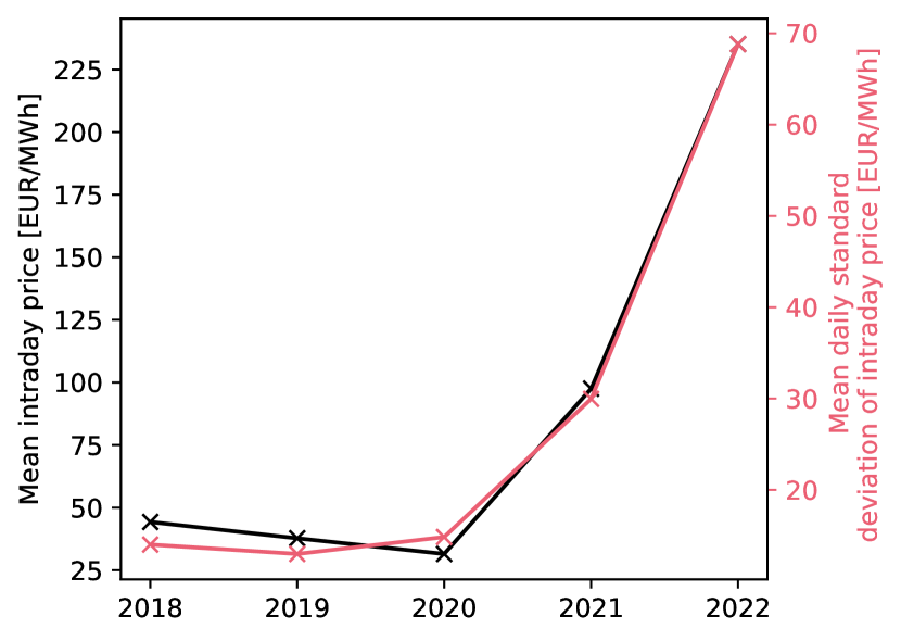
(a) ID electricity price

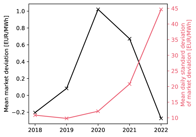
(b) Market deviation

Figure 2: Mean and mean daily standard deviation of ID electricity price (a) and market deviation (b), i.e., the price difference between the DA and the ID price.

To compute the corresponding historical wind and PV power time series, we use weather data for Aachen, Germany, from the German weather service (Deutscher Wetterdienst,, 2023; Gutzmann and Motl,, 2023). Specifically, we pre-process the measured wind speed, global radiation, and diffuse radiation similar to Bahl et al., (2017) and obtain the relative PV and wind power generation as discussed in detail in Section 2 of the supporting material. Section 1 of the supporting material shows the mean and the standard deviation of the historical weather data, from which it can be seen that mean and standard deviation of wind speed and solar irradiance stay within rather narrow ranges, with 2020 as a windier year and 2022 as a sunnier year.

Following Baumgärtner et al., (2019) and Nilges et al., (2023), we determine the average emission factor of electricity from the German grid for every time step, i.e., $\text{GWI}^{\text{el}}_{s,t}$ used in Eq. 9, by considering the momentary mix of power sources and their respective emission factors based on data of Bundesnetzagentur|smard.de, (2023) and the ecoinvent database (Wernet et al.,, 2016), respectively.

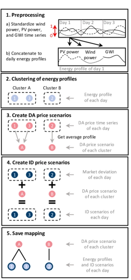
Figure 3: Approach to determine scenarios based on historical time series data: The colored dots refer to the multi-dimensional data points that represent (concatenated) time series data.

We determine the scenarios and the mapping between second and third stage of the optimization problem based on a clustering as depicted in Fig. 3. First, we preprocess the data by standardizing the wind and PV power time series and the GWI time series using the z-score (Mohamad and Usman,, 2013) and concatenating the daily profiles of wind power, PV power, and GWI time series to daily energy profiles. Next, we apply k-means clustering using the scikit-learn module in Python (Pedregosa et al.,, 2011) treating each daily energy profile as a multi-dimensional data point. This leads to a clustering of similar energy profiles. We transfer the obtained clustering to the DA price and market deviation time series and create an average DA profile as DA price scenario for each cluster. We add the market deviations from all constituents of a respective cluster to the average DA price scenario to obtain ID price scenarios. Note that using the market deviation allows to account for the inter-market correlation similar to our prior work (Germscheid et al.,, 2022). Finally, we use the mapping resulting from the clustering to connect the second and third stage of the optimization problem. Note that on the second stage, the probability of the DA scenarios depends on the cluster size. In contrast, the scenarios on the third stage are equi-probable, i.e., $\pi_{s}=1/|\mathbb{S}|$, as the clustering is used on the third stage for establishing the mapping but not for data reduction. We show in Section 3 of the supporting material that the within-cluster sum-of-squares does not allow to derive an obvious decision on a suitable number of clusters for the given data. For our application, we look for a compromise between the number of clusters and number of scenarios per cluster. Pragmatically, we consider 20 clusters, which leads to roughly 18 scenarios per cluster on average.

2.5 Model specifications and evaluation

We consider the parameters given in Tab. 1 for the CAPEX. Similar to Sass et al., (2020), we consider an interest rate $\gamma_{1}=8\%$. In Section 4 of the supporting material, we list the resulting annual PV and wind electricity generation cost showing that wind power has lower production cost than PV due to a higher average utilization rate. For the GWI of the electricity generation and storage system, we use data of the ecoinvent database 3.9.1 (Wernet et al.,, 2016) that we specify in Section 4 of the supporting material for reproducibility. For the battery, we consider a charging and discharging rate of 4h (Tesla,, 2023), i.e., $\tau=4$h, and a round-trip efficiency of $90\%$ (Hecking et al.,, 2018), i.e., $\sqrt{\eta_{\text{in}}}=\sqrt{\eta_{\text{out}}}=\sqrt{0.9}$. Moreover, we consider the average grid fee cost of 2022 for industrial consumers in Germany, i.e., $c_{\text{Fee}}=29.6$ EUR/MWh (Bundesnetzagentur und Bundeskartellamt,, 2022). Tab. 2 lists reference parameters of the generalized process that we also used in our prior work (Germscheid et al.,, 2022). Furthermore, we choose the nominal capacity such that the power-intensive production process is classified as an industrial consumer, i.e., 24 GWh per year (Bundesnetzagentur und Bundeskartellamt,, 2022), which allows the process operator to benefit from lower grid fees compared to non-industrial consumers (Bundesnetzagentur und Bundeskartellamt,, 2022).

Table 1: Component-specific life time, investment and maintenance cost for Germany based on Hecking et al., (2018).

	Lifetime $\gamma_{2,i}$	$\text{CAPEX}^{0}_{i}$	Annual maintenance cost $\gamma_{\text{2,i}}$
Roof-top PV	25 a	927 EUR/kWp	17 EUR/kWp
Onshore wind	25 a	1113 EUR/kWp	13 EUR/kWp
Battery	15 a	550 EUR/kWh	20 EUR/kWh

Table 2: Parameters of the generalized process model: Process oversizing, minimal part load, and ramping limit are given related to the nominal power intake. The product storage capacity refers to the time necessary to fill an empty product storage considering production at nominal power intake.

Parameter	Reference values
Nominal power intake	2.74 MW
Process oversizing	20%
Minimal part load	50%
Product storage capacity	3h
Ramping limit	25%/h

We expect the maximum allowed capacities of the energy system to have an impact on the optimization results. Pragmatically, we first restrict the admissible capacities for wind power and PV by the nominal power intake, i.e., $Q_{\text{W}}^{\text{max}}=Q_{\text{PV}}^{\text{max}}=P_{\text{nom}}$ and choose the admissible battery size such that the maximum discharge rate corresponds to the nominal power intake of the production process, i.e., $P_{\text{nom}}=Q_{\text{B}}^{\text{max}}/\tau$. In Section 3.2, we then analyze the impact of the maximum allowed energy system capacities on the TAC in detail.

We implement the model in Pyomo (Hart et al.,, 2011) and use the solver Gurobi 9.5.0 (Gurobi Optimization, LLC,, 2020) with default settings on an Intel Core i7-9700 processor and 32GB RAM. We formulate the multi-stage problem by means of its deterministic equivalent.

3 Results

In the following, we analyze the synergies between the local energy system and the flexible production process and the benefit of considering simultaneous market participation at design stage. To this end, we first consider market participation only on the ID market and discuss the optimal design and savings of the local energy system (Section 3.1) as well as the impact of the process flexibility on the potential savings (Section 3.2). Note that we select the ID market instead of the DA market, as the ID market allows to adapt the electricity procurement in response to realization of the uncertainty in the renewable electricity supply. We then show the difference between single and simultaneous market participation and discuss the energy system design in the context of DR scheduling with simultaneous DA and ID market participation (Section 3.3).

3.1 Design and operation for single market participation

In the following, we evaluate the energy system design considering only the ID market for the reference process defined in Tab. 2.

Fig. 4 shows Pareto-optimal energy system designs based on the time series for 2020, 2021, and 2022. For all three cases, the ecologic and economic objectives lead to competing solutions. Interestingly, the TAC-optimal solutions do not contain a battery, as potential savings from operating the battery do not outweigh the battery investment cost. High electricity prices in 2021 and 2022 incentivize both on-site wind and PV electricity generation in the TAC-optimal solutions, whereas only wind electricity generation is used in 2020. The preference for wind can be explained by the higher average utilization rate (see Section 4 of the supporting material). In contrast, battery, PV, and wind generation capacities are built at maximum capacity for all GWI-optimal solutions, irrespective of the year studied. The integration of a battery, however, leads to a large increase in TAC with only a small improvement in GWI, as can be seen from the shape of the Pareto front.

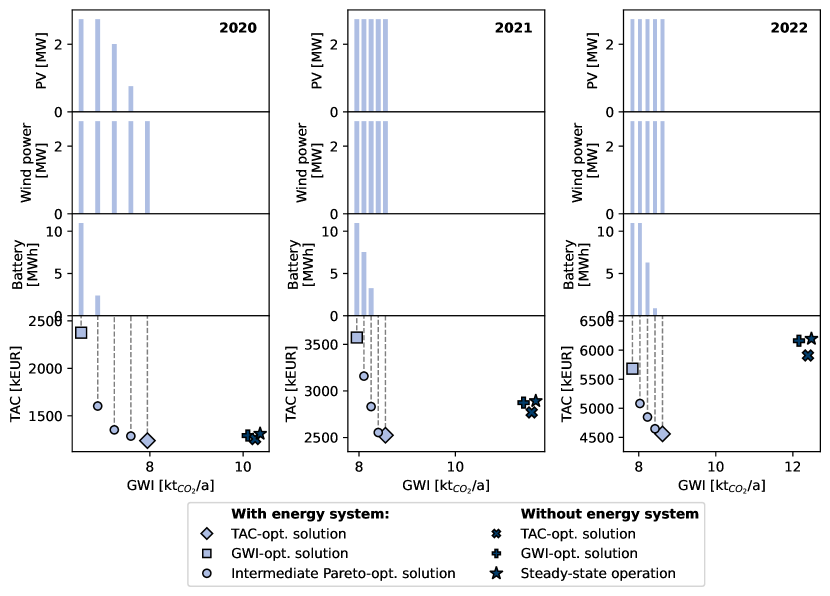
Figure 4: Energy system design for ID market-only participation: Pareto-optimal solutions are given for 2020 (left), 2021 (center), and 2022 (right). For each year, the TAC-optimal, the GWI-optimal, and three intermediate Pareto-optimal solutions are shown, which are equi-distant with respect to GWI. GWI and TAC (lower part) are given with vertical gray dashed lines pointing to the respective optimal capacities of the local electricity supply system (upper three parts). Additionally, the TAC- and GWI-optimal DR as well as the steady-state operation without a local energy system are given for comparison.

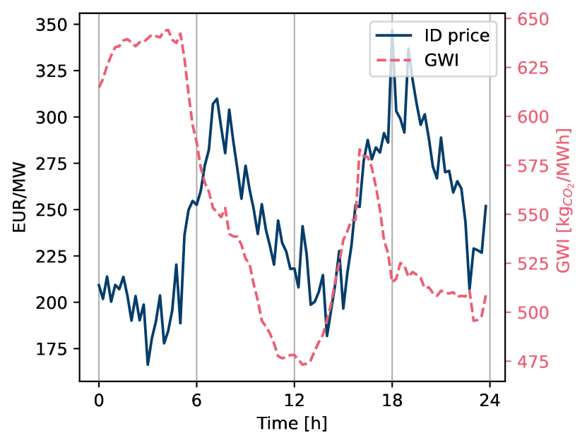
(a) Electricity price and emission factor.

(b) Renewable electricity generation.

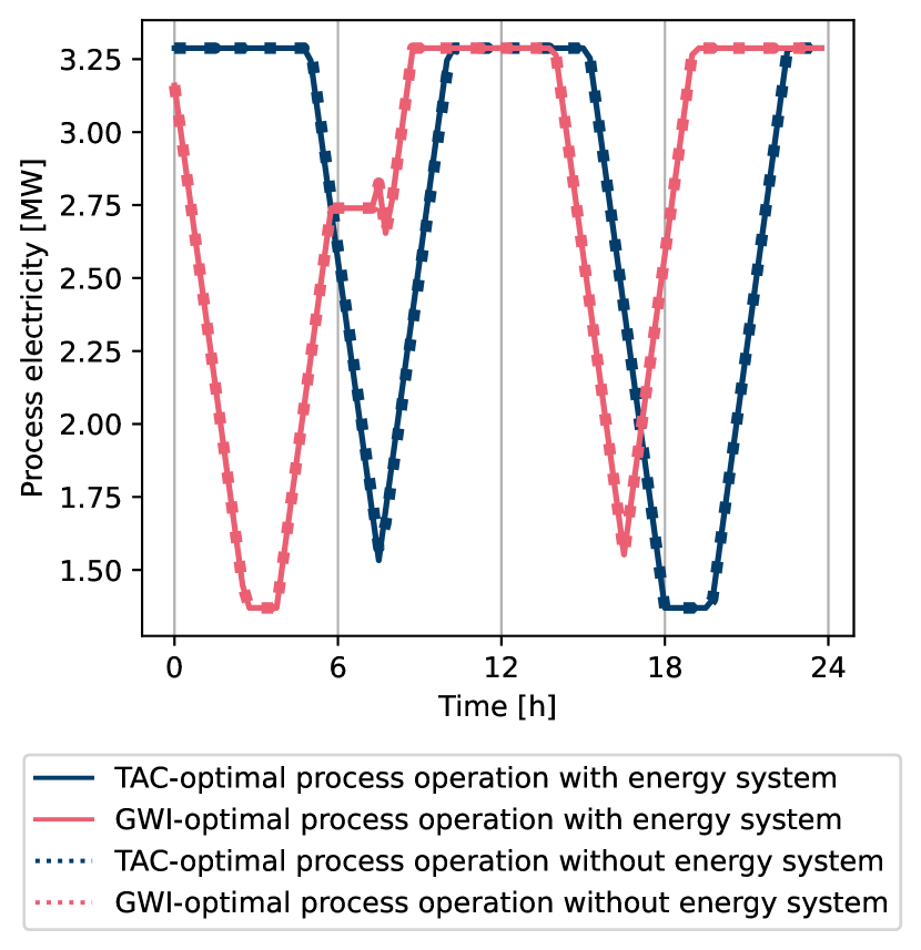
(c) Operation of the flexible reference process.

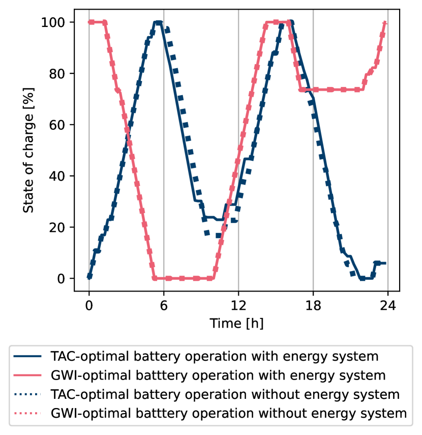
(d) Battery operation.

Figure 5: Process and energy system operation for an exemplary day in 2022 (ID-only market participation): An energy system design with maximum admissible PV, wind power, and battery capacities is considered. The operation is shown for the ID electricity price and emission factor (a) and the renewable electricity generation (b). The process operation determines the electricity consumption (c). The battery operation determines the state of charge (d).

Fig. 4 reveals that for 2022, the two designs with the lowest GWI have identical PV, wind power, and battery capacities but have notable differences in TAC and GWI, indicating different operating strategies. Fig. 5 shows the operation for an exemplary day given a fixed energy system design and confirms these findings. In particular, the electricity price and grid emission factor (Fig. 5(a)) set different incentives for TAC-optimal and GWI-optimal operation of the process (Fig. 5(c)) and the battery (Fig. 5(d)). Fig. 5(c) additionally shows the process operation without a local energy system, revealing a similar DR schedule as for a process with a local system. Similarly, Fig. 5(d) shows the battery operation with and without local renewable electricity generation revealing a similar operating pattern with only minor differences. We attribute this behavior to the time-varying incentives for DR at the operational level, i.e., the electricity price and the grid emission factor. The incentives predominantly influence the operation of the process and the local energy system, while on-site generated electricity has a minor influence.

Fig. 4 suggests that the difference between steady-state operation and DR without local energy system remains rather similar. In contrast, the difference between DR without energy system and DR with a local energy system has been increasing each year in particular with respect to the TAC. Tab. 3 compares ecologic and economic savings due to DR and the local energy system and confirms these findings. The absolute economic savings from DR in comparison to steady-state operation have been increasing due to the increasing standard deviation of the electricity price (Fig. 2(a)). The relative and absolute economic savings resulting from the energy system have been increasing due to the increasing grid electricity cost. In particular, the savings increased significantly from 1.4% in 2020 to 22.8% in 2022. Looking at the GWI-optimal solution, the ecologic savings resulting from the energy system are much larger than the savings from DR in comparison to steady-state operation. Furthermore, the ecologic savings are somewhat similar in all years, i.e., between 30.3% and 35.6%, and the variance can be attributed to the natural variability of PV and wind power production and the varying grid emission factor.

Table 3: Economic and ecologic savings due to DR and local electricity generation and storage. The savings are compared for the TAC-optimal solutions (upper part) and the GWI-optimal solutions (lower part). Single market participation on the ID market is considered.

	2020	2021	2022
TAC-optimal solution
DR vs steady-state operation (no energy system)
Relative economic savings	4.3%	4.2%	4.6%
Absolute economic savings [kEUR]	56	123	288
DR with energy system vs DR without energy system
Relative economic savings	1.4%	8.8%	22.8%
Absolute economic savings [kEUR]	17	245	1349
GWI-optimal solution
DR vs steady-state operation (no energy system)
Relative ecologic savings	2.5%	2.2%	2.6%
Absolute ecologic savings [kt${}_{{CO}_{2}}$/a]	0.3	0.3	0.3
DR with energy system vs DR without energy system
Relative ecologic savings	35.4%	30.3%	35.6%
Absolute ecologic savings [kt${}_{{CO}_{2}}$/a]	3.6	3.5	4.3

3.2 Parameter study of process flexibility and energy system capacity

In the following, we analyze which impact the process flexibility and admissible energy system capacities have on TAC and GWI.

For a parameter study on the process flexibility, we fix all process parameters to their respective reference values as defined in Tab. 2 and vary one process parameter at a time between the value corresponding to an inflexible process and the value corresponding to twice the flexibility of the process parameter. Fig. 6 shows the impact of varying degrees of process flexibility on the TAC-optimal DR without a local energy system, the economic savings enabled by a local energy system, and the optimal capacities for local electricity generation and storage. Fig. 6(a) (top) shows exemplary for 2020 that without a local energy system, the flexible process particularly benefits from oversizing. Behaviors for 2021 and 2022 are similar and thus the corresponding figures are omitted. The results confirm the findings of our prior work (Germscheid et al.,, 2022), where we considered price data of 2019. Furthermore, Fig. 6(a) (bottom) shows the optimal capacities of the energy system components and reveals that the optimal wind capacity for 2020 slightly decreases with a high degree of process oversizing, showing that the process flexibility can impact the optimal energy system capacity. Corresponding figures for 2021 and 2022 are omitted, as no impact of the process flexibility on the resulting optimal designs can be found.

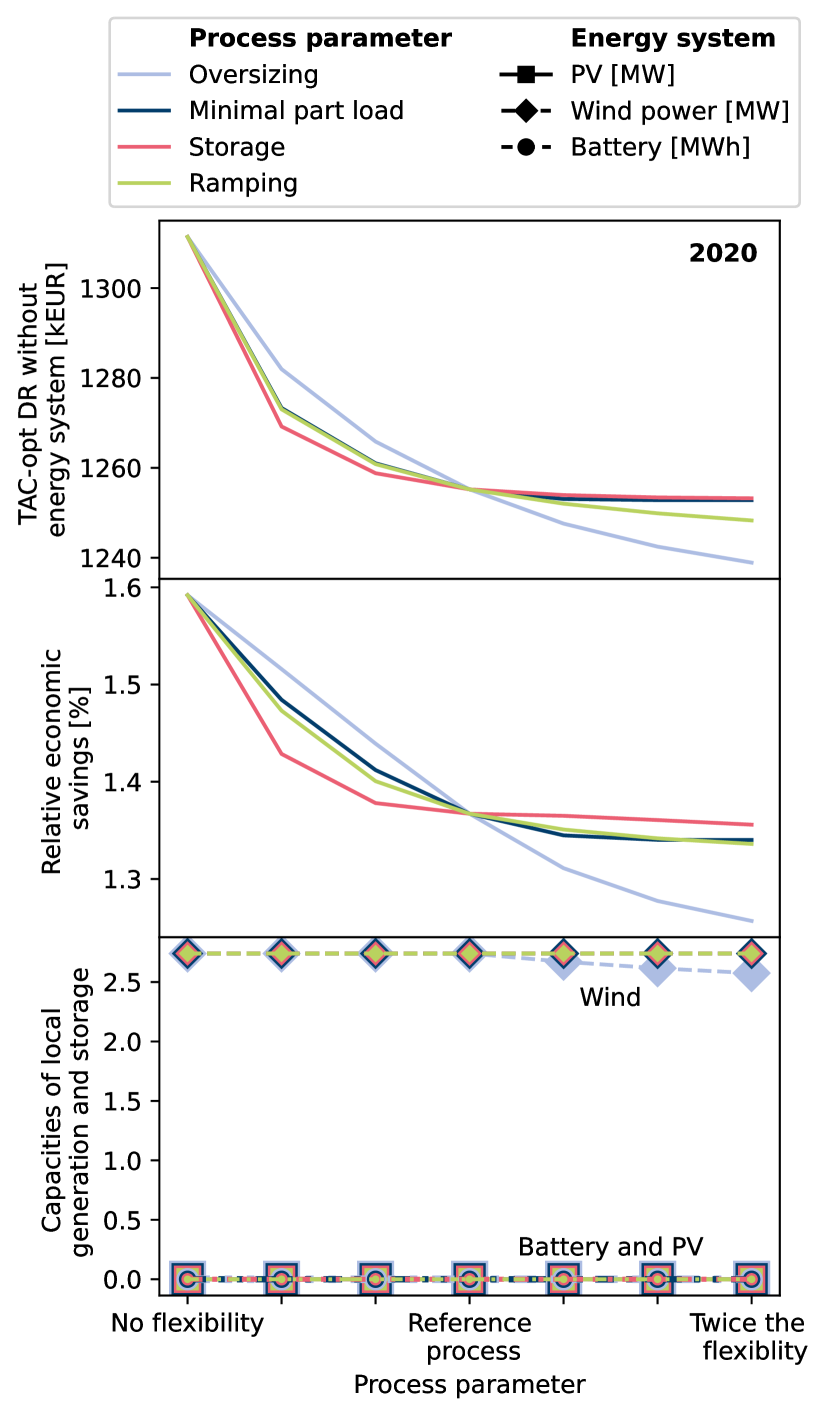
(a) TAC-optimal solutions for 2020.

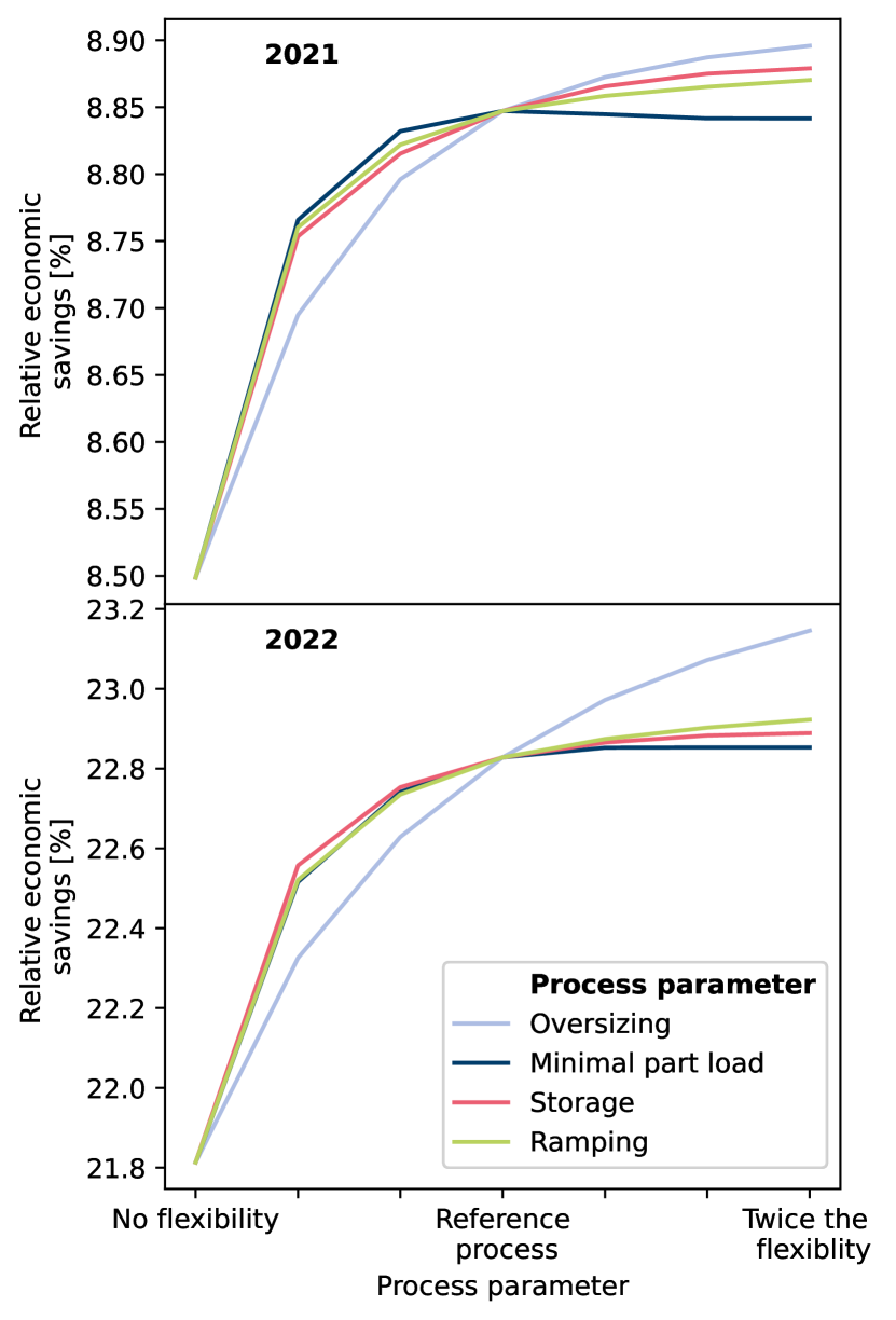
(b) Relative economic savings due to a local energy system for 2021 and 2022

Figure 6: Economic impact of different degrees of process flexibility: The TAC-optimal cost of DR without energy system (a, top), the savings due to a local energy system (a, center), and optimal energy system design (a, bottom) for 2020 are shown. Furthermore, the savings due to a local energy system are shown for 2021 (b, top) and 2022 (b, bottom).

Fig. 6 reveals that the range of the economic savings due to a local energy system for any given year is rather narrow, i.e., varying the process flexibility does not impact the relative savings in a strong manner. Varying the process oversizing has the largest leverage on the savings. Interestingly, the impact of the process parameters may differ depending on the investigated year, as higher process flexibility actually leads to lower relative savings in 2020 (Fig. 6(a), center) whereas higher relative savings are recorded for 2021 and 2022 (Fig. 6(b)). However, an analysis of the cost contributions shows exemplary for varying oversizing that the absolute TAC monotonously decreases, irrespective of the case with or without a local energy system (see Section 5 of the supporting material).

Fig. 7 shows the optimal TAC for varying admissible energy system size and process oversizing, the latter being the largest flexibility leverage for the economic savings. Specifically, we vary the maximum allowed energy system capacities, i.e., $Q_{\text{W}}^{\text{max}}$, $Q_{\text{PV}}^{\text{max}}$, and $Q_{\text{B}}^{\text{max}}$, by a joint scaling factor. Corresponding optimal capacities of the energy system can be found in Section 5 of the supporting material. For 2020, process oversizing has a larger leverage on the TAC than local electricity generation and storage. Furthermore, the TAC remains constant for scaling factors larger than one, as a cost-optimal maximum of the wind power capacity is attained (see Section 5 of the supporting material). For 2021 and 2022, it can be seen that local electricity generation and storage is more economically attractive than process flexibility.

Interestingly, the absolute savings of the TAC-optimal solution enabled by a higher process flexibility and by a larger energy system behave roughly additive, which is shown exemplary for 2022 in Fig. 7. Section 5 of the supporting material shows the relative difference between the optimal TAC and the estimated TAC, the latter being defined as the sum of the absolute savings from process flexiblization and installation of a local energy system. The difference being rather small, i.e., less than 0.5%, means that a quick first approximate economic assessment can be performed by considering the savings from DR and the cost savings from a local energy system independently.

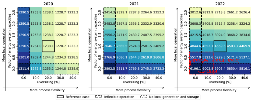
Figure 7: Optimal TAC [EUR] with varying process oversizing and maximum admissible energy system capacity for 2020 (left), 2021 (center), and 2022 (right): For 2022, the approximately additive behavior of the absolute savings is shown exemplary in red.

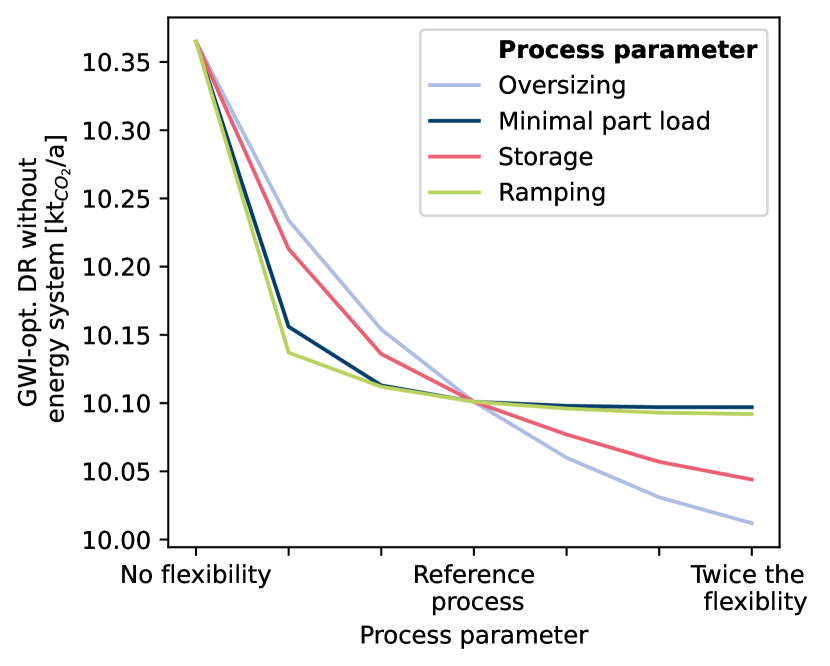
(a) GWI-optimal DR without a local energy system

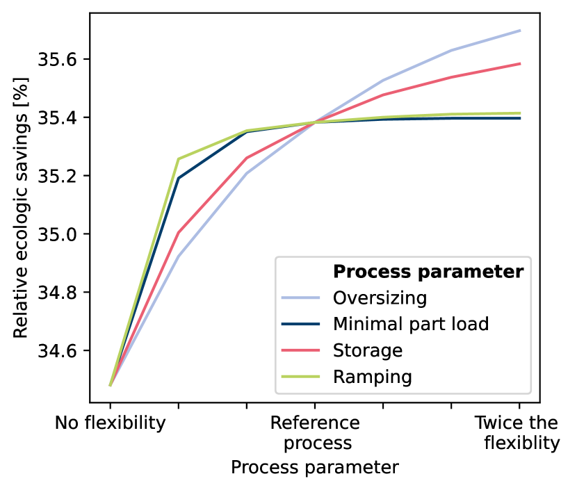
(b) Relative ecologic savings due to a local energy system

Figure 8: Ecologic impact of varying process flexibility for 2020: GWI-optimal DR without a local energy system (a) and relative savings due to installation of a local system (b) are shown.

Fig. 8 shows the impact of varying degrees of process flexibility on the GWI-optimal solution exemplary for 2020. Figures for the other years show similar behavior and are therefore omitted. Fig. 8(a) shows the case of DR without a local energy system and reveals that the process oversizing and the product storage capacity have the largest impact on the GWI. This finding is consistent with the results of our prior work (Schäfer et al.,, 2020), where we considered the residual load as ecologic objective instead of the GWI. Fig. 8(b) shows that process oversizing and product storage capacity have the largest leverage on the ecologic savings. Note that, in general, the degree of process flexibility has a rather low impact on the range of the ecologic savings.

3.3 Simultaneous market participation

Finally, we evaluate the benefit of considering simultaneous DA and ID market participation in the integrated design and scheduling problem. Tab. 4 lists the TAC-optimal designs for the reference process. Designs for 2020 and 2021 do not reveal differences to the case of ID-only market participation, i.e., the price differences between the markets in these years are not large enough to incentivize the installation of a battery. In contrast, a battery is built for the simultaneous market participation in 2022 as the battery offers trading capacity for exploitation of large price differences between the DA and ID market. The Pareto-optimal energy system designs of 2022 vary with respect to the battery capacity for the simultaneous DA and ID market participation compared to the ID-only case and are shown in Section 6 of the supporting material.

Table 4: System capacities and electricity trading amounts for ID-only participation (upper part) and simultaneous DA and ID market participation (lower part): In all cases, TAC-optimal DR of the reference process (Tab. 2) with a local energy system is considered. The stated values of the ID-only participation correspond to the TAC-optimal solution from Fig. 4.

	2020	2021	2022
ID-only participation
PV capacity	-	2.74 MW	2.74 MW
Wind capacity	2.74 MW	2.74 MW	2.74 MW
Battery capacity	-	-	-
Total purchases	17,316 MWh	16,008 MWh	14,776 MWh
Total sales	62 MWh	203 MWh	357 MWh
Simultanous market participation
PV capacity	-	2.74 MW	2.74 MW
Wind capacity	2.74 MW	2.74 MW	2.74 MW
Battery capacity	-	-	5.31 MWh
DA purchases	18,582 MWh	16,389 MWh	18,874 MWh
ID purchases	6,796 MWh	7,442 MWh	12,944 MWh
Total purchases	25,378 MWh	23,831 MWh	31,818 MWh
DA sales	452 MWh	954 MWh	5,947 MWh
ID sales	7,678 MWh	7,080 MWh	11,083 MWh
Total sales	8,130 MWh	8,034 MWh	17,030 MWh

Tab. 4 compares single and simultaneous market participation with respect to the electricity purchases and sales. It shows that for ID-only participation more electricity is purchased in 2020, compared to 2021 and 2022, which are years with larger optimal PV and wind power capacities. For the simultaneous participation in 2020, the majority of the electricity is purchased on the DA market due the positive price difference (Fig. 2(b)). The combination of PV and wind enables higher DA sales in 2021. Moreover, total purchases and sales significantly increase for the simultaneous participation in 2022 due to an increased trading capacity enabled by the battery.

Tab. 5 shows that the relative savings of simultaneous market participation compared to single market participation stay within a similar range, irrespective of the considered year. In contrast, the absolute savings have been increasing each year due to the increased variance of the market deviation (Fig. 2(b)). Tab. 5 reveals that both the absolute and relative savings of simultaneous market participation increase with both process flexibilization and the integration of local electricity generation and storage.

Table 5: The TAC savings from simultaneous market participation compared to single market participation for an inflexible process without an energy system (top), a flexible process without an energy system (center), and a flexible process with an energy system (bottom). The flexible process is the reference process (Tab. 2).

	2020	2021	2022
Inflexible process without energy system
Relative savings	3.0%	2.0%	2.0%
Absolute savings	39.3 kEUR	57.4 kEUR	122.7 kEUR
Flexible process without energy system
Relative savings	3.8%	2.5%	2.5%
Absolute savings	47.1 kEUR	68.9 kEUR	147.2 kEUR
Flexible process with energy system
Relative savings	3.9%	2.9%	4.4%
Absolute savings	47.9 kEUR	72.8 kEUR	198.7 kEUR

Tab. 6 shows the contributions of cost savings for the year 2022 considering TAC-optimal simultaneous market participation. Here, an inflexible process without an energy system is modified by adding a battery, renewable electricity generation, and process flexiblization, separately. Tab. 6 reveals that the main cost savings result from the on-site electricity generation followed by process flexiblization. The integration of a battery accounts only for a small fraction of the savings. Note that similar to ID-only participation (Section 3.2), summing up the absolute savings from battery installation, renewable electricity generation, and flexiblization, separately, allows for a good overall savings estimate.

Table 6: Savings contributions of simultaneous market participation in the TAC-optimal case for 2022: The savings are related to the inflexible process without an energy system (first row). The battery capacity of the inflexible process with the battery (third row) is identical to the flexible process with an energy system (second row).

	TAC	Savings
Inflexible process without energy system	6073.5 kEUR	-
Flexible process with energy system	4360.9 kEUR	1712.6 kEUR
Inflexible process with battery	6044.7 kEUR	28.8 kEUR
Inflexible process with wind and PV power	4702.5 kEUR	1371.0 kEUR
Flexible process without energy system	5761.2 kEUR	312.3 kEUR

Finally, similar to Section 3.2, we vary the degree of process flexibility. Fig. 9 shows the impact of process flexibility on the optimal battery capacity for 2022. An analysis of the optimal capacities of PV and wind power is omitted as these quantities do not vary in response to a varying degree of process flexibility. It can be noted that larger batteries are built for less flexible processes, in particular for processes with part load and ramping restrictions. DR without energy system and economic savings of DR with an energy system behave similar to the case of single market participation (Section 3.2), irrespective of the investigated year. Thus, respective figures are omitted.

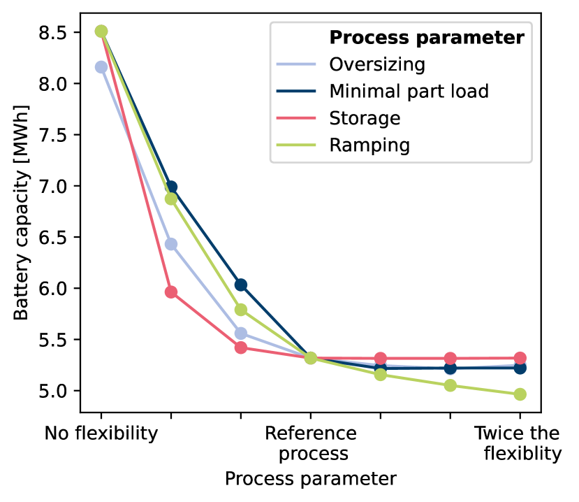
Figure 9: TAC-optimal battery capacity for simultaneous market participation for 2022 with varying degree of process flexibility.

4 Conclusion

We assessed the optimal design of a local electricity generation and storage system for a generalized continuous, power-intensive production process that is capable of performing demand response and can act on both the day-ahead and intraday electricity market. In a three-stage stochastic problem, we optimized the capacities of photovoltaic power, wind power, and electric battery with an integrated demand response scheduling of the production process. Building on our prior work (Schäfer et al.,, 2020; Germscheid et al.,, 2022), we used a generalized process model with few flexibility-defining parameters, i.e., process oversizing, minimal part load, product storage, and ramping limitation. In a bi-objective optimization, we considered both economic and ecologic objectives. We considered scenarios of low, intermediate, and high electricity prices for a plant location in Germany as well as a time-varying grid emission factor.

We find that batteries are mainly built to lower the global warming impact, however, leading to a significant increase in total annualized cost. Economic and ecologic process and battery operation primarily respond to the time-varying electricity price and grid emission factor, but only to a little extent to the on-site generation of renewable electricity. Varying the degree of process flexibility, we find a rather small impact on the achievable relative economic and ecologic savings that come with local electricity generation and storage. Moreover, we show that the absolute cost savings from flexiblizing the process and installing a local energy system are approximately additive. Comparing intraday-only and simultaneous day-ahead and intraday market participation, we find that the energy system designs are similar for the investigated scenarios, except when high price differences between the markets incentivize the installation of a battery. The cost-optimal battery capacity significantly depends on the available process flexibility, enables large volumes for trading on the markets, but comes with only minor economic savings.

In order to use our approach to evaluate the benefit of optimally sizing a local electricity generation and storage system for a specific process and location, the process characteristics must be known, respective local weather data is required, and electricity price scenarios have to be created. Considering the long lifetime of a process and the energy system equipment, long-term electricity price scenarios with measures of uncertainty and the associated financial risk should be accounted for, e.g., similar to Xuan et al., (2021); Vieira et al., (2021).

Authorship contribution

Sonja H. M. Germscheid: Conceptualization, Methodology, Software, Investigation, Data curation, Writing - original draft, Visualization. Benedikt Nilges: Data curation, Writing – review & editing. Niklas von der Assen: Funding acquisition, Writing – review & editing. Alexander Mitsos: Writing - review & editing, Supervision, Funding acquisition. Manuel Dahmen: Conceptualization, Methodology, Writing - review & editing, Supervision, Funding acquisition.

Declaration of Competing Interest

We have no conflict of interest.

References

- Allman and Daoutidis, (2018) Allman, A. and Daoutidis, P. (2018). Optimal scheduling for wind-powered ammonia generation: Effects of key design parameters. Chemical Engineering Research and Design, 131:5–15.
- Bahl et al., (2017) Bahl, B., Kümpel, A., Seele, H., Lampe, M., and Bardow, A. (2017). Time-series aggregation for synthesis problems by bounding error in the objective function. Energy, 135:900–912.
- Bahl et al., (2018) Bahl, B., Söhler, T., Hennen, M., and Bardow, A. (2018). Typical periods for two-stage synthesis by time-series aggregation with bounded error in objective function. Frontiers in Energy Research, 5(January):1–13.
- Baumgärtner et al., (2019) Baumgärtner, N., Delorme, R., Hennen, M., and Bardow, A. (2019). Design of low-carbon utility systems: Exploiting time-dependent grid emissions for climate-friendly demand-side management. Applied Energy, 247(April):755–765.
- Birge and Louveaux, (2011) Birge, J. R. and Louveaux, F. (2011). Introduction to Stochastic Programming. Springer Series in Operations Research and Financial Engineering. Springer New York, New York, NY.
- Broverman, (2010) Broverman, S. (2010). Mathematics of Investment and Credit. ACTEX Publications, Inc., 5 edition.
- Bundesministerium der Justiz der Bundesrepublik Deutschland, (2022) Bundesministerium der Justiz der Bundesrepublik Deutschland (2022). Stromnetzentgeltverordnung vom 25. Juli 2005 (BGBl. I S. 2225), die zuletzt durch Artikel 6 des Gesetzes vom 20. Juli 2022 (BGBl. I S. 1237) geändert worden ist. https://www.gesetze-im-internet.de/stromnev/BJNR222500005.html##BJNR222500005BJNG000500000 (accessed 12-09-2023).
- Bundesnetzagentur und Bundeskartellamt, (2022) Bundesnetzagentur und Bundeskartellamt (2022). Monitoringbericht 2020. https://www.bundesnetzagentur.de/DE/Fachthemen/ElektrizitaetundGas/Monitoringberichte/start.html (accessed 24-04-2023).
- Bundesnetzagentur|smard.de, (2023) Bundesnetzagentur|smard.de (2023). SMARD Strommarktdaten. https://www.smard.de/home (accessed 2023-10-10).
- Burre et al., (2020) Burre, J., Bongartz, D., Brée, L., Roh, K., and Mitsos, A. (2020). Power-to-X: Between Electricity Storage, e-Production, and Demand Side Management. Chemie Ingenieur Technik, 92(1-2):74–84.
- Dalle Ave et al., (2019) Dalle Ave, G., Harjunkoski, I., and Engell, S. (2019). A non-uniform grid approach for scheduling considering electricity load tracking and future load prediction. Computers & Chemical Engineering, 129:106506.
- Daryanian et al., (1989) Daryanian, B., Bohn, R. E., and Tabors, R. D. (1989). Optimal Demand-Side Response to Electricity Spot Prices for Storage-Type Customers. IEEE Power Engineering Review, 9(8):36–36.
- Deutscher Wetterdienst, (2023) Deutscher Wetterdienst (2023). Open Data. https://opendata.dwd.de/ (accessed 19-04-2023).
- Fleschutz et al., (2023) Fleschutz, M., Bohlayer, M., Braun, M., and Murphy, M. D. (2023). From prosumer to flexumer: Case study on the value of flexibility in decarbonizing the multi-energy system of a manufacturing company. Applied Energy, 347(January):121430.
- Fraunhofer Institute for Solar Energy Systems ISE, (2023) Fraunhofer Institute for Solar Energy Systems ISE (2023). Energy Charts. https://www.energy-charts.info (accessed 2023-08-06).
- Germscheid et al., (2023) Germscheid, S. H., Röben, F. T., Sun, H., Bardow, A., Mitsos, A., and Dahmen, M. (2023). Demand response scheduling of copper production under short-term electricity price uncertainty. Computers & Chemical Engineering, 178:108394.
- Germscheid et al., (2022) Germscheid, S. H. M., Mitsos, A., and Dahmen, M. (2022). Demand response potential of industrial processes considering uncertain short-term electricity prices. AIChE Journal, 68(11):e17828.
- Golmohamadi and Keypour, (2018) Golmohamadi, H. and Keypour, R. (2018). Stochastic optimization for retailers with distributed wind generation considering demand response. Journal of Modern Power Systems and Clean Energy, 6(4):733–748.
- Gurobi Optimization, LLC, (2020) Gurobi Optimization, LLC (2020). Gurobi optimizer reference manual. http://www.gurobi.com (accessed 01-06-2021).
- Gutzmann and Motl, (2023) Gutzmann, B. and Motl, A. (2023). Wetterdienst.
- Halbrügge et al., (2021) Halbrügge, S., Schott, P., Weibelzahl, M., Buhl, H. U., Fridgen, G., and Schöpf, M. (2021). How did the German and other European electricity systems react to the COVID-19 pandemic? Applied Energy, 285(November 2020):116370.
- Hart et al., (2011) Hart, W. E., Watson, J.-P., and Woodruff, D. L. (2011). Pyomo: modeling and solving mathematical programs in Python. Mathematical Programming Computation, 3(3):219–260.
- Haucap and Meinhof, (2022) Haucap, J. and Meinhof, J. (2022). Die Strompreise der Zukunft. Wirtschaftsdienst, 102(S1):53–60.
- Hecking et al., (2018) Hecking, H., Kruse, J., Hennes, O., Wildgrube, T., Lencz, D., Hintermayer, M., Gierkink, M., and Lorenczik, J. P. D. S. (2018). dena-Leitstudie Integrierte Energiewende. https://shop.dena.de/fileadmin/denashop/media/Downloads_Dateien/esd/9262_dena-Leitstudie_Integrierte_Energiewende_Ergebnisbericht.pdf (accessed 19-04-2023).
- Horne et al., (2009) Horne, R. E., Grant, T., and Verghese, K. (2009). Life Cycle Assessment : Principles, Practice and Prospects. Csiro Publishing, Collingwood, Australia.
- Kwon et al., (2017) Kwon, S., Ntaimo, L., and Gautam, N. (2017). Optimal Day-Ahead Power Procurement With Renewable Energy and Demand Response. IEEE Transactions on Power Systems, 32(5):3924–3933.
- Langiu et al., (2022) Langiu, M., Dahmen, M., and Mitsos, A. (2022). Simultaneous optimization of design and operation of an air-cooled geothermal ORC under consideration of multiple operating points. Computers & Chemical Engineering, 161:107745.
- Leenders et al., (2019) Leenders, L., Bahl, B., Lampe, M., Hennen, M., and Bardow, A. (2019). Optimal design of integrated batch production and utility systems. Computers & Chemical Engineering, 128:496–511.
- Leo et al., (2021) Leo, E., Dalle Ave, G., Harjunkoski, I., and Engell, S. (2021). Stochastic short-term integrated electricity procurement and production scheduling for a large consumer. Computers & Chemical Engineering, 145:107191.
- Liu et al., (2016) Liu, G., Xu, Y., and Tomsovic, K. (2016). Bidding Strategy for Microgrid in Day-Ahead Market Based on Hybrid Stochastic/Robust Optimization. IEEE Transactions on Smart Grid, 7(1):227–237.
- Martín, (2016) Martín, M. (2016). Methodology for solar and wind energy chemical storage facilities design under uncertainty: Methanol production from CO2 and hydrogen. Computers & Chemical Engineering, 92:43–54.
- Mitra et al., (2014) Mitra, S., Pinto, J. M., and Grossmann, I. E. (2014). Optimal multi-scale capacity planning for power-intensive continuous processes under time-sensitive electricity prices and demand uncertainty. Part I: Modeling. Computers & Chemical Engineering, 65:89–101.
- Mitsos et al., (2018) Mitsos, A., Asprion, N., Floudas, C. A., Bortz, M., Baldea, M., Bonvin, D., Caspari, A., and Schäfer, P. (2018). Challenges in process optimization for new feedstocks and energy sources. Computers & Chemical Engineering, 113:209–221.
- Mohamad and Usman, (2013) Mohamad, I. B. and Usman, D. (2013). Standardization and its effects on k-means clustering algorithm. Research Journal of Applied Sciences, Engineering and Technology, 6(17):3299–3303.
- Mucci et al., (2023) Mucci, S., Mitsos, A., and Bongartz, D. (2023). Cost-optimal Power-to-Methanol: Flexible operation or intermediate storage? Journal of Energy Storage, 72:108614.
- Nilges et al., (2023) Nilges, B., Burghardt, C., Roh, K., Reinert, C., and von der Aßen, N. (2023). Comparative life cycle assessment of industrial demand-side management via operational optimization. Computers & Chemical Engineering, 177(March):108323.
- Nolzen et al., (2022) Nolzen, N., Ganter, A., Baumgärtner, N., Leenders, L., and Bardow, A. (2022). Where to market flexibility? Optimal participation of industrial energy systems in balancing-power, day-ahead, and continuous intraday electricity markets.
- Pandžić et al., (2013) Pandžić, H., Morales, J. M., Conejo, A. J., and Kuzle, I. (2013). Offering model for a virtual power plant based on stochastic programming. Applied Energy, 105:282–292.
- Pedregosa et al., (2011) Pedregosa, F., Varoquaux, G., Gramfort, A., Michel, V., Thirion, B., Grisel, O., Blondel, M., Prettenhofer, P., Weiss, R., Dubourg, V., Vanderplas, J., Passos, A., Cournapeau, D., Brucher, M., Perrot, M., and Duchesnay, E. (2011). Scikit-learn: Machine learning in Python. Journal of Machine Learning Research, 12:2825–2830.
- Sass et al., (2020) Sass, S., Faulwasser, T., Hollermann, D. E., Kappatou, C. D., Sauer, D., Schütz, T., Shu, D. Y., Bardow, A., Gröll, L., Hagenmeyer, V., Müller, D., and Mitsos, A. (2020). Model compendium, data, and optimization benchmarks for sector-coupled energy systems. Computers & Chemical Engineering, 135:106760.
- Schäfer et al., (2020) Schäfer, P., Daun, T. M., and Mitsos, A. (2020). Do investments in flexibility enhance sustainability? A simulative study considering the German electricity sector. AIChE Journal, 66(11):1–14.
- Schäfer et al., (2019) Schäfer, P., Westerholt, H. G., Schweidtmann, A. M., Ilieva, S., and Mitsos, A. (2019). Model-based bidding strategies on the primary balancing market for energy-intense processes. Computers & Chemical Engineering, 120:4–14.
- Seo et al., (2023) Seo, K., Retnanto, A. P., Martorell, J. L., Edgar, T. F., Stadtherr, M. A., and Baldea, M. (2023). Simultaneous design and operational optimization for flexible carbon capture process using ionic liquids. Computers & Chemical Engineering, 178:108344.
- Simkoff and Baldea, (2020) Simkoff, J. M. and Baldea, M. (2020). Stochastic scheduling and control using data-driven nonlinear dynamic models: Application to demand response operation of a chlor-alkali plant. Industrial & Engineering Chemistry Research, 59(21):10031–10042.
- Steimel and Engell, (2015) Steimel, J. and Engell, S. (2015). Conceptual design and optimization of chemical processes under uncertainty by two-stage programming. Computers & Chemical Engineering, 81:200–217.
- Teichgraeber and Brandt, (2020) Teichgraeber, H. and Brandt, A. R. (2020). Optimal design of an electricity-intensive industrial facility subject to electricity price uncertainty: Stochastic optimization and scenario reduction. Chemical Engineering Research and Design, 163:204–216.
- Tesla, (2023) Tesla (2023). Product Details. https://www.tesla.com/megapack/design (accessed 2023-07-24).
- Varelmann et al., (2022) Varelmann, T., Erwes, N., Schäfer, P., and Mitsos, A. (2022). Simultaneously optimizing bidding strategy in pay-as-bid-markets and production scheduling. Computers & Chemical Engineering, 157:107610.
- Vieira et al., (2021) Vieira, M., Paulo, H., Pinto-Varela, T., and Barbosa-Póvoa, A. P. (2021). Assessment of financial risk in the design and scheduling of multipurpose plants under demand uncertainty. International Journal of Production Research, 59(20):6125–6145.
- Voll et al., (2013) Voll, P., Klaffke, C., Hennen, M., and Bardow, A. (2013). Automated superstructure-based synthesis and optimization of distributed energy supply systems. Energy, 50(1):374–388.
- Wang et al., (2020) Wang, G., Mitsos, A., and Marquardt, W. (2020). Renewable production of ammonia and nitric acid. AIChE Journal, 66(6):1–9.
- Wernet et al., (2016) Wernet, G., Bauer, C., Steubing, B., Reinhard, J., Moreno-Ruiz, E., and Weidema, B. (2016). The ecoinvent database version 3 (part I): Overview and methodology. The International Journal of Life Cycle Assessment, 21(9):1218–1230.
- Xuan et al., (2021) Xuan, A., Shen, X., Guo, Q., and Sun, H. (2021). A conditional value-at-risk based planning model for integrated energy system with energy storage and renewables. Applied Energy, 294(52007123):116971.
- Yunt et al., (2008) Yunt, M., Chachuat, B., Mitsos, A., and Barton, P. I. (2008). Designing man-portable power generation systems for varying power demand. AIChE Journal, 54(5):1254–1269.
- Zhang and Grossmann, (2016) Zhang, Q. and Grossmann, I. E. (2016). Planning and scheduling for industrial demand side management: Advances and challenges. In Alternative Energy Sources and Technologies, pages 383–414. Springer International Publishing.
- Zhang et al., (2019) Zhang, Q., Martín, M., and Grossmann, I. E. (2019). Integrated design and operation of renewables-based fuels and power production networks. Computers & Chemical Engineering, 122(2):80–92.