Microscopic theory of field tuned topological transitions in the Kitaev honeycomb model

Abstract

We microscopically derive an abelian mutual Chern-Simons lattice gauge theory for a honeycomb Kitaev model subjected to time reversal symmetry breaking $(001)$ Zeeman and three-body scalar spin chirality perturbations. We identify the nature of topological orders, emergent excitations and ground state degeneracy (GSD), topological entanglement entropy ($\gamma$), and chiral central charge ($c$) in different field regimes for both ferromagnetic (FM) and antiferromagnetic (AFM) sign of the Kitaev interaction. A nonabelian Ising topological order (ITO) exists at low fields in both cases, with $\gamma=\ln 2,$ $c=1/2,$ and GSD$=3,$ where the nonabelian anyon, a twist defect, is an intrinsic bulk excitation. For AFM Kitaev interactions, a topologically trivial phase with central charge $c=1/2$ appears at intermediate fields, thus implying half-quantized thermal Hall response in both low and intermediate field phases with no change of sign. At higher fields there is a final transition to a partially polarized paramagnetic phase with $\gamma=c=0.$ For the FM case, there is a direct transition from ITO to the polarized phase.

Study of topological orders and their stability against perturbations is a central topic of current interest in condensed matter physics [1, 2, 3, 4, 5, 6, 7, 8, 9, 10, 11, 12, 13]. In the gapless spin liquid phase of the honeycomb Kitaev model, time reversal symmetry breaking perturbations such as scalar spin chirality interactions result in Ising topological order (ITO) [12], while with increasing Zeeman perturbations, ITO is lost beyond a certain threshold field [14, 15, 16, 17, 18, 19]. However there are major gaps in our knowledge of the bulk excitations, topological degeneracy and entanglement entropy, and the chiral central charge $c$ of the edge theory except perhaps at the lowest fields. In the low field regime, recent perturbative treatments [20, 21] going beyond parton-based mean field theory emphasize the important role of vison (gauge field) fluctuation effects but these calculations are focused primarily on the chiral central charge and a full understanding of the nature of the finite field phases is still awaited. Numerical treatments get complicated by finite size effects making it difficult to obtain properties such as the topological degeneracy and entanglement entropy when correlation lengths are not sufficiently small [16, 19, 22]. Experimentally, Kitaev materials have even more complicated interactions, and there is great interest in the possibility of ITO revival near field-suppressed magnetic order [23, 24]. Such questions have also inspired phenomenological studies of topological phases and excitations in relevant matter Chern-Simons field theories [25, 26]. However before attempting a microscopic treatment of the intermediate field phases in Kitaev materials, it is important to first understand the behavior in the Kitaev limit.

We present here a microscopic derivation and analysis of an effective topological gauge theory using a Chern-Simons fermionization of the spins recently introduced by us [27] where the fermions are attached in specific ways to two distinct abelian $Z_{2}$ gauge fields respectively on the lattice and dual lattice. Such enlargement of the gauge degrees of freedom is necessary for satisfaction of the Chern-Simons Gauss-law constraints on arbitrary lattices generally lacking local one-to-one face-vertex correspondence [28, 29, 30, 31]. Our matter Chern-Simons theory requires conservation of fermion number parity, and we consider time-reversal symmetry breaking perturbations that are consistent with this condition. We construct the quasiparticles and obtain their fusion rules, together with topological ground state degeneracy (GSD), entanglement entropy ($\gamma$), and chiral central charge ($c$) in different field regimes of the FM and AFM Kitaev interactions. Remarkably, ITO can be described using our abelian CS theory as the starting point - the nonabelian anyons are intrinsic bulk excitations associated with twist defects in our formalism.

Our main results are as follows (see also Table 1). At low fields, in both FM and AFM cases, the fusion rules, topological degeneracy of three on the torus, topological entanglement entropy $\gamma=\ln 2$ and chiral central charge $c=1/2$ are consistent with ITO. For the FM case, ITO is lost beyond a critical field $h_{c}$ and the transition is to a topologically trivial partially polarized state characterized by $\gamma=c=0.$ For the AFM case, the system transitions at $h_{c1}$ (appreciably larger than $h_{c}$ of the corresponding FM case) to an chiral abelian phase with fermion quasiparticles. This phase has trivial topological order i.e. $\gamma=0,$ no ground state degeneracy but an identical chiral central charge $c=1/2$ for edge modes, and persists in the intermediate field regime $h_{c1}<h<h_{c2}.$ Significantly, none of these facts about the intermediate phase is captured by parton mean field theory [17]. Instead a reversal of the sign of the Chern number at $h_{c1}$ leads to the incorrect suggestion of a sign reversal of half-quantized thermal Hall response [17]. Beyond $h_{c2},$ the partially polarized phase appears like the FM case.

Table 1: The table shows different topological properties of both the FM and AFM Kitaev model for different phases.

We begin with the following $SO(3)$ Majorana fermionization of the spins [32],

$$\sigma^{x}_{i}=-i\eta^{y}_{i}\eta^{z}_{i},\hskip 18.06749pt\sigma^{y}_{i}=-i\eta^{z}_{i}\eta^{x}_{i},\hskip 18.06749pt\sigma^{z}_{i}=-i\eta^{x}_{i}\eta^{y}_{i},$$ (1)

and also introduce the singlet operator $\gamma_{i}=-i\eta^{x}_{i}\eta^{y}_{i}\eta^{z}_{i},$ which anticommutes with all fermions except with the $\eta$ fermions at the same site. Only two of these four operators are independent, and the 2D Jordan-Wigner (JW) transformation provides a nonlocal and nonlinear mapping between the spin and fermion descriptions [33, 34, 35, 36]. The same is equivalently achieved through Chern-Simons flux attachment [37, 38, 39, 40] that is amenable to field theoretical treatment. The $SO(3)$ and CS formalisms are completely equivalent [41, 42]. Consistent lattice Chern-Simons theories with a single gauge field are not possible in the absence of one to one face-vertex correspondence [43]. However, this is readily achieved by introducing an additional set of gauge fields that live on the dual lattice [30, 29, 28, 31], and a mutual CS interaction of the gauge fields given by the following Lagrangian,

$$\mathcal{L}_{\text{CS}} =\frac{k}{4\pi}[\xi^{*}_{f^{*}e^{*}}a^{*}_{e^{*}}A_{v}\delta_{f^{*}v}+D^{*}_{v^{*}e^{*}}a^{*}_{v^{*}}A_{e}\delta_{ee^{*}}-\partial_{0}a^{*}_{e^{*}}A_{e}\delta_{ee^{*}}]$$

$$-\frac{k}{4\pi}[\xi_{fe}A_{e}a^{*}_{v^{*}}\delta_{fv^{*}}+D_{ve}A_{v}a^{*}_{e^{*}}\delta_{ee^{*}}-\partial_{0}A_{e}a^{*}_{e^{*}}\delta_{ee^{*}}],$$ (2)

where $\xi_{fe}$ and $D_{ve}$ are respectively the lattice analogs of curl and gradient [43] operations. The $\delta$-functions are defined as follows: $\delta_{e,e^{*}}=1$ if $e$ and $e^{*}$ are links dual to each other, and zero otherwise, and similarly for $\delta_{fv^{*}}$ etc. The canonical equal time commutation relations are

$$[A_{e},a^{*}_{e^{*}}] =i\frac{2\pi}{k}\delta_{e,e^{*}}\times{\rm sgn}(\vec{n_{e}}\times\vec{n_{e^{*}}}),$$

$$[A_{e},A_{e^{\prime}}] =[a^{*}_{e^{*}},a^{*}_{e^{\prime*}}]=0.$$ (3)

Hereafter we make the gauge choice that all the temporal components of the electromagnetic fields are zero, i.e. $A_{v}=a^{*}_{v^{*}}=0.$ Fermionizing the spins is complicated by the fact that nontrivial commutators exist only between mutual gauge fields but is possible [27] provided one attaches both kinds of gauge fields of the mutual Chern-Simons(CS) theory. To see this we express the spin operators as $\sigma^{\alpha}_{i}=\gamma_{i}\eta^{\alpha},$ and define the $SO(3)$ singlet operator as $\gamma_{i}=e^{i\int^{i}_{\mathcal{C}}(B_{e}+A_{e})},$ where $B_{e}=\frac{k}{2}(a^{*}_{e1^{*}}+a^{*}_{e2^{*}}+a^{*}_{e3^{*}}+a^{*}_{e4^{*}})$ is a specific combination of dual lattice gauge fields [27] enclosing the link $e,$ chosen to satisfy the spin commutation relations . $\mathcal{C}$ denotes a path that starts from some reference point and ends at lattice site $i.$ We choose both $A_{e}$ and $a^{*}_{e^{*}}$ as $Z_{2}$ and demanding gauge invariance implies conservation of both vortex number and particle number parity. This restricts the models we study to those having fermion and vortex number parity conservation. From the property $\sigma^{2}_{i}=1,$ we additionally require $e^{i\int_{e}2B^{i}_{e}}=1$. Due to $Z_{2}$ gauge fields, for any spin components $\alpha$ and $\beta$ we have the relation on every link $e=(ij),$

$$\sigma^{\alpha}_{i}\sigma^{\beta}_{j}=\eta^{\alpha}_{i}e^{i{(A_{e}+B_{e})}}\eta^{\beta}_{j}$$ (4)

where $e$ is the link connecting $i$ and $j$. Comparing with the hermitian conjugate of Eq. (4) and using the anticommutation property of the $\eta$-fermions, we arrive at $e^{iB_{e}}=e^{i\frac{(2n+1)\pi}{2}}$ with $n$ an integer.

The following conditions ensure the correct spin statistics (see Appendix):

$$e^{2iB_{e}}=-1,\hskip 7.22743pte^{i\int_{e}2B_{e}}=1.$$ (5)

As a corollary of Eq. 4 we can write the following correspondence between the product of two singlet operators sharing a link and the CS gauge fields on that link, $\langle\gamma_{i}\gamma_{j}\rangle=e^{i(A_{e}+B_{e})},$ where $e$ is the link connecting $i$ and $j$.

We choose the level $k=1$ which describes a trivial state [27]. In what follows, we study how the bare CS interaction is renormalized in different field regimes after the fermionic matter in the Kitaev model is integrated out.

We now proceed to implement Chern-Simons fermionization of the isotropic Kitaev model,

$$\mathcal{H}_{K}=-K\sum_{\langle pq\rangle\in\vartheta-\rm{links}}\sigma_{p}^{\vartheta}\sigma_{q}^{\vartheta}.$$ (6)

Here $\sigma$ are Pauli matrices, $p,q$ are the vertices associated with the corresponding link $\vartheta,$ with $\vartheta=x,\,y,\,\mbox{or }z.$ Using the $SO(3)$ representation in Eq. 1 we write $\sigma^{x}_{i}\sigma^{x}_{j}=i(-i\eta^{y}_{i}\eta^{y}_{j})\eta^{z}_{i}\eta^{z}_{j}=ie^{iA^{x}_{e}}\eta^{z}_{i}\eta^{z}_{j}$ and $\sigma^{y}_{i}\sigma^{y}_{j}=i(-i\eta^{x}_{i}\eta^{x}_{j})\eta^{z}_{i}\eta^{z}_{j}=ie^{iA^{y}_{e}}\eta^{z}_{i}\eta^{z}_{j},$ where $e^{iA^{x}_{e}}=-i\eta^{y}_{i}\eta^{y}_{j}$ for the $x-$link and $e^{iA^{y}_{e}}=-i\eta^{x}_{i}\eta^{x}_{j}$ for the $y-$link are chosen such that commutation relations of these $\eta$ bilinears are preserved. We perform a Hubbard-Stratonovich decoupling of the four-fermion interaction on the $z-$bond following Ref. [17],

$$-\sigma^{z}_{i}\sigma^{z}_{j} =-(\gamma_{i}\eta^{z}_{i})(\gamma_{j}\eta^{z}_{j})=-m_{i}\gamma_{j}\eta^{z}_{j}-m_{j}\gamma_{i}\eta^{z}_{i}$$

$$+m_{i}m_{j}-i\delta\eta^{z}_{i}\eta^{z}_{j}-\gamma_{i}i\gamma_{j}\Delta+\delta\Delta,$$ (7)

with the order parameters $m_{i}=\langle\gamma_{i}\eta^{z}_{i}\rangle,$ $\delta=\langle i\gamma_{i}\gamma_{j}\rangle$ and $\Delta=\langle i\eta^{z}_{i}\eta^{z}_{j}\rangle.$ This CS fermionization is different from Ref. [27] where complex fermions, relevant for the high field regime, were used. We now introduce time-reversal symmetry breaking terms that preserve fermion number parity,

$$\mathcal{H}_{Z}+\mathcal{H}_{\kappa} =-h\sum_{i}\sigma^{z}_{i}-\kappa\sum_{j,k,l}\sigma^{x}_{j}\sigma^{y}_{k}\sigma^{z}_{l},$$ (8)

where $\mathcal{H}_{Z}$ is a Zeeman perturbation, and $\mathcal{H}_{\kappa}$ corresponds to the scalar spin chirality.

The mean field Hamiltonian in momentum space is [17] $\mathcal{H}_{K}=\Psi^{\dagger}_{i}\mathcal{M}_{K}\Psi_{i}+NK_{z}\delta\Delta+NK_{z}m^{A}_{i}m^{B}_{i}$ with $\Psi^{T}_{i}=\begin{bmatrix}i\gamma^{A}_{i}&i\gamma^{B}_{i}&\eta^{zA}_{i}&\eta^{zB}_{i}\end{bmatrix}$ and

$$\mathcal{M}_{K}\!=\!\sum_{\vec{k}}\!\begin{bmatrix}0&\frac{i{K}{\Delta}}{2}&-\frac{i({Km^{A}_{i}+h})}{2}&0\\ -\frac{i{K}{\Delta}}{2}&0&0&-\frac{i({Km^{B}_{i}+h})}{2}\\ \frac{i({Km^{A}_{i}+h})}{2}&0&\frac{W}{2}&\frac{-iKf}{2}\\ 0&\frac{i({Km^{B}_{i}+h})}{2}&\frac{iKf^{*}}{2}&-\frac{W}{2}\\ \end{bmatrix},$$ (9)

where $W^{2}=\kappa^{2}\{\delta\sin(0.5kx+0.5\sqrt{3}ky)+\delta\sin(0.5kx-0.5\sqrt{3}ky)-\sin(kx)\}^{2}$ and $f=e^{-ik_{1}}+e^{-ik_{2}}+\delta.$ $N$ is the number of unit cells in the honeycomb lattice with two sub lattices $A$ and $B$, and $k_{1}=\vec{k}.\hat{n}_{1}$, $k_{2}=\vec{k}.\hat{n}_{2}$ with $\hat{n}_{1}$ and $\hat{n}_{2}$ are the unit vector along the x and y link respectively. The order parameters can be calculated self-consistently from the the effective action,

$$S_{F}=-\frac{1}{\beta}\sum_{n,\vec{k},\lambda}\ln(-i\omega_{n}+\lambda^{\vec{k}})+NK_{z}(\delta\Delta+m^{A}_{i}m^{B}_{i})$$ (10)

where $\omega_{n}$ is the fermionic Matsubara frequency and $\lambda$ runs over the eigenvalues of the matrix in Eq. (9). The unperturbed Kitaev model has two gapless dispersing bands on either side of the zero energy (associated with $\eta^{z}$) with Dirac-like spectra and are recognizable as the Kitaev Majorana bands, while the other two associated with $\gamma$ fermions are flat and gapped and represent the flux excitation. In the presence of the Zeeman term considered here, the $\gamma$ and $\eta^{z}$ modes hybridize which causes the former to disperse. We found that the upper band is not chiral. For the lower Dirac-like bands that turn out to be chiral, the following relation holds around the Dirac point $\vec{k}_{0}=(k_{0},0),$

$$\cos\frac{k_{0}}{2}=-\frac{1}{2\Delta}\{\Delta\delta+(Km+h)^{2}\}=-\frac{\xi}{2},$$ (11)

with $\xi=-2\cos{\frac{k_{0}}{2}}.$ Expanding the dispersion around $\vec{k}_{0}$ gives for these Dirac-like bands, $E_{\vec{k}}\sim\pm\sqrt{|v_{x}|^{2}\tilde{k}^{2}_{x}+|v_{y}|^{2}\tilde{k}^{2}_{y}}$, with $\vec{\tilde{k}}_{0}=\vec{k}-\vec{k}_{0}$ and $v_{x}=\text{sgn}(k_{0})\frac{K\Delta\sqrt{4-\xi^{2}}}{4(\delta-\Delta-\xi)},\hskip 14.45377ptv_{y}=\frac{\sqrt{3}K\Delta\xi}{4(\delta-\Delta-\xi)}.$

We now proceed to obtain the effective gauge action. Integrating out the fermions gives the following effective action,

$$S_{\text{e}}\!=\!-\frac{1}{2}\text{Tr}\ln\{G^{-1}_{0}\!+\!\hat{T}\}\!+\!S_{CS}\!+\!NK_{z}(\delta\Delta+\!m^{2}).$$ (12)

Here $G^{-1}_{0}=(-i\omega_{n}+\mathcal{M}_{K})$ is the inverse Green function corresponding to the mean-field Hamiltonian (i.e. without the gauge fluctuations). We ignore spatial and temporal fluctuations of the amplitudes of the mean fields - this is based on understanding from our earlier work [27] where the transition to the partially polarized phase at higher fields was found to be driven by phase or gauge field fluctuations. The matrix $\hat{T}$ contains the gauge fluctuation parts of both Kitaev and the scalar spin chirality terms. Expanding the logarithm term in Eq. (12) we get first non-trivial link terms in the second order. For example $\text{tr}(G_{0}\hat{T}G_{0}\hat{T})$ for an $x$-bond $i_{A}\rightarrow j_{B}$ ;

$$\text{tr}(G_{0}TG_{0}T) =\!\frac{1}{\beta^{2}V^{2}}\!\!\sum_{A,B}^{k_{1},k_{2},m,n}\!\!\!\int\!\!d\tau d\tau^{\prime}e^{-i\omega_{n}(\tau-\tau^{\prime})}e^{-i\omega_{m}(\tau^{\prime}-\tau)}$$

$$\times G^{AA}_{0}(k_{n}){{\hat{T}}}^{xAB}(\tau^{\prime})G^{BB}_{0}(k_{m}){{\hat{T}}}^{xBA}(\tau).$$ (13)

Making a change of variables $\tau=\tau_{c}+\frac{\tau_{r}}{2}$ and $\tau^{\prime}=\tau_{c}-\frac{\tau_{r}}{2}$ and performing a gradient expansion, we get a Maxwell-type electric field term for this $x$-bond:

$$\mathcal{L}_{x}=\!\frac{1}{E_{c}}\!\left(\frac{\partial A^{x}_{e}}{\partial\tau_{c}}\right)^{2}\hskip 0.72229pt\text{with}\hskip 3.61371ptE_{c}\approx\frac{W}{2}\frac{\left[\Delta^{2}+(m+\frac{h}{K})^{2}\right]^{2}}{(m+\frac{h}{K})^{2}}.$$ (14)

The effective action coming from $y-$ bond has a similar form. The corresponding contribution from $z-$ bond is $\mathcal{L}_{z}=\frac{\delta^{2}}{E_{c}}\left(\frac{\partial(A^{z}_{e}+B^{z}_{e})}{\partial\tau_{c}}\right)^{2}$. At high fields the electric coupling constants for both the energies scale as $E_{c}\approx\frac{h^{3}}{K^{2}}$ consistent with the Ref. [27]. Moreover, the electric field term in the $z-$bond vanishes as the mean field $\delta$ falls to zero at high fields resulting in an effectively one-dimensional character of the low-excitations in the $x-y$ backbone that is known from earlier studies [27, 16].

Second order perturbation expansion also generates Chern-Simons terms that arise from processes shown in Fig. 1. For example the configuration in Fig. 1(a) gives the following CS term (see Appendix):

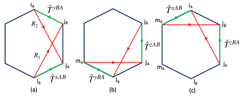
Figure 1: The configurations that give CS terms. The green lines represent the $\hat{T}$ matrices and red lines are associated with Green function elements.

$$\Delta S_{CS}=\frac{i}{4\pi}\text{sign}(\xi)\,\text{sign}(W^{\prime})\sum_{\langle\langle ee^{\prime}\rangle\rangle}\int d\tau A^{x}_{e}\frac{\partial A^{y}_{e^{\prime}}}{\partial\tau}.$$ (15)

The link pairs $ee^{\prime}$ are as in Fig. 1a. It is easy to obtain similar CS contributions from the diagrams in Fig. 1b and 1c. Note that the two link fields in our CS action are separated by precisely one link and do not share a vertex. The latter is a crucial difference from the phenomenological lattice CS action introduced in Ref. [43] for the special case of lattices with one-to-one face-vertex correspondence. The fact that we have explicitly constructed a lattice CS gauge theory for a chiral phase on the honeycomb lattice contradicts the claim in Ref. [43] that this is possible only for lattices with one-to-one face vertex correspondence. However this is in line with the understanding that lattice gauge theories for chiral fermions can be constructed by relaxing ultralocality [45, 46]. We have checked that Chern-Simons level matrix $K_{ee^{\prime}}$ is not singular. In the model, the sign of effective gap $W^{\prime}$ does not change unless $\kappa$ changes sign. However, $\text{sign}(\xi)$ is controlled by the strength of the Zeeman field. In the FM case, $\xi$ does not change sign with increasing Zeeman field, but in the AFM case it does. The sign change of the CS level between the low and intermediate field regime originates from a corresponding change in the chirality of the free Majorana band in the AFM case [17]. In our formalism, the $z$-links are associated with the gauge fields $A_{e}+B_{e}.$ Consequently, diagrams containing one $z$-link (e.g. Fig. 1b, 1c) also generate a correction to the mutual CS interaction:

$$\Delta S_{MCS}=\frac{i}{4\pi}\text{sign}(\xi)\,\text{sign}(W^{\prime})\sum_{\langle\langle ee^{\prime}\rangle\rangle}\int d\tau A^{y}_{e}\frac{\partial B^{z}_{e^{\prime}}}{\partial\tau}.$$ (16)

In the remaining part of the paper, we study the nature of the topological phases in different field regimes. For this purpose we go over to the continuum limit by taking the lattice constant $a\to 0$. The lattice gauge field $A_{e}$ is a line integral of the vector potential $\int_{e}\vec{A}.d\vec{l}.$ The lattice sum passes over to the continuum limit as $\sum_{\text{links}}=\frac{1}{V}\int d^{2}x,$ where $V=3\sqrt{3}a^{2}/2$ is the unit cell volume. The links are not orthogonal to each other; however in going to the continuum limit, the only nonvanishing CS interaction appears between orthogonal components of the vector potentials. We finally arrive at a continuum CS theory with two abelian gauge fields and a level matrix given by

$$K =\begin{bmatrix}\text{sign}(\xi)\,\text{sign}(W^{\prime})&1+\text{sign}(\xi)\,\text{sign}(W^{\prime})\\ 1+\text{sign}(\xi)\,\text{sign}(W^{\prime})&0\\ \end{bmatrix}.$$ (17)

At low fields ($0\leq h<h_{c1}$), $\text{sign}(\xi)\,\text{sign}(W^{\prime})=1,$ so $K_{\text{low}}=\begin{bmatrix}1&2\\ 2&0\\ \end{bmatrix}$. It is important to note here that $K_{\text{low}}$ differs from that of a $Z_{2}$ spin liquid for which $K_{Z_{2}}=\begin{bmatrix}0&2\\ 2&0\\ \end{bmatrix}.$ In the AFM case for $h_{c1}\leq h<h_{c2},$ we get $\text{sign}(\xi)\,\text{sign}(W^{\prime})=-1$ and $K_{\text{inter}}=\begin{bmatrix}-1&0\\ 0&0\\ \end{bmatrix}$. At even higher fields $h>h_{c2}$ corresponding to the partially polarized phase, $\text{sign}(\xi)\,\text{sign}(W^{\prime})=0$ and we revert to the bare trivial $K$-matrix. For the FM phase, there is only a single phase transition at some $h_{c},$ from $K_{\text{low}}$ to the trivial one. Having obtained the level matrices in the different field regimes, we now describe the nature of these phases.

Consider first an abelian $Z_{2}$ topological order which corresponds to the matrix $K_{Z_{2}}.$ The abelian quasiparticles have the general form $X=e^{i\int_{C}l_{X}^{\alpha}A_{\alpha\mu}dx^{\mu}}$ where $l^{\alpha}_{X}\in{Z}$. Here $A_{1\mu}=A_{\mu}$ and $A_{2\mu}=a^{*}_{\mu}.$ Two different strings anticommute when they cross odd number times as a result of the commutation relations $[A_{\mu}(x),a^{*}_{\nu}(x^{\prime})]=2\pi i\epsilon_{\mu\nu}K^{-1}_{Z_{2}}\delta^{2}(x-x^{\prime})=\pi i\epsilon_{\mu\nu}\delta^{2}(x-x^{\prime}).$ The quasiparticle charges are

$$l_{e}=\begin{bmatrix}1\\ 0\\ \end{bmatrix},l_{m}=\begin{bmatrix}0\\ 1\\ \end{bmatrix},l_{\epsilon}=\begin{bmatrix}1\\ 1\\ \end{bmatrix},$$

and using these definitions together with the canonical commutation relations, one easily recovers the abelian fusion rules and braiding statistics. Quasiparticles are detected from the eigenvalues of the Wilson loops. The Wilson loop $e^{i\oint_{\mathcal{C}}\vec{A}\cdot d\vec{l}}$ gives $+1$ when it encloses the trivial quasiparticle $\mathbf{1}$ or the $e$ quasiparticle, and $-1$ otherwise. Similarly the Wilson loop $e^{i\oint_{\mathcal{C}}\vec{a^{*}}\cdot d\vec{l}}$ is $+1$ when it encloses $\mathbf{1}$ or the $m$ quasiparticle, and $-1$ otherwise. The $\epsilon$ particle corresponds to both the eigenvalues being $-1.$ For any kind of abelian phase the nature of the phase and all topological properties can be completely described by the abelian $K$ matrix. But that is not true in general for any non-abelian phase like Ising topological order (ITO) which we will describe now. In the region $0<h<h_{c1},$ where $K=K_{\text{low}},$ and $Z_{2}$ is clearly lost since the above fusion rules are no longer satisfied.

For an anyon model which is symmetric under some permutations of their topological charges (e.g. $e\leftrightarrow m$ for $Z_{2}$), one can describe a non-abelian phase by introducing twist defects [47, 48, 49, 50] such as dislocations. This is related to a local symmetry operation $G=\begin{bmatrix}0&1\\ 1&0\\ \end{bmatrix}$ on $K_{Z_{2}}$ that amounts to interchanging the two species of gauge fields locally. For $Z_{2}$ topological order, it is known that such twist defects ($\sigma$) are nonabelian ITO anyons [47, 51].

In his original work, Kitaev made an analogy of his low-field Majorana mean field model with a chiral $p$-wave superconductor (a topologically trivial phase) where half-vortices are known to harbor Majorana zero modes that obey ITO braiding rules. However these nonabelian excitations are not intrinsic excitations of the mean field theory. The missing ingredient needed to detect intrinsic Majorana excitations is the dual gauge field.

Now we show that our $K_{\text{low}}$ provides a natural way to realize a twist defect that satisfies the ITO fusion rules. The diagonal entry in $K_{\text{low}}$ introduces a single twist that breaks $e$ and $m$ exchange symmetry. We show that the string $\Gamma=e^{i\oint_{c_{2}}\vec{a^{*}}\cdot d\vec{l}},$ where the closed loop $c_{2}$ winds twice (say anticlockwise) with only one crossing plays the role of detector of a twist defect $\sigma.$ This is analogous to the double winding string detectors of twist defects $\sigma_{\pm}$ in $Z_{2}$ spin liquids [47] - the main difference in the $Z_{2}$ case is the time reversal symmetry allows two distinct twist defects of opposite chirality, and respective eigenvalues $+i$ or $-i$ for the corresponding double winding detector. In our case, only one of these eigenvalues is realized because all defects have the same chirality. Mathematically, the imaginary eigenvalue for the double winding loop comes from the non-trivial commutation relation $[a^{*}_{\mu}(x),a^{*}_{\nu}(x^{\prime})]=2\pi i\epsilon_{\mu\nu}K^{-1}_{\text{low}}\delta^{2}(x-x^{\prime})=-\frac{\pi}{2}i\epsilon_{\mu\nu}\delta^{2}(x-x^{\prime})$ in our model. On the other hand, because of the presence of the diagonal term, $e$ and $m$ charges cannot be defined consistently. We now obtain the fusion rules of these twist defects. In the absence of other excitations, for two closed strings that wind twice, say $\Gamma_{1}$ and $\Gamma_{2},$ we have $\Gamma_{1}\Gamma_{2}=-1$ in Fig. 2 (a), where the minus sign comes from the presence of two nontrivial crossings, and the remaining dotted curve counts the fermion number parity within. The $\psi$ fermionic quasiparticle can be realised with the string, $e^{i2\int\vec{a^{*}}\cdot d\vec{l}},$ and introducing an $\psi$ into any double winding loop of the type $\Gamma$ simply changes the fermion number parity. The fermion number parity can be $\pm 1$ i.e., modulo $2,$ the charge within is $1$ or $\psi.$ In Fig. 2 (b), introduction of a $\psi$ (yellow line) into $\Gamma$ clearly does not change the sign, consistent with the fusion rule $\sigma\times\psi=\sigma.$

Now we define the Majorana fermion by an open string $C_{j}=e^{i\int\vec{a^{*}}\cdot d\vec{l}}$ that loops around a twist defect at $j$ and all Majorana strings thus defined are to have the same end points. Two such strings (say, $C_{j}$ and $C_{j+1}$) with same end points, when braided, results in the change in the orientation of their intersection, yielding the braiding relations $C_{j}\rightarrow C_{j+1},\,C_{j+1}\rightarrow-C_{j},$ consistent with Refs. [52, 47]. The total charge upon fusion is $-iC_{j}C_{j+1}$, taking values either $+1$ for 1 or $-1$ for $\psi$ respectively.

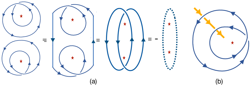
Figure 2: The blue and yellow line represent the string $e^{i\int\vec{a^{*}}.d\vec{l}}$ and $e^{i2\int\vec{a^{*}}.d\vec{l}}$ respectively. In (a) fusion of two closed strings that wind twice are shown. The dotted line measures the fermion number parity within. The fusion between the quasiparticles $\psi$ and $\sigma$ is shown in (b).

The anyon sector $\{\textbf{1},\psi,\sigma\}$ gives Ising topological order.

In anyon-CFT correspondence [53, 54, 55, 56], it is well known that these twist fields in $1+1$ dimensions are either holomorphic or antiholomorphic, which is the case for our model. From the edge theory one can also calculate the conformal weight of these fields and the braiding statistics of ITO. The GSD on the torus for this ITO phase is three due to three superselection sectors discussed above. The topological entanglement entropy ($\gamma$) can be expressed as $\gamma=\ln D$ where $D$ is the total quantum dimension. In case of the ITO, $D^{2}=\sum_{\alpha}d^{2}_{\alpha}$ with $d=1$ for vacuum and $\psi$ and $d=\sqrt{2}$ for quasi-particle $\sigma,$ hence $\gamma=\ln 2$ in ITO as expected. On the other hand, the field regime $h_{c1}\leq h<h_{c2}$ corresponds to a topologically trivial chiral abelian phase with fermionic bulk excitations, so $D=1,\,\gamma=0.$ Note that in the ITO phase, strings composed of the gauge field $A_{\mu}$ do not have any nontrivial commutation relation with the $\sigma$ or $\psi$ quasiparticles of ITO. On the other hand, in the intermediate phase of AFM Kitaev model, they are the sole gauge fields, and give the parity and time reversal symmetry breaking CS term in the theory. The gauge sector gives nontrivial contribution to the central charge in this regime, and is associated with the nonzero vison Chern number.

We finally discuss the chiral central charge $(c)$ of the edge theory in the different field regimes. From the bulk-edge correspondence [57, 58, 59], the effective edge theories of $K_{\text{low}}$ imply the following Kac-Moody algebra of chiral bosons ($\phi$),

$$[\phi_{I}(x),\partial_{y}\phi_{J}(y)]=\pm 2\pi i{K^{-1}_{\text{low}}}_{I,J}\delta(x-y).$$ (18)

The fact that number of positive and negative eigenvalues are equal, results in same number of left-movers and right-movers on the edge, corresponds to zero net chirality ($c=0$). Thus the central charge in the ITO phase, coming solely from bare chiral Majoranas is $\frac{1}{2}$ [59]. On the other hand, the intermediate phase of AFM Kitaev model, has an effective abelian CS theory of level $k=-1$ and leads to $c=-1$ from the edge theory [59], while for the bare chiral majoranas, the Chern number (-1) is flipped w.r.t. the low field phase [17]. The resultant chiral central charge in this phase taking into account both the Majorana and gauge sectors is $c=c_{\text{Majorana}}-c_{\text{gauge}}=\frac{1}{2}.$ Remarkably, this topologically trivial phase has the same $c=\frac{1}{2}$ as the ITO phase at lower fields, implying that the half-quantized thermal Hall effect persists with no change in sign, which contradicts the expectation of a change of sign of the thermal Hall effect [17] purely from the parton sector.

Discussion: In summary, we presented a microscopic derivation of abelian lattice Chern-Simons gauge theories for the FM and AFM Kitaev models subjected to time reversal symmetry breaking Zeeman (001) and scalar spin chirality perturbations. We obtained a comprehensive understanding of the topological phases and emergent excitations in different field regimes. In the low field phase, which is long known to have ITO, we constructed the nonabelian $\sigma$ anyons as twist defects of a specific chirality. These anyons arise naturally in our gauge theory as intrinsic bulk excitations unlike previous work that was based on manually creating half-vortex excitations in analogy with the chiral $p$-wave superconductors that do not have ITO. In the AFM case, the intermediate field phase was found to be chiral and with trivial topological order. The chiral central charge was found to be $\frac{1}{2}$ (same as the ITO phase, with no sign change). Remarkably, this trivial phase is predicted to give the same half-quantized thermal Hall response as the nonabelian ITO phase that exists at lower fields. The gauge fluctuations were found to strongly affect all the topological properties of the intermediate field regime when compared to earlier parton mean field treatments. Our technique provides a way for understanding other open questions, e.g. the possibility of field-revived ITO in the simultaneous presence of competing ITO degrading perturbations such as Zeeman and exchange interactions.

Our CS fermionization approach is generally applicable to 2D spin-$1/2$ systems with fermion number parity symmetry, and could be useful in understanding the effects of perturbations on the stability and phase transitions in different spin liquid systems.

The authors acknowledge support of the Department of Atomic Energy, Government of India, under Project Identification No. RTI 4002, and Department of Theoretical Physics, TIFR, for computational resources. JD and VT thank specially Subir Sachdev for useful comments on an earlier version of this work, and Shiraz Minwalla, Ashvin Vishwanath, Yuan-Ming Lu, and Nandini Trivedi for fruitful discussions. JD also thanks Aman Kumar for numerical clarifications.

Appendix

Chern-Simons fermionization of spins using two abelian gauge fields and Majorana Mean-field theory

In the case of honeycomb Kitaev model, the Chern-Simons flux attachment is readily implemented for spins expressed in $SO(3)$ representation. Following Ref. [32], we use the following $SO(3)$ representation of spins,

$$\sigma^{x}_{i}=\gamma_{i}\eta^{x}_{i},\hskip 36.135pt\sigma^{y}_{i}=\gamma_{i}\eta^{y}_{i}\,\hskip 36.135pt\sigma^{z}_{i}=\gamma_{i}\eta^{z}_{i};$$ (19)

where $SO(3)$ singlet operator $\gamma_{i}=-i\eta^{x}_{i}\eta^{y}_{i}\eta^{z}_{i}$. This singlet operator commutes with the Majorana fermions at same site and anticommutes with other majoranas. This property leads to the following commutation relation for any $i$ and $j$ ,

$$[\gamma_{i},\sigma^{\alpha}_{j}]=0,$$ (20)

with $\alpha=x,y,z.$ Thus $\gamma_{i}$ are constants of motion that commute with any spin Hamiltonian. Upon bosonization, the corresponding constraint $\gamma_{i}\gamma_{j}=-i$ is enforced by the gauge theory.

Note that the number of gauge fields is doubled since dual lattice is also taken into account in Eq. 2. This is necessary for consistent formulation of CS theory on the honeycomb lattice. The level $k=1$ for the topologically trivial phase. Commutation relations of chains follow from the canonical commutation relations in Eq. (3) and the Baker-Hausdorff-Campbell formula:

$$\left[\int_{\mathcal{C}}A_{e},\int_{\mathcal{C}^{*}}a^{*}_{e^{*}}\right] =i\frac{2\pi}{k}\nu[\mathcal{C},\mathcal{C}^{*}],$$ (21)

where $\nu[\mathcal{C},\mathcal{C}^{*}]$ is the difference of right handed and left handed intersections of chains $\mathcal{C}$ and $\mathcal{C}^{*}.$ Correspondingly, the commutation of the respective Wilson lines will give

$$W_{\mathcal{C}}W_{\mathcal{C}^{*}} =e^{-i\frac{2\pi}{k}\nu[\mathcal{C},\mathcal{C}^{*}]}W_{\mathcal{C}^{*}}W_{\mathcal{C}}.$$ (22)

We now require to fermionize the spin degrees of freedom by attaching Wilson lines to the fermions so that spin commutation algebra is obeyed. This cannot be done using only one of the two gauge fields since the only nontrivial canonical commutation relation of the gauge fields is between $A_{e}$ and the corresponding dual $a_{e*}^{*}.$ From the CS fermionisation, the singlet operator in Eq. 19, is expressed as a Wilson line starting from any reference point $(c)$ to $i$ as $\gamma_{i}=e^{i\int^{i}_{c}(A_{e}+B_{e})}.$ The $B_{e}$ is a specific combination of dual lattice gauge fields shown in the Fig. 3.

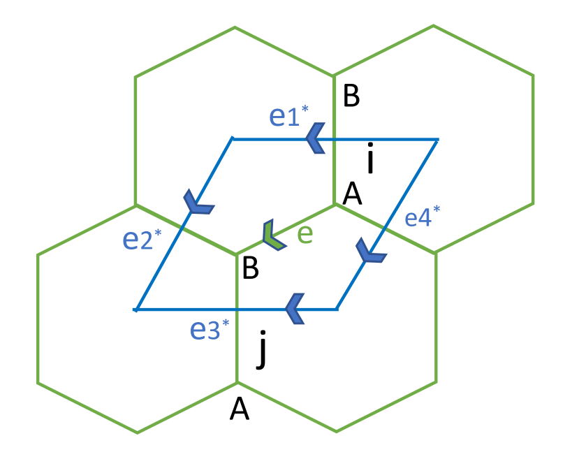
Figure 3: Anyonic (bosonic) exchange statistics of JW fermions on lattice sharing link $e=i_{A}\rightarrow j_{B}$ is implemented in the mutual CS formulation by attaching the fermionic bilinear to a holonomy $e^{iB_{e}},$ where $B_{e}$ is proportional to the sum of the four dual link potentials. Here $i,j$ are unit cells of the honeycomb lattice.

The spin commutation relations require the constraints in Eq. 5. Consider the string shown in Fig. (4) where the endpoint is at $i$. The $e^{i\int 2B}$ depends on the last two terms $e^{i2B_{e^{\prime}}}$ and $e^{i2B_{e}}$ associated with the links $e^{\prime}$ and $e$ respectively. The other terms are unity as all the dual fields correspond to these terms are counted twice. So $e^{i\int 2B}=1$ as $e^{i2B_{e^{\prime}}}=-1$ and $e^{i2B_{e}}=-1.$ The possible mean field configurations satisfying the condition $e^{i(2B_{e})}=-1$ are shown in the Fig. 5. The mean field for $A_{e}$ is zero. The gauge fluctuations are on top of the mean field choice.

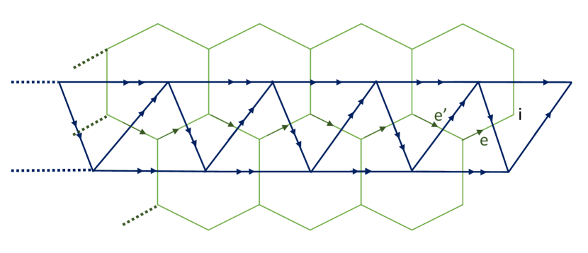
Figure 4: The string $e^{i\int_{e}2B_{e}}$ depends on the last two terms $e^{i2B_{e^{\prime}}}$ and $e^{i2B_{e}}$ live on the links $e^{\prime}$ and $e$ respectively. The other terms are unity as all the dual fields correspond to these terms are counted twice.

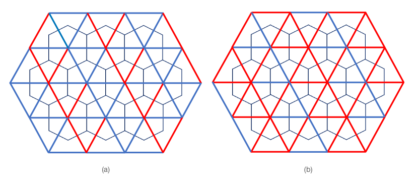
Figure 5: The configurations correspond to $e^{2iB_{e}}=-1$ where the $a^{*}_{e}$ on the red (blue) link is $\pi$ (zero) for the dual triangular lattice.

Effect of gauge fluctuations and level renormalization of Chern-Simons theory

We now beriefly describe the steps leading to the effective gauge theory. The bosonized action is

$$S_{\text{eff}}=-\frac{1}{2}\text{Tr}\ln\{G^{-1}_{0}+T\}+S_{CS}+NK_{z}\delta\Delta+NK_{z}m^{A}_{i}m^{B}_{i}.$$ (23)

Here $G^{-1}_{0}=(-i\omega_{n}+\mathcal{M}_{K})$ is the inverse Green function corresponding to the mean-field Hamiltonian (i.e. without the gauge fluctuations). The matrix $\hat{T}$ contains the gauge fluctuation parts of both Kitaev and the scalar spin chirality term and has the following form,

$$\hat{T}^{x}\! \!=\!\frac{1}{2}\begin{bmatrix}0&0&0&0\\ 0&0&0&0\\ 0&0&\kappa\delta{A^{x}_{e}}&KA^{x}_{e}\\ \!0&0&0&-\kappa\delta{A^{x}_{e}}\!\end{bmatrix},\hat{T}^{y}\!=\!\frac{1}{2}\begin{bmatrix}0&0&0&0\\ 0&0&0&0\\ 0&0&-\kappa\delta{A^{y}_{e}}&KA^{y}_{e}\\ \!0&0&0&\kappa\delta{A^{y}_{e}}\\ \!\end{bmatrix},$$

$$\hat{T}^{z} =\frac{1}{2}\begin{bmatrix}0&0&0&0\\ 0&0&0&0\\ 0&0&0&K\delta\varphi^{z}_{e}\\ \!0&0&0&0\\ \!\end{bmatrix},\hat{T}_{\langle\langle ij\rangle\rangle} \!\!\!=\frac{1}{2}\begin{bmatrix}0&0&0&0\\ 0&0&0&0\\ 0&0&\kappa\phi_{e}&0\\ \!0&0&0&-\kappa\phi_{e},\\ \!\end{bmatrix}.$$ (24)

Here $\hat{T}^{x},\hat{T}^{y},\hat{T}^{z}$ are the matrices with gauge fluctuations for $x$-link, $y$-link and $z$-link respectively and $\varphi^{z}_{e}=A^{z}_{e}+B^{z}_{e}.$ There is also another type of $\hat{T}_{\langle\langle ij\rangle\rangle}$ matrix associated with $i$ and $j,$ which are two next nearest neighbour unit cells and $\phi_{e}=A^{x}_{e}+A^{y}_{e}.$

Expanding the trace in Eq. (23) the first nontrivial contribution will come from $\text{tr}(G_{0}TG_{0}T)$ which is

$$\text{tr}\!=\!\!\int d{\tau}d{\tau^{\prime}}\!\!\sum_{i,j,k,l}\!\!G^{ij}_{0}(\tau-\tau^{\prime})T^{jk}(\tau^{\prime})G^{kl}_{0}(\tau^{\prime}-\tau)T^{li}(\tau).$$ (25)

All the matrices are of $4\times 4$ dimension. The Green function $G_{0}(ij)$ can be transformed to momentum space and frequency space via the following transformation:

$$G_{0}({\tau-\tau^{\prime}}) =\frac{1}{\beta}\sum_{m}G_{0}(i\omega_{m})e^{-i\omega_{m}(\tau-\tau^{\prime})}$$

$$\text{and}\hskip 3.61371ptG^{ij}_{0}=G_{0}(\vec{r}_{i}-\vec{r}_{j})=\frac{1}{V}\sum_{\vec{k}}G_{0}(k)e^{-i\vec{k}\cdot(\vec{r}_{i}-\vec{r}_{j})}.$$ (26)

Here

$$G_{0}=\begin{bmatrix}-i\omega_{n}&\frac{i{K}{\Delta}}{2}&-\frac{i({Km^{A}_{i}+h})}{2}&0\\ -\frac{i{K}{\Delta}}{2}&-i\omega_{n}&0&-\frac{i({Km^{B}_{i}+h})}{2}\\ \frac{i({Km^{A}_{i}+h})}{2}&0&-i\omega_{n}+\frac{W}{2}&\frac{-iKf}{2}\\ 0&\frac{i({Km^{B}_{i}+h})}{2}&\frac{iKf^{*}}{2}&-i\omega_{n}-\frac{W}{2}\\ \end{bmatrix}^{-1}.$$ (27)

Now let’s calculate $\text{tr}(G_{0}TG_{0}T)$ for an $x$-bond $i_{A}\rightarrow j_{B}$ ;

$$\text{tr}(G_{0}TG_{0}T) \!=\!\frac{1}{\beta^{2}V^{2}}\!\!\sum_{A,B}^{k_{1},k_{2},m,n}\!\!\int\!d\tau d\tau^{\prime}e^{-i\omega_{n}(\tau-\tau^{\prime})}e^{-i\omega_{m}(\tau^{\prime}-\tau)}$$

$$\times G^{AA}_{0}(k_{n}){T^{x}}^{AB}(\tau^{\prime})G^{BB}_{0}(k_{m}){T^{x}}^{BA}(\tau).$$ (28)

For simplicity we expand the dispersion around the Dirac points. Going over to the average and relative time coordinates, $\tau=\tau_{c}+\frac{\tau_{r}}{2}$ and $\tau^{\prime}=\tau_{c}-\frac{\tau_{r}}{2}$ we get the following link term in the effective action for $x$-bond at low temperature;

$$\mathcal{L}_{x}=\frac{1}{E_{c}}\left(\frac{\partial A^{x}_{e}}{\partial\tau_{c}}\right)^{2}\hskip 14.45377pt\text{with}\hskip 14.45377ptE_{c}\approx\frac{W}{2}\frac{\left[\Delta^{2}+(m+\frac{h}{K})^{2}\right]^{2}}{(m+\frac{h}{K})^{2}}.$$ (29)

The effective action coming from $y-$ bond has also a similar form. The corresponding contribution from the $z-$ bond is

$$\mathcal{L}_{z}=\frac{\delta^{2}}{E_{c}}\left(\frac{\partial(A^{z}_{e}+B^{z}_{e})}{\partial\tau_{c}}\right)^{2}.$$ (30)

These terms are essentially electric field like Maxwell terms of a lattice gauge theory. At high fields $h/K\gg 1,$ the electric coupling constants scale as $E_{c}\approx\frac{h^{3}}{K^{2}}$. We also find that the order parameter $\delta$ in Eq. 30 vanishes after the second phase transition (at $h_{c2}$) for AFM case and after $h_{c}$ for FM case. The vanishing of $\delta$ at high fields decouples the $xy$ link backbones making the system effectively one-dimensional. This dimensional reduction is also known from earlier mean field and spin wave studies. The leading contribution to the magnetic part of the Maxwell theory will come in the fourth order in $h/K,$ which we neglect since our interest is in the regime $h/K\lesssim 1.$

There is another second order contribution shown in Fig. 1 that results in a topological interaction of pairs of links. Let’s calculate $\text{tr}(G_{0}\hat{T}G_{0}\hat{T})$ for Fig. 1(a). The explicit expression for the configuration shown in 1(a) is

$$\frac{1}{\beta^{2}V^{2}}\sum_{\omega_{m},\omega_{n}}^{k_{m},k_{n}}\int d\tau d\tau^{\prime}e^{-i\omega_{n}(\tau-\tau^{\prime})}e^{-i\omega_{m}(\tau^{\prime}-\tau)}G^{AA}_{0}(k_{n})$$

$$\times\hskip 3.61371pt\hat{T}^{xAB}(\tau^{\prime})G^{BB}_{0}(k_{m})\hat{T}^{yBA}(\tau)e^{-i\vec{k_{n}}\cdot\vec{R_{2}}}e^{-i\vec{k_{m}}\cdot\vec{R_{1}}}.$$ (31)

The Green function elements are $G^{AA}_{0}(k_{n})=\frac{i\omega_{n}A+B}{(-i\omega_{n})^{2}-{E^{k_{n}}}^{2}}$ and $G^{BB}_{0}(k_{m})=\frac{i\omega_{m}A-B}{(-i\omega_{m})^{2}-{E^{k_{m}}}^{2}}$, where $A\approx\frac{\Delta^{2}+(m+\frac{h}{K})^{2}}{(\delta-\Delta-\xi)^{2}}$ , $B\approx\frac{W\Delta^{2}}{2(\delta-\Delta-\xi)^{2}}.$ We expand the dispersions around the Dirac points and perform the momentum integral resulting in

$$=-\frac{WAB}{4\beta V}\sum_{\omega,q\to 0}\frac{\omega}{2\pi}\frac{A^{x}_{e}(-i\omega)A^{y}_{e^{\prime}}(i\omega)}{\text{Vol of BZ}}$$

$$\times\hskip 1.8063pt\int^{\infty}_{-\infty}d\omega^{\prime}\int^{\pi}_{-\pi}dk_{x}\int^{\frac{2\pi}{\sqrt{3}}}_{-\frac{2\pi}{\sqrt{3}}}dk_{y}\frac{\sin k_{0}}{\left[{\omega^{\prime}}^{2}+v^{2}_{x}k^{2}_{x}+v^{2}_{y}k^{2}_{y}+W^{\prime 2}\right]^{2}},$$ (32)

where $\omega_{n}=\omega^{\prime},$ $\omega_{n}-\omega_{m}=\omega,$ and $k_{n}=k,$ $k_{n}-k_{m}=q.$ We have taken $\frac{1}{\beta}\sum_{\omega}=\frac{1}{2\pi}\int^{\infty}_{-\infty}d\omega$ and $\frac{1}{V}\sum_{k}=\frac{1}{\text{vol of BZ}}\int^{\pi}_{-\pi}dk_{x}\int^{\frac{2\pi}{\sqrt{3}}}_{-\frac{2\pi}{\sqrt{3}}}dk_{y}$ and $W^{\prime}=\frac{W\Delta}{2|(\delta-\Delta-\xi)|}$ is the effective gap. Let’s rescale the momenta by $k_{x}\rightarrow v_{x}k_{x}$ and $k_{y}\rightarrow v_{y}k_{y}$ and perform the integrations. The result is

$$\text{tr}(G_{0}TG_{0}T)\!=\!\frac{1}{\beta V}\frac{1}{4\pi}\text{sign}(\xi)\,\text{sign}(W^{\prime})\!\!\!\!\sum_{\omega,\langle\langle ee^{\prime}\rangle\rangle}\!\!\!\!\omega{A^{x}_{e}(-i\omega)A^{y}_{e^{\prime}}(i\omega)},$$ (33)

in frequency space and, re-expressing in Euclidean time, we find that the bare CS interaction of Eq. 2 now acquires the corrections

$$\Delta S_{CS} =\frac{i}{4\pi}\text{sign}(\xi)\,\text{sign}(W^{\prime})\sum_{\langle\langle ee^{\prime}\rangle\rangle}\int d\tau A^{x}_{e}\frac{\partial A^{y}_{e^{\prime}}}{\partial\tau}$$

$$\Delta S_{MCS} =\frac{i}{4\pi}\text{sign}(\xi)\,\text{sign}(W^{\prime})\sum_{\langle\langle ee^{\prime}\rangle\rangle}\int d\tau A^{y}_{e}\frac{\partial B^{z}_{e^{\prime}}}{\partial\tau}$$ (34)

to the diagonal and mutual interactions.