Approximation of sea surface velocity field by fitting surrogate two-dimensional flow to scattered measurements

Abstract

In this paper, a rapid approximation method is introduced to estimate the sea surface velocity field based on scattered measurements. The method uses a simplified two-dimensional flow model as a surrogate model, which mimics the real submesoscale flow. The proposed approach treats the interpolation of the flow velocities as an optimization problem, aiming to fit the flow model to the scattered measurements. To ensure consistency between the simulated velocity field and the measured values, the boundary conditions in the numerical simulations are adjusted during the optimization process. Additionally, the relevance of quantity and quality of the scattered measurements is assessed, emphasizing the importance of the measurement locations within the domain as well as explaining how these measurements contribute to the accuracy and reliability of the sea surface velocity field approximation. The proposed methodology has been successfully tested in both synthetic and real-world scenarios, leveraging measurements obtained from GPS drifters and HF-radar systems. The adaptability of this approach for different domains, measurement types and conditions implies that it is suitable for real-world submesoscale scenarios where only an approximation of the sea surface velocity field is sufficient.

[riteh]organization=Faculty of Engineering, University of Rijeka,addressline=Vukovarska 58, city=Rijeka, postcode=51000, country=Croatia

[cnrm]organization=Center for Advanced Computing and Modelling, University of Rijeka,addressline=Radmile Matejčić 2, city=Rijeka, postcode=51000, country=Croatia

1 Introduction

The significance of oceanic data became more evident as scientists established a connection between changes in oceanic circulation patterns and shifts in the global climate. To gather such data, satellite tracking of deployed drifters has emerged as a preferred method due to its cost-effectiveness in providing velocity data, compared to the amount of data collected from ships and ports. Consequently, over the past two decades, the deployment of drifters at various oceanic locations has increased substantially [1]. Between 1994 and 1995, the Gulf of Mexico witnessed the deployment of 300 satellite-tracked drifters. The data collected from this deployment has been thoroughly analyzed and documented in numerous publications [2, 3].

Similarly, satellite-tracked drifters were deployed in the semi-enclosed Adriatic Sea to determine the circulation properties [4, 5]. Over 200 drifters were deployed in the Adriatic Sea between 1990 and 1999, serving both academic and military purposes. The collected data was utilized to reconstruct an Eulerian velocity field of the Adriatic Sea. This involved interpolating velocities at the drifter locations through the use of cubic splines [6]. Due to the scope and measurement time-frame, this type of data can be used to reconstruct surface circulation in relation to wind forcing, river runoff, and bottom topography [7].

Typically, drifters can be advected across expansive areas exceeding 2000 square kilometers while the precision of the reconstructed velocity field is heavily reliant on the spatial coverage of the drifter paths [8]. Reconstruction of surface velocity fields in submesoscale processes, which occur at domain scales ranging from 0.1 to 10 kilometers and time scales ranging from 1 to 100 hours, cannot be resolved with satellite altimeters and observations by ships. A novelty in this area was The Lagrangian Submesoscale Experiment (LASER) which provided measurements of the surface velocity field in the northern Gulf of Mexico with high resolution in space and time [9]. A central aspect of this experiment involved releasing over 1000 surface drifters in submesoscale domains. Released drifters were predominantly biodegradable and were outfitted with drogues to negate the impact of wind and waves. The deployment density of these drifters facilitates the capture of scales ranging from tens of kilometers down to tens of meters.

In the last decade, interest in Lagrangian data for operational modeling such as search and rescue, the spread of pollutants and forecasting has increased significantly. This type of data makes it possible to define models that can predict the future behavior of surface currents, which in some cases can save lives. Two relevant approaches have been considered for the reconstruction and assimilation of Lagrangian data. The first approach is based on the estimation of velocities along trajectories as a ratio between observed position differences and time increments [10] and the direct use of these velocities to correct the model results. The second approach introduces an observational operator based on the particle advection equation and corrects the Eulerian velocity field by minimizing of the difference between observed and modeled trajectories [11].

The primary issue with Lagrangian drifter data stems from the fact that the drifters move with the oceanic flow, hence they are not evenly spread out and have a tendency to either cluster or move out of areas of interest. Furthermore, Lagrangian data describes trajectories that vary in space and time, while commonly specific fields, e.g. temperature and velocity, are of interest. Transitioning from trajectory analysis, the focus in this domain often shifts towards the detailed reconstruction of Eulerian velocity fields, where research papers emphasize the use of drifter data for velocity field reconstruction [12, 13, 14].

A study by [15] estimated the velocity field based on drifter data using a procedure that statistically interpolates the collected data both spatially and temporally. The authors concluded that as the distance between the drifters changes with the flow, the resolution they provide can vary in space and time, leading to interpolation errors. Velocity field estimations at similar submesoscales with high resolution are presented in [16, 9, 17]. Common methods for flow reconstruction often use least squares regression to reconstruct the flow field, or basic interpolation to find the minimum-energy solution that is consistent with the measured data. However, this approach is susceptible to over-fitting and is sensitive to noise due to the presence of restricted and potentially corrupted measurements. A study by [18] presented a method for flow field reconstruction based on sparse representation in a library of examples which is well-suited to structured data with limited, corrupt measurements. This method can be extended to complex flow fields by decomposing the spatial domain and seeking localized sparse representations.

Lagrangian satellite-tracked are driven by ocean currents, which means there is minimal control over the location of the measurements. Furthermore, they provide limited coverage for a desired region. In contrast, Eulerian velocity data with global coverage can be obtained, but is limited by the spatial and temporal resolution of the satellite altimetry. In addition, altimetry measurements rely on smoothing and interpolation from base satellite measurements. The challenge associated with satellite measurements lies in their limited accessibility and occasional atmospheric interference. This has led to the widespread adoption of an alternative method for acquiring surface velocity employing high-frequency (HF) radar. This method utilizes electromagnetic waves to measure surface currents in near-real-time. [19] used HF-radar data to assimilate into a numerical model of the northwestern Mediterranean Sea. The assimilation process involved adjusting the model’s initial conditions and boundary conditions to match the observed surface currents. The study found that assimilating HF-radar data into the model improved the accuracy, particularly in areas where surface currents were difficult to measure.

While HF-radar technology provides notable advantages, it comes with certain limitations, such as restricted depth penetration, susceptibility to interference, and difficulties in achieving fine spatial resolution. To address these challenges, [20] used a genetic algorithm to optimize the boundary conditions and physical parameters of the model. The performance of the model, i.e. the optimized depth boundary condition, was compared to Multibeam Bathymetric data. In addition, the sensitivity of the model to various parameters such as bottom friction, eddy viscosity and the shape of the coastline was discussed. It was determined that bottom friction is the most influential parameter and was hence suggested that it should be carefully calibrated to improve the accuracy of the model.

Artificial Intelligence (AI) and machine-learning techniques have recently emerged as alternatives to traditional interpolation and optimization methods for flow field predictions, as discussed in [21]. Several studies, such as those by [22, 23], have explored the application of recurrent neural networks to analyze temporal patterns in drifter motion, providing reduced errors in drifter models. Additionally, a Transformer-based decoding architecture is utilized in [24] for flow field prediction, offering a fast and straightforward estimation without relying on extensive CFD simulations. Research presented by [25] introduced a Physics-Informed Neural Network (PINN) method in conjunction with the characteristic-based split (CBS) method, effectively solving shallow-water equations and making it applicable for ocean flow field estimation. Furthermore, an adaptive neuro-fuzzy inference system-based model is used in [26] to predict missing velocity vectors in fluid flow, a common occurrence during flow measurements. These AI and machine learning approaches have garnered significant attention in CFD, demonstrating notable success in turbulence modeling, shape optimization and flow field prediction.

In this study, a novel simulation-based optimization approach is introduced. By combining a simplified two-dimensional surrogate flow model and an optimization algorithm, the boundary conditions of a flow simulation can be adjusted, i.e. the velocity field can be aligned with the velocity values derived from the scattered drifters. The proposed approach leverages processing power to offset the need for extensive measurement data, hence this innovative concept requires a smaller number of drifters. The importance of such an algorithmic approach is not limited to academic research, as it can be adapted for use in search and rescue scenarios. By accurately estimating the velocity field in a given area, it enables the prediction of the movement of individuals or objects lost at sea. This capability is crucial for planning and executing rescue operations with greater precision and efficiency. Beyond search and rescue operations, the proposed simulation-based fitting approach emerges as a promising alternative to traditional methods of velocity field reconstruction, potentially demonstrating its versatility in diverse applications within the fields of fluid mechanics and ocean engineering.

2 Surrogate two-dimensional flow model

Models involving unsteady flows require substantial computational resources, resulting in prolonged simulation times. As this data is rarely of interest in large scale models, a surrogate flow model based on stationary incompressible flow has been adopted. Our methodology intentionally excludes influential phenomena such as wind, waves, changing tides, and temperature variations present in the sea flow. This deliberate omission positions our model as a tool for rapid approximation of sea surface flow. Despite these simplifications, our simulation-based optimization approach offers several advantages over traditional methods. A smaller number of drifters is required, considerably reducing the cost and time needed for data collection. Additionally, the approach relies on CFD simulations, enabling the capture of fluid flow physics and providing more accurate velocity fields. The suggested method is particularly valuable for applications requiring a comprehensive understanding of flow characteristics.

2.1 Stationary 2D flow model

The proposed stationary flow model describes the motion of fluids at low and medium velocities in a connected computational domain $\Omega\subset\mathbb{R}^{2}$ based on the incompressible Navier–Stokes equations [27, 28, 29]:

$$\rho\left(\mathbf{u}\cdot\nabla\mathbf{u}\right)-\nabla\cdot\left(2\mu\cdot\epsilon(\mathbf{u})\right)+\nabla p=\rho\mathbf{f}$$ (1)

$$\nabla\cdot\mathbf{u}=0$$ (2)

The vector $\mathbf{u}$ represents the fluid velocity, and $p$ denotes the fluid’s dynamic pressure. The rank-2 tensor $\epsilon(\mathbf{u})=\frac{1}{2}\left(\nabla\mathbf{u}+(\nabla\mathbf{u})^{\top}\right)$ defines the viscous stress tensor for an incompressible Newtonian fluid. Here, $\rho$ denotes fluid density, and $\mu$ represents the fluid’s dynamic viscosity. Density remains constant due to the assumption of incompressibility. The term $\mathbf{f}$ specifies external forces acting on the fluid.

To account for the interactions between the observed section of the sea and the broader sea domain, a specific combination of boundary conditions is employed. This combination ensures an adequate representation of the dynamic interactions at the boundary and increases the reliability of our computational model. The proposed model aims to reconstruct the velocity field by generating tangential velocities and pressure values at the boundary. However, these boundary values should not be randomly generated i.e. their range should reflect realistic circumstances in order to recreate the physics of a realistic flow. Therefore, the lower and upper velocity limits are set according to [30, 31, 32] where the surface velocities were estimated using a combination of data from radar, numerical models, and infrared satellite images of the Adriatic Sea. The authors noted that the surface currents are highly variable, with speeds ranging from less than 0.1 m/s to more than 0.5 m/s. The average surface velocities were around 0.1-0.2 m/s in most areas. Consequently, a range of -0.2 m/s to 0.2 m/s is used in our proposed approach.

Once the tangential velocities and total pressure values are set, the next step is to define velocity and pressure profile functions. This involves interpolating the tangential velocity and pressure values along the boundary length while ensuring that the values at the edges of the coastline are set to 0. This is then repeated in the optimization procedure until the boundary condition produces a velocity field that matches the velocity values of the drifter.

The turbulence is modeled using the k-$\omega$ shear stress transport model [33], which combines the strengths of the k-omega and k-epsilon turbulence models in order to enhance the accuracy and reliability of capturing complex turbulent flows. This hybrid approach divides the flow domain into two distinct regions: the near-wall region and the outer region. In the near-wall region, the model employs a wall-function approach, accurately capturing the near-wall turbulence behavior. In the outer region, the model acts as a free-stream model, providing reliable predictions of the turbulence characteristics away from the wall [34]. The turbulence variables ($k$, $\omega$) were computed using:

$$k=\frac{3}{2}(\left|\mathbf{u}\right|I)^{2}$$ (3)

$$\omega=\frac{k^{0.5}}{C_{\mu}^{0.25}L}$$ (4)

where $k$ is turbulence kinetic energy, $I$ is turbulence intensity (5%), $\omega$ is the specific dissipation rate, $C_{\mu}$ is a turbulence model constant and equals 0.09 while $L$ is the turbulent length scale.

2.2 Numerical implementation

The computational domain in considered test cases is either synthetic in nature or represents a realistic geographical region. For specific regions, the relevant data is obtained using Google Earth polygon extraction (available on Google Earth) and noted accordingly. Upon extracting polygons, the generation of an STL model becomes essential for the subsequent creation of a numerical mesh. A corresponding two-dimensional numerical mesh is then created using cfMesh [35] and implemented in an open-source CFD package OpenFOAM [36]. Given that equations 1 and 2 are applied to steady-state incompressible flow, simulations utilize the simpleFoam solver implemented within OpenFOAM. This solver employs a semi-implicit method for pressure-linked equations (SIMPLE) [37]. In terms of boundary conditions, we treat the coastline as a solid wall by applying a no-slip (Dirichlet) boundary condition. When fluid flows out of the domain at a boundary face, the boundary condition for velocity is defined as the Neumann boundary condition, meaning that the velocity of the fluid at the boundary is extrapolated to the velocity inside the domain. When fluid flows into the domain, the open sea boundary switches to a Dirichlet boundary condition, where the velocity is calculated based on the flux in the patch-normal direction. Additionally, we defined tangential velocities because the flow entering a domain is not necessarily perfectly aligned with the inlet boundaries. Specifying a tangential velocity helps simulate more realistic inlet flow conditions, taking into account any swirl or tangential motion in the fluid.

The pressure at the open sea boundary is defined using the Dirichlet boundary condition with a set range of values while the coastline is defined using Neumann boundary condition. To ensure that the pressure value within the domain is well-defined, a reference cell is selected and assigned a pressure value of zero. This reference cell serves as a reference point for the pressure gradient calculations throughout the domain.

Incorporating the k-$\omega$ shear stress transport model into our modeling strategy, we defined turbulence values at the coastline using wall functions, while for the open sea, we specified the Neumann boundary conditions. Boundary conditions for all test cases are briefly summarized in Table 1.

Table 1: An overview of the boundary conditions employed

Field	Inlet/Outlet	Coastline
$u$	pressureInletOutletVelocity	noSlip
$p$	totalPressure	zeroGradient
$k$	fixedValue	kqRWallFunction
$\omega$	fixedValue	omegaWallFunction

Second-order accuracy was predominantly employed in OpenFOAM simulations, with second-order gradient and Laplacian schemes. Notably, first-order schemes (Gauss upwind) were selectively used for divergence terms related to convective transport to enhance stability in regions of steep gradients. Time derivatives and interpolations were treated with default second-order and linear schemes, respectively, while the meshWave method calculated distances to the nearest wall. The described boundary conditions and overall setup were kept the same for all test cases.

3 Model fitting and optimization problem formulation

The concept of model fitting implies an iterative procedure to determine velocity and pressure functions at the domain boundaries. These functions define the boundary values that induce various types of flows within the domain. The objective of the model fitting process is to minimize the disparity between the results obtained using CFD and sparse measurements. Therefore, in order to formulate the optimization problem, functions need to be parameterized i.e. the optimization vector needs to be defined.

3.1 Boundary condition parametrization

In the proposed approach, the optimization algorithm iteratively improves the values from the optimization vector to minimize the error value, i.e. to minimize the difference between the simulated flow field and the reference flow. As a result, the accuracy and reliability of the flow field reconstruction heavily rely on the optimization vector. This vector encompasses the values of tangential velocity and pressure at the boundary control points:

$$\mathbf{b}=\left(\mathbf{u}_{t,1},p_{1},\ldots,\mathbf{u}_{t,n_{CP}},p_{n_{CP}}\right)^{T}$$ (5)

where $n_{CP}$ is the number of boundary control points.

The locations of boundary control points where velocity and pressure values are specified can be uniformly or non-uniformly distributed, and their placement is determined based on the length of the boundary. A negative velocity value in the optimization vector signifies that the fluid is leaving the domain, whereas a positive value indicates that it is entering the domain. The velocity at the edges of the coastline is 0, as the wall has a no-slip condition. Further, the pressure values enable the computation of flux, a critical factor in determining velocity in the patch-normal direction. Consequently, the velocity at the boundary control point results from a combination of the tangential velocity set by the optimization algorithm and the velocity computed from the flux in the patch-normal direction.

In order to capture realistic flows, the bounds for optimization variables are set to -0.35 to 0.35 $m/s$ for tangential velocity and -0.05 to 0.05 $m^{2}/s^{2}$ for pressure at the boundary control points. Once the values are assigned to the boundary control points, cubic spline interpolation is used to obtain values (velocity and pressure) for each cell along the length of the boundary. Subsequently, during the optimization process, as the optimization vector changes, the velocity profile is iteratively updated until the output (error value) matches the target fitness. Visual representation of velocity profile with referent and optimized velocity vectors can be seen in Figure 1 where a synthetic scenario called Simple bay case is created to showcase a workflow procedure on a domain with features outlined in Table 2. The simulation shows that certain parts of the domain, specifically the ones very close to the coastline, remain intact throughout the entire simulation. This means that the vortexes do not reach or impact those areas.

Table 2: Characteristics of the Simple bay test case

Case characteristics	Simple bay
Test case type	Synthetic
Domain area [$km^{2}$]	24.6
Number of boundaries	1
Total boundary length [$km$]	9.4
Coastline length [$km$]	9.1
Number of boundary control points	5
Max velocity in the domain [$m/s$]	1.2
Presence of coastline/islands	Coastline
Number of cells	4625
Average cell size [$m$]	73.02

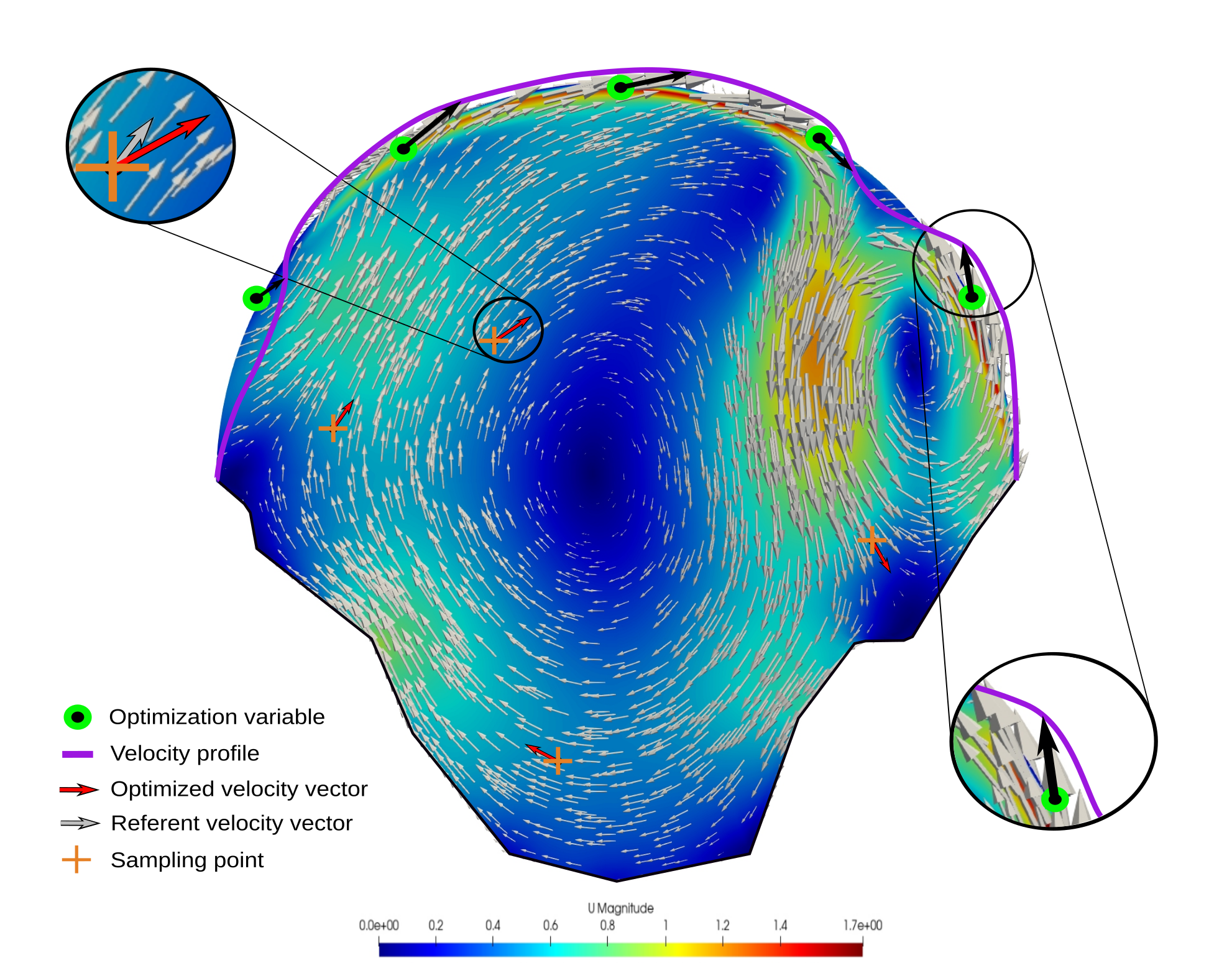
Figure 1: The figure illustrates the velocity profile generated using a specified optimization vector and how optimization variables (green dots) influence flow field reconstruction. The objective is to adjust the optimization variables until the red arrow (representing the current optimized velocity vector) aligns with the grey arrow (representing the reference velocity vector) for every sampling point (orange cross).

3.2 Objectives

A cost function is introduced to compute the difference between the reference values and calculated values. The reference values are discrete, point values, i.e. they are defined by their coordinates and corresponding velocity vector. During each evaluation, an OpenFOAM case is generated, where the entire velocity field is calculated. The velocity vectors at the coordinates of the sampling points representing the drifter locations are subsequently extracted.The cost function computes the drifter error $\epsilon_{d}$, using the equation:

$$\epsilon_{d}(\mathbf{b})=\dfrac{1}{n_{SP}}\sum_{i=1}^{n_{SP}}(\mathbf{u}_{r_{i}}-(\mathbf{u}_{s_{i}}(\mathbf{b})+\mathbf{u}_{w}^{*}))^{2}$$ (6)

where $n_{SP}$ is the number of sampling points, $\mathbf{u}_{r_{i}}$ is the reference velocity vector, $\mathbf{u}_{s_{i}}$ is the simulation velocity vector at sampling point location $\mathbf{s}_{i}$ and $\mathbf{u}_{w}^{*}$ is wind velocity vector.

Wind velocity vector is calculated through inner optimization for the entire field according to:

$$\mathbf{u}_{w}^{*}(\mathbf{b})= \underset{\mathbf{u}_{w}}{\text{argmin}}\left(\dfrac{1}{n_{SP}}\sum_{i=1}^{n_{SP}}(\mathbf{u}_{r_{i}}-(\mathbf{u}_{s_{i}}(\mathbf{b})+\mathbf{u}_{w}))^{2}\right)$$ (7)

where optimization tools from SciPy [38] were used to find minimum values of $\mathbf{u}_{w}^{*}$. The computational time for inner optimization is negligible and has no important impact on the overall optimization process duration since it relies on a single surrogate model simulation parameterized with $\mathbf{b}$.

To assess the effectiveness of flow reconstruction, we introduced a field error variable, denoted as $\epsilon_{f}$, similar to equation 6. The values of the velocity vectors at these field points are used to validate the field reconstruction and are not utilized in the optimization process:

$$\epsilon_{f}(\mathbf{b})=\dfrac{1}{n_{FP}}\sum_{j=1}^{n_{FP}}(\mathbf{u}_{r_{j}}-(\mathbf{u}_{s_{i}}(\mathbf{b})+\mathbf{u}_{w}^{*}))^{2}$$ (8)

where $n_{FP}$ is the number of field points, $\mathbf{u}_{r_{j}}$ is reference velocity vector and $\mathbf{u}_{s_{j}}$ is the simulation velocity vector at the field point location.

Given that $\epsilon_{f}$ is solely used as observation, the primary optimization objective is represented by $\epsilon_{d}$, and this approach is consistently employed across all test case scenarios. In synthetic scenarios where the complete velocity field values are accessible, the number of field points can go up to the number of cells of the numerical grid. However, in real-case scenarios with a limited number of deployed drifters, there are no corresponding field points available to validate flow reconstruction. In such cases, the success of flow reconstruction relies solely on the data obtained at sampling points. If there is a substantial deployment of drifters (50 or more), or when sampling points represent HF-radar measurements (which consistently provide more than 50 data points), users have the flexibility to allocate percentage for sampling and the rest for field points.

3.3 Constraints

In order to attain viable solutions in the context of this simulation-based optimization approach, it is necessary to set appropriate constraints. In this approach, constraints effectively correspond to residuals, serving as a guide in the optimization process to achieve both reliability and precision in the simulation results. The pressure residual constraints, defined as:

$$r_{p}(\mathbf{b})\leq 1e^{-3}$$ (9)

help maintain consistent pressure values throughout the optimization, preventing pressure imbalances that could lead to unrealistic behavior. Velocity residual constraints, set as:

$$r_{\mathbf{u}}(\mathbf{b})\leq 1e^{-4}$$ (10)

restrict the velocity magnitude within a specified range, enabling controlled and physically feasible fluid motion. k residual constraints, set as:

$$r_{k}(\mathbf{b})\leq 1e^{-4}$$ (11)

ensure that the turbulent kinetic energy remains within acceptable bounds. The $\omega$ residual constraint, set as:

$$r_{\omega}(\mathbf{b})\leq 1e^{-4}$$ (12)

restricts the specific dissipation rate of turbulence, ensuring its consistency with the underlying physics. The optimization process is collectively influenced by these constraints, ensuring the preservation of physical realism, stability, and accurate representation of fluid dynamics. These 5 constraints remain consistent across all test case scenarios.

3.4 Multimodality

Initially, testing was performed on the widely studied cavity lid case problem. This scenario represents a situation in which a rectangular cavity (area of $1m^{2}$) is filled with fluid and the flow is induced by the movement of the lid defined with 3 control points. This motion triggers the formation of vortexes and recirculation zones, which we aim to reconstruct. Velocities were assessed at 100 sampling points for 100 different sampling scenarios where tangential velocity at the inlet was set from -2$m/s$ to 2 $m/s$. Results indicated that a velocity vector at a chosen sampling point can be induced by different combinations of boundary values. Consequently, achieving the desired reference velocity through optimization does not guarantee the accuracy of the flow field in its entirety. This observation is briefly described in Figure 2. Based on this observation, local search methods are deemed unsuitable for incorporation into our simulation-based optimization approach.

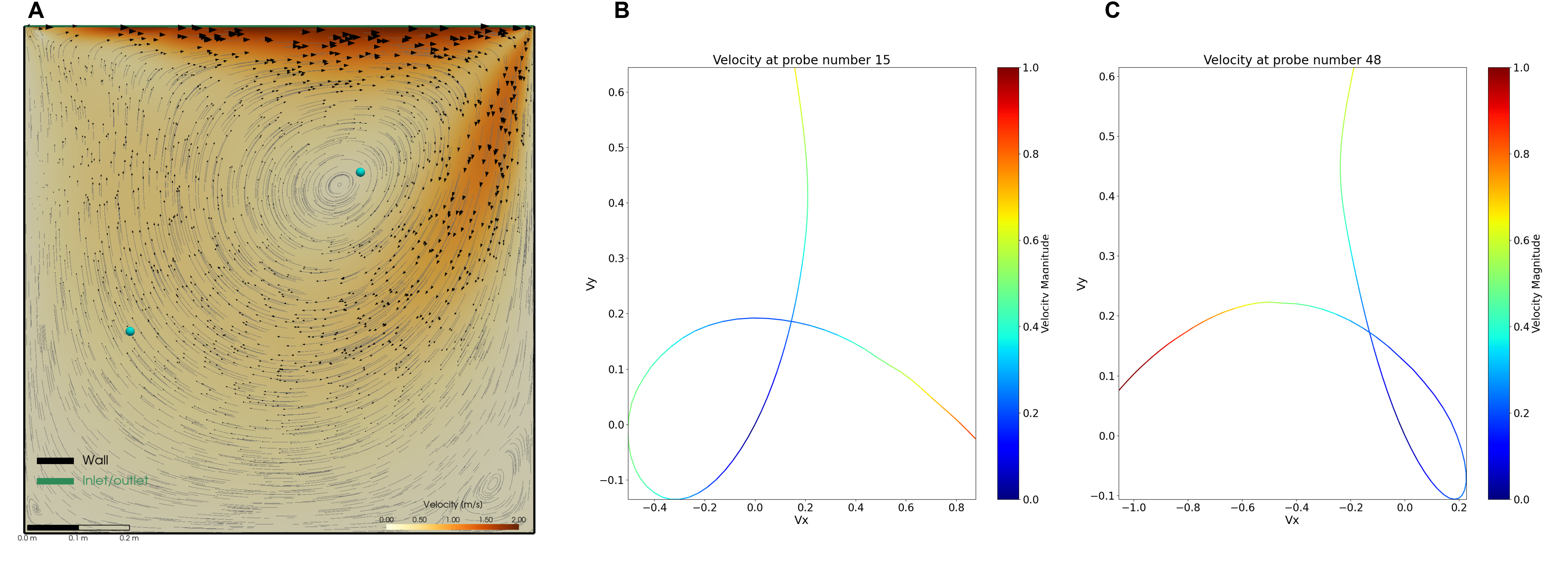
Figure 2: In total, 100 cavity lid cases are analyzed at 100 different sampling points within the domain to determine the multi-modality of the flow fitting problem. (A) Cavity lid case with a tangential velocity of 1.6 m/s, where the cyan-coloured dots represent two observation locations of 100 chosen for the multimodal investigation. (B) shows the velocity variation at sampling location 15 (the left point on (A)), with intersecting velocity curves showing that the same domain location can have the same velocity for different boundary conditions. (C) provides another example of intersecting velocity curves (the right point on (A)). When examining all sampling points over the entire range, it was concluded that certain locations within the domain had the same velocities for different optimization vectors. This finding suggests a multimodal nature of the problem indicating that different optimization vectors can lead to identical results.

4 Optimization methods and benchmark

After detailing the optimization process, the identification of the most suitable optimization algorithm for the proposed flow field reconstruction approach is performed. In order to evaluate the performance of various methods, a predefined threshold is established, enabling us to assess their efficiency, robustness, and scalability.

4.1 Analysis and Classification of Optimization Outcomes

The square difference of the velocities at sampling points, $\epsilon$_d, is used as a fitness function in all assessed optimization tests i.e. the optimization is defined as follows:

$$\underset{\mathbf{b}}{\text{minimize}} \epsilon_{d}(\mathbf{b})=\dfrac{1}{n_{SP}}\sum_{i=1}^{n_{SP}}(\mathbf{u}_{r_{i}}-(\mathbf{u}_{s_{i}}(\mathbf{b})+\mathbf{u}_{w}^{*}))^{2}$$ (13)

subject to $$\mathbf{b}_{l}\mathbf{\leq b}\leq\mathbf{b}_{u}$$

Convergence is considered achieved when the drifter error threshold $\epsilon$_d =0.0001 is reached. The flow field reconstruction error is additionally calculated for all optimization tests. The field error threshold is set to $\epsilon$_f =0.0003. $\epsilon$_f is only monitored and planned to be three times greater than the drifter error, maintaining a proportional difference for an accurate representation of the reconstructed flow. All results below these thresholds are deemed adequate.

Based on values computed for $\epsilon$_d and $\epsilon$_f , all optimization results can be classified into 4 distinct groups which are shown in Figure 3:

• $\epsilon_{d}$ > 0, $\epsilon_{f}$ > 0 (red area)

  A scenario where optimization failed to achieve the desired thresholds for both drifter and field error.

• $\epsilon_{d}$ > 0, $\epsilon_{f}$ $\approx$ 0 (gray area)

  An uncommon scenario where optimization successfully reaches the target threshold for field error but falls short in achieving the same for drifter error.

• $\epsilon_{d}$ $\approx$ 0, $\epsilon_{f}$ > 0 (orange area)

  A scenario where optimization effectively achieves the target threshold for drifter error, but the reconstructed field deviates from the reference field.

• $\epsilon_{d}$ $\approx$ 0, $\epsilon_{f}$ $\approx$ 0 (green area)

  The preferred scenario in which optimization successfully achieves target thresholds for both drifter and field error, signifying a successful reconstruction of the surface flow.

In order to determine the appropriate optimization algorithm for the proposed flow field reconstruction approach, an evaluation of the methods provided by the Python numerical optimization module Indago [39] was performed. Our aim was to determine the global search methods that best fit our modeling requirements, as we excluded local search methods due to the presence of multimodality explained in 3.4. Just to showcase the distinctions in optimization results between local and global search techniques, we used one gradient-free local search method Multi-Scale Grid Search (MSGS), an adaptation of Pattern Search within the Indago framework [39]. In contrast, for global search strategies, we used Particle Swarm Optimization (PSO) [40], Fireworks Algorithm (FWA) [41], and Artificial Bee Colony (ABC) [42] where the selection of these methods was guided by their specific strengths. PSO demonstrates proficiency in navigating expansive solution spaces, FWA excels in scenarios with multiple optima, and ABC proves effective in addressing constrained optimization problems, all well suited for our modeling approach [43].

For this investigation, five different Simple Bay test cases were created, each serving as a reference case. Each optimization algorithm was tested 10 times on each reference case, using 10 sampling points to reconstruct the flow field. This resulted in a total of 50 optimizations performed by each algorithm. Since this is synthetic scenario, wherein the case is predetermined and wind omitted, $\mathbf{u}_{w}^{*}$ is treated as 0. The results are shown in Figure 3.

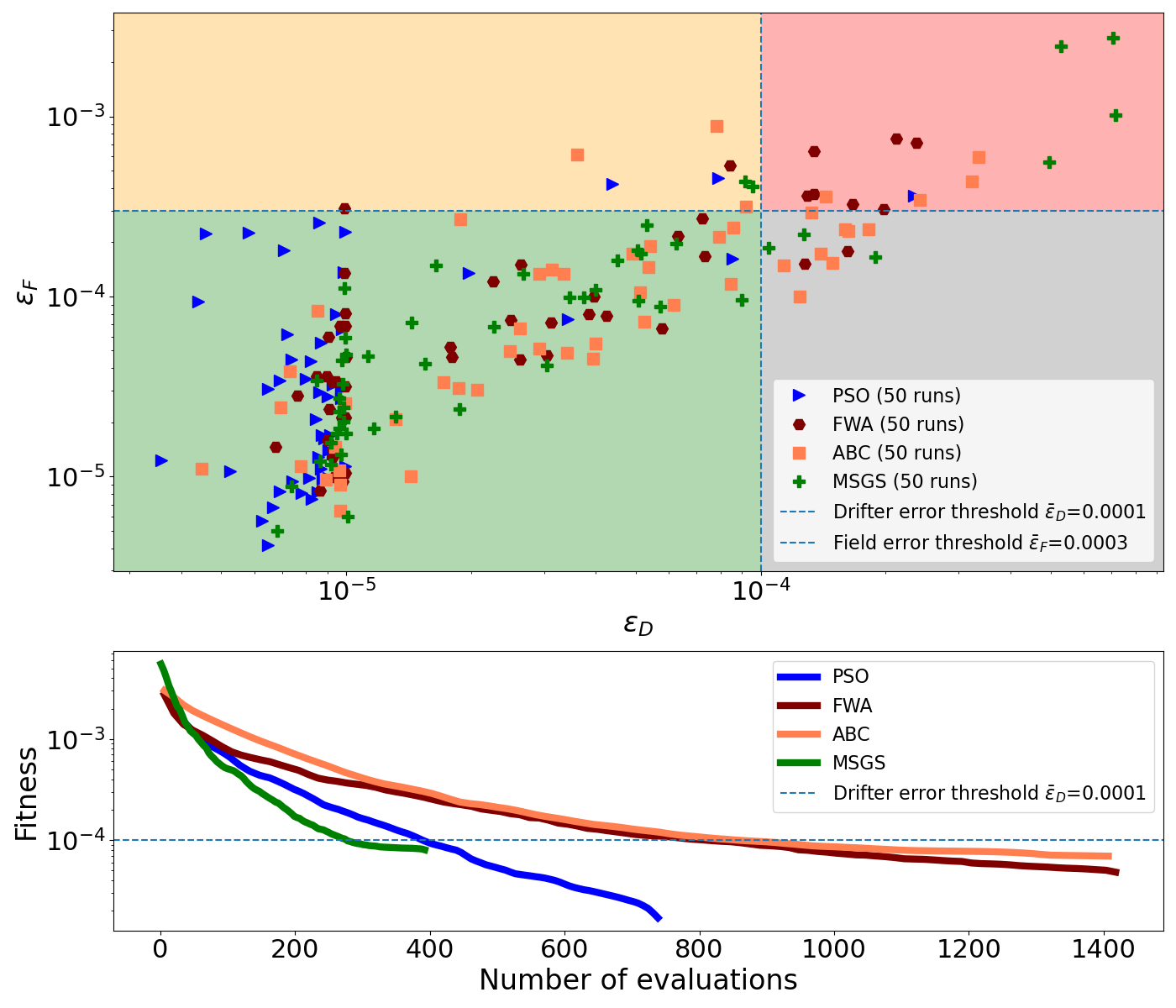
Figure 3: Algorithms used for numerical optimization and and their applicability for flow field reconstruction. The four colored squares represent four different result groups mentioned in the above text, with 6.8% of the results falling in the red area, 4% in the orange area, 5.2% in the grey area, and the majority, 84%, in the green area. The lower subplot shows the average convergence across all optimizations for each optimization algorithm. It is evident that MSGS, a local search algorithm, converges first. However, its overall fitness is on average worse than that of global search algorithms. Furthermore, compared to PSO, it often does not reach the specified threshold. PSO achieves an excellent balance between performance (second only to MSGS) and accuracy. This can be clearly seen from the narrow grouping (blue triangles) of results around $\epsilon_{d}$ = 1e-5. ABC and FWA demonstrate comparable fitness to MSGS, albeit with an extended optimization time.

It is evident that, on average, all methods successfully met the specified threshold, albeit at different speeds. The target objective threshold was intentionally reduced to 1e-5 in order to enhance the accuracy of the reconstructed field. Still, we retained a successful reconstruction threshold of 1e-4 for the optimization process, as indicated in the Figure 3. It is evident that, on average, all methods have successfully met the specified threshold, although at varying speeds. Notably, the local search technique MSGS demonstrated impressive speed, albeit with higher fitness than global search methods. Additionally, MSGS can be trapped in local optima, as we have previously underscored in the context of the cavity lid scenario. Therefore, we opted for global search methods in our modeling approach, with Particle Swarm Optimization (PSO) emerging as the most effective global search method. Although effective, PSO is slower than the considered local search method. Given the variation in size and complexity among our test cases, we have selected PSO as the preferred method for our modeling approach. This choice enables us to accurately capture more complex flows without becoming stuck in local extremes.

4.2 Reducing simulation time with model field initialization

The optimization process aims to achieve the best solution through iterative modification of the optimization vector. This implies that every case starts from internal field values that are equal to 0, but the boundary conditions vary. Occasionally, specific combinations of optimization vector values result in simulations that either fail to converge or require significant time to converge, thus extending the overall optimization time. In order to reduce simulation time and improve optimization efficiency a field initialization approach is introduced where the internal field values obtained from the currently best solution are set as the initial state for new simulations. The rationale behind this enhancement stems from the observation that, during optimization, candidates tend to converge toward the best solution, leading to a highly similar flow. Consequently, initializing a simulation to the resulting state of that similar flow allows for faster simulations, on average. This approach enables the simulation to converge in fewer iterations and therefore achieve the results more quickly. By initializing the simulations with values from the best results, simulation times can be reduced by up to 20%.

The impacts of this improvement may not be immediately evident in smaller simulations or domains where convergence is easily achieved. In fact, it can even initially prolong the optimization time in some cases. However, in larger domains characterized by complex flows and more demanding convergence requirements, the benefits are significant.

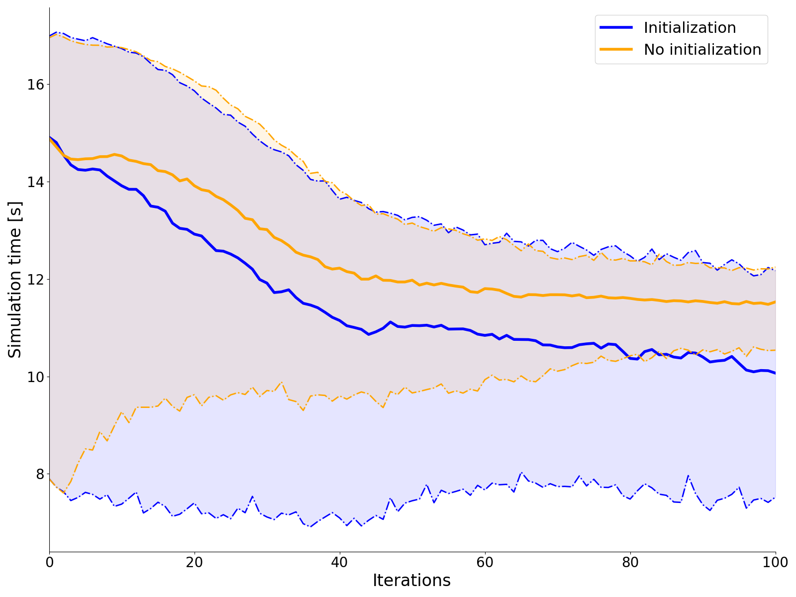
Figure 4: Computational improvements achieved through the use of simulation initialization. The comparison is conducted for the Simple Bay case, for identical sampling point locations. To ensure proper comparison the optimization seed remained consistent for both the initialization and no-initialization approaches. Colored segments represent simulation run times and are bounded by average maximum and minimum times. Dashed lines represent median maximum and minimum simulation times i.e. all simulation run times are expected to fall within this range. The cumulative impact and the overall reduction of the simulation time is evident. Initially, the improvement is negligible, but after 100 iterations can reach up to 20%.

5 Assessment of flow reconstruction accuracy depending on the number of sampling points

The accuracy of the flow field reconstruction depends not only on the number of sampling points, but also on the location of these points within the domain. A larger number of sampling points means more information for the optimization algorithm and therefore, typically, stable convergence and accurate results. However, if the locations of the sampling points are very close to each other, they effectively provide the same information about the velocity field, hence the number of effective sampling points is lower. To determine how many sampling points provide useful information, an effective number of sampling points $\eta$ is introduced.

For each sampling point, we decided to estimate the area of influence using the two-dimensional Gaussian function. The impact of sampling point $\mathbf{s}_{i}$ to its surroundings is characterized with

$$\phi_{i}(\mathbf{x})=\frac{1}{2\pi\sigma^{2}}\exp\left(-\frac{\left({\mathbf{x}}-{\mathbf{s}_{i}}\right)\cdot\left({\mathbf{x}}-{\mathbf{s}_{i}}\right)}{2\sigma^{2}}\right)$$ (14)

where $\sigma$ is standard deviation and $(\cdot)$ is a dot product. The scaling $\frac{1}{2\pi\sigma^{2}}$ ensures the volume under the Gaussian function is always equal to 1, regardless of $\sigma$.

Our goal is to cover the domain with $n_{SP}$ sampling points where, in ideal case, each covers the circle of a radius equal to three standard deviations (99.7% of the volume under $\phi$ is within three standard deviations from the sampling location $\mathbf{s}$). Considering the influence of all sampling points is equal, i.e. $\sigma$ is the same for all $i$, we can determine $\sigma$ from

$$9\sigma^{2}\cdot\pi\cdot n_{SP}=|\Omega|$$ (15)

where $|\Omega|$ is the area of the domain $\Omega$.

Now, when locations of sampling points and standard deviation $\sigma$ are known, we can calculate Gaussian function $\phi_{g}(x,y)$ around every sampling point in the domain. Consequently, if these points are close to each other, their influence will overlap. In order to calculate an effective influence, a maximum value of $\phi$ is taken. Finally, an effective number of sampling points $\eta$ is calculated as:

$$\eta=\int_{\Omega}\max(\phi_{1},...,\phi_{n_{SP}})\,d{\mathbf{x}}$$ (16)

where it is expected for resulting $\eta$ to be a positive real number to be less than number of sampling points ($0<\eta\leq n_{SP}$, for ideally distributed sampling points $\eta=n_{SP}$). Visual representation of $\eta$ can be seen in Figure 5.

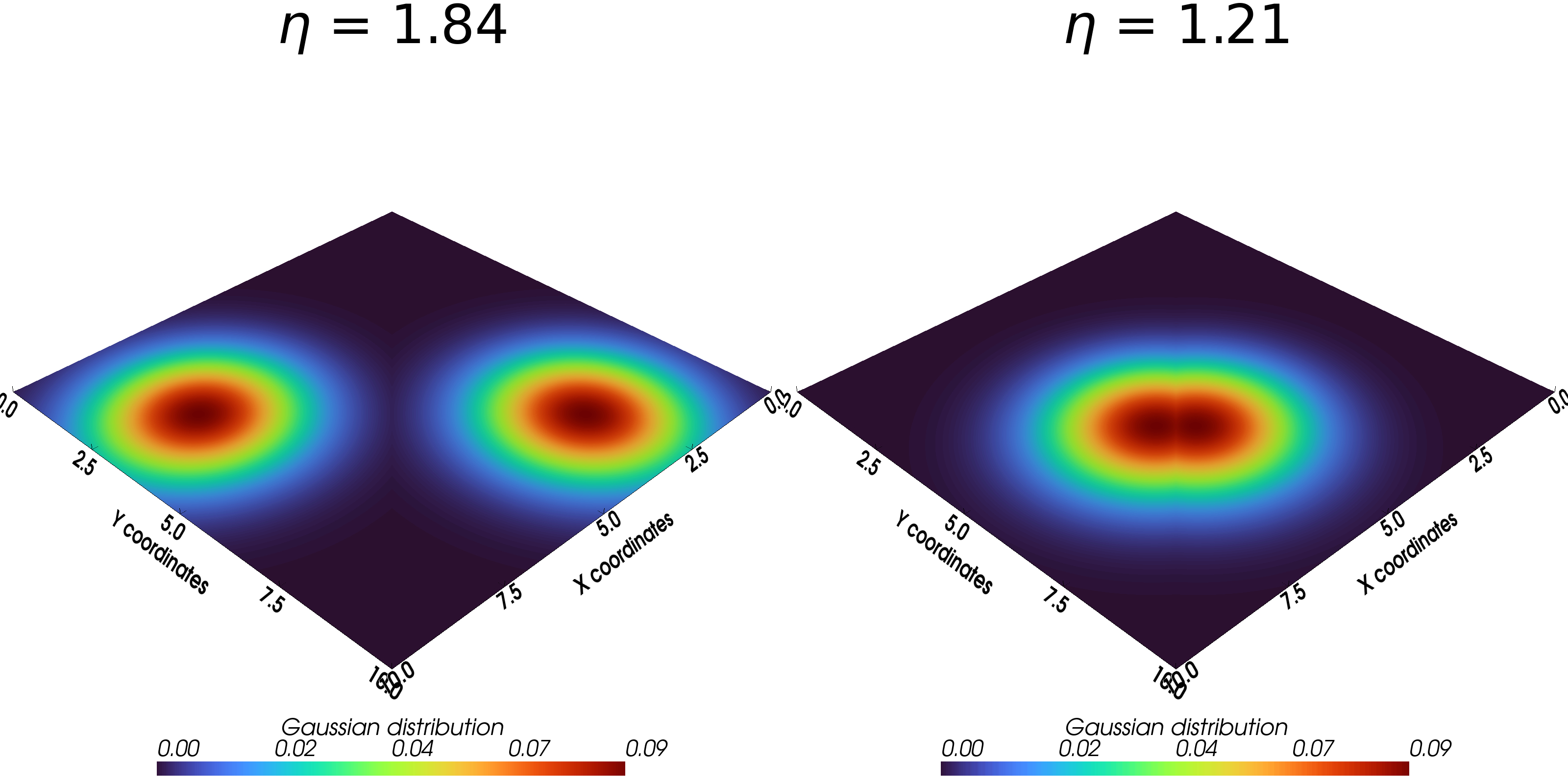
Figure 5: The sampling points on the left are distant enough and hence are able to provide unique information about different parts of the domain. In this case, $\eta$ is smaller than n because the domain is rectangular and the corners of the domain cannot be reached using the Gaussian distribution. The sampling points on the right are close to each other and, as shown, zones overlap, which means that sampling points partially provide the same information and therefore $\eta$ is much smaller than n.

To determine the impact of $\eta$ on the flow reconstruction results, 100 optimization runs were conducted for 1-20 sampling points which were randomly distributed across the domain. The results can be seen in Figure 6. As expected, the results are not reliable with a small number of sampling points (orange). As the number of sampling points increases, this behavior changes. The orange area does not represent an unsuccessful optimization, but rather a case where the number of sampling points is not sufficient to fully reconstruct the flow. The observed trend of the expansion of the green area suggests that the reconstruction of the flow field becomes more accurate as the number of sampling points increases.

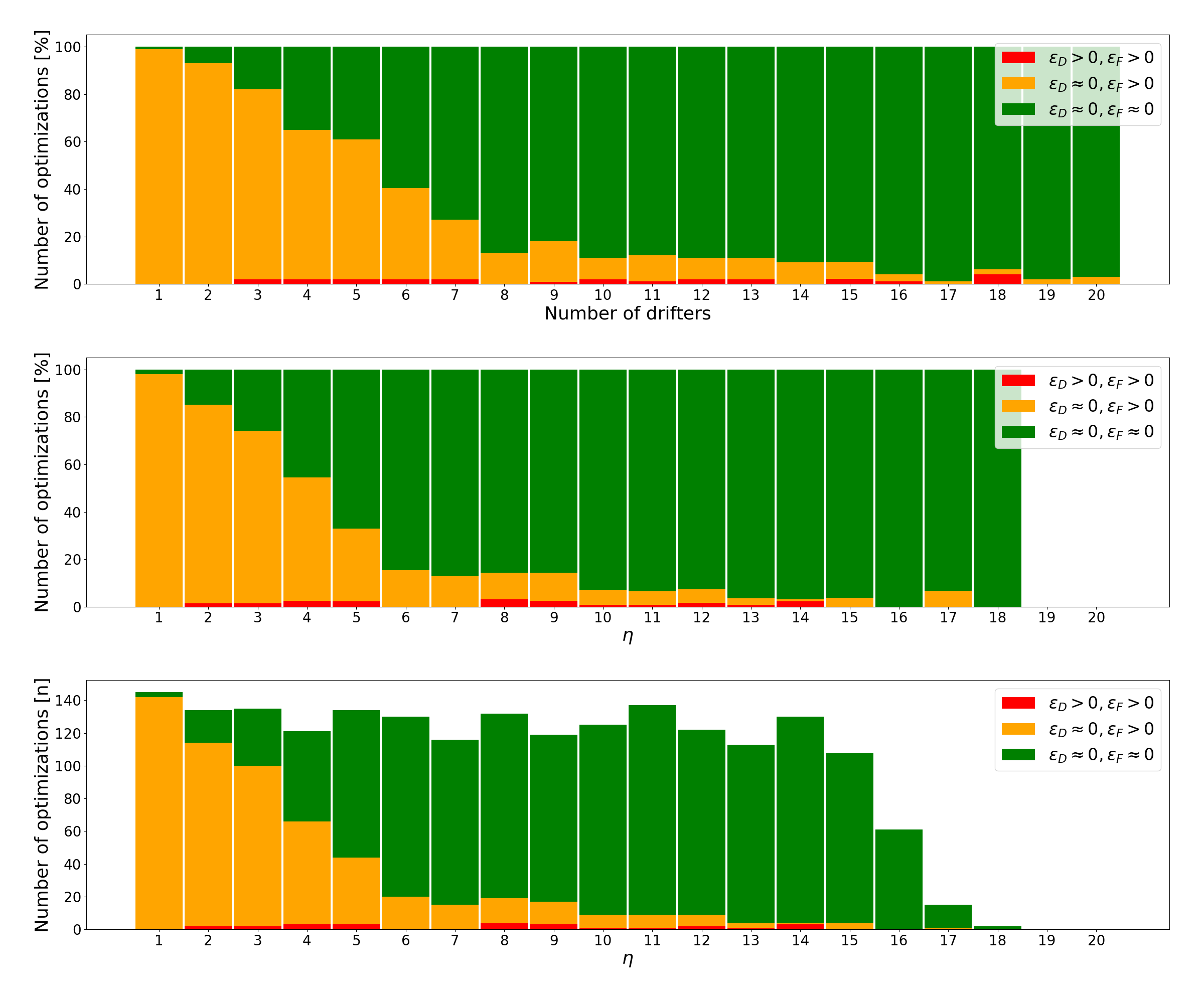
Figure 6: The range of potential scenarios resulting from 100 optimizations for each configuration of 1-20 sampling points randomly positioned in the domain. When the number of sampling points is small (e.g. 1-3), the drifter error threshold is reached, but the field reconstruction error $\epsilon$_f is significant (orange). As the number of sampling points increases, more data is available to the optimization algorithm, which leads to a better field reconstruction (green). This becomes even clearer in the second subplot, which shows the effective number of sampling points. Here, the orange area disappears completely, as more unique data is available to reconstruct the entire flow. The final plot shows the distribution of optimizations over the different effective sampling points numbers, demonstrating the correlation between the effective number of sampling points and the optimization results.

Figure 7 summarizes possible scenarios of the optimization process, with a visual comparison of the different scenarios and the reference flow. The figure confirms our hypothesis that the orange scenario ($\epsilon_{d}$ $\approx$ 0, $\epsilon_{f}$ > 0) as the number of drifters increases will eventually transition into the green area ($\epsilon_{d}$ $\approx$ 0, $\epsilon_{f}$ $\approx$ 0). On the other hand, the red scenario ($\epsilon_{d}$ > 0, $\epsilon_{f}$ > 0) corresponds to an insufficiently resolved problem where increasing the number of drifters may not improve the solution. The grey scenario($\epsilon_{d}$ > 0, $\epsilon_{f}$ $\approx$ 0) provides a flow field that is similar to the reference flow, with slight variations in the velocities of the sampling points. The placement of the drifters also plays an important role, i.e. it is possible to reconstruct the flow with a smaller number of drifters if they are strategically placed.

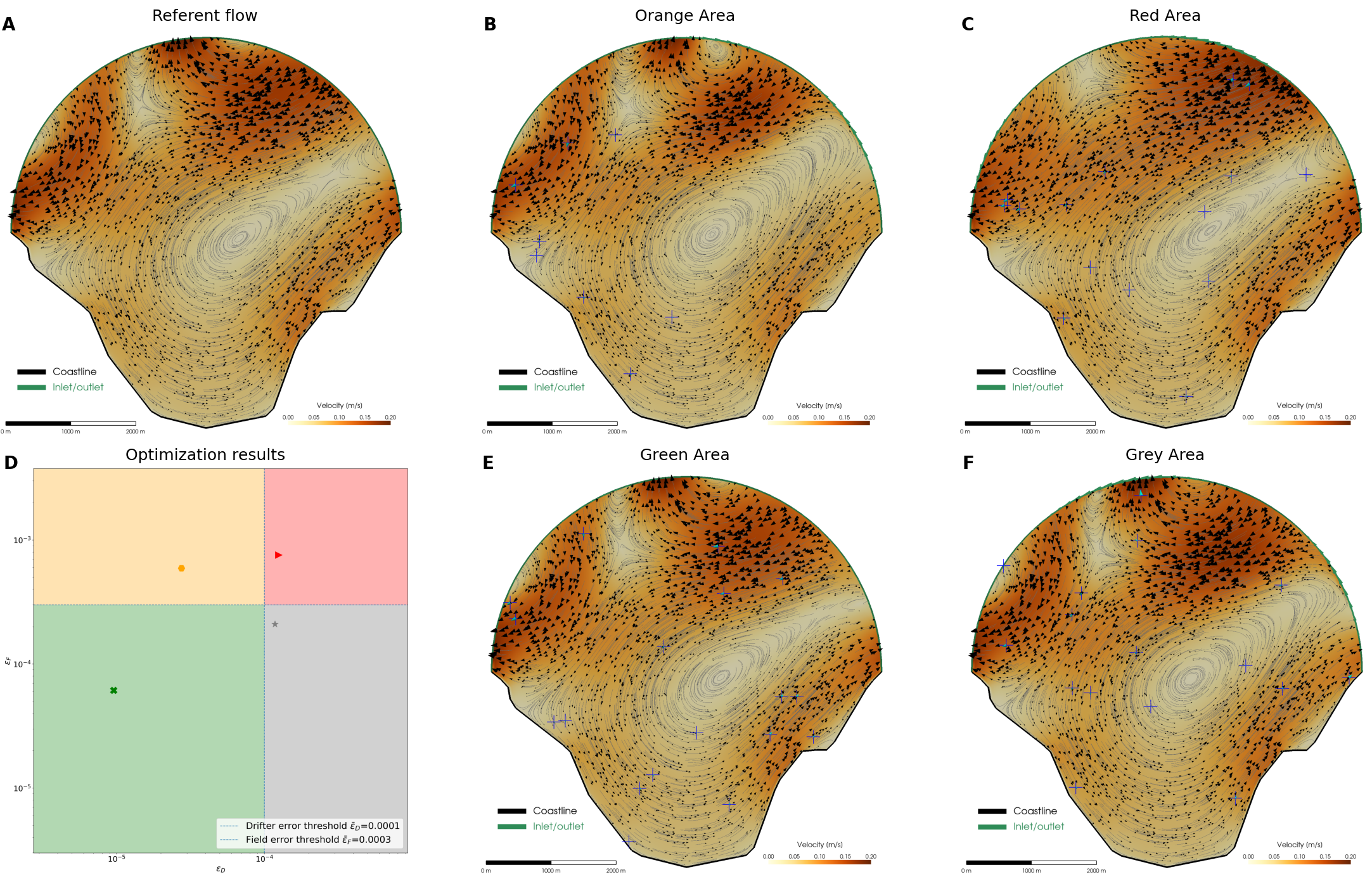
Figure 7: The flow field can be reconstructed in different ways depending on the placement of the sampling points and the threshold used to determine if the reconstruction is successful. (A) The reference case has two dominant flows in the northern and western parts of the domain, with a main vortex and a circular movement near the coastline. (B) 15 sampling points were used in this scenario, but only the main vortex is captured, with the flow in the northern part of the domain deviating significantly. This suggests that the optimization process did not have enough information in key regions. (C) With 7 sampling points, it is possible to accurately calculate the velocities at the sampling points locations, but the desired threshold for the entire field is not achieved. The strategic placement of additional sampling points could prompt the optimization to move toward the green area. (D) Displays the placement of optimization results within the scenario area. Adjusting the threshold for drifter error and field error could position these results differently, but through our investigation, we concluded that the threshold presented in the figure is most suitable for flow reconstruction. (E) Represents the green area scenario with 18 sampling points, where both drifter error and field error satisfy the desired threshold, conclusively indicating the successful reconstruction of the flow. The measurement data supports this conclusion, and the visual representation of the reconstructed flow closely resembles the referent one. (F) Case with 16 sampling points where the desired threshold for field error is satisfied but not for the drifter error. These are rare cases, attributable to numerical errors, and are consistently near the threshold. While this area bears great similarity to the referent case, the measurements at the sampling points locations differ just enough to fall short of the prescribed threshold.

6 Validation

To validate our simulation-based optimization approach, we created three test cases in addition to the Simple bay test case. Each of these test cases possesses distinct features that set it apart from the others. The unique characteristics of each test case are detailed in Table 3.

Table 3: Characteristics of the validation test cases

Case characteristics	Open water	Gulf of Trieste	Vis
Test case type	Synthetic	Realistic	Realistic
Domain area [$km^{2}$]	28.3	498.94	2273.9
Number of boundaries	1	1	5
Total boundary length [$km$]	125.65	20.52	120.97
Coastline length [$km$]	-	86.64	197.61
Number of boundary control points	12	5	14	-
Max velocity in the domain [$m/s$]	0.3	0.2	0.3.5
Presence of coastline/islands	No coastline	Coastline	Coastline and islands
Number of cells	9600	8262	12856
Average cell size [$m$]	361.75	245.74	412.41

For each test case, different optimization requirements and parameters (e.g. bounds and variables) are set. A comprehensive overview of these optimization characteristics is presented in Table 4.

Table 4: Optimization parameters for the validation test cases

Optimization characteristics	Open water	Gulf of Trieste		Vis
		Drifters	HF-radars	HF-radars
Number of sampling points $n_{SP}$	35	14	225	555
Number of objectives	2	2	2	2
Number of constraints	6	6	6	6
Number of optimization variables	20	6	6	28
Tangential velocity (bounds) [$m^{2}/s^{2}$]	-0.2 - 0.2	-0.5 - 0.5	-0.5 - 0.5	-0.5 - 0.5
Pressure (bounds) [$m^{2}/s^{2}$]	-0.025 - 0.025	-0.05 - 0.05	-0.05 - 0.05	-0.05 - 0.05
Average simulation time [$s$]	8.13	28.51	32.28	32.03
Average optimization time [$min$]	90.84	135.727	133.54	110.89

6.1 Open water

The Open water test case shown in Figure 8 represents a particular type of problem where the coastline is missing. This is a common problem when modeling and reconstructing e.g. ocean flow field. The entire boundary can vary, which makes the optimization process challenging. Despite these optimization challenges, this case is of great interest, applicable to small bays, and potentially even larger sea regions. Given the considerable size of this domain(20 $km$ radius), 30 sampling points were strategically positioned within the domain to reconstruct the surface flow. Like the Simple bay case, this scenario is synthetic, with $\mathbf{u}_{w}^{*}$ being 0. It can be seen from Figure 8 that the reconstructed flow has similar characteristics to the reference flow, although 4000 evaluations were required to achieve this through the optimization process.

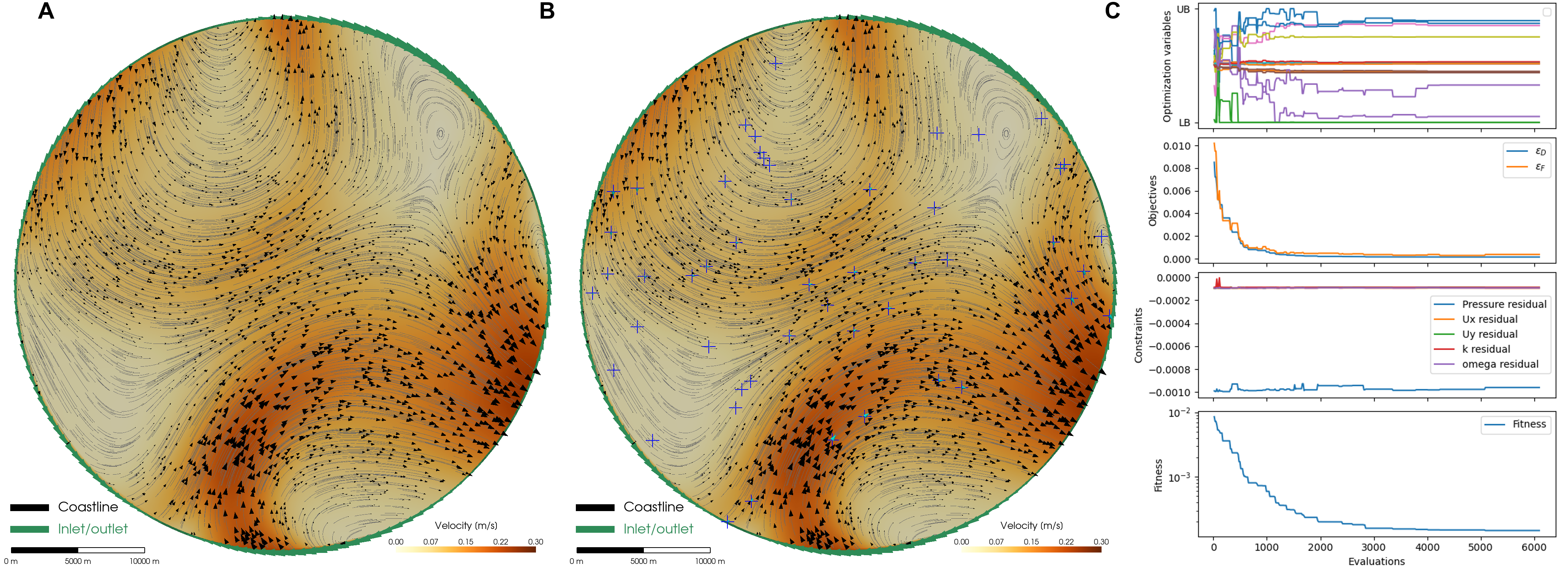
Figure 8: The figure depicts an Open water case, where the diameter of the domain is 40 km. Since the domain is very large, a total of 30 sampling points are used to reconstruct the flow. (A) The reference flow contains two main vortexes located in the northern and southern parts of the domain. The maximum velocity of 0.3 m/s is in line with expectations for a domain of this size. (B) The reconstructed flow with 30 sampling points, shown as blue crosses. On visual inspection of the field, the similarity to the reference flow is evident, with all vortexes and movements accurately captured. (C) Insight into the inlet/outlet boundary with 10 control points leading to 20 optimization variables. The first subplot on the right shows the variable values within the upper and lower limits defined by the optimization algorithm. The second subplot shows the alignment of field error and drifter error, whereby consistency is maintained throughout the entire optimization process. The third subplot shows that the pressure constraint is at its highest, but successfully follows the limits defined by the optimization algorithm. The fitness plot shows an initial steep drop within the first 1000 evaluations, followed by a gradual descent requiring approximately 4000 evaluations to achieve the target fitness.

6.2 Gulf of Trieste

The Gulf of Trieste, situated in the northernmost part of the Adriatic Sea, is a very shallow bay with an area of more than 500 square kilometers. Surface velocities in the same region were estimated by [30], where a combination of radar data, numerical modeling and acoustic Doppler current profilers (ADCPs) was used. The results of the study show that surface currents in the Gulf of Trieste exhibit considerable variability, with velocities ranging from less than 0.1 m/s to over 0.5 m/s. An overview of the Gulf and available measurement locations are given in Figure 9.

The validation of the Gulf of Trieste surface flow was carried out using data obtained as part of the TOSCA experiment in April 2012 [44]. The available drifter’s data indicate the presence of no more than 20 drifter locations with corresponding velocity magnitudes at the same time. Some drifters are closely positioned, leading to a reduced $\eta$ as depicted in Figure 10. Additionally, an analysis of the HF-radar data reveals that the flow vectors do not obey the principle of conservation of mass. This is evident from the fact that the velocity vectors are directed towards the coastline, as illustrated in Figure 11. This deviation can be attributed to the significant influence of the wind on the surface flow, resulting in directional changes that steer the vectors toward the coastline. The authors [30] themselves acknowledged that local conditions have a significant influence on surface velocities, which prompted us to include wind velocity in our evaluation function. The evaluation function extracts the velocities at the drifter locations and simultaneously integrates a wind velocity into the velocity vectors spanning the entire domain in x and y directions. As a result, the mass flux remains consistent, but the vectors tend to align directly with the coastline, providing a more realistic representation of the data.

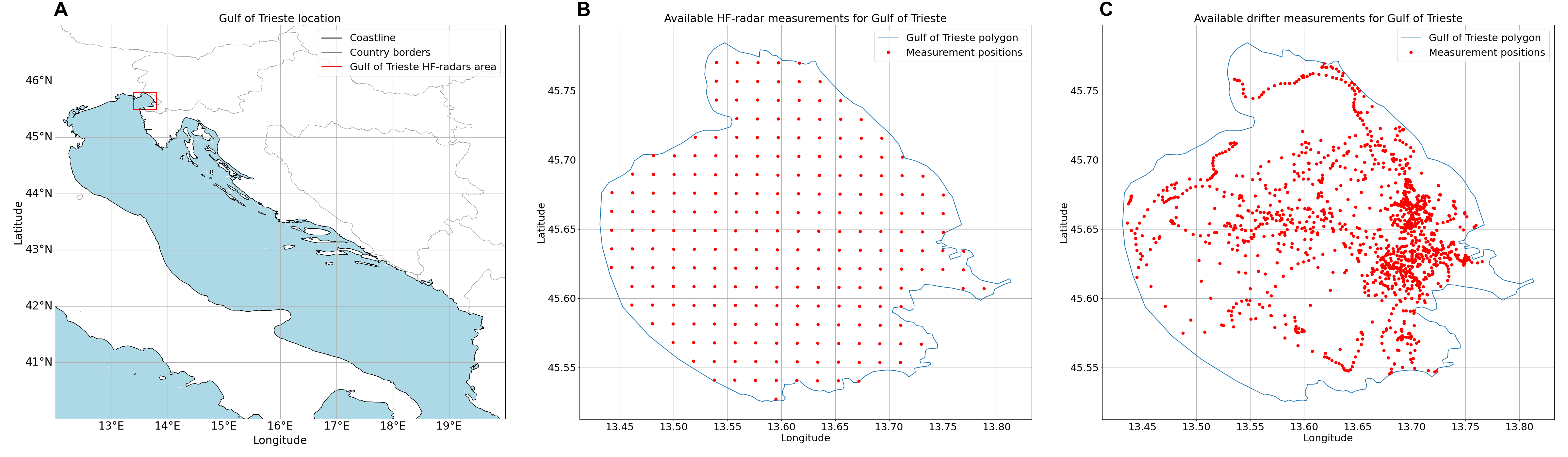
Figure 9: Figures show the Gulf of Trieste location in the Adriatic Sea and locations of available data based on drifter deployment and HF-radars. (A) Gulf of Trieste in the northern part of the Adriatic Sea where its area is approximately 550 square kilometers (B) 225 available HF-radar data locations within the domain of the Gulf of Trieste for April 2012, (C) Location of 44 drifters released within the domain of the Gulf of Trieste from 23rd April 2012 to 4th May 2012.

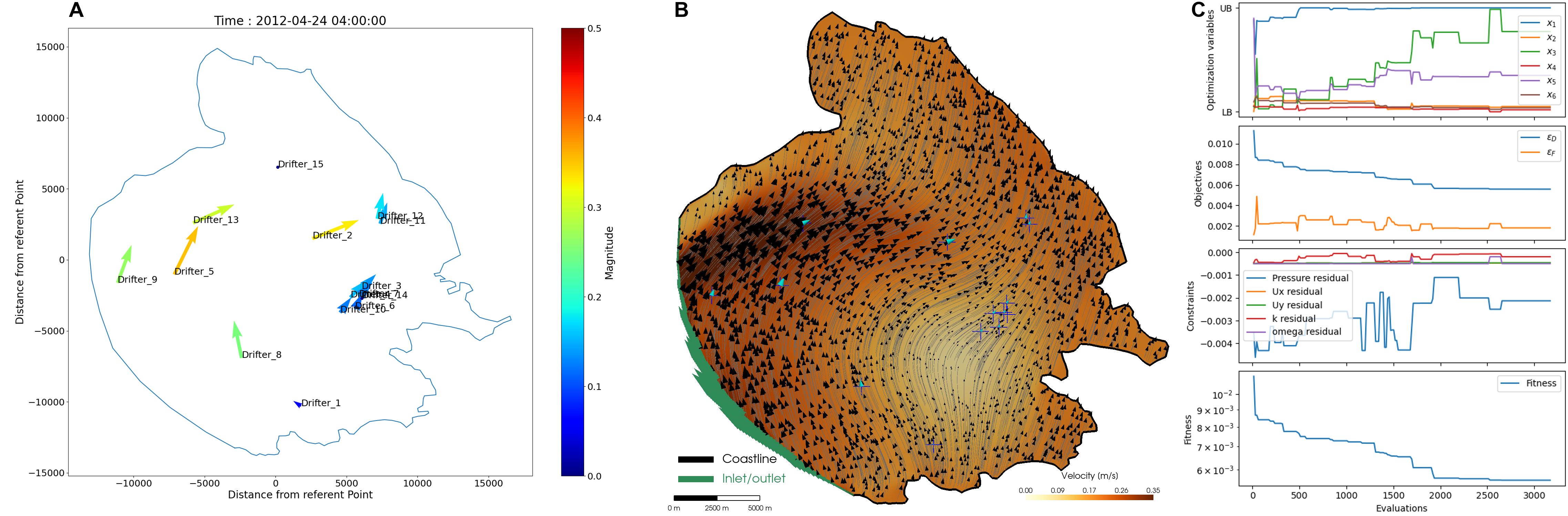
Figure 10: Figures show surface flow reconstruction results based on drifter measurements at 4 am on April 24th, 2012: (A) Displays the 15 available drifter locations and the corresponding velocity magnitudes at the specified time. Notably, some drifters are closely positioned, resulting in an effective number of sampling points $\eta$ of 9.59. The velocity magnitudes observed are below 0.4 m/s. (B) Illustrates the reconstructed surface flow from measurements obtained from the 15 available drifters, incorporating wind velocity where $\mathbf{u}_{w}^{*}=[5.88e^{-2},1.72e^{-1}]$ to capture the actual flow dynamics. (C) For this realistic case, only three control points were strategically placed, equating to six optimization variables. This decision was made due to the absence of vortexes in the flow, with a dominant flow observed from the southern to the northern part of the domain. Additional control points would only complicate the optimization process. Since only 15 drifters were available for this specific time, one drifter was utilized to track field error, resulting in a noticeable gap between drifter error and field error in the second subplot. The third subplot presents the changes in constraints throughout the optimization process. It is observed that pressure oscillates more than other parameters, but remains within the allowed range. The fitness plot indicates that the optimization did not reach the set threshold. However, the obtained results are considered highly satisfying.

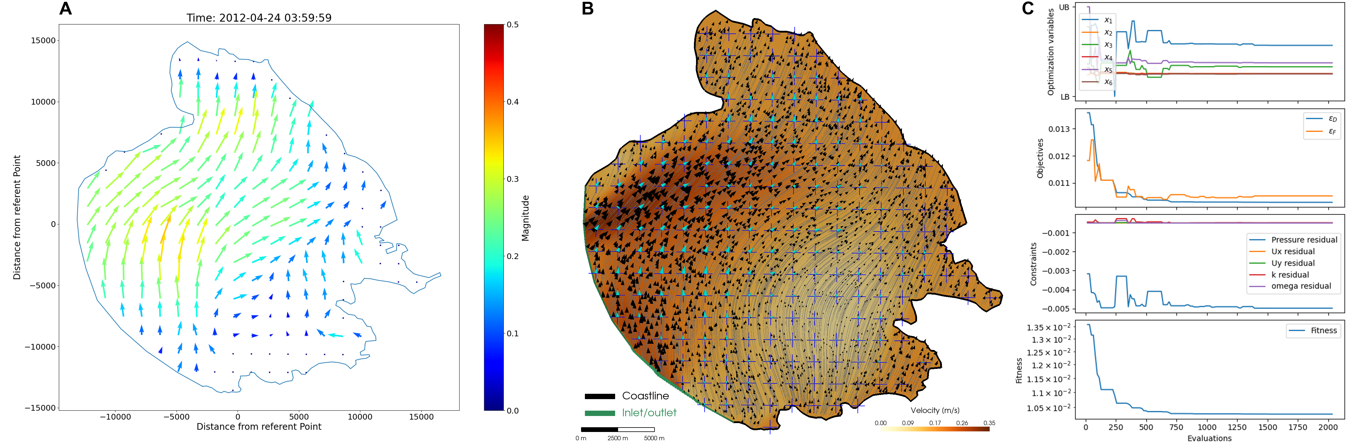
Figure 11: Figures shows surface flow reconstruction results based on HF-radar measurements at 4 am on April 24th, 2012: (A) Presents the 225 HF-radar data locations, showcasing the corresponding velocity magnitudes at the specified time. We used the same time as in 10 in order to compare the reconstructed flow obtained from both drifters and HF-radar measurements. (B) The reconstructed surface flow employing wind velocity where $\mathbf{u}_{w}^{*}=[6.17e^{-2},1.42e^{-1}]$. Cyan arrows represent optimized velocity vectors that are aligned with HF-radar measurements, providing a visual representation of the accuracy of the reconstruction. (C) Following a similar approach as demonstrated in Figure 10, only three control points were strategically placed, resulting in six optimization variables, as reflected in the first subplot. Similar to the drifter scenario, only one HF-radar measurement was used to track field error. Due to the significantly larger number of scatter measurements (224 v 14), there is no gap between the objectives. The third subplot exhibits oscillations in pressure residual for the first 700 evaluations, which then stabilize towards the end of the optimization. The fitness plot indicates a steep decline in the initial 500 evaluations, followed by fine-tuning until the completion of the optimization process. While the optimization did not achieve the desired threshold, the results are deemed highly satisfying, especially when visually comparing the referent flow to the optimized one.

The difference between the drifter data and the HF-radar data can be clearly seen in Figure 12. This difference is mainly due to the way in which drifters operate; they are deployed on the surface, which makes them very dependent on external factors such as wind and tides. HF-radar, on the other hand, uses radio waves to measure the speed and direction of surface currents. The radar emits high-frequency radio waves that bounce off the sea surface. By analyzing the frequency shifts of the reflected waves, the radar can determine the movement of the water. The reconstructed flow, obtained from both drifters and HF-radar (utilized as sampling points in this instance), exhibits a notably similar pattern with slight variations. Nevertheless, the main flow, magnitudes and direction confirm the efficiency of our modeling approach that compensates for the wind, especially when a sufficient number of drifters are used to cover a substantial part of the domain. This means that any assessment without the inclusion of wind velocity would be impractical.

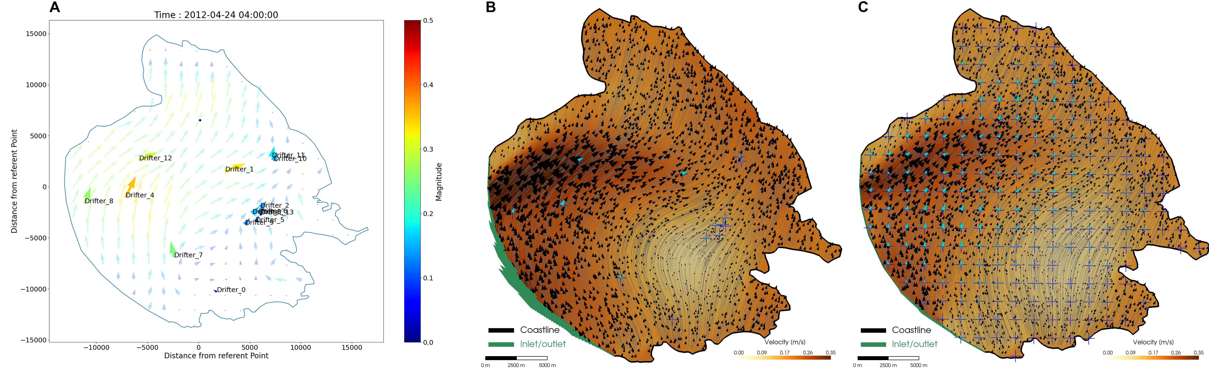
Figure 12: This figure portrays variations in flow reconstruction results obtained from both HF-radar and drifters at the exact time on April 24th, 2012: (A) Combines HF-radar data locations (in the background) and drifter locations, showcasing the corresponding velocity magnitudes at 4 am on April 24th, 2012. Although they measure the same data, disparities in magnitude and directions are noticeable, implying that the reconstructed flow might exhibit slight differences. (B) Illustrates the reconstructed surface flow based on 15 available drifter data, incorporating wind velocity to enhance accuracy. (C) Presents the reconstructed surface flow based on 225 HF-radar data, also incorporating wind velocity. The primary flow patterns appear quite similar between the two data sources, with the drifter data introducing a slightly broader circulation compared to the HF-radar data.

6.3 Vis case

The area around the island of Vis lies in the central part of the Adriatic, close to the Croatian coast, and covers more than 2200 square kilometers. An important aspect of this case is the presence of islands within the domain, together with several inlets and outlets, making it a comprehensive test scenario covering all possible problem variants. The data for this case were obtained from the Institute of Oceanography and Fisheries [45] provided HF data from October 2019, taken with two HF-radars that are currently inactive. We opted for a larger area than the locations of the HF-radar data as we wanted to map the evolution of the flow as it reaches the region covered by the available HF-radar data as shown in Figure 13.

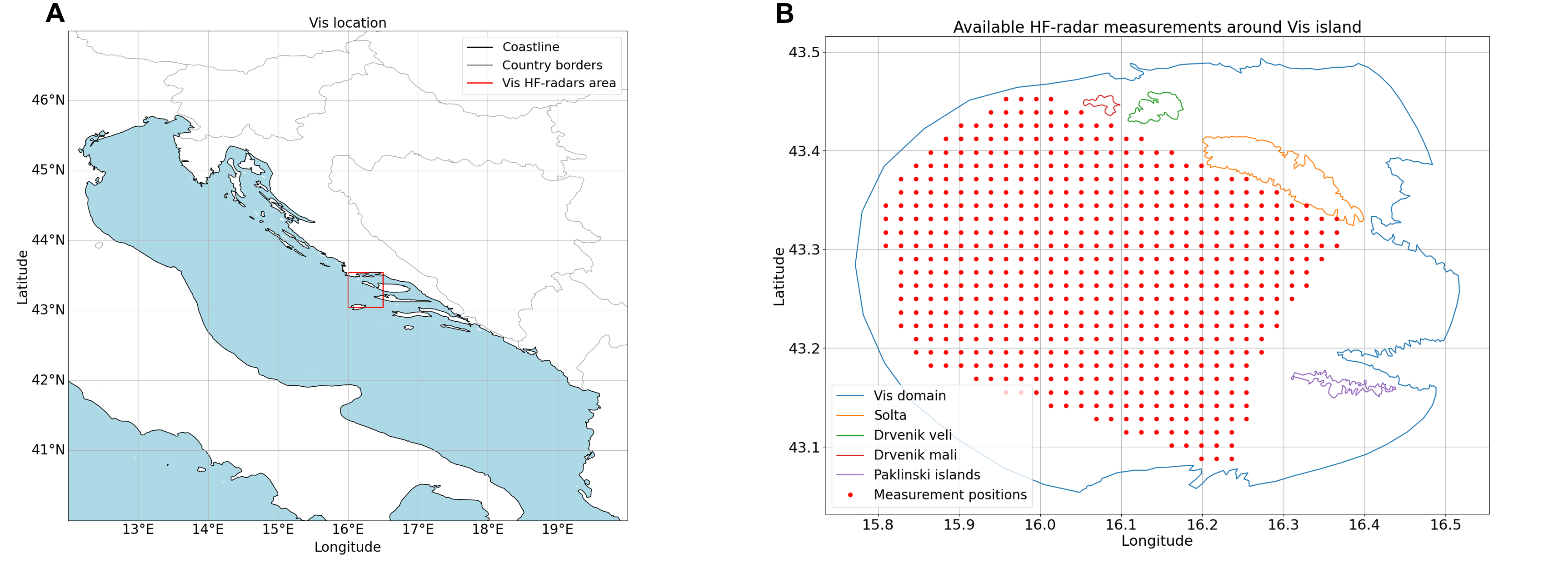
Figure 13: Figures show the location of the domain around Vis island in the Adriatic Sea and locations of available HF-radar data: (A) Domain around Vis island in the central part of Adriatic Sea with more than 2200 square kilometers. (B) 555 HF-radar data values within the domain around Vis island including 4 islands and a coastline.

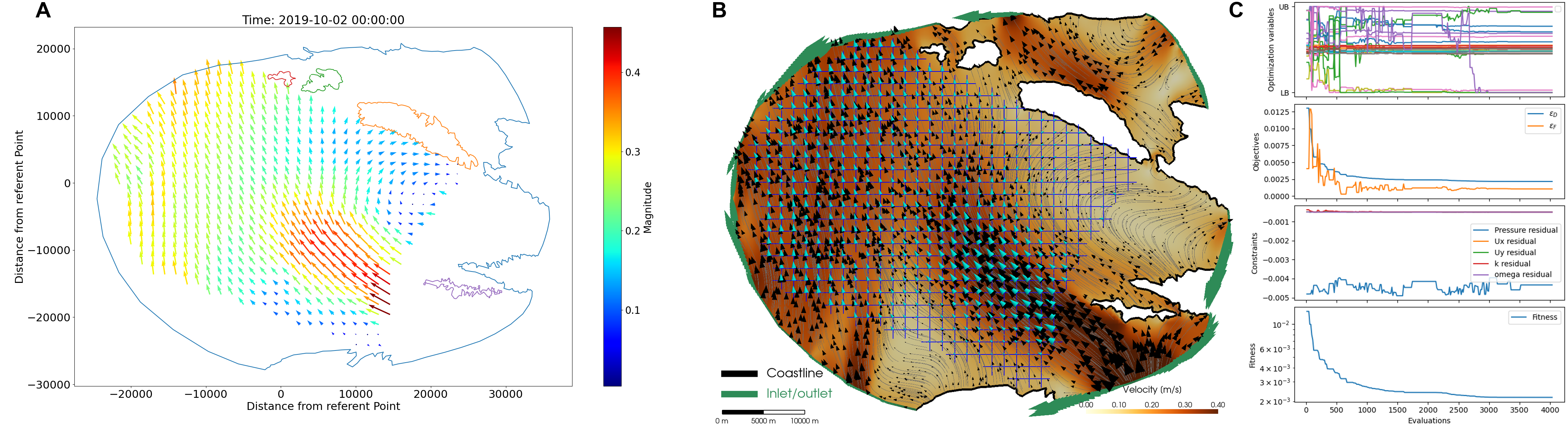
Figure 14: Figures show surface flow reconstruction results based on HF-radar measurements at midnight on October 2nd, 2019. (A) HF-radar data locations with corresponding velocity magnitudes at specified time. In this case, a larger area than the available HF-radar measurements was considered to allow the flow to develop as it reaches the measurement positions. (B) Illustrates the reconstructed surface flow, where optimized velocity vectors, represented as cyan arrows, closely match the HF-measurements. This alignment signifies the successful reconstruction of the flow dynamics. (C) This particular case represents a very complex scenario with four islands and five different inlet/outlet boundaries. To address this complexity, 14 control points were strategically placed on the boundaries, resulting in 28 optimization variables which is the highest number. One of the HF-measurement locations was again utilized to track field error. The second subplot reveals a gap between objectives, showcasing a smaller error at this specific position compared to the error of all measurement positions. Similar to other cases, pressure residual exhibits oscillations, all within the desired range. The fitness plot displays a gradual decline from the start to the end of optimization, concluding at 4000 evaluations. Despite not reaching the desired threshold, the resemblance between HF-radar measurements and the reconstructed flow is significant.

According to Figure 14, the reconstructed flow pattern mirrors the flow pattern of the measurements obtained from HF-radars, which validates the effectiveness of our simulation-based optimization approach in reconstructing the surface flow. Similar to the case of the Gulf of Trieste, we incorporated a wind velocity where $\mathbf{u}_{w}^{*}=[-7.35e^{-2},1.12e^{-1}]$ to account for atypical flows flowing directly onto the coast and around the islands. By integrating this feature, we demonstrated that our modeling approach can effectively capture real-world data and thus provide a fast approximation of the surface flow.

7 Limitations and discussion

The simulation-optimization methodology does not take into account factors such as wind, tides, and temperature fluctuations. This is a deliberate decision to make the model simpler and thus computationally more efficient. The dynamics of strong winds that change the direction of flow and the complicated interplay of changing tides and temperature fluctuations present challenges that are overlooked in the pursuit of calculation speed.

From a computational perspective, the use of coarse numerical meshes, as proposed, can be advantageous in terms of efficiency, which can be particularly useful in time-constrained search and rescue operations. However, certain disadvantages and limitations must be taken into account. The proposed simplification may limit the ability of the surrogate to capture the complexity of a realistic flow field. Nevertheless, it is suitable for fast approximations given that the approximated surrogate velocity field replicates real flows within an acceptable margin. Another time-saving feature is the simulation initialization approach, which can provide significant speedup, especially in more complex domains. However, one challenge associated with the initialization approach is its potential to steer the optimization in the wrong direction, as all cases inherit the internal field from the currently best found flow.

Problems with field reconstruction arise when there are not enough drifters, as it is difficult to calculate field error and decide which of the four optimization outcomes our results match. This is especially true if the drifters are confined to a small area, making it impossible to accurately reconstruct the flow in a larger domain. However, this issue can be addressed by strategically placing drifters and using an effective number of drifters calculation to assess domain coverage and the reliability of the reconstructed flow. Fortunately, if HF-radar measurements are available for a certain area, they can be used to improve accuracy as there are usually a large number of measurements. This demonstrates the versatility of our methodology with multiple data sources.

Overall, the model’s strengths and limitations highlight the importance of achieving a careful balance between speed and accuracy when aiming for effective flow approximation, especially in situations where time is of the essence.

8 Conclusion

Current approaches to surface flow reconstruction, while effective in certain aspects, often lack detailed insights into the specific characteristics, behavior, and attributes defining the physical properties of a flow field. Furthermore, they can often be complex and computationally demanding, thus their applicability in real-case time-constrained scenarios is limited. In response to this limitation, a simulation-based optimization approach that utilizes a simplified two-dimensional surrogate flow model is introduced. The methodology adjusts boundary conditions in order to align the computed velocity field with scattered measurements. The intentional exclusion of some influential phenomena, such as wind, waves, changing tides, and temperature variations, prioritizes speed in our surrogate model.

From a computational perspective, the proposed use of coarse numerical meshes in our methodology improves efficiency, especially in time-sensitive search and rescue operations. However, it is important to acknowledge the potential inaccuracies in capturing the complexity of realistic flow fields is crucial. The simulation initialization approach, while providing substantial acceleration, presents challenges in the optimization process, particularly in scenarios where flow dynamics are not constrained by the coastline as it is the case in Open water scenario. Despite the simplifications, our simulation-based optimization approach brings distinct advantages over traditional methods. It generally requires a smaller number of drifters, reducing the cost and time for data collection, and provides more accurate velocity field obtainable for entire simulated domain, even for areas with no sampling points nearby. Potential field reconstruction issues due to insufficient drifters can be addressed through strategic drifter placement and effective calculations of the number of drifters. Additionally, the incorporation of HF-radar measurements, where available, enhances accuracy, showcasing the versatility of our methodology in leveraging multiple data sources.

The inclusion of surrogate model in our simulation-based optimization approach offers a promising alternative to conventional methods, demonstrating its potential to enhance accuracy and efficiency in fluid mechanics, oceanography, and environmental engineering applications. While challenges exist, the adaptability and advantages of our methodology position it as a valuable tool for advancing research and practical applications in the field.

Data availability

All parameters for reproducing the study are presented in the manuscript. The data needed to reproduce the presented method and cases are available on The Open Science Framework repository: https://osf.io/pdtbh/. The Python code needed to reproduce this research is available upon request.

References

- [1] L. Sombardier, P. P. Niiler, Global surface circulation measured by lagrangian drifters, Sea Technology;(United States) 35 (10) (1994).
- [2] J. C. Ohlmann, P. P. Niiler, Circulation over the continental shelf in the northern gulf of mexico, Progress in oceanography 64 (1) (2005) 45–81.
- [3] S. F. DiMarco, W. D. Nowlin, R. Reid, A statistical description of the velocity fields from upper ocean drifters in the gulf of mexico, Geophysical Monograph-American Geophysical Union 161 (2005) 101.
- [4] G. Lacorata, E. Aurell, A. Vulpiani, Drifter dispersion in the adriatic sea: Lagrangian data and chaotic model, Vol. 19, Copernicus GmbH, 2001, pp. 121–129.
- [5] P. Falco, A. Griffa, P.-M. Poulain, E. Zambianchi, Transport properties in the adriatic sea as deduced from drifter data, Journal of Physical Oceanography 30 (8) (2000) 2055–2071.
- [6] P.-M. Poulain, Adriatic sea surface circulation as derived from drifter data between 1990 and 1999, Journal of Marine Systems 29 (1-4) (2001) 3–32.
- [7] L. Ursella, P.-M. Poulain, R. P. Signell, Surface drifter derived circulation in the northern and middle adriatic sea: Response to wind regime and season, Journal of Geophysical Research: Oceans 111 (C3) (2006).
- [8] M. Toner, A. Kirwan Jr, B. Lipphardt, A. Poje, C. Jones, C. Grosch, Reconstructing basin-scale eulerian velocity fields from simulated drifter data, Journal of physical oceanography 31 (5) (2001) 1361–1376.
- [9] A. C. Haza, E. D’Asaro, H. Chang, S. Chen, M. Curcic, C. Guigand, H. Huntley, G. Jacobs, G. Novelli, T. Özgökmen, et al., Drogue-loss detection for surface drifters during the lagrangian submesoscale experiment (laser), Journal of atmospheric and oceanic technology 35 (4) (2018) 705–725.
- [10] F. Hernandez, P.-Y. Le Traon, R. Morrow, Mapping mesoscale variability of the azores current using topex/poseidon and ers 1 altimetry, together with hydrographic and lagrangian measurements, Journal of Geophysical Research: Oceans 100 (C12) (1995) 24995–25006.
- [11] A. Molcard, L. I. Piterbarg, A. Griffa, T. M. Özgökmen, A. J. Mariano, Assimilation of drifter observations for the reconstruction of the eulerian circulation field, Journal of Geophysical Research: Oceans 108 (C3) (2003).
- [12] D. B. Rao, D. J. Schwab, A method of objective analysis for currents in a lake with application to lake ontario, Journal of Physical Oceanography 11 (5) (1981) 739–750.
- [13] V. Eremeev, L. Ivanov, A. Kirwan Jr, Reconstruction of oceanic flow characteristics from quasi-lagrangian data: 1. approach and mathematical methods, Journal of Geophysical Research: Oceans 97 (C6) (1992) 9733–9742.
- [14] K. Cho, R. O. Reid, W. D. Nowlin Jr, Objectively mapped stream function fields on the texas-louisiana shelf based on 32 months of moored current meter data, Journal of Geophysical Research: Oceans 103 (C5) (1998) 10377–10390.
- [15] R. C. Gonçalves, M. Iskandarani, T. Özgökmen, W. C. Thacker, Reconstruction of submesoscale velocity field from surface drifters, Journal of Physical Oceanography 49 (4) (2019) 941–958.
- [16] E. D’asaro, C. Lee, L. Rainville, R. Harcourt, L. Thomas, Enhanced turbulence and energy dissipation at ocean fronts, science 332 (6027) (2011) 318–322.
- [17] G. Novelli, C. M. Guigand, C. Cousin, E. H. Ryan, N. J. Laxague, H. Dai, B. K. Haus, T. M. Özgökmen, A biodegradable surface drifter for ocean sampling on a massive scale, Journal of Atmospheric and Oceanic Technology 34 (11) (2017) 2509–2532.
- [18] J. L. Callaham, K. Maeda, S. L. Brunton, Robust flow reconstruction from limited measurements via sparse representation, Physical Review Fluids 4 (10) (2019) 103907.
- [19] J. Marmain, A. Molcard, P. Forget, A. Barth, Y. Ourmieres, Assimilation of hf radar surface currents to optimize forcing in the northwestern mediterranean sea, Nonlinear Processes in Geophysics 21 (3) (2014) 659–675.
- [20] D. Inazu, T. Higuchi, K. Nakamura, Optimization of boundary condition and physical parameter in an ocean tide model using an evolutionary algorithm, Theoretical and Applied Mechanics Japan 58 (2010) 101–112.
- [21] S. Ghalambaz, M. Abbaszadeh, I. Sadrehaghighi, O. Younis, M. Ghalambaz, M. Ghalambaz, A forty years scientometric investigation of artificial intelligence for fluid-flow and heat-transfer (aifh) during 1982 and 2022, Engineering Applications of Artificial Intelligence 127 (2024) 107334.
- [22] N. O. Aksamit, T. Sapsis, G. Haller, Machine-learning mesoscale and submesoscale surface dynamics from lagrangian ocean drifter trajectories, Journal of Physical Oceanography 50 (5) (2020).
- [23] M. D. Grossi, M. Kubat, T. M. Özgökmen, Predicting particle trajectories in oceanic flows using artificial neural networks, Ocean Modelling 156 (2020) 101707.
- [24] J. Jiang, G. Li, Y. Jiang, L. Zhang, X. Deng, Transcfd: A transformer-based decoder for flow field prediction, Engineering Applications of Artificial Intelligence 123 (2023) 106340.
- [25] S. Hu, M. Liu, S. Zhang, S. Dong, R. Zheng, Physics-informed neural network combined with characteristic-based split for solving navier–stokes equations, Engineering Applications of Artificial Intelligence 128 (2024) 107453.
- [26] M. A. Kazemi, M. Pa, M. N. Uddin, M. Rezakazemi, Adaptive neuro-fuzzy inference system based data interpolation for particle image velocimetry in fluid flow applications, Engineering Applications of Artificial Intelligence 119 (2023) 105723.
- [27] M. D. Gunzburger, Finite element methods for viscous incompressible flows: a guide to theory, practice, and algorithms, Elsevier, 2012.
- [28] P.-L. Lions, Mathematical Topics in Fluid Mechanics: Volume 2: Compressible Models, Vol. 2, Oxford Lecture Mathematics and, 1996.
- [29] M. Kronbichler, Numerical methods for the navier–stokes equations applied to turbulent flow and to multi-phase flow, Ph.D. thesis, Uppsala University (2009).
- [30] S. Cosoli, M. Ličer, M. Vodopivec, V. Malačič, Surface circulation in the gulf of trieste (northern adriatic sea) from radar, model, and adcp comparisons, Journal of Geophysical Research: Oceans 118 (11) (2013) 6183–6200.
- [31] G. Notarstefano, P.-M. Poulain, E. Mauri, Estimation of surface currents in the adriatic sea from sequential infrared satellite images, Journal of Atmospheric and Oceanic Technology 25 (2) (2008) 271–285.
- [32] R. Bolaños, J. V. T. Sørensen, A. Benetazzo, S. Carniel, M. Sclavo, Modelling ocean currents in the northern adriatic sea, Continental Shelf Research 87 (2014) 54–72.
-
[33]
J. Ferziger, M. Peric,
Computational Methods
for Fluid Dynamics, Springer Berlin Heidelberg, 2012.
URL https://books.google.hr/books?id=BZnvCAAAQBAJ - [34] F. R. Menter, Improved two-equation k-omega turbulence models for aerodynamic flows, Tech. rep. (1992).
- [35] F. Juretic, cfmesh user guide, Creative Fields, Ltd 1 (2015).
- [36] T. O. Foundation, OpenFOAM User Guide, howpublished = "http://aiweb.techfak.uni-bielefeld.de/content/bworld-robot-control-software/", year = 2016, note = "[online; accessed 04-april-2023]".
- [37] S. V. Patankar, D. B. Spalding, A calculation procedure for heat, mass and momentum transfer in three-dimensional parabolic flows, in: Numerical prediction of flow, heat transfer, turbulence and combustion, Elsevier, 1983, pp. 54–73.
- [38] P. Virtanen, R. Gommers, T. E. Oliphant, M. Haberland, T. Reddy, D. Cournapeau, E. Burovski, P. Peterson, W. Weckesser, J. Bright, et al., Scipy 1.0: fundamental algorithms for scientific computing in python, Nature methods 17 (3) (2020) 261–272.
-
[39]
S. Ivić, S. Družeta,
Indago: Python 3 module for
numerical optimization.
URL https://pypi.org/project/Indago/0.4.5/ - [40] J. Kennedy, R. Eberhart, Particle swarm optimization, in: Proceedings of ICNN’95-international conference on neural networks, Vol. 4, IEEE, 1995, pp. 1942–1948.
- [41] Y. Tan, Y. Zhu, Fireworks algorithm for optimization, in: Advances in Swarm Intelligence: First International Conference, ICSI 2010, Beijing, China, June 12-15, 2010, Proceedings, Part I 1, Springer, 2010, pp. 355–364.
- [42] D. Karaboga, et al., An idea based on honey bee swarm for numerical optimization, Tech. rep., Technical report-tr06, Erciyes university, engineering faculty, computer … (2005).
- [43] A. Mohammadi, F. Sheikholeslam, Intelligent optimization: Literature review and state-of-the-art algorithms (1965–2022), Engineering Applications of Artificial Intelligence 126 (2023) 106959.
-
[44]
M. G. Magaldi, C. Mantovani, S. Cosoli,
Current velocities measured by
HF radars in Gulf of Trieste - April 2012, This dataset was produced
thanks to the Tracking Oil Spills and Coastal Awareness (TOSCA) Network
project [grant number 2G-MED09-425], co-financed by the European Regional
Development Fund in the framework of the MED programme (Jun. 2019).
doi:10.5281/zenodo.3245409.
URL https://doi.org/10.5281/zenodo.3245409 - [45] I. of Oceanography, Fisheries, Physical Oceanography Laboratory, howpublished = "https://galijula.izor.hr/en/", year = 2023, note = "[online; accessed 19-october-2023]".