On the visualisation of the correlation matrix

Abstract

Extensions of earlier algorithms and enhanced visualization techniques for approximating a correlation matrix are presented. The visualization problems that result from using column or colum–and–row adjusted correlation matrices, which give numerically a better fit, are addressed. For visualization of a correlation matrix a weighted alternating least squares algorithm is used, with either a single scalar adjustment, or a column-only adjustment with symmetric factorization; these choices form a compromise between the numerical accuracy of the approximation and the comprehensibility of the obtained correlation biplots. Some illustrative examples are discussed.

Keywords: biplot; correlation tally stick; principal component analysis; weighted alternating least squares;

1 Introduction

The correlation matrix is of fundamental importance in many scientific studies that use multiple variables. The visualization of correlation structure is therefore of great interest. In a recent article (Graffelman & De Leeuw, 2023b), multivariate statistical methods for the visualization of the correlation matrix were reviewed, and a low-rank approximation with a scalar adjustment, obtained by a weighted alternating least squares algorithm was proposed. This was shown to improve the approximation of the correlation matrix in comparison with existing methods like principal component analysis (pca) in terms of the root mean squared error (rmse). The previous work (Graffelman & De Leeuw, 2023b) capitalized on simplicity and symmetry of the visualization. In this article, it is shown that approximations of the correlation matrix with lower rmse are possible, but that these come at the price of sacrificing either simplicity or symmetry or both. One thus has to seek a balance between the numerical exactness of the approximation on one hand, and the comprehensibility of the visualization on the other. Simplicity refers to using one single vector (or point) to represent each variable. Doubling the number of points per variable quite obviously gives more flexibility in approximating the correlation matrix, but comes at the price of more dense and less attractive visualizations. Symmetry refers to symmetry of the approximation, in the sense that projecting vector A onto B leads to the same approximation to the correlation as projecting B onto A. To make these principles clear, four biplots of the correlation matrix of the banknote data are shown in Figure 1; this data set consists of six size measurements (Top, Bottom, Length, Left, Right and Diagonal) on a sample of Swiss banknotes (Weisberg (2005), using counterfeits only). At this point, we do not worry about avoiding the fit of the diagonal of the correlation matrix, something that will be efficiently dealt with by the weigthed alternating least squares (wals) algorithm later. Figure 1A shows the ”crude” approximation to $\mathbf{R}$ obtained by pca. Its origin represents zero correlation for all variables. Figure 1B shows the biplot obtained after adjustment by a single scalar $\delta$, here taken to be the overall mean of the correlation matrix ($\delta=\mathbf{1}^{\prime}\mathbf{R}\mathbf{1}/p^{2}$), and represents $\mathbf{R}_{a}=\mathbf{R}-\delta\mathbf{J}$. Its origin represents correlation $r_{..}$ ($0.20$) for all variables, where we use the dot subindex to indicate averaging over the corresponding index. Figure 1C gives the biplot after single-centring or adjustment by column means ($\mathbf{R}_{c}=\mathbf{H}\mathbf{R}$, with idempotent centring matrix $\mathbf{H}=\mathbf{I}-(1/p)\mathbf{1}\mathbf{1}^{\prime}$); its origin represents, for the $i$th variable, $r_{i.}$. Finally, Figure 1D shows the biplot after after double-centring or adjustment by both row and column means ($\mathbf{R}_{dc}=\mathbf{H}\mathbf{R}\mathbf{H}$) where the $i$th variable has origin $r_{i.}+r_{.j}-r_{..}$. In each case, the biplot is obtained by the singular value decomposition (svd; Eckart & Young (1936)) of the corresponding adjusted correlation matrix.

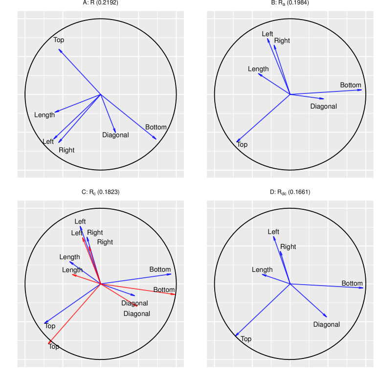
Figure 1: Visualizations of the correlation matrix obtained by standard pca (panel A), overall centering (panel B), column centering (panel C) and double centering (panel D).

The rmse of the approximation is seen to decrease as we successively use $0,1,p$ and $2p$ adjustment parameters. The pca biplot respects simplicity and symmetry, though it gives the worst approximation. Scalar adjustment retains simplicity and symmetry, and improves the approximation. Column adjustment destroys both simplicity and symmetry, but improves the approximation. In the corresponding biplot (Fig. 1C), correlations are approximated by scalar products between row coordinates (red) and column cooordinates (blue). Within-set scalar products (blue with blue or red with red) should not be considered. Row–and–column adjustment retains both simplicity and symmetry, but complicates the interpretation of the scalar products. This complication of the visualization is shown in more detail in Figure 2 which shows a biplot of the double centred correlation matrix of three selected variables (Diagonal, Top and Bottom). Note that the double-centered correlation matrix has rank $p-1$ and the three variable case is therefore perfectly represented in two-dimensional space (rmse = 0). However, for interpretation, a scalar product ($\mathbf{g}_{i}^{\prime}\mathbf{g}_{j}$) in the plot needs to be backtransformed to the correlation scale, which implies the addition of the $i$th row mean, the $j$th column mean, and the subtraction of the overall mean of the original correlation matrix. The effect of the backtransformation can be shown by calibration of the biplot axis (Graffelman & van Eeuwijk, 2005; Gower & Hand, 1996; Gower et al., 2011). The backtransformation leads to a different calibration of the biplot vector for each scalar product. Figure 2A shows the double calibration of variable Bottom, where the lower scale (red) is for the projection of Top, and the upper scale (blue) for the projection of Diagonal. The sample correlations of Bottom with these varables (-0.68 and 0.38 respectively) are perfectly recovered when referred to their corresponding scale, but result to huge errors when referred to the wrong scale. Note the different position of the zero correlation point on both scales. It is clear that the visualization of the correlation matrix by row and column adjustment (i.e., double centring) is highly complicated, because there is no common zero correlation point for the projections onto each biplot vector. An exception to these problems are those correlation matrices that have a (close to) constant margin, i.e., the same average correlation for each variable, such as an equicorrelation matrix. These can still be unambigously visualized despite the double-centring as is shown for a $3\times 3$ equicorrelation matrix ($r_{ij}=0.20,\forall i\not=j$) in Figure 2B, where the origin represents the overall correlation (0.47), and all between-variable projections are 0.20. This results from the equality of the overall mean and the marginal means of the equicorrelation matrix, such that the origin for the $i$th variable is $r_{i.}+r_{.j}-r_{..}=r_{i.}$ which does not depend on $j$, and is in fact identical for all variables.

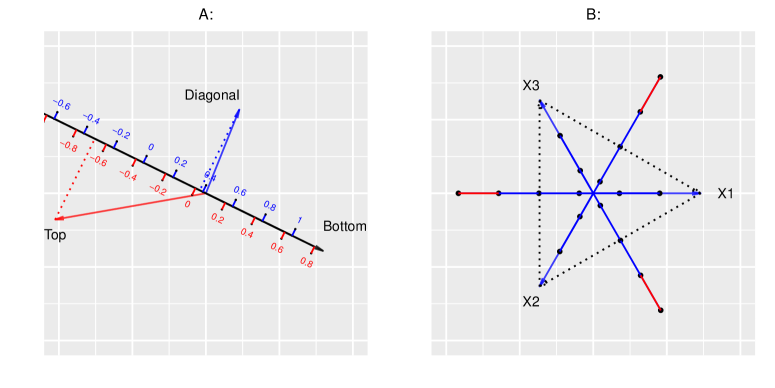
Figure 2: Interpretation of a biplot of the double-centered correlation matrix by the scalar product rule. A: An empirical $3\times 3$ correlation matrix with double calibration of the variable Bottom. The lower scale refers to the projection of Top, the upper scale to the projection of Diagonal. B: An equicorrelation matrix with $r_{ij}=0.20$. Black dots represent increments of 0.2 in the correlation scale.

The remainder of this article presents some theory on possible approximations to the correlation matrix based on weighted alternating least-squares algorithms, and provides software to generate the approximations and visualizations. Visualizations are integrated into the framework of the grammar of graphics (Wilkinson, 2005) making use of the R-package ggplot2 (Wickham, 2016).

2 Materials and methods

We develop methods for the approximation of a correlation matrix by weighted alternating least squares algorithms, and design an algorithm that approximates the correlation matrix while adjusting for column effects. Correlation tally sticks are presented to facilitate the visualization of the approximations. Some generalized root mean squared error (rmse) statistics are proposed that allow the calculation of overall and per-variable goodness-of-fit measures for both symmetric and asymmetric representations that use weights. Several data sets are used to illustrate the approximations.

Optimization problem

The representations of the correlation matrix in the introduction are suboptimal, for they include the diagonal of ones. The fit of the diagonal can be avoided by using a weighted approach using $p\times p$ weight matrix $\mathbf{W}$ with zeros on the diagonal. We seek a symmetric low rank approximation $\mathbf{R}\approx\mathbf{G}\mathbf{G}^{\prime}$ without fitting its diagonal, by minimizing the loss function

$$\sigma(\mathbf{G})=\sum_{i=1}^{p}\sum_{j=1}^{p}w_{ij}(r_{ij}-{\mathbf{g}_{i}}^{\prime}\mathbf{g}_{j})^{2}.$$ (1)

For equal weights ($\mathbf{W}=\mathbf{J}=\mathbf{1}\mathbf{1}^{\prime}$), Eq. (1) is solved by the eigenvalue-eigenvector decomposition of $\mathbf{R}$, which amounts to a pca of the standardized data matrix. The scalar, column and column–plus–row adjustments presented in the Introduction by using averages can be carried out more generally by minimizing the loss function

$$\sigma(\mathbf{G},\delta,\mathbf{p},\mathbf{q})=\sum_{i=1}^{p}\sum_{j=1}^{p}w_{ij}(r_{ij}-\delta-\mathbf{1}\mathbf{q}^{\prime}-\mathbf{p}\mathbf{1}^{\prime}-{\mathbf{g}_{i}}^{\prime}\mathbf{g}_{j})^{2},$$ (2)

where $\delta$ represents a single scalar adjustment, $\mathbf{q}$ a vector of column adjustments and $\mathbf{p}$ a vector of row adjustments. The more general version of loss function (2), with the factorization $\mathbf{R}\approx\mathbf{A}\mathbf{B}^{\prime}$ is given by

$$\sigma(\mathbf{A},\mathbf{B},\delta,\mathbf{p},\mathbf{q})=\sum_{i=1}^{p}\sum_{j=1}^{p}w_{ij}(r_{ij}-\delta-\mathbf{1}\mathbf{q}^{\prime}-\mathbf{p}\mathbf{1}^{\prime}-{\mathbf{a}_{i}}^{\prime}\mathbf{b}_{j})^{2},$$ (3)

and can be efficiently minimized with the R function wAddPCA (De Leeuw & Graffelman, 2022). Program wAddPCA allows for all possible adjustments, as either $\delta$, $\mathbf{q}$ or $\mathbf{p}$ can be set to zero. To avoid the problems with the biplot interpretation when row and column adjustment is performed (see Figure 2A) one can best either minimize these loss functions using either a single scalar adjustment or a column adjustment only. The latter implies each variable has a single adjustment ($\delta+q_{j}$) which is represented by the origin of the biplot. This is akin to an ordinary cases by variables pca biplot where the origin has the interpretation of representing the mean of each variable, though it differs from pca because the diagonal is turned off by assigning it zero weight. In terms of the calibration of a biplot axis, it means that each biplot vector has a unique zero correlation point, which favours the visualization. Moreover, we suggest to require symmetry, such that $\mathbf{A}=\mathbf{B}$, meaning that we minimize Eq. (2) with $\mathbf{p}=\mathbf{0}$ and seek the decomposition

$$\mathbf{R}=\delta\mathbf{1}\mathbf{1}^{\prime}+\mathbf{1}\mathbf{q}^{\prime}+\mathbf{G}\mathbf{G}^{\prime}+\mathbf{E}.$$ (4)

We note that this gives, counterintuitively, an asymmetric approximation to $\mathbf{R}$, but with a symmetric low rank factorization ($\mathbf{G}\mathbf{G}^{\prime}$), such that there is only a single biplot vector per variable. Note that the asymmetric nature of the approximation implies that $\mathbf{E}+\mathbf{1}\mathbf{q}^{\prime}$ will be symmetric. Because there is an adjustment for each column, we expect that the fit can be better than is obtained by a single scalar adjustment only (i.e. $\mathbf{q}=\mathbf{0}$). The loss function, using the $p\times p$ non-negative unit-sum weight matrix $\mathbf{W}$, can be concisely written as

$$\sigma(\mathbf{G},\delta,\mathbf{q})=\mbox{tr}(\mathbf{E}^{\prime}(\mathbf{W}\circ\mathbf{E})),$$ (5)

where $\circ$ represents the Hadamard product, and $\mathbf{E}$ a $p\times p$ matrix of residuals. Setting first order derivatives w.r.t. $\delta$, $\mathbf{q}$ and $\mathbf{C}$ equal to zero, we respectively obtain

$$\delta=\mbox{tr}(\mathbf{W}\circ\mathbf{R})-\mbox{tr}(\mathbf{q}\mathbf{1}^{\prime}\mathbf{W})-\mbox{tr}(\mathbf{W}\mathbf{G}\mathbf{G}^{\prime}),$$ (6)

$$\mathbf{q}=\mathbf{D}_{w}^{-1}\left(\mathbf{W}\circ(\mathbf{R}-\delta\mathbf{J}-\mathbf{G}\mathbf{G}^{\prime})\mathbf{1}\right),$$ (7)

where $\mathbf{D}_{w}=diag(\mathbf{W}\mathbf{1})$, and

$$(\mathbf{W}\circ(\mathbf{R}-\delta\mathbf{J}-\frac{1}{2}(\mathbf{1}\mathbf{q}^{\prime})-\frac{1}{2}(\mathbf{q}\mathbf{1}^{\prime})-\mathbf{G}\mathbf{G}^{\prime}))\mathbf{G}=\mathbf{O}.$$ (8)

Importantly, we note the last equation can be resolved by applying the ipSymLS algorithm (De Leeuw, 2006) to the adjusted form of the correlation matrix

$$\mathbf{R}_{a}=\mathbf{R}-\delta\mathbf{J}-\frac{1}{2}(\mathbf{1}\mathbf{q}^{\prime})-\frac{1}{2}(\mathbf{q}\mathbf{1}^{\prime})-\mathbf{G}\mathbf{G}^{\prime},$$ (9)

for given $\delta$ and $\mathbf{q}$.

Algorithm

An iterative algorithm can now be set up by:

1. Choosing initial values for $\delta$ (e.g.  $\delta=0$) and $\mathbf{q}$ (e.g.  the column means of $\mathbf{R}$).

2. Calculate $\mathbf{G}$, resolving Eq. (8) with ipSymLS for given rank of interest.

3. Update $\delta$ according to Eq. (6).

4. Return to step 2. and iterate until convergence.

5. Update $\mathbf{q}$ according to Eq. (7).

6. Return to step 2. and iterate until convergence.

These steps have been programmed in function FitRDeltaQSym of the R package Correlplot (Graffelman & De Leeuw, 2023a). A biplot of the adjusted correlation matrix is obtained by plotting the rows of $\mathbf{G}$. In the remainder, we will refer to the different options of the wals algorithm as wals-null (no adjustments), wals-$\delta$ (only a scalar adjustment), wals-$q$ (only column adjustment), wals-$q$-sym (only column adjustment but with symmetric factorization (Eq. 4)) and wals-$p$-$q$ (row and column adjustment).

Zero correlation point

For the purpose of interpretation, it is convenient to find the point of zero correlation on each biplot vector, and mark it on each biplot vector. After convergence, we have the approximation

$$\mathbf{R}-\delta\mathbf{J}-\mathbf{1}\mathbf{q}^{\prime}\approx\mathbf{G}\mathbf{G}^{\prime}$$ (10)

which implies

$$r_{ij}-\delta-q_{j}\approx\mathbf{g}_{i}^{\prime}\mathbf{g}_{j}=||\mathbf{g}_{i}||||\mathbf{g}_{j}||\cos{\theta}=||\mathbf{g}_{j}||||\mathbf{p}_{ij}||,$$ (11)

where $\mathbf{p}_{ij}$ is the projection of $\mathbf{g}_{i}$ onto $\mathbf{g}_{j}$. This projection is proportional to $\mathbf{g}_{j}$, and given by

$$\mathbf{p}_{ij}=\frac{\mathbf{g}_{i}^{\prime}\mathbf{g}_{j}}{\mathbf{g}_{j}^{\prime}\mathbf{g}_{j}}\mathbf{g}_{j}\approx\frac{r_{ij}-\delta-q_{j}}{\mathbf{g}_{j}^{\prime}\mathbf{g}_{j}}\mathbf{g}_{j}.$$ (12)

By substituting $r_{ij}=0$ in the latter equation, the coordinates of the zero correlation point on biplot vector $\mathbf{g}_{j}$ are found. Obviously, the coordinates of other values of interest (1, -1, etc.) can be found in the same way. In matrix terms, all zero points can be found simultaneously with the expression

$$-diag(\delta+\mathbf{q})\mathbf{D}_{g}^{-1}\mathbf{G}\quad\mbox{ with }\mathbf{D}_{g}=diag(\mathbf{G}\mathbf{G}^{\prime}).$$ (13)

The latter equations can be used to create an equally spaced correlation tally stick, where the values $(-1.0,-0.8,-0.6,\ldots,+1.0)$ are marked off as small dots on the biplot vector to facilitate reading off the approximation of the correlations without cluttering up the biplot with a fully calibrated scale with all its tick marks and tick mark labels. Colouring the biplot vector according to the sign of the approximated correlation (e.g., red for negative, blue for positive) further enhances the visualization (See Figures 2B, 3 and 4).

Goodness-of-fit

We provide a generic formula for calculating the rmse of an approximation to the correlation matrix from the error matrix $\mathbf{E}$, which takes into account that the approximation may not be symmetric,

$$RMSE=\sqrt{\frac{\sum_{i=1}^{p}\sum_{j=1}^{p}w_{ij}e_{ij}^{2}}{\sum_{i=1}^{p}\sum_{j=1}^{p}w_{ij}}}=\sqrt{\frac{\sum_{i\not=j}^{p}w_{ij}e_{ij}^{2}+\sum_{i}w_{ii}e_{ii}^{2}}{\sum_{i=1}^{p}\sum_{j=1}^{p}w_{ij}}}.$$ (14)

This expression allows for weighting by means of a symmetric non-negative weight matrix. The exclusion of the diagonal from the rmse calculation is possible by setting the diagonal of the weight matrix to zero. Likewise, the per-variable rmse, $z_{i}$, can be calculated with

$$z_{i}=\sqrt{\frac{\sum_{j=1}^{p}w_{ij}e_{ij}^{2}+\sum_{j=1}^{p}w_{ji}e_{ji}^{2}-w_{ii}e_{ii}^{2}}{\sum_{j=1}^{p}w_{ij}+\sum_{j=1}^{p}w_{ji}-w_{ii}}}=\sqrt{\frac{\sum_{j=1}^{p}w_{ij}e_{ij}^{2}+\sum_{j=1}^{p}w_{ji}e_{ji}^{2}-w_{ii}e_{ii}^{2}}{2\sum_{j=1}^{p}w_{ij}-w_{ii}}}.$$ (15)

where the terms $w_{ii}e_{ii}^{2}$ and $w_{ii}$ occur to avoid double-counting the errors on the diagonal. The overall rmse obviously relates to the per-variable rmse, and this relation is found to be

$$RMSE=\sqrt{\frac{\frac{1}{2}\sum_{i}z_{i}^{2}\left(2\sum_{j=1}^{p}w_{ij}-w_{ii}\right)+\frac{1}{2}\sum_{i}w_{ii}(r_{ii}-\hat{r}_{ii})^{2}}{\sum_{i=1}^{p}\sum_{j=1}^{p}w_{ij}}}.$$ (16)

Whenever the diagonal is turned off, this simplifies to

$$RMSE=\sqrt{\frac{\sum_{i}z_{i}^{2}\left(\sum_{j=1}^{p}w_{ij}\right)}{\sum_{i=1}^{p}\sum_{j=1}^{p}w_{ij}}}=\sqrt{\frac{\sum_{i}z_{i}^{2}w_{i.}}{\sum_{i=1}^{p}w_{i.}}},$$ (17)

where $w_{i.}$ is the total marginal weight for the $i$th variable. The latter expression is the square root of a weighted average of the squared rmses of each variable.

3 Results

We give a few examples of the method we have developed. Table 1 shows the rmse statistics for a few correlation matrices, analysed in more detail below, obtained by ten different methods: pca, the svd of $\mathbf{R}_{o}$ (adjustment by subtracting its overall mean), the svd of $\mathbf{R}_{c}$ (adjustment by column-centring), the svd of $\mathbf{R}_{dc}$ (adjustment by double-centring), principal factor analysis (pfa), and wals with different adjustments. All applications of wals used zero weights for the diagonal, and we consecutively used no adjustment (wals-null), scalar adjustment only (wals-$\delta$), column adjustment with symmetric factorization (wals-$q$-sym), column adjustment without symmetry (wals-$q$) and adjustment of both rows and columns (wals-$p$-$q$). pca and the three svds try to approximate the diagonal of the correlation matrix, and the corresponding rmse calculations include the diagonal, whereas for pfa and wals the diagonal was excluded from rmse calculations. Table 1 list the methods in order of expected decrease of the rmse. For wals, non-compliance of that order is typically indicative of non-convergence of one the algorithms.

	Dataset
Method	Goblets	Milks	Beans
pca $\mathbf{R}$	0.0696	0.1183	0.1761
svd $\mathbf{R}_{o}$	0.0749	0.0813	0.1950
svd $\mathbf{R}_{c}$	0.0440	0.0550	0.1202
svd $\mathbf{R}_{dc}$	0.0210	0.0431	0.0997
pfa	0.0417	0.0515	0.1097
wals-nul.	0.0417	0.0514	0.1097
wals-$\delta$	0.0417	0.0497	0.1062
wals-$q$-sym	0.0186	0.0146	0.1034
wals-$q$	0.0197	0.0140	0.0991
wals-$p$-$q$	0.0018	0.0003	0.0693

Table 1: Goodness-of-fit statistics (rmse) for three correlation matrices obtained by using different methods. rmses for the svds (above the dashed line) include the diagonal of the correlation matrix, for pfa and wals variants the diagonal was excluded.

3.1 Archeological goblets data

We analyse the correlation matrix of six size measurements (rim diameter RD; bowl width BW; bowl height BH; foot diameter FD; width at the top of the stem SW; and stem height SH) of a sample of 25 archeological goblets from Thailand (Manly, 1989) and given in Table 2.

	SH	FD	BW	BH	RD	SW
SH	1.000	0.910	0.797	0.858	0.588	0.289
FD	0.910	1.000	0.829	0.843	0.675	0.487
BW	0.797	0.829	1.000	0.839	0.623	0.581
BH	0.858	0.843	0.839	1.000	0.346	0.251
RD	0.588	0.675	0.623	0.346	1.000	0.690
SW	0.289	0.487	0.581	0.251	0.690	1.000

Table 2: Correlation matrix of Manly’s Goblets data.

Figure 3 shows three biplots of the correlation matrix obtained by a standard correlation-based pca (3A), wals-$\delta$ (3B) and wals-$q$-sym (3C). In this case, the last analysis gives the lowest rmse (0.0186). pca knots all biplot vectors at correlation zero in the origin. wals-$\delta$ knots all biplot vectors at correlation $\delta=-0.72$ in the origin. In the last analysis (3C), each biplot vector has it own specific correlation represented by the origin, which gives additional flexibility to fit the correlation matrix and allows for reduction of the rmse (see Table 1). Figure 3C displays a long stretching of the vectors RD and SW, whose end points are outliers that are out of the plot. Consequently there is a high rate of change of the correlation along these two vectors. Standard correlation tally sticks with 0.2 unit changes are shown for RD and SW; an additional correlation stick for BW is shown with black dots for correlations (0.75, 0.80 and 0.85). The rate of change of the correlation for the shorter vector BW, as well as for the other three shorter vectors is much lower. Table 3 shows all variables achieve smaller rmse in the last representation, but that the stretching benefits RD and SW in particular, whose rmse is reduced about eight to ten-fold in comparison with using a scalar adjustment only. The four short vectors for SH, FD and BW with BH emphasize these variables form an approximately equicorrelated block in the correlation matrix, and that their correlations with the stretched pair RD and SW show more variation. Correlations in Table 2 were, a posteriori, conveniently ordered to confirm this detected feature of the correlation matrix.

Dataset	Method	RD	BW	BH	FD	SW	SH
Goblets	pca	0.0901	0.0637	0.0506	0.0384	0.0762	0.0535
	wals-$\delta$	0.0454	0.0427	0.0408	0.0278	0.0401	0.0471
	wals-$q$-sym	0.0044	0.0174	0.0110	0.0268	0.0051	0.0299
		Density	Fat	Protein	Casein	Dry	Yield
Milk	pca	0.1692	0.0677	0.0912	0.0681	0.0831	0.1122
	wals-$\delta$	0.0683	0.0437	0.0238	0.0052	0.0621	0.0563
	wals-$q$-sym	0.0044	0.0147	0.0062	0.0134	0.0197	0.0209
		Area	PM	MjAl	MiAL	AR	EXT	SOL	ROU	SF2	SF4
Beans	pca	0.0660	0.0798	0.0317	0.1596	0.2173	0.2118	0.1939	0.0865	0.1323	0.2110
	wals-$\delta$	0.0605	0.0653	0.0664	0.1444	0.1767	0.0444	0.1389	0.0523	0.1095	0.1116
	wals-$q$-sym	0.0503	0.0646	0.0636	0.1286	0.1528	0.0384	0.1523	0.0731	0.1159	0.1133

Table 3: Per-variable goodness-of-fit statistic (rmse) for the datasets Goblets, Milk and Beans, using three methods.

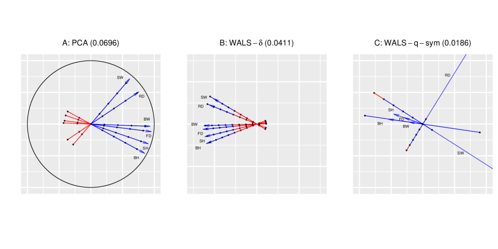
Figure 3: Biplots of archeological goblets. A: pca biplot of the correlation matrix. B: wals-$\delta$ biplot ($\delta=-0.72$). C: wals-$q$-sym biplot. Black dots represent increments of 0.2 in the correlation scale. Blue tails correspond to the positive part of the correlation scale, red tails to the negative part. The rmse of the approximation is given in the title of each panel.

3.2 Milk data

We analyse the correlation matrix of six variables registred on 85 milks (Density, Fat, Protein, Casein, Dry and Yield), available in the FactoMineR package (Lê et al., 2008) and based on a study by Daudin et al. (1988). The correlation matrix of the variables is shown in Table 4.

	Density	Fat	Protein	Casein	Dry	Yield
Density	1.000	0.402	0.543	0.596	0.753	0.432
Fat	0.402	1.000	0.446	0.430	0.683	0.652
Protein	0.543	0.446	1.000	0.958	0.668	0.641
Casein	0.596	0.430	0.958	1.000	0.695	0.617
Dry	0.753	0.683	0.668	0.695	1.000	0.700
Yield	0.432	0.652	0.641	0.617	0.700	1.000

Table 4: Correlation matrix of Daudin’s milk data, as included in the FactoMineR package.

Figure 4 shows the three biplots obtained by pca, wals-$\delta$ and wals-$q$-sym. The tight relationship between Protein and Casein is visible in all plots. The $\delta$ adjustment gives a considerable reduction in rmse with respect to pca, and the column-adjustment with symmetric decomposition further reduces the rmse. Indeed, the latter two-dimensional representation of the correlation matrix is close to perfect. In this case, when using the $\delta$ adjustment (Figure 4B), a large negative value of the adjustment parameter is obtained ($\delta=-2.16$) which is out of the range of the correlation scale. This emphasizes that for this data, with considerable positive correlations for all variables, the origin of the biplot is ultimately uninteresting; it is the zero in the correlation scale on the biplot vector that is actually needed for adequate visualization and interpretation of the correlation structure. When a column-adjustment with symmetric factorization is used, variable Density becomes an outlier (off the plot) and its biplot vector is largely stretched and consequently the projections onto this vector change fast as shown by the standard tally stick on Density. To the contrary, variables Dry and Yield have very short biplot vectors such that their correlations hardly change across the biplot. To illustrate this, Figure 4C shows the customized tally stick of Yield that spans the range (0.63, 0.68) with 0.01 increments. This emphasizes, outlier Density taken apart, the approximate equicorrelation of Dry and Yield with all other variables. The per-variable rmse in Table 3 shows the variable that is most stretched, Density, experiments the largest reduction in rmse when the column-adjustment is used.

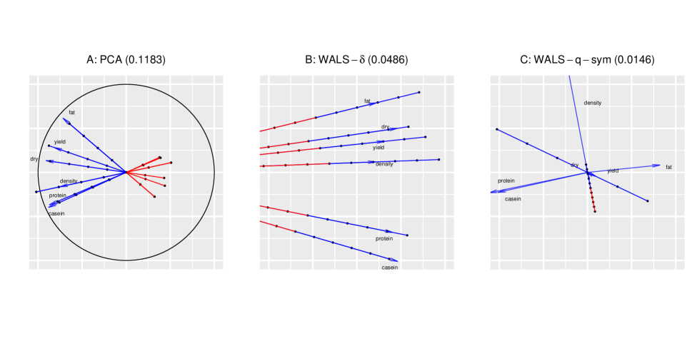
Figure 4: Biplots of milk data correlation structure. A: pca biplot of the correlation matrix. B: wals-$\delta$ biplot ($\delta=-2.16$). C: wals-$q$-sym biplot. Black dots represent increments of 0.2 in the correlation scale. Blue tails correspond to the positive part of the correlation scale, red tails to the negative part. The rmse of the approximation is given in the title of each panel.

3.3 Dry bean data

We present an analysis of a larger correlation matrix of 16 measurements taken on 3546 dry beans of the variety Dermason (Koklu & Özkan, 2020) available at the UCI Machine Learning Repository (https://archive.ics.uci.edu/datasets). The 16 variables are Area, Perimeter (PM), MajorAxisLength (MjAL), MinorAxisLength (MiAL), AspectRatio (AR), Eccentricity (ECC), ConvexArea (CA), EquivDiameter (ED), Extent (EXT), Solidity (SOL), Roundness (ROU), Compactness (COM) and four Shape factors (SF1, SF2, SF3 and SF4). These variables capture different aspects of the size and the shape of the beans, and their correlation matrix is shown in Table 5.

	Area	PM	MjAL	MiAL	AR	ECC	CA	ED	EXT	SOL	ROU	COM	SF1	SF2	SF3	SF4
Area	1.00	0.97	0.92	0.91	0.13	0.15	1.00	1.00	-0.01	0.23	-0.04	-0.14	-0.90	-0.67	-0.14	0.04
PM	0.97	1.00	0.95	0.83	0.25	0.26	0.97	0.97	-0.06	0.05	-0.27	-0.26	-0.83	-0.74	-0.26	-0.05
MjAL	0.92	0.95	1.00	0.68	0.50	0.51	0.92	0.92	-0.08	0.16	-0.25	-0.50	-0.68	-0.90	-0.50	-0.00
MiAL	0.91	0.83	0.68	1.00	-0.29	-0.27	0.91	0.91	0.07	0.25	0.19	0.28	-1.00	-0.31	0.28	0.06
AR	0.13	0.25	0.50	-0.29	1.00	0.98	0.13	0.13	-0.19	-0.08	-0.57	-1.00	0.29	-0.81	-0.99	-0.08
ECC	0.15	0.26	0.51	-0.27	0.98	1.00	0.15	0.15	-0.18	-0.06	-0.54	-0.99	0.27	-0.83	-0.99	-0.06
CA	1.00	0.97	0.92	0.91	0.13	0.15	1.00	1.00	-0.02	0.21	-0.05	-0.14	-0.90	-0.67	-0.14	0.03
ED	1.00	0.97	0.92	0.91	0.13	0.15	1.00	1.00	-0.01	0.23	-0.04	-0.14	-0.91	-0.67	-0.14	0.04
EXT	-0.01	-0.06	-0.08	0.07	-0.19	-0.18	-0.02	-0.01	1.00	0.14	0.21	0.19	-0.07	0.14	0.19	0.09
SOL	0.23	0.05	0.16	0.25	-0.08	-0.06	0.21	0.23	0.14	1.00	0.73	0.09	-0.26	-0.07	0.09	0.51
ROU	-0.04	-0.27	-0.25	0.19	-0.57	-0.54	-0.05	-0.04	0.21	0.73	1.00	0.57	-0.21	0.44	0.57	0.38
COM	-0.14	-0.26	-0.50	0.28	-1.00	-0.99	-0.14	-0.14	0.19	0.09	0.57	1.00	-0.29	0.82	1.00	0.11
SF1	-0.90	-0.83	-0.68	-1.00	0.29	0.27	-0.90	-0.91	-0.07	-0.26	-0.21	-0.29	1.00	0.31	-0.28	-0.09
SF2	-0.67	-0.74	-0.90	-0.31	-0.81	-0.83	-0.67	-0.67	0.14	-0.07	0.44	0.82	0.31	1.00	0.82	0.05
SF3	-0.14	-0.26	-0.50	0.28	-0.99	-0.99	-0.14	-0.14	0.19	0.09	0.57	1.00	-0.28	0.82	1.00	0.10
SF4	0.04	-0.05	-0.00	0.06	-0.08	-0.06	0.03	0.04	0.09	0.51	0.38	0.11	-0.09	0.05	0.10	1.00

Table 5: Correlation matrix of the Dry bean data for variety Dermason.

Biplots of the correlation structure are shown in Figure 5. Figure 5A shows a standard pca correlation biplot, which has a rmse of 0.1336. This reveals several variables are almost perfectly correlated, suggesting redundancy in some of the defined variables, where (SF3, COM, ECC, AR) apparently measure the same thing, as well as (SF1, MiAl), and (Area, ED, CA). We repeated pca retaining only one variable of each of these three groups, so reducing the number of variables to ten. Figure 5B shows the biplot with the reduced dataset, where the rmse has increased to 0.1761 due to the elimination of large part of the redundancy in the data. Figure 5C shows the biplot obtained by using the wals-$\delta$; this considerably improves the goodness-of-fit of the correlation matrix (rmse 0.1062); the origin of this plots represents $\delta=-0.12$. In general, correlations fitted by wals-$\delta$ are lower (i.e.  closer to zero) than those obtained by pca.

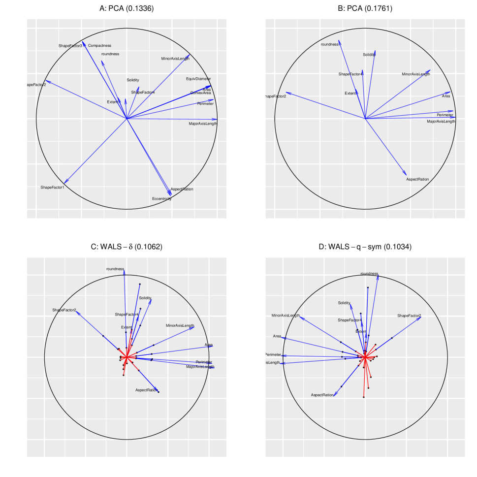
Figure 5: Biplots of the Beans data correlation structure. A: pca biplot of the original correlation matrix. B: pca biplot of the reduced correlation matrix. C: wals-$\delta$ biplot ($\delta=-0.12$). C: wals-$q$-sym biplot. Black dots represent increments of 0.2 in the correlation scale; only the (-0.2,0,0.2) part of the scale is indicated. Blue tails correspond to the positive part of the correlation scale, red tails to the negative part. The rmse of the approximation is given in the title of each panel.

The wals-$q$-sym biplot only slightly decreases the rmse (0.1034) in comparison with the wals-$\delta$ biplot. In this case, the column adjustment does not lead to a significant improvement of the approximation (See Table 2). The wals-$q$-sym biplot appears similar to the wals-$\delta$ when the latter is reflected in the vertical axis. However, the latter no longer has a common correlation for the origin, and some of the variables have slightly worsened their representation while others have slightly improved (see detailed rmse statistics in Table  3).

4 Discussion

In this article we have considered approximations and visualizations of a fundamental matrix in multivariate analysis, the correlation matrix. From a purely numerical point of view, the best approximation, in the weighted least squares sense, is obtained by performing weighted alternating least squares with row and column adjustment (as illustrated by the examples in Table 1). This is natural, because the use of both row and column adjustment offers most flexibility to fit the correlations. The optimal approximation is however, particularly hard to visualize by using scalar products as has been illustrated in Figure 2A. We have previously reported (Graffelman & De Leeuw, 2023b) on the equivalence of the approximation of $\mathbf{R}$ by wals and the analysis of the double-centered correlation matrix proposed by Hills (1969), when unit weights are used. We note that, with the use of zero weights for the diagonal, the row and column adjustments obtained by wals are no longer equivalent to a double-centering the correlation matrix; in this case wals will give a lower rmse than is obtained by Hills’ double-centered analysis.

By using only a column adjustment but requiring a symmetric low-rank factorization, visualization of the correlations by means of scalar products in a biplot becomes feasible, as shown in the examples in Figures 3C, 4C and 5D. The examples show this representation tends identify equicorrelation structure, where variables that equicorrelate with others collapse to the origin. An inconvenience of this representation is that the approximation is asymmetric in the sense that the projection of $x_{1}$ onto $x_{2}$ gives a numerically different approximation to $r_{12}$ than the reverse projection. For the empirical examples we have studied so far, these differences tended to be small. The representation of the correlation matrix by a single scalar adjustment, as previously advocated (Graffelman & De Leeuw, 2023b), does not suffer from this assymetry but will have a larger rmse. Admittedly, the decrease in rmse obtained by using a column adjustment with symmetric factorization was found to be small in most cases hitherto studied, and the $\delta$-only representation may therefore be favoured for retaining the symmetry of approximation. wals-$q$-sym has been developed here for the fundamental sake of optimality, in order to identify the best approximation to the correlation matrix that can still be visualized.

The column centring of the correlation matrix is inconvenient, because it complicates the visualization by doubling the number of biplot vectors as shown in Figure 1C. One may try to match the two sets of biplot vectors by Procrustes rotation (Gower, 1971) or by the more flexible distance-based matching approach (De Leeuw, 2011). In the case of a perfect match it may be argued one set of biplot vectors could be omitted. In practice, such perfect matches were not observed.

Column and/or row adjustments are common operations for many multivariate methods, where the data matrix is often centered (e.g., in pca) or sometimes double centred prior to the use of the spectral decomposition or the singular value decomposition. In these cases the optimal values for the adjustment parameters for columns or rows are known prior to analysis, in particular if no weighting is applied. For the analysis with a single scalar adjustment $\delta$, there is no closed form solution available for finding $\delta$. Estimating $\delta$ with the overall mean of the correlation matrix seems intuitive, but is suboptimal, and can even worsen the representation in comparison with standard pca, as the examples in Table 1 clearly show. One needs to run the wals algorithm to obtain the optimal value for $\delta$.

The use of correlation tally sticks in biplots of correlation structure is advocated, not only for biplots obtained by wals but also for the standard correlation biplots obtained by pca. They increase the information content of the plot without overcrowding it. Moreover, the rate of change of a correlation along a biplot vector can differ considerably across biplot vectors, and the tally stick makes this clearly visible.

5 Acknowledgements

This work was supported by the Spanish Ministry of Science and Innovation and the European Regional Development Fund under grant PID2021-125380OB-I00 (MCIN/AEI/FEDER); and the National Institutes of Health under Grant GM075091.

The author reports there are no competing interests to declare.

SUPPLEMENTARY MATERIAL

R-package Correlplot:

R-package Correlplot (version 1.1.0) has been updated, and contains code to calculate the approximations to the correlation matrix and to create the graphics shown in the article, for both R’s base graphics environment as well as for the ggplot graphics. R-package Correlplot has a vignette containing a detailed example showing how to generate all graphical representations of the correlation matrix (GNU zipped tar file).

References

- (1)
- Daudin et al. (1988) Daudin, J., Duby, C. & Trecourt, P. (1988), ‘Stability of principal component analysis studied by the bootstrap method’, Statistics 19(2), 241–258.
- De Leeuw (2006) De Leeuw, J. (2006), ‘A decomposition method for weighted least squares low-rank approximation of symmetric matrices’, Department of Statistics, UCLA . Retrieved from https://escholarship.org/uc/item/1wh197mh.
- De Leeuw (2011) De Leeuw, J. (2011), ‘Distance-based transformations of biplots’, Department of Statistics, UCLA . Retrieved from https://escholarship.org/uc/item/0bd8s7fk.
- De Leeuw & Graffelman (2022) De Leeuw, J. & Graffelman, J. (2022), ‘wAddPCA’, Department of Statistics, UCLA . Retrieved from https://jansweb.netlify.app/publication/deleeuw-graffelman-e-22-e/.
- Eckart & Young (1936) Eckart, C. & Young, G. (1936), ‘The approximation of one matrix by another of lower rank’, Psychometrika 1(3), 211–218.
- Gower (1971) Gower, J. C. (1971), Statistical methods of comparing different multivariate analysies of the same data, in F. R. Hodson, D. G. Kendall & P. Tautu, eds, ‘Mathematics in the archaeological and historical sciences’, Edinburgh university press, Edinburgh, pp. 138–149.
- Gower et al. (2011) Gower, J. C., Gardner Lubbe, E. & Le Roux, N. (2011), Understanding biplots, John Wiley, Chichester.
- Gower & Hand (1996) Gower, J. C. & Hand, D. J. (1996), Biplots, Chapman & Hall, London.
- Graffelman & De Leeuw (2023a) Graffelman, J. & De Leeuw, J. (2023a), Correlplot: A Collection of Functions for Graphing Correlation Matrices. https://www.r-project.org, http://www-eio.upc.es/ jan/.
- Graffelman & De Leeuw (2023b) Graffelman, J. & De Leeuw, J. (2023b), ‘Improved approximation and visualization of the correlation matrix’, The American Statistician 77(4), 432–442.
- Graffelman & van Eeuwijk (2005) Graffelman, J. & van Eeuwijk, F. A. (2005), ‘Calibration of multivariate scatter plots for exploratory analysis of relations within and between sets of variables in genomic research’, Biometrical Journal 47(6), 863–879.
- Hills (1969) Hills, M. (1969), ‘On looking at large correlation matrices’, Biometrika 56(2), 249–253.
-
Koklu & Özkan (2020)
Koklu, M. & Özkan, I. A. (2020), ‘Multiclass classification of dry beans using computer vision and machine
learning techniques’, Comput. Electron. Agric. 174, 105507.
https://api.semanticscholar.org/CorpusID:219762890 - Lê et al. (2008) Lê, S., Josse, J. & Husson, F. (2008), ‘FactoMineR: A package for multivariate analysis’, Journal of Statistical Software 25(1), 1–18.
- Manly (1989) Manly, B. F. J. (1989), Multivariate statistical methods: a primer, Chapman and Hall, London.
- Weisberg (2005) Weisberg, S. (2005), Applied Linear Regression, third edn, John Wiley & Sons, New Jersey.
-
Wickham (2016)
Wickham, H. (2016), ggplot2: Elegant
Graphics for Data Analysis, Springer-Verlag New York.
https://ggplot2.tidyverse.org - Wilkinson (2005) Wilkinson, L. (2005), The grammar of graphics, 2nd edn, Springer-Verlag New York.