On positively divisible non-Markovian processes

Abstract

Abstract There are some positively divisible non-Markovian processes whose transition matrices satisfy the Chapman-Kolmogorov equation. These processes should also satisfy the Kolmogorov consistency conditions, an essential requirement for a process to be classified as a stochastic process. Combining the Kolmogorov consistency conditions with the Chapman-Kolmogorov equation, we derive a necessary condition for positively divisible stochastic processes on a finite sample space. This necessary condition enables a systematic approach to the manipulation of certain Markov processes in order to obtain a positively divisible non-Markovian process. We illustrate this idea by an example and, in addition, analyze a classic example given by Feller in the light of our approach.

My inclination has always been to look for general theories and to avoid computation. A discussion I once had with Feller in a New York subway illustrates this attitude and its limitations. We were discussing the Markov property and I remarked that the Chapman-Kolmogorov equation did not make a process Markovian. This statement satisfied me, but not Feller, who liked computation and examples as well as theory. It was characteristic of our attitudes that at first he did not believe me but then went to the trouble of constructing a simple example to prove my assertion. - J. L. Doob [1]

I Introduction

Markov processes are defined by two essential ingredients: $(i)$ the Chapman-Kolmogorov equation and $(ii)$ an initial probability distribution.[2] It may seem that these two features would determine uniquely whether a process is Markovian or not. However, as first noted by Doob to Feller, these two features yield are necessary but not sufficient condition for the Markovianity of a given stochastic process. This observation was also made by Lévy, who analyzed processes that satisfy the aforementioned conditions but are still not Markovian.[3] The first concrete example was proposed by Feller.[4] According to Feller, these kinds of processes are rather ”pathological” and, therefore, the conditions $(i)$ and $(ii)$ can be considered as the characteristic properties that determine Markov processes uniquely.[5] However, other examples were given later for both a countable state space [2] and a continuous state space. [6]

A clear-cut understanding of the distinction between Markovian and non-Markovian processes is important in the theory of classical stochastic processes. [7, 8, 9] In this context, the problem of distinguishing Markovian and non-Markovian processes is particularly relevant for non-Markovian processes which are positively divisible (see Definition 1 below).[10, 11, 12] In the present paper, in contrast to McCauley’s approach to the investigation of positively divisible non-Markovian processes which are based on stochastic differential equations [6], we propose a necessary condition in terms of transition matrices for the existence of non-Markovian processes in the classical regime within finite state space which have the property of being positively divisible. We obtain this condition by combining the Kolmogorov consistency conditions with the Chapman-Kolmogorov equation. We also argue that positively divisible non-Markovian processes are not pathological as they can be obtained by modifying specific Markov processes, using the necessary condition.

The paper is organized as follows. We first recall some definitions of both stochastic processes and Markov processes within finite state space and introduce some conventions in Section II. In Section III we derive a necessary condition for a positively divisible non-Markovian process. In Section IV, we analyze a well-known example designed by Feller [4], and construct a positively divisible non-Markovian process by manipulating a certain Markov process, using our necessary condition. We also apply this example to a certain epidemic situation. We finally draw some conclusions in Section V.

II Markov processes and their characteristic properties

We assume a probability space $\{\Omega,\mathcal{A},\mu\}$ with finite sample space $\Omega=\{\omega_{1},\omega_{2},\ldots,\omega_{n}\}$, $\sigma$-algebra $\mathcal{A}$ on $\Omega$, and probability measure $\mu:\mathcal{A}\rightarrow\mathbb{R}$. We further consider a stochastic process $X:\Omega\times T\rightarrow\mathbb{E}\subseteq\mathbb{R}$ for a set of discrete time steps $T=\{t_{0},t_{1},\ldots\}$. For our purpose, we assume that $\mathbb{E}=\{0,1,\ldots,d-1\}$ for some positive natural number $d\in\mathbb{N}$ unless otherwise stated. Then, the probability measure of $X_{t_{k}}$ is defined as $P\{X_{t_{k}}=j_{k}\}:=\mu(B_{j_{k}})$ such that $B_{j_{k}}=\{\omega\in\Omega\mid X_{t_{k}}(\omega)=j_{k},j_{k}\in\mathbb{E}\}$. In the following, we denote the process as $X(T)=\{X_{t}\mid t\in T\}$. From a physical perspective, one of the main problems about a stochastic process is to investigate the probabilistic characterization of how the random variables $X_{t}$ at different times are related to each other. The study of this problem is mainly based on introducing the joint probability distributions of finite order $m$ defined by means of

$$P_{m}\{X_{t_{m}}=j_{m},X_{t_{m-1}}=j_{m-1},\ldots,X_{t_{1}}=j_{1}\}:=\mu(B_{j_{m}},B_{j_{m-1}},\ldots,B_{j_{1}}),$$ (1)

where we have any ordered set of time instants $t_{1},t_{2},\ldots,t_{m}\in T$, satisfying $t_{1}\leq t_{2}\leq\ldots\leq t_{m}$, and their corresponding random variables $X_{t_{1}},X_{t_{2}},\ldots,X_{t_{m}}\in X(T)$. This joint probability of order $m$ represents the probability that the time-dependent random variable $X_{t}$ takes some value $j_{1}$ at time instant $t_{1}$, some value $j_{2}$ at time instant $t_{2}$, etc. For each value $m=1,2,\ldots$ and each sequence of time instants $t_{1},t_{2},\ldots,t_{m}$, there corresponds a joint probability distribution of order $m$, and all together are called the family of the finite joint probability distribution of the stochastic process $X(T)$, which has to satisfy the following Kolmogorov consistency conditions,

1. $P_{m}\{X_{t_{m}}\in\mathbb{E},X_{t_{m-1}}\in\mathbb{E},\ldots,X_{t_{1}}\in\mathbb{E}\}=1$,

2. $P_{m}\{X_{t_{m}}=j_{m},X_{t_{m-1}}=j_{m-1},\ldots,X_{t_{1}}=j_{1}\}\geq 0$,

3. $P_{m}\{X_{t_{\pi(m)}}=j_{\pi(m)},\ldots,X_{t_{\pi(1)}}=j_{\pi(1)}\}=P_{m}\{X_{t_{m}}=j_{m},\ldots,X_{t_{1}}=j_{1}\}$,

4. For all $1\leq k\leq m$ we have:

   $$P_{m-1}\{X_{t_{m}}=j_{m},\ldots,X_{t_{k+1}}=j_{k+1},X_{t_{k-1}}=j_{k-1},\ldots,X_{t_{1}}=j_{1}\}$$

   $$=\sum_{j_{k}\in\mathbb{E}}P_{m}\{X_{t_{m}}=j_{m},\ldots,X_{t_{k+1}}=j_{k+1},X_{t_{k}}=j_{k},X_{t_{k-1}}=j_{k-1},\ldots,X_{t_{1}}=j_{1}\}.$$ (2)

The first two conditions are just a restatement of the conditions in the definition of a probability measure for a joint probability distribution of order $m$, while the third condition states that the probability distributions must be invariant under all permutations $\pi$ of its arguments. The fourth, and most relevant one in the context of this paper, means that any joint probability distribution of order $m-1$ can be obtained from the distribution of order $m$ by summation over all possible values of the random variable $X_{t_{k}}$ at time $t_{k}$. This implies that the family of joint probability distributions of all orders must be consistent with each other in the sense that the marginal probability distributions of lower orders must be the same as those derived by means of the condition in (2). In the following, we specifically refer to the condition in (2) whenever we mention the term consistency condition.

Recalling the conditional probabilities,

$$\begin{split}&P_{l\mid k}\{X_{t_{k+l}}=j_{k+l},\ldots,X_{t_{k+1}}=j_{k+1}\mid X_{t_{k}}=j_{k},\ldots,X_{t_{1}}=j_{1}\}\\ &\quad\quad\quad=\frac{P_{l+k}\{X_{t_{k+l}}=j_{k+l},\ldots,X_{t_{k+1}}=j_{k+1},X_{t_{k}}=j_{k},\ldots,X_{t_{1}}=j_{1}\}}{P_{k}\{X_{t_{k}}=j_{k},\ldots,X_{t_{1}}=j_{1}\}},\end{split}$$ (3)

one can express the joint probability distribution of order $m$ as

$$\begin{split}&P_{m}\{X_{t_{m}}=j_{m},X_{t_{m-1}}=j_{m-1},\ldots,X_{t_{1}}=j_{1}\}\\ &=P_{m-k\mid k}\{X_{t_{m}}=j_{m},\ldots,X_{t_{k+1}}=j_{k+1}\mid X_{t_{k}}=j_{k},\ldots,X_{t_{1}}=j_{1}\}\\ &\quad\times P_{k}\{X_{t_{k}}=j_{k},\ldots,X_{t_{1}}=j_{1}\}.\end{split}$$ (4)

A stochastic process $X_{t}$ is said to be a Markov process if it rapidly forgets its past history such that its future state depends only on its present state. This Markovian feature can be formulated in terms of conditional probabilities as

$$P_{1\mid k}\{X_{t_{k+1}}=j_{k+1}\mid X_{t_{k}}=j_{k},\ldots,X_{t_{1}}=j_{1}\}=P_{1\mid 1}\{X_{t_{k+1}}=j_{k+1}\mid X_{t_{k}}=j_{k}\},$$ (5)

which is known as Markov condition. It is assumed to hold for all $k=1,2,...$ and for all ordered time instants $t_{1}\leq t_{2}\leq\ldots\leq t_{k}\leq t_{k+1}$. The Markov condition implies that the conditional probability $P_{1\mid 1}\{X_{t_{k}}=j_{k}\mid X_{t_{l}}=j_{l}\}$ for $t_{l}\leq t_{k}$ plays a central role in the theory of Markov processes.

Before proceeding further, let us introduce some common abbreviations to simplify notation. To this end, we define $\mathbb{R}_{+}:=\{r\in\mathbb{R}\mid r\geq 0\}$, and introduce the set of probability vectors of dimension $d$ as $\mathbb{P}^{d}=\{(p_{1},p_{2},\ldots,p_{d})^{T}\mid p_{k}\in\mathbb{R}_{+},\sum_{i=1}^{d}p_{i}=1\}$. Then, we define:

1. $p_{m}(j_{k},t_{k};\ldots;j_{1},t_{1}):=P_{m}\{X_{t_{k}}=j_{k},\ldots,X_{t_{1}}=j_{1}\}$ for all $t_{1}\leq\ldots\leq t_{k}\in T$ and $j_{1},\ldots,j_{k}\in\mathbb{E}$,

2. $p_{l\mid k}(j_{k+l},t_{k+l};\ldots;j_{k+1},t_{k+1}\mid j_{k},t_{k};\ldots;j_{1},t_{1}):=P_{l\mid k}\{X_{t_{k+l}}=j_{k+l},\ldots,X_{t_{k+1}}=j_{k+1}\mid X_{t_{k}}=j_{k},\ldots,X_{t_{1}}=j_{1}\}$,

3. $p(j,t\mid j^{\prime},t^{\prime}):=P_{1\mid 1}\{X_{t}=j\mid X_{t^{\prime}}=j^{\prime}\}$ so that $p(j,t\mid j^{\prime},t^{\prime})=p_{1\mid 1}(j,t\mid j^{\prime},t^{\prime})$ for all $t,t^{\prime}\in T$ and for all $j,j^{\prime}\in\mathbb{E}$,

4. $p(j,t):=P_{1}\{X_{t}=j\}$ so that $p(j,t)=p_{1}(j,t)$,

5. $\mathbf{p}(t):=(p(j=0,t),p(j=1,t),\ldots,p(j=d-1,t))^{T}\in\mathbb{P}^{d}$,

where $\mathbf{p}(t)$ is known as one-point probability vector. The conditional probabilities $p(j,t\mid j^{\prime},t^{\prime})$ are also known as transition probabilities. Defining a transition matrix, $T(t,t^{\prime})=(T_{jj^{\prime}}(t,t^{\prime}))$ with $T_{jj^{\prime}}(t,t^{\prime}):=p(j,t\mid j^{\prime},t^{\prime})$, one can write the evolution of the time-dependent random variable $X(T)$ in terms of the transition probabilities as

$$p(j,t) =\displaystyle\sum_{j^{\prime}\in\mathbb{E}}p_{2}(j,t;j^{\prime},t^{\prime})$$

$$=\displaystyle\sum_{j^{\prime}\in\mathbb{E}}p(j,t\mid j^{\prime},t^{\prime})p(j^{\prime},t^{\prime})$$

$$=\displaystyle\sum_{j^{\prime}\in\mathbb{E}}T_{jj^{\prime}}(t,t^{\prime})p(j^{\prime},t^{\prime}),$$ (6)

which takes on the matrix multiplication form,

$$\mathbf{p}(t)=T(t,t^{\prime})\mathbf{p}(t^{\prime}).$$ (7)

In passing, we note that a general transition matrix $T(t,t^{\prime})$, by virtue of its definition, is characterized by the following properties:

1. Its elements are non-negative, $T_{jj^{\prime}}(t,t^{\prime})\geq 0$,

2. $\sum_{j}T_{jj^{\prime}}(t,t^{\prime})=1$ for all $j^{\prime}$,

3. $T_{jj^{\prime}}(t^{\prime},t^{\prime})=\delta_{j,j^{\prime}}$,

4. $p_{2}(j,t;j^{\prime},t^{\prime})=T(j,t\mid j^{\prime},t^{\prime})p(j^{\prime},t^{\prime})$ for all $t\geq t^{\prime}$.

Note that the fourth property implies equation (7).

Let us now assume a joint probability distribution of order $3$, $p_{3}(j_{3},t_{3};j_{2},t_{2};j_{1},t_{1})$ for any $t_{1}\leq t_{2}\leq t_{3}$ which corresponds to a Markov process $X(T)$. Using the Markov condition, one can write

$$\begin{split}p_{3}(j_{3},t_{3};j_{2},t_{2};j_{1},t_{1})&=p_{1\mid 2}(j_{3},t_{3}\mid j_{2},t_{2};j_{1},t_{1})p_{2}(j_{2},t_{2};j_{1},t_{1})\\ &=p(j_{3},t_{3}\mid j_{2},t_{2})p(j_{2},t_{2}\mid j_{1},t_{1})p(j_{1},t_{1}),\end{split}$$ (8)

and summing over $j_{2}$ one gets

$$p_{2}(j_{3},t_{3};j_{1},t_{1})=p(j_{1},t_{1})\displaystyle\sum_{j_{2}\in\mathbb{E}}p(j_{3},t_{3}\mid j_{2},t_{2})p(j_{2},t_{2}\mid j_{1},t_{1}).$$ (9)

Dividing both sides by $p(j_{1},t_{1})$, one obtains the celebrated Chapman-Kolmogorov equation

$$p(j_{3},t_{3}\mid j_{1},t_{1})=\displaystyle\sum_{j_{2}\in\mathbb{E}}p(j_{3},t_{3}\mid j_{2},t_{2})p(j_{2},t_{2}\mid j_{1},t_{1}).$$ (10)

Equation (10) can be put into the form of the multiplication of transition matrices as

$$T(t_{3},t_{1})=T(t_{3},t_{2})T(t_{2},t_{1}).$$ (11)

We note that a complete probabilistic characterization of a Markov process is given by means of the evolution equation (6) and the Chapman-Kolmogorov equation (11).

A classical stochastic process on a finite sample space can also be formalized in a more compact form. To this end, denoting by $\mathbf{p}(0)$ the initial probability vector, the time evolution of the one-point distribution of the process can be described by a time-dependent stochastic matrix $\Lambda(t,0)$ as

$$\mathbf{p}(t)=\Lambda(t,0)\mathbf{p}(0).$$ (12)

A general stochastic matrix $\Lambda(t,0)$ is characterized by two properties:

1. Its elements are non-negative, $\Lambda_{jj^{\prime}}(t,0)\geq 0$,

2. $\sum_{j}\Lambda_{jj^{\prime}}(t,0)=1$ for all $j^{\prime}$.

Accordingly, a stochastic matrix $\Lambda(t,0)$ can be considered as the generalization of a transition matrix by relaxing its third and fourth properties. We say that a stochastic matrix $\Lambda(t,0)$ is divisible if, for any $t\geq s\geq 0$, one can write

$$\Lambda(t,0)=\Lambda(t,s)\Lambda(s,0).$$ (13)

If the stochastic matrix $\Lambda(s,0)$ is invertible, $\Lambda(t,s)$ can be uniquely written as $\Lambda(t,s)=\Lambda(t,0)\Lambda^{-1}(s,0)$. We note that $\Lambda(t,s)$ does not have to be a stochastic matrix. We can now formulate the definition of a P-divisible process:

Definition 1

A stochastic process $X(T)$ which is characterized by the divisible stochastic matrix $\Lambda(t,0)$ is called positively divisible (classical P-divisible) if $\Lambda(t,0)=\Lambda(t,s)\Lambda(s,0)$ such that $\Lambda(t,s)$ is also a stochastic matrix for all $t\geq s\geq 0$.

We stress that if $\Lambda(s,0)$ is not invertible, the stochastic matrix $\Lambda(t,s)$ that satisfies the P-divisibility condition of this definition is not unique in general. Moreover, we see that P-divisibility reduces to the Chapman-Kolmogorov equation if the stochastic matrix under consideration corresponds to the transition matrix of the process. Therefore, we use the following convention: Whenever we speak of the transition matrix of a P-divisible process we refer to a P-divisible stochastic process whose stochastic matrix $\Lambda(t,t^{\prime})$ corresponds to its transition matrix $T(t,t^{\prime})$ for any $t\geq t^{\prime}\geq 0$.

It is evident that Markov processes are P-divisible. As was noted at the beginning, there are some non-Markovian processes satisfying the Chapman-Kolmogorov equation which are P-divisible according to Definition 1.[4, 6] Moreover, it was shown by construction that there are also P-divisible processes which belong to the class of semi-Markovian processes and are non-Markovian.[10] In the next section, we derive a necessary condition in terms of transition matrices for P-divisible non-Markovian processes.

III A necessary condition for P-divisible non-Markovian processes

We consider a stochastic process $X(T)$ as defined in section II, and its joint probability distribution of order $3$, $p_{3}(j_{3},t_{3};j_{2},t_{2};j_{1},t_{1})$, for the time steps $t_{1}\leq t_{2}\leq t_{3}$. Using the consistency condition and equation (4), we can write

$$\begin{split}p(j_{3},t_{3};j_{1},t_{1})&=\displaystyle\sum_{j_{2}\in\mathbb{E}}p_{3}(j_{3},t_{3};j_{2},t_{2};j_{1},t_{1})\\ &=\displaystyle\sum_{j_{2}\in\mathbb{E}}p_{1\mid 2}(j_{3},t_{3}\mid j_{2},t_{2};j_{1},t_{1})p_{2}(j_{2},t_{2};j_{1},t_{1})\\ &=\displaystyle\sum_{j_{2}\in\mathbb{E}}p_{1\mid 2}(j_{3},t_{3}\mid j_{2},t_{2};j_{1},t_{1})p(j_{2},t_{2}\mid j_{1},t_{1})p(j_{1},t_{1}),\end{split}$$ (14)

and dividing both sides by $p(j_{1},t_{1})$ we derive the conditional probability

$$p(j_{3},t_{3}\mid j_{1},t_{1})=\displaystyle\sum_{j_{2}\in\mathbb{E}}p_{1\mid 2}(j_{3},t_{3}\mid j_{2},t_{2};j_{1},t_{1})p(j_{2},t_{2}\mid j_{1},t_{1}).$$ (15)

We note that the conditional probability $p(j_{3},t_{3}\mid j_{1},t_{1})$ of any stochastic process should satisfy equation (15), which is a consequence of the consistency condition. Now, we assume that the process is P-divisible, that is, the Chapman-Kolmogorov equation is satisfied. Then, we have

$$p(j_{3},t_{3}\mid j_{1},t_{1})=\displaystyle\sum_{j_{2}\in\mathbb{E}}p(j_{3},t_{3}\mid j_{2},t_{2})p(j_{2},t_{2}\mid j_{1},t_{1}).$$ (16)

Equating the right sides of equations (15) and (16), we find

$$\sum_{j_{2}\in\mathbb{E}}p_{1\mid 2}(j_{3},t_{3}\mid j_{2},t_{2};j_{1},t_{1})p(j_{2},t_{2}\mid j_{1},t_{1})=\displaystyle\sum_{j_{2}\in\mathbb{E}}p(j_{3},t_{3}\mid j_{2},t_{2})p(j_{2},t_{2}\mid j_{1},t_{1}),$$ (17)

which is valid for the conditional probabilities of any P-divisible process. Introducing the following matrices,

$$\begin{split}&Q_{1}^{(1)}=(q^{(1)}_{kl})_{d\times d}:=(p_{1\mid 2}(k,t_{3}\mid l,t_{2};0,t_{1}))_{d\times d},\\ &Q_{1}^{(2)}=(q^{(2)}_{kl})_{d\times d}:=(p_{1\mid 2}(k,t_{3}\mid l,t_{2};1,t_{1}))_{d\times d},\\ &\quad\vdots\\ &Q_{1}^{(d)}=(q^{(d)}_{kl})_{d\times d}:=(p_{1\mid 2}(k,t_{3}\mid l,t_{2};d-1,t_{1}))_{d\times d},\\ &R=(r_{kl})_{d\times d}=S_{0}=(s^{(0)}_{kl})_{d\times d}:=(p(k,t_{2}\mid l,t_{1}))_{d\times d},\\ &S_{1}=(s^{(1)}_{kl})_{d\times d}:=(p(k,t_{3}\mid l,t_{2}))_{d\times d},\\ &L_{1}=(l^{(1)}_{kl})_{d\times d}:=(p(k,t_{3}\mid l,t_{1}))_{d\times d},\\ &\mathbf{c}_{k}^{R}:=(r_{1k},r_{2k},\ldots,r_{dk})^{T}\quad(\mbox{$k^{th}$ column vector of R}),\end{split}$$ (18)

equation (17) can be written as matrix equation:

$$\begin{bmatrix}\quad&\mid&\quad&\mid\\ Q_{1}^{(1)}\mathbf{c}^{R}_{1}&\mid&\ldots&\mid&Q_{1}^{(d)}\mathbf{c}^{R}_{d}\\ \quad&\mid&\quad&\mid\\ \end{bmatrix}=\begin{bmatrix}\quad&\mid&\quad&\mid\\ S_{1}\mathbf{c}^{R}_{1}&\mid&\ldots&\mid&S_{1}\mathbf{c}^{R}_{d}\\ \quad&\mid&\quad&\mid\\ \end{bmatrix},$$ (19)

or, equivalently,

$$Q_{1}^{(k)}\mathbf{c}_{k}^{R}=S_{1}\mathbf{c}_{k}^{R},\quad\text{for all}\quad k=1,2,\ldots,d.$$ (20)

The matrix multiplications $Q_{1}^{(k)}\mathbf{c}_{k}^{R}$ and $S_{1}\mathbf{c}_{k}^{R}$ are the $k^{th}$ column of the relevant matrices in equation (19). In passing, we note that the Chapman-Kolmogorov equation itself yields the equality, $L_{1}=S_{1}R$. Equation (20) (or equation (19)) is a necessary condition for the transition matrices of any P-divisible stochastic process $X(T)$, including Markovian and P-divisible non-Markovian processes, when the joint probability distribution of order $3$ is considered. The matrix $Q_{1}^{(k)}$ will be called one-point memory transition matrix since it may be viewed as a transition matrix from one state to another state, conditioned on a given fixed previous state.

A condition for the transition matrices of four time-step evolution can be obtained similar to that of three time-step evolution by following the reasoning leading to equation (17). To this end, applying the Chapman-Kolmogorov equation to $p(j_{4},t_{4}\mid j_{1},t_{1})$ and $p(j_{3},t_{3}\mid j_{1},t_{1})$, and invoking the consistency condition, we obtain from $p_{4}(j_{4},t_{4};j_{3},t_{3};j_{2},t_{2};j_{1},t_{1})$ and $p_{2}(j_{4},t_{4};j_{1},t_{1})$ the following equation,

$$\begin{split}&\displaystyle\sum_{j_{2},j_{3}\in\mathbb{E}}p_{1\mid 3}(j_{4},t_{4}\mid j_{3},t_{3};j_{2},t_{2};j_{1},t_{1})p_{1\mid 2}(j_{3},t_{3}\mid j_{2},t_{2};j_{1},t_{1})p(j_{2},t_{2}\mid j_{1},t_{1})\\ &\quad\quad=\displaystyle\sum_{j_{2},j_{3}\in\mathbb{E}}p(j_{4},t_{4}\mid j_{3},t_{3})p(j_{3},t_{3}\mid j_{2},t_{2})p(j_{2},t_{2}\mid j_{1},t_{1}).\end{split}$$ (21)

In addition to the definitions (18) we introduce

$$\begin{split}&Q_{2}^{(1:1)}=(q^{(1:1)}_{kl})_{d\times d}:=(p_{1\mid 3}(k,t_{4}\mid l,t_{3};0,t_{2};0,t_{1}))_{d\times d},\\ &\quad\vdots\\ &Q_{2}^{(1:d)}=(q^{(1:d)}_{kl})_{d\times d}:=(p_{1\mid 3}(k,t_{4}\mid l,t_{3};0,t_{2};d-1,t_{1}))_{d\times d},\\ &\quad\vdots\\ &Q_{2}^{(d:d)}=(q^{(d:d)}_{kl})_{d\times d}:=(p_{1\mid 3}(k,t_{4}\mid l,t_{3};d-1,t_{2};d-1,t_{1}))_{d\times d},\\ &S_{n-1}=(s^{(n-1)}_{kl})_{d\times d}:=(p(k,t_{n+1}\mid l,t_{n}))_{d\times d},\quad n=1,2,3,\\ &L_{2}=(l^{(2)}_{kl})_{d\times d}=(p(k,t_{4}\mid l,t_{1})),\\ &\mathbf{c}_{k}^{Q_{1}^{(n)}}:=(q_{1k}^{(n)},q_{2k}^{(n)},\ldots,q_{dk}^{(n)})\quad(\mbox{$k^{th}$ column of $Q_{1}^{(n)}$ in equation (\ref{transiton matrices of order three})}),\end{split}$$ (22)

as well as the matrices

$$G_{2}^{(k)}:=\begin{bmatrix}\quad&\mid&\quad&\mid\\ Q_{2}^{(1:k)}\mathbf{c}^{Q_{1}^{(k)}}_{1}&\mid&\ldots&\mid&Q_{2}^{(d:k)}\mathbf{c}^{Q_{1}^{(k)}}_{d}\\ \quad&\mid&\quad&\mid\\ \end{bmatrix},\quad k=1,2,\ldots,d.$$

Then, equation (21) takes on the form

$$\begin{bmatrix}\quad&\mid&\quad&\mid\\ G_{2}^{(1)}\mathbf{c}^{R}_{1}&\mid&\ldots&\mid&G_{2}^{(d)}\mathbf{c}^{R}_{d}\\ \quad&\mid&\quad&\mid\\ \end{bmatrix}=\begin{bmatrix}\quad&\mid&\quad&\mid\\ S_{2}S_{1}\mathbf{c}^{R}_{1}&\mid&\ldots&\mid&S_{2}S_{1}\mathbf{c}^{R}_{d}\\ \quad&\mid&\quad&\mid\\ \end{bmatrix},$$ (23)

which can be rewritten as

$$G_{2}^{(k)}\mathbf{c}^{R}_{k}=\begin{bmatrix}\quad&\mid&\quad&\mid\\ Q_{2}^{(1:k)}\mathbf{c}^{Q_{1}^{(k)}}_{1}&\mid&\ldots&\mid&Q^{(d:k)}_{2}\mathbf{c}^{Q_{1}^{(k)}}_{d}\\ \quad&\mid&\quad&\mid\\ \end{bmatrix}\mathbf{c}_{k}^{R}=S_{2}S_{1}\mathbf{c}_{k}^{R},\quad\mbox{for all $k=1,2,\ldots,d$}.$$ (24)

Equation (24) is a necessary condition for the transition matrices of any P-divisible processes $X(T)$ when the joint probability distribution of order $4$ is relevant. In addition, we have the equality, $L_{2}=S_{2}S_{1}R$ $=S_{2}L_{1}$, which is the Chapman-Kolmogorov equation in the form of matrix multiplication. The matrix $Q_{2}^{(m:n)}$ can be called the two-point memory transition matrix since it represents a transition matrix from one state to another state, conditioned on two given, fixed previous states. Using a similar reasoning, one can obtain a necessary condition for the joint probability of order $5$ for any P-divisible process. To this end, we introduce the following quantities,

$$\begin{split}&Q_{3}^{(m:n:k)}=(q^{(m:n:k)}_{vl})_{d\times d}:=(p_{1\mid 4}(v,t_{5}\mid l,t_{4};s_{m},t_{3};s_{n},t_{2};s_{k},t_{1}))_{d\times d},\\ &\mbox{for fixed $s_{m},s_{n},s_{k}\in\mathbb{E}$},\\ &S_{n-1}=(s^{(n-1)}_{kl})_{d\times d}:=(p(k,t_{n+1}\mid l,t_{n}))_{d\times d},\quad n=1,2,3,4,\\ &L_{3}=(l^{(3)}_{kl})_{d\times d}=(p(k,t_{5}\mid l,t_{1}))_{d\times d},\\ &\mathbf{c}_{k}^{Q_{2}^{(m:n)}}:=(q_{1k}^{(m:n)},q_{2k}^{(m:n)},\ldots,q_{dk}^{(m:n)})^{T}\quad(\mbox{$k^{th}$ column of $Q_{2}^{(m:n)}$ in equation (\ref{transition matrices of order four})}),\end{split}$$ (25)

and the matrices

$$G_{3}^{(n:k)}:=\begin{bmatrix}\quad&\mid&\quad&\mid\\ Q_{3}^{(1:n:k)}\mathbf{c}^{Q_{2}^{(n:k)}}_{1}&\mid&\ldots&\mid&Q_{3}^{(d:n:k)}\mathbf{c}^{Q_{2}^{(n:k)}}_{d}\\ \quad&\mid&\quad&\mid\\ \end{bmatrix},\quad n,k\in\{1,2,\ldots,d\}.$$

Then, the necessary condition for the joint probability of order $5$ in terms of the relevant transition matrices reads

$$\begin{bmatrix}\quad&\mid&\quad&\mid\\ G_{3}^{(1:k)}\mathbf{c}^{Q_{1}^{(k)}}_{1}&\mid&\ldots&\mid&G_{3}^{(d:k)}\mathbf{c}^{Q_{1}^{(k)}}_{d}\\ \quad&\mid&\quad&\mid\\ \end{bmatrix}\mathbf{c}_{k}^{R}=S_{3}S_{2}S_{1}\mathbf{c}_{k}^{R},\mbox{for all $k=1,2,\ldots,d$}.$$ (26)

This procedure may be extended to any desired order, generalizing correspondingly the definitions for the transition matrices in equations (18), (22) and (25). Summarizing, we obtain our main result:

Corollary 1

(Necessary Consistency Condition) Let $X(T)$ be a P-divisible stochastic process as has been considered above with finite state space $\mathbb{E}=\{0,1,\ldots,d-1\}$. Then, the set of its transition matrices $\{S_{0},S_{1},\ldots,S_{m-2}\}$, $\{Q_{1}^{(k_{1})},k_{1}=1,2,\ldots,d\}$, $\{Q_{2}^{(k_{2}:k_{1})},k_{1},k_{2}=1,2,\ldots,d\}$,$\ldots,\{Q_{m-2}^{(k_{m-2}:\ldots:k_{1})},k_{1},\ldots,k_{m-2}=1,2,\ldots,d\}$, must satisfy the sequence of the corresponding conditions given by equations (20),(24),(26), …. Here, $m$ denotes the number of time steps.

When the matrix $R$ is noninvertible and the process is P-divisible non-Markovian, there exist more than one matrix $S_{m-2}$ satisfying each of the equations $(\ref{Matrix multiplication equation three point second form}),(\ref{Matrix multiplication equation four point second form}),(\ref{Matrix multiplication equation of order five}),\ldots$. Therefore, it might not be possible to determine the joint probabilities uniquely. This is why we call it a necessary condition, because it is not sufficient in such cases. Hereafter, we use the term memory transition matrices for the matrices $Q_{m-2}^{(k_{m-2}:\ldots:k_{1})}$. It is evident from Corollary 1 that the Markovianity of a P-divisible process can be expressed in terms of these generalized transition matrices:

Remark 1

(Markov Condition) If a P-divisible stochastic process is Markovian then $Q_{m-2}^{(k_{m-2}:\ldots:k_{1})}=S_{m-2}$ for all $k_{m-2},\ldots,k_{1}\in\{1,\ldots,d\}$ and $m\geq 3$.

Below, we apply the consistency criterion of Corollary 1 to Feller’s example, and use it to construct another P-divisible non-Markovian process.

IV Examples of P-divisible non-Markovian processes

The two P-divisible non-Markovian processes below are based on the joint probability of order $3$. Therefore, the necessary consistency condition of Corollary 1 reduces to equation (20), and the Markov condition of Remark (1) leads to

$$Q_{1}^{(k)}=S_{1},\quad\mbox{for all}\quad k=1,2,\ldots,d.$$ (27)

IV.1 Feller’s example

Let us consider the following sample space consisting of nine points, where six of them are the permutation of the numbers $1,2,3$,

$$\Omega=\{(1,2,3),(1,3,2),(2,1,3),(2,3,1),(3,1,2),(3,2,1),(1,1,1),(2,2,2),(3,3,3)\}.$$ (28)

All points are assumed to have the same probability $1/9$. We now introduce the stochastic process $X(T)$ with three time steps, $T=\{t_{1},t_{2},t_{3}\}$, such that the random variable $X_{t_{k}}$ equals to the number appearing at the $k^{th}$ place of the points of the sample space. For example, for the point $\omega=(1,3,2)$, $X_{t_{1}}(\omega)=2,X_{t_{2}}(\omega)=3$ and $X_{t_{3}}(\omega)=1$ (we consider time flowing from right to left). Then, one can easily check that

$$p(j_{k},t_{k})=\frac{1}{3},\quad p_{2}(j_{k},t_{k};j_{l},t_{l})=\frac{1}{9},\quad k,l,j_{k},j_{l}=1,2,3.$$ (29)

It follows that while the random variables $\{X_{t_{1}},X_{t_{2}},X_{t_{3}}\}$ are pairwise independent, they are not mutually independent, because the one-point memory conditional probabilities are different, such as $p_{1\mid 2}(2,t_{3}\mid 1,t_{2};1,t_{1})=0$, while $p_{1\mid 2}(2,t_{3}\mid 1,t_{2};3,t_{1})=1$. To proceed one step further, a triple $\{X_{t_{4}},X_{t_{5}},X_{t_{6}}\}$ can be defined exactly as the triple $\{X_{t_{1}},X_{t_{2}},X_{t_{3}}\}$, but independent of it. Continuing in this manner, one obtains the sequence of random variables $\{X_{t_{1}},X_{t_{2}},\ldots,X_{t_{n}},\ldots\}$, which can be considered as the whole evolution of the stochastic process $X(T)$. Accordingly, we note that

$$\begin{split}&p_{3k}(j_{3k},t_{3k};j_{3k-1},t_{3k-1};j_{3k-2},t_{3k-2};\ldots;j_{3},t_{3};j_{2},t_{2};j_{1},t_{1})\\ &\quad=p_{3}(j_{3k},t_{3k};j_{3k-1},t_{3k-1};j_{3k-2},t_{3k-2})\ldots p_{3}(j_{3},t_{3};j_{2},t_{2};j_{1},t_{1}),\quad k=2,3,4,\ldots.\end{split}$$ (30)

It was argued by Feller[4] that this is a P-divisible non-Markovian process. Since the consecutive triples of the random variables of the process are independent of and similar to each other, it is sufficient to consider the evolution of the process for the segment $\{X_{t_{1}},X_{t_{2}},X_{t_{3}}\}$. Therefore, we check if it satisfies the necessary condition in equation (20). To this end, employing the definitions

$$\begin{split}&R=(r_{kl})_{3\times 3}=(p(k,t_{2}\mid l,t_{1}))_{3\times 3},\quad S_{1}=(s^{(1)}_{kl})_{3\times 3}=(p(k,t_{3}\mid l,t_{2}))_{3\times 3},\\ &L_{1}=(l^{(1)}_{kl})_{3\times 3}=(p(k,t_{3}\mid l,t_{1}))_{3\times 3},\quad Q_{1}^{(1)}=(q^{(1)}_{kl})_{3\times 3}=(p(k,t_{3}\mid l,t_{2};1,t_{1}))_{3\times 3},\\ &Q_{1}^{(2)}=(q_{kl}^{(2)})_{3\times 3}=(p(k,t_{3}\mid l,t_{2};2,t_{1}))_{3\times 3},\quad Q_{1}^{(3)}=(q_{kl}^{(3)})_{3\times 3}=(p(k,t_{3}\mid l,t_{2};3,t_{1}))_{3\times 3},\end{split}$$

we determine the relevant transition matrices:

$$\begin{split}&R=\frac{1}{3}\begin{bmatrix}1&1&1\\ 1&1&1\\ 1&1&1\end{bmatrix},\;S_{1}=\frac{1}{3}\begin{bmatrix}1&1&1\\ 1&1&1\\ 1&1&1\end{bmatrix},\;L_{1}=\frac{1}{3}\begin{bmatrix}1&1&1\\ 1&1&1\\ 1&1&1\end{bmatrix},\\ &Q_{1}^{(1)}=\begin{bmatrix}1&0&0\\ 0&0&1\\ 0&1&0\end{bmatrix},\;Q_{1}^{(2)}=\begin{bmatrix}0&0&1\\ 0&1&0\\ 1&0&0\end{bmatrix},\;Q_{1}^{(3)}=\begin{bmatrix}0&1&0\\ 1&0&0\\ 0&0&1\end{bmatrix}.\end{split}$$ (31)

First of all, it is clear that the Chapman-Kolmogorov equation is satisfied, that is, $L_{1}=S_{1}R$. The matrices $R,S_{1}$ and $L_{1}$ characterize the evolution for three time steps. Therefore, the process is P-divisible. Moreover, the necessary condition (20) is also satisfied,

$$Q_{1}^{(k)}\mathbf{c}_{k}^{R}=\frac{1}{3}(1,1,1)=S_{1}\mathbf{c}_{k}^{R},\quad\mbox{for all $k=1,2,3$}.$$ (32)

On the other hand, since equation (27) is not satisfied, that is, $Q_{1}^{(k)}\neq S_{1}$ for all $k=1,2,3$, the process is not Markovian but a P-divisible non-Markovian process.

The reason why Feller assessed such processes as pathological might be that, based on his own example, the initial probability vector $\mathbf{p}(t_{1})$ is already uniform. The process stays in this uniform probability distribution for all the triple time sets. In addition and more importantly, $R=S_{1}=L_{1}$. This means that the whole evolution of the process is essentially stationary. However, the following example can deviate from the uniform distribution and can be considered dynamic in the sense that it is not in a stationary state for the whole time evolution.

IV.2 Two-state P-divisible non-Markovian process

We first consider a Markov process $X(T)$ with the state space $\mathbb{E}=\{0,1\}$ and the following joint probability of three discrete time steps evolution $(X_{t_{1}},X_{t_{2}},X_{t_{3}})$,

$$\begin{split}p_{3}(j_{3},t_{3};j_{2},t_{2};j_{1},t_{1})&=\frac{q_{1}}{2}\delta_{j_{3},0}\delta_{j_{2},1}\delta_{j_{1},0}+\frac{q_{1}}{2}\delta_{j_{3},1}\delta_{j_{2},0}\delta_{j_{1},0}\\ &+\frac{q_{2}}{2}\delta_{j_{3},0}\delta_{j_{2},1}\delta_{j_{1},1}+\frac{q_{2}}{2}\delta_{j_{3},1}\delta_{j_{2},0}\delta_{j_{1},1},\quad j_{3},j_{2},j_{1}\in\mathbb{E},\end{split}$$ (33)

where $\delta_{k,l}$ is the Kronecker delta function and $\mathbf{p}(t_{1})=(q_{1},q_{2})^{T}\in\mathbb{P}^{2}$ is the initial probability vector. Like in Feller’s example, we assume that the process is a sequence of the triple $(X_{t_{1}},X_{t_{2}},X_{t_{3}})$ such that each $\mathbf{p}(t_{3k-2})$ is some arbitrary probability vector for $k=1,2,3,\ldots$. We also note that equation (30) is valid for this example. In the following, we consider $\mathbf{p}(t_{3k-2})=\mathbf{p}(t_{1})$ for all $k=1,2,3,\ldots$ for simplicity. In order to characterize the process, it is sufficient to analyze the first three time steps of the process. One can directly check that the transition matrices are

$$\begin{split}&R=(r_{kl})_{2\times 2}=(p(k,t_{2}\mid l,t_{1})_{2\times 2}=\frac{1}{2}\begin{bmatrix}1&1\\ 1&1\end{bmatrix},\\ &S_{1}=(s^{(1)}_{kl})_{2\times 2}=(p(k,t_{3}\mid l,t_{2}))_{2\times 2}=\begin{bmatrix}0&1\\ 1&0\end{bmatrix},\\ &L_{1}=(l^{(1)}_{kl})_{2\times 2}=(p(k,t_{3}\mid l,t_{1}))_{2\times 2}=\frac{1}{2}\begin{bmatrix}1&1\\ 1&1\end{bmatrix},\\ \ &Q_{1}^{(1)}=Q_{1}^{(2)}=S_{1}.\end{split}$$ (34)

The process is Markovian since equation (27) is satisfied, i.e., $Q_{1}^{(1)}=Q_{1}^{(2)}=S_{1}$. For $\mathbf{p}(t_{1})=(0.25,0.75)^{T}$, we estimate the time average and the variance of the process, respectively, as

$$\mu = \frac{1}{3}\langle X_{t_{3}}+X_{t_{2}}+X_{t_{1}}\rangle$$

$$= \frac{1}{3}\sum_{j_{1},j_{2},j_{3}\in\mathbb{E}}(j_{3}+j_{2}+j_{1})p_{3}(j_{3},t_{3};j_{2},t_{2};j_{1},t_{1})$$

$$= \frac{1}{3}(2q_{2}+q_{1})\approx 0.583,$$

$$\mathrm{Var}(X) = \left\langle\left(\frac{1}{3}(X_{t_{3}}+X_{t_{2}}+X_{t_{1}})-\mu\right)^{2}\right\rangle$$ (35)

$$= \sum_{j_{1},j_{2},j_{3}\in\mathbb{E}}\left(\frac{1}{3}(j_{3}+j_{2}+j_{1})-\mu\right)^{2}p_{3}(j_{3},t_{3};j_{2},t_{2};j_{1},t_{1})$$

$$= \frac{1}{9}(q_{1}-q_{1}^{2})\approx 0.021.$$

Now, we modify the Markov process to obtain a P-divisible non-Markovian process $\tilde{X}(T)$. To this end, we make use of the necessary condition in equation (27), which states that a P-divisible process is not Markovian if its one-point memory transition matrices are different from each other. Accordingly, we modify the one-point memory transition matrix $Q_{1}^{(1)}$ as

$$\tilde{Q}_{1}^{(1)}=\varepsilon I+(1-\varepsilon)Q_{1}^{(2)}$$ (36)

with $\varepsilon\in[0,1]$. The new process will not be Markovian since the Markov condition in equation (27) is not satisfied anymore unless $\varepsilon=0$. $\tilde{Q}_{1}^{(1)}$ implies that the future of the process will be affected by the past if the initial value of the process is zero.

Now, using the new $\tilde{Q}_{1}^{(1)}$ and the matrices $\{R,L_{1},Q_{1}^{(2)}\}$, we construct the following joint probability distribution of three-time-step evolution of the stochastic process $\tilde{X}(T)$,

$$\begin{split}\tilde{p}_{3}(j_{3},t_{3};j_{2},t_{2};j_{1},t_{1})&=\frac{\varepsilon}{2}q_{1}\delta_{j_{3},0}\delta_{j_{2},0}\delta_{j_{1},0}+\frac{1-\varepsilon}{2}q_{1}\delta_{j_{3},0}\delta_{j_{2},1}\delta_{j_{1},0}\\ &+\frac{1-\varepsilon}{2}q_{1}\delta_{j_{3},1}\delta_{j_{2},0}\delta_{j_{1},0}+\frac{\varepsilon}{2}q_{1}\delta_{j_{3},1}\delta_{j_{2},1}\delta_{j_{1},0}\\ &+\frac{q_{2}}{2}\delta_{j_{3},0}\delta_{j_{2},1}\delta_{j_{1},1}+\frac{q_{2}}{2}\delta_{j_{3},1}\delta_{j_{2},0}\delta_{j_{1},1},\quad j_{3},j_{2},j_{1}\in\mathbb{E}.\end{split}$$ (37)

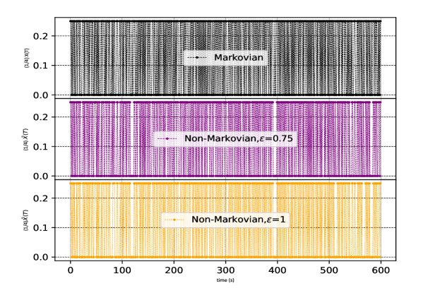
Figure 1: Realizations of the Markov process $X(T)$ with the joint probability distribution in equation (33), and the non-Markovian process $\tilde{X}(T)$ with the joint probability distribution in equation (37) for different values of the parameter $\varepsilon$. The probability vectors $\mathbf{p}(t_{3k-2})$ have been chosen as $(0.25,0.75)^{T}$ for all $k=1,2,3,\ldots$. The first two time steps of the realizations have been generated using the same random numbers since there is no difference between the Markovian and the non-Markovian process for the first two time steps. From these realizations, one finds the following numerical values: $\mu=0.575,\tilde{\mu}=0.585$ (for $\varepsilon=0.75$), $\tilde{\mu}=0.580$ (for $\varepsilon=1$), $\rm{Var}(X)=0.022,\rm{Var}(\tilde{X})=0.039$ (for $\varepsilon=0.75$), $\rm{Var}(\tilde{X})=0.050$ (for $\varepsilon=1$), which are in accordance with the analytical predictions within statistical error.

From equation (37), one can straightforwardly derive the modified transition matrix $\tilde{S}_{1}$ as

$$\tilde{S}_{1}=\begin{bmatrix}\varepsilon q_{1}&(1-\varepsilon)q_{1}+q_{2}\\ (1-\varepsilon)q_{1}+q_{2}&\varepsilon q_{1}\end{bmatrix}=q_{1}(\varepsilon I+(1-\varepsilon)S_{1})+q_{2}S_{1}.$$ (38)

It can be checked that the new process with the transition matrices $\{\tilde{Q}_{1}^{(1)},Q_{1}^{(2)},\tilde{S}_{1},R\}$ satisfies the necessary condition in equation (20). Moreover, the Chapman-Kolmogorov equation $L_{1}=\tilde{S}_{1}R$ is fulfilled, while the Markov condition in equation (27) is not. Therefore, the new process $\tilde{X}(T)$ is a P-divisible non-Markovian process. Similar to Feller’s example, while the random variables $\{\tilde{X}_{t_{1}},\tilde{X}_{t_{2}},\tilde{X}_{t_{3}}\}$ are pairwise independent, they are not mutually independent. We also note that $\tilde{S}_{1}$ depends on the initial probability as was argued by Hänggi and Thomas [9] and by McCauley.[6]

To get an idea of how the resulting P-divisible non-Markovian process differs from the original Markov process, we show some realizations in Figure 1 for different values of the parameter $\varepsilon$. The average value $\tilde{\mu}$ of $\tilde{X}(t)$ for all values of $\varepsilon$ is surprisingly equal to that of $X(t)$. However, the variance $Var(\tilde{X})$ of $\tilde{X}(t)$ is equal to $(1/9)((1+\varepsilon)q_{1}-q_{1}^{2})$, which differs from that of $X(t)$. For the initial probability, $\mathbf{p}(t_{1})=(0.25,0.75)^{T}$, it is equal to $0.041$ and $0.049$ for $\varepsilon=0.75$ and $1$ respectively. The difference between the Markovian and the non-Markovian processes in terms of variance can also be captured partially from the realizations in Figure 1 by observing the gaps around, for example, the time step $t=400$. The gaps can be interpreted as an impact of memory on future states.

As $\varepsilon\rightarrow 0$, the process approaches the original Markov process. On the other hand, the memory of the process increases by increasing $\varepsilon$, leading to an increase of the degree of non-Markovianity. In addition, it is noteworthy that the process reduces to the P-divisible non-Markovian process given by van Kampen in the limit $\varepsilon\rightarrow 1$ and for $\mathbf{p}(t_{1})=(0.5,0.5)^{T}$. Thus, we conclude that Markovian and P-divisible non-Markovian processes are essentially different from each other. Furthermore, considering also equation (36), this example suggests that a P-divisible non-Markovian process might arise from disturbing a certain Markov process. This disturbance induces memory effects in the process, but the memory only lasts for a short time and the process returns to its original Markovian evolution. The memory effect manifests itself in $\mathrm{Var}(\tilde{X})$ being greater than $\mathrm{Var}(X)$.

The two-state P-divisible non-Markovian process presented above might seem purely a mathematical artefact, but it has the potential to be applied to some physical problems. Below, we will present such an application.

IV.3 Physical model of the two-state P-divisible non-Markovian process

We consider a city with a population of $N$. Suppose a new epidemic arises in the city, and in compliance with regulations, everyone must wear a mask until a vaccine is developed. Fortunately, a vaccine is developed, and the city government plans a vaccination program with specific appointment times for the three doses. Then, the government announces that individuals who receive at least two vaccinations may remove their masks and resume normal activities and that those who have not yet received two vaccinations must continue to wear masks until the next vaccination schedule.

In such a model, depending on the first dose, some individuals might not take the third dose because two doses are enough to resume their normal life. Therefore, the memory of the first dose will affect receiving the third vaccine. In addition, there might be some people who are against vaccination, so they may resist getting vaccinated. The individual’s state of being vaccinated at each of three appointments can be represented with the state space $\mathbb{E}=\{0,1\}$, such that $0$ and $1$ correspond to the events ”not getting vaccinated” and ”getting vaccinated”, respectively. We assume that each individual is vaccinated independently of each other. Then, the vaccination process of each individual at the first schedule can be represented with the first triple steps, $\{\tilde{X}_{t_{1}},\tilde{X}_{t_{2}},\tilde{X}_{t_{3}}\}$, of the two-state P-divisible non-Markovian process given above conditioned on the following specific statements related to the memory of the first vaccination:

1. Each individual gets the first vaccination with the initial probability, $\mathbf{p}(t_{1})=(q_{1},q_{2})^{T}$.

2. Depending on vaccination status at one of the appointments, people are neutral against one of the other vaccines because they might think that they do not have to get vaccinated three times to be free of masks, and therefore, they might skip one of the vaccination appointments. We quantify this situation with the two-point conditional probabilities: $p(j,t_{3}\mid k,t_{2})=p(j,t_{3}\mid k,t_{1})=p(j,t_{2}\mid k,t_{1})=1/2$.

3. If an individual gets the first two vaccinations, they do not get the third one because they are free of masks: $p_{1\mid 2}(0,t_{3}\mid 1,t_{2};1,t_{1})=1$.

4. If an individual gets the first but not the second vaccination, they get the third one surely to be free of mask: $p_{1\mid 2}(1,t_{3}\mid 0,t_{2};1,t_{1})=1$.

5. If an individual does not get vaccinated at the first appointment, they do not also get vaccinated at the third appointment conditioned on the second vaccination with the following probabilities: $p_{1\mid 2}(0,t_{3}\mid 0,t_{2},0,t_{1})=\varepsilon$, $p_{1\mid 2}(0,t_{3}\mid 1,t_{2},0,t_{1})=1-\varepsilon$. Such an individual might be against vaccination at the beginning and later might change their opinion because of some reason, such as being informed about the benefits of vaccination.

The joint probability of the three vaccinations for each individual in the city whose individuals show the above characteristics can be reasonably represented by equation (37). Now, our question is as follows:

Question: How many people will be free of masks after the first three vaccinations?

According to the government announcement, those who have been vaccinated at least two times will be free of masks. Therefore, those individuals will be free of masks whose vaccination state matches with one of the following events: $(1,t_{3};1,t_{2};1,t_{1})$, $(0,t_{3};1,t_{2};1,t_{1})$, $(1,t_{3};0,t_{2};1,t_{1})$ and $(1,t_{3};1,t_{2};0,t_{1})$. Then, the number of individuals who are free of masks is

$$\begin{split}&N\big{(}p_{3}(1,t_{3};1,t_{2};1,t_{1})+p_{3}(0,t_{3};1,t_{2};1,t_{1})+p_{3}(1,t_{3};0,t_{2};1,t_{1})+p_{3}(1,t_{3};1,t_{2};0,t_{1})\big{)}\\ &=N\left(0+\frac{q_{2}}{2}+\frac{q_{2}}{2}+\frac{\varepsilon}{2}q_{1}\right)=N\left(q_{2}+\frac{\varepsilon}{2}q_{1}\right)=N(1-q_{1}(1-\varepsilon/2)).\end{split}$$ (39)

In this model, it seems that the memory parameter $\varepsilon$ refers to the situation of raising awareness in those individuals who have not been vaccinated at the first appointment. These individuals might be either those against vaccination or those who have decided not to take the vaccination according to the information given in items $2$ and $5$.

The number of unvaccinated individuals for the next schedule will be $N-N(1-q_{1}(1-\varepsilon/2))=Nq_{1}(1-\varepsilon/2)$. The vaccination process of these unvaccinated individuals for the next schedule can be represented by the second triple steps, $\{\tilde{X}_{t_{4}},\tilde{X}_{t_{5}},\tilde{X}_{t_{6}}\}$, of the two-state P-divisible non-Markovian process under the same conditions given above. However, the initial probability might be updated as $\mathbf{p}(t_{4})=(q_{1},q_{2})^{T}\rightarrow(q_{1}(1-\varepsilon/2),q_{2}+q_{1}\varepsilon/2)^{T}$ to take into account the effect of the memory on the unvaccinated individuals during the first vaccination process. Such a modification can be made if the government has recorded the vaccinated people in equation (39) during the first schedule and used this information to update the initial probability for the second schedule. We point out that this modification would change the mean value and the variance of the P-divisible non-Markovian processes because the equation $\mathbf{p}(t_{3k-2})=\mathbf{p}(t_{1})$ no longer holds for all $k=1,2,3,\ldots$.

We could also model the epidemic according to the Markov process whose joint probability is given by equation (33). In that case, there would not be any memory effect, $\varepsilon=0$. The number of individuals who were free of masks after the first schedule would be $N(1-q_{1})$, which is less than that of the non-Markovian case. The number of unvaccinated individuals for the next schedule would be $Nq_{1}$, which is greater than that of the non-Markovian case. A possible lesson we can take away from this example is that in bad cases like epidemics, raising people’s awareness affects the evolution of the case in time.

V Conclusion

P-divisibility is an essential property for the differential analysis of classical stochastic processes. For instance, the Kolmogorov forward and backward equations require the P-divisibility of the process.[5, 15] As has been stated in Corollary 1, we have established a necessary condition for the transition matrices of P-divisible stochastic processes within a finite sample space. It has some useful features and advantages as it provides a systematic way of constructing a P-divisible non-Markovian process from a given Markovian process. This approach is based on the (multipoint) memory transition matrices by which one can encode certain memory effects, as has been expressed by equation (36).

We have illustrated Corollary 1 by two examples in section IV. First, Feller’s example [4] has been shown to be a consistent P-divisible non-Markovian process. Therefore, in contrast to Feller, we have argued that P-divisible non-Markovian processes are not pathological, as they seem to arise by injecting short-term memory into certain Markov processes. In the second example and its application to the epidemic, we have illustrated this idea through our construction of the two-state P-divisible non-Markovian process utilizing the necessary condition in equation (20). The process is distinguished by a parameter $\varepsilon$, which characterizes the degree of non-Markovianity and can be measured in terms of the variance of the process.

Concluding, we have clarified that there are P-divisible non-Markovian processes which can be systematically constructed from certain Markov processes by taking into account so-called memory transition matrices describing the impact of memory effects.

Conflict of interest–The authors declare that they have no conflicts of interest.
References

References

- Snell [1997] J. Snell, “A Conversation with Joe Doob,” Stat. Sci. 12, 301 (1997).
- van Kampen [2007] N. G. van Kampen, Stochastic Processes in Physics and Chemistry, 3rd ed. (North Holland, Amsterdam, 2007) pp. 73–79.
- Lévy [1956] P. Lévy, “Processus semi-markovien,” Proc. Int. Congr. Math. 3, 416–426 (1956), it is available on https://www.mathunion.org/icm/proceedings.
- Feller [1959] W. Feller, “Non-markovian processes with semigroup property,” Ann. Math. Statist. 30, 1252 (1959).
- Feller [1970a] W. Feller, An Introduction to Probability Theory and Its Applications Vol.1, 3rd ed. (Wiley, New York, 1970) p. 471.
- McCauley [2012] J. McCauley, “Non-markov stochastic processes satisfying equations usually associated with a markov process,” Eur. Phys. J. Spec. Top. 204, 133 (2012).
- Orsingher, Ricciuti, and Toaldo [2018] E. Orsingher, C. Ricciuti, and B. Toaldo, “On semi-Markov processes and their Kolmogorov’s integro-differential equations,” J. Funct. Anal. 275, 830–868 (2018).
- Cinlar [2013] E. Cinlar, Introduction to Stochastic Processes, reprint ed. (Dover, New York, 2013).
- Hänggi and Thomas [1977] P. Hänggi and H. Thomas, “Time evolution, correlations, and linear response of non-markov processes,” Z. Physik B 26, 85 (1977).
- Vacchini et al. [2011] B. Vacchini, A. Smirne, E.-M. Laine, J. Piilo, and H.-P. Breuer, “Markovianity and non-markovianity in quantum and classical systems,” New J. Phys. 13, 093004 (2011).
- Chruściński, Kossakowski, and Rivas [2011] D. Chruściński, A. Kossakowski, and A. Rivas, “On measures of non-Markovianity: divisibility vs. backflow of information,” Phys. Rev. A 83, 052128 (2011).
- Wißmann, Vacchini, and Breuer [2015] S. Wißmann, B. Vacchini, and H.-P. Breuer, “Generalized trace distance measure connecting quantum and classical non-markovianity,” Phys. Rev. A 92, 042108 (2015).
- Note [1] We have presented here the modified version of the example which was explored by Feller on pages and of his book[5].
- Note [2] See the sixth example on p.79 of van Kampen’s book[2].
- Feller [1970b] W. Feller, An Introduction to Probability Theory and Its Applications Vol.2, 2nd ed. (Wiley, New York, 1970) pp. 290–356.