A Computationally Efficient Approach to False Discovery Rate Control and Power Maximisation via Randomisation and Mirror Statistic

Abstract

Simultaneously performing variable selection and inference in high-dimensional regression models is an open challenge in statistics and machine learning. The increasing availability of vast amounts of variables requires the adoption of specific statistical procedures to accurately select the most important predictors in a high-dimensional space, while controlling the False Discovery Rate (FDR) arising from the underlying multiple hypothesis testing. In this paper we propose the joint adoption of the Mirror Statistic approach to FDR control, coupled with outcome randomisation to maximise the statistical power of the variable selection procedure. Through extensive simulations we show how our proposed strategy allows to combine the benefits of the two techniques. The Mirror Statistic is a flexible method to control FDR, which only requires mild model assumptions, but requires two sets of independent regression coefficient estimates, usually obtained after splitting the original dataset. Outcome randomisation is an alternative to Data Splitting, that allows to generate two independent outcomes, which can then be used to estimate the coefficients that go into the construction of the Mirror Statistic. The combination of these two approaches provides increased testing power in a number of scenarios, such as highly correlated covariates and high percentages of active variables. Moreover, it is scalable to very high-dimensional problems, since the algorithm has a low memory footprint and only requires a single run on the full dataset, as opposed to iterative alternatives such as Multiple Data Splitting.

1 Introduction

Advances in data collection capabilities have allowed researchers to get access to thousands of features on multiple subjects in relatively short times. Examples are next-generation sequencing technologies that allow fast DNA and RNA sequencing and Nuclear Magnetic Resonance Spectroscopy used to identify metabolites. But also wearable personal devices that can measure several anthropometric variables and clinical outcomes of interests, such as blood pressure and blood glucose levels, continuously over time, thus producing a huge amount of fine-grained measurements. Moreover, it is now common to integrate these multiple input sources into a single study, and repeating these measurements over multiple time points, in a longitudinal fashion, in order to capture potentially relevant trends in the outcomes of interest, given some specific interventions or treatments.
The combination of all these factors generates an incredibly vast and complex set of features that researchers need to analyse with the goal of extracting and estimating the effects of only the most critical drivers related to the biological mechanism under study. This can be a daunting task, for at least two reasons: $1)$ the available sample size, e.g. the number of patients recruited in a cohort study, is very often much lower than the number of available features (high-dimensional problem). Therefore, standard statistical or machine learning models struggle to extract the underlying fundamental associations, due to model limitations. $2)$ even when a model can deal with a sample size lower than the number of features, the high probability of selecting false positive effects, caused by the underlying multiple hypothesis testing process, poses a serious threat to the validity of the analysis.
We address the first problem of variable selection by using all available features during the training process, building a statistical model that can automatically select the most relevant variables. This allows to retain the full interpretability about the effects of the covariates on the outcome of interest, in contrast with dimensionality reduction techniques such as Principal Component Analysis [AHT20]. In high-dimensional regression (or classification) problems, popular choices are the LASSO [Tib96], ElasticNet [ZH05], LARS [Efr+04] and SCAD [FL11], which provide efficient algorithms that scale well to a large number of features. Alternatives also exist in the Bayesian framework, where variable selection is performed through an appropriate choice of the prior distributions [OS09]. Popular choices are the two-group Spike and Slab prior distribution, which explicitly provide posterior probabilities of inclusion for each variable; and the one-group prior, such as the Laplace prior distribution, which shrinks coefficients toward zero, acting as a regularisation in a similar fashion to the $L_{1}$ penalty in the LASSO.
In addition to selecting only a subset of variables, in many applications to real data it is also essential to be able to make proper inference on the selected subset of features. This is essential to have a reliable estimate of the regression coefficients confidence intervals and to be able to control some form of error rate, such as the False Discovery Rate (FDR, [BH95]). However, simply proceeding with inference, after a data-dependent variable selection step, does not allow to perform valid post-selection inference, as explained in [Ber+13]. This is because data-driven variable selection procedures, such as the ones mentioned above, generate a model that is not deterministic and the straightforward application of classic approaches to inference, like Ordinary Least Squares, do not account for this additional randomness. Therefore, the estimated coefficients, and the corresponding confidence intervals will be biased, leading to a potential increase in erroneous classifications.
A number of methods exist to control error rates in multiple testing. [MB10] propose stability selection, as a method to control the number of False Discoveries in a LASSO regression setting. [Ber+13] takes a different approach, providing an analytical solution for the linear regression problem when using a LASSO penalty, formally accounting for the variable selection process at the inferential step, thus obtaining correct confidence intervals for the selected coefficients. [RBG22] provide a partial extension to the case of additive and linear mixed models, using Monte Carlo approximations, however the proposed solution is computationally intensive. Overall, this formal treatment is limited to simple cases, such as linear regression, and extensions are difficult.
[BC15], in their pioneering work, propose the knockoff filters procedure as a direct way to control the False Discovery Rate (FDR). The knockoff method works by augmenting the space of covariates, adding a perturbed version of each feature to the design matrix and performing variable selection on the new feature space. The authors provide an upper-bound estimate of the FDR and a new knockoff test statistic through which it is possible to control the FDR at any specific level. This approach, however, has some limitations, i.e. the knowledge of the joint distribution of the covariates is required to construct the knockoff filters and the procedure is limited to the case $n>p$. [Can+18] provide an extension to the high-dimensional scenarios, but still requires knowledge of the joint distribution of the covariates, which is not known in most real data applications.
Despite the limitations of the knockoff, the idea of feature perturbation has been successfully adopted in other works as a way to control FDR. [XZL21] develop the Gaussian Mirrors procedure which allows to control FDR without requiring any distributional assumption on the covariates. However, this approach is inefficient because it only evaluates one variable at a time. Using a similar approach, [Dai+22] develop the Mirror Statistic, by substituting the feature perturbation step with a two-steps procedure based on data splitting (DS). The first step being variable selection on a subset of the data and the second step being statistical inference on a second subset of data, independent of the first. This strategy allows to perform inference simultaneously on all variables and is therefore more efficient. One drawback of this approach is the loss of power caused by the reduced sample size available for the inference step (and similarly for the variable selection step). To mitigate this problem the authors propose a variation called Multiple Data Splitting (MDS), more akin to stability selection, showing increased power in simulations. Nevertheless, MDS is computationally much more costly, since the same procedure has to be repeated multiple times (at least $50$ according to the authors).

In this paper we propose to use the Mirror Statistic, but, instead of creating two independent sub-samples using data splitting, we borrow the idea of outcome randomisation from [TT18], where the authors propose a simple mechanism to create two independent sets of data by adding some random noise to the outcome, splitting more efficiently the original information available into two independent new pseudo-outcomes. The result is an increase in statistical power and a more computationally efficient algorithm. We provide a performance comparison via numerical experiments, replicating the results of [Dai+22] and extending the simulation scenarios to more challenging settings.
Throughout the article we use the following notation: RandMS to indicate our proposed model with outcome Randomisation plus Mirror Statistic, DS for single Data Splitting with Mirror Statistic, MDS for Multiple Data Splitting with Mirror Statistic. $S_{0}$ indicates the set of features with a true null coefficient and $S_{1}$ the set of features with a true non-null coefficient (active variables). X denotes the whole matrix of covariates, $\text{X}_{j}$ denotes column $j$ and $\boldsymbol{y}$ denotes the vector outcome. We make use of the terms variables, covariates and features interchangeably.
The remainder of the article is organized as follows. In Section 2 we review the methodology underlying FDR control via the Mirror Statistic and Data Splitting. We then introduce Randomisation and provide the algorithm for our proposed strategy. In Section 3 we show in detail the results of our simulations and the computational performance of the algorithm. In Section 4 we apply the proposed method to the selection of genes in a high-dimensional real-world study. Finally, in Section 5 we summarise our contributions, limitations and potential extensions of the method.

2 Methods

2.1 False Discovery Rate control

The False Discovery Rate has been introduced by [BH95] as a less conservative approach to False Positive error control compared to the Family-Wise Error Rate, which can be too restrictive when testing a large number of hypothesis. FDR is defined as the expectation of the False Discovery Proportion, defined as:

$$\text{FDR}=\mathbf{E}\left[\text{FDP}\right]=\mathbf{E}\left[\dfrac{\#\left\{j:j\in S_{0},j\in\hat{S}\right\}}{\#\left\{j:j\in\hat{S}\right\}\vee 1}\right]$$ (1)

where the expectation is taken with respect to the stochastic model selection procedure and the randomness in the data. $\hat{S}$ represents the set of all selected features.
[BH95] provides a correction method for the p-values so that a specific FDR level $\alpha$ can be achieved, under the assumption of independence of the p-values. Although some extensions exist that allow for some form of dependence [BY01], for many of the aforementioned algorithms in Section 1, p-values are not available at all (e.g. LASSO). Hence, the necessity of using methods that can achieve FDR control without explicitly calculating p-values, such as the Mirror Statistic (Eq. 2).

2.2 Data Splitting and Randomisation

The practice of splitting a given dataset into multiple smaller independent slices is common and the standard in most machine learning applications [Bis06], where, generally, a training, validation and testing set are generated from the original sample. While in machine learning, splitting is done to validate the prediction accuracy of a model, in classic statistical inference the same idea can be used to create valid inferential procedures. [Dai+22] use this strategy in order to control FDR via the test statistic Mirror Statistic, defined for variable $\text{X}_{j}$ as:

$$M_{j}=\text{sign}\left(\ \hat{\beta}^{(1)}_{j}\hat{\beta}^{(2)}_{j}\right)f\left(|\hat{\beta}^{(1)}_{j}|,|\hat{\beta}^{(2)}_{j}|\right)$$ (2)

where $f(|x|,|y|)$ is a non-negative and monotonically increasing function and $\hat{\beta}^{(1)}_{j}$ and $\hat{\beta}^{(2)}_{j}$ are two distinct estimates of the regression coefficient obtained on two independent subsets of the sample. The logic behind Eq. 2 is that for features that are relevant, the corresponding $M_{j}$ will get a positive relatively large value, because the two independent estimates, $\hat{\beta}^{(1)}_{j}$ and $\hat{\beta}^{(2)}_{j}$, will have concordant signs. Conversely, if the estimated coefficients have discordant signs, $M_{j}$ will always get a negative value and if the estimates are relatively small, meaning that probably the features are not relevant, then $M_{j}$ will be small as well.
Under the assumption that, for a feature $j\in S_{0}$, the sampling distribution of at least one of the two coefficients is symmetric around zero, then also $M_{j}$ will be symmetric around zero. This property, plus the Mirror Statistic construction, provides an upper bound on the number of false positives:

$$\#\left\{j\in S_{0}:M_{j}>t\right\}\approx\#\left\{j\in S_{0}:M_{j}<-t\right\}\leq\#\left\{j:M_{j}<-t\right\},\forall t>0$$ (3)

which can be directly used to approximate the False Discovery Proportion in Eq. 1.
As we can see from the definition, to use the Mirror Statistic estimator we need two independent sets of observations. Although data splitting is universally valid and straightforward to use, it comes at the cost of a much reduced sample size, which can have detrimental effects on the power of the statistical test and on the stability of the variable selection. To counteract this downside [Dai+22] propose MDS as a way to increase the power of the test statistic. MDS amounts to repeating multiple times the whole procedure of variable selection with simple DS and then aggregating the results. In simulations MDS seems to provide higher power; however, this improvement comes at the cost of a much higher computational burden and an additional uncertainty due to the choice of the aggregation strategy.
This is where Randomisation [TT18] offers an alternative way of distributing the available sample information and helps avoiding the randomness of the simple data splitting, creating two pseudo-independent sets, by perturbing the outcome with some random noise $W$. The general idea is to use a randomisation scheme through which we only allow ourselves to observe the outcome through $U\equiv u(Y,W)$ at the variable selection step, while at the inference step we only observe $V\equiv v(Y,W)$, with $V$ constructed to be independent of $U$.
Here we consider the case where the outcome of interest has a Normal distribution and whose mean is a function of some features X.

$$\boldsymbol{y}\sim\text{N}_{n}(\boldsymbol{\mu}=g(\text{X}),\sigma^{2}\text{I}_{n})$$ (4)

where $\text{I}_{n}$ is the $n$-dimensional identity matrix.
Given $\sigma^{2}$, or an estimate $\hat{\sigma}^{2}$, we can generate an $n$-dimensional vector of random Normal noise as $\boldsymbol{w}\sim\text{N}_{n}(\boldsymbol{0},\sigma^{2}\gamma\text{I}_{n})$, where the scalar $\gamma>0$ allows to distribute information for variable selection and inference ($\gamma=1$ corresponds to splitting data in half, while $\gamma<1$ places more information on $U$). Then, building $U=Y+W$, we have that $\boldsymbol{u}\sim\text{N}_{n}(\boldsymbol{\mu},\sigma^{2}(1+\gamma)\text{I}_{n})$ and $V=Y-\gamma^{-1}W$, with $\boldsymbol{v}\sim\text{N}_{n}(\boldsymbol{\mu},\sigma^{2}(1+\gamma^{-1})\text{I}_{n})$.
Randomisation can be interpreted as averaging information over all possible data splits of the same size. [TT18] show that for a Normally distributed outcome $\boldsymbol{y}$, randomisation guarantees a power that is always at least as high as data-splitting.
The complete inferential procedure is detailed in the following Algorithm:

Algorithm 1 Randomisation + Mirror Statistic

$\gamma$, $q$ (FDR target level), $\hat{\sigma}^{2}$

$\boldsymbol{w}\overset{IID}{\sim}\text{N}_{n}(\boldsymbol{0},\sigma^{2}\gamma\text{I}_{n})$

$\boldsymbol{u}=\boldsymbol{y}+\boldsymbol{w}$

$\boldsymbol{v}=\boldsymbol{y}-\gamma^{-1}\boldsymbol{w}$

Estimate regression coefficients $\boldsymbol{\hat{\beta}^{(u)}}$ and $\boldsymbol{\hat{\beta}^{(v)}}$ from $\boldsymbol{u}$ and $\boldsymbol{v}$ respectively.

Calculate MS $M_{j}$, $\forall j$, using Eq. 2.

Select the covariates $\text{X}_{j}$ for which ${M_{j}>\tau_{q}}$, where the threshold $\tau_{q}$ is

$$\tau_{q}=\text{min}\left\{t>0:\text{FDP}(t)=\dfrac{\#\left\{j:M_{j}<-t\right\}}{\#\left\{j:M_{j}>t\right\}\vee 1}\leq q\right\}$$

3 Simulations

To prove the effectiveness of our proposed approach we perform several simulations in multiple scenarios, comparing our method against DS and MDS.
We first repeat the simulations done in [Dai+22], to check whether we can achieve a similar performance to what was reported in the original paper. We then perform additional simulations under different scenarios, with the purpose of finding the limit of the approach, i.e. when the performance deteriorates too much, and to check in which situations our method can perform better than the alternatives.
The common strategy to all simulations is to perform variable selection with LASSO and inference with a standard linear model. For all simulations we set $f(a,b)=a+b$ in Eq. 2, as done in [Dai+22].
The metrics that we track are the False Discovery Rate (FDR) and the True Positive Rate (TPR, or Power). An ideal model selection will have a TPR close to $1$ for every level of FDR we wish to control for.

3.1 Replication of the simulations from the original paper with DS and MDS

The data for this scenario is generated using the following parameters:

• sample size, $n=800$

• number of covariates, $p=2000$

• number of non-zero coefficients, $p_{1}=50$, equivalent to $2.5\%$ of $p$

• covariates correlation, $\rho=\left\{0,0.2,0.4,0.5,0.6,0.8\right\}$

• regression coefficients signal strength, $\delta=\left\{3,4,5,6,7\right\}$

Throughout the paper the correlation coefficient $\rho$ represents the highest value from which the correlation matrix is built, following the structure defined in Eq. 5, unless otherwise specified.
The covariates are generated as independent random draws from a multivariate Normal distribution, $\boldsymbol{x}_{i}\sim\text{N}_{p}(\textbf{0},\Sigma)$, where the covariance $\Sigma$ is constructed as a diagonal Toeplitz matrix, with each block defined as:

$$\begin{bmatrix}1&\dfrac{(p^{\prime}-2)\rho}{(p^{\prime}-1)}&\dfrac{(p^{\prime}-3)\rho}{(p^{\prime}-1)}&\dots&\dfrac{\rho}{(p^{\prime}-1)}&0\\ \dfrac{(p^{\prime}-2)\rho}{(p^{\prime}-1)}&1&\dfrac{(p^{\prime}-2)\rho}{(p^{\prime}-1)}&\dots&\dfrac{2\rho}{(p^{\prime}-1)}&\dfrac{\rho}{(p^{\prime}-1)}\\ \vdots&&&\dots&&\vdots\\ 0&\dfrac{\rho}{(p^{\prime}-1)}&\dfrac{2\rho}{(p^{\prime}-1)}&\dots&\dfrac{(p^{\prime}-2)\rho}{(p^{\prime}-1)}&1\end{bmatrix}$$ (5)

where $p^{\prime}$ is the dimension of the block.
The regression coefficients are randomly generated from a Normal distribution with mean zero and standard deviation $\delta\sqrt{\log(p)/n}$.

Replicating the strategy used by [Dai+22] we first compare the performance of the three algorithms fixing the signal strength to $\delta=5$, varying the degree of correlation $\rho$, and then fixing the correlation to $\rho=0.5$ and varying the signal strength. MDS is run using $50$ replications of DS, as recommended by the authors.
$50$ independent replications are run for each combination. Here we show the boxplot of the results.
In Figures 3.1.1 and 3.1.2, top plots, we can observe some common patterns: $a)$ all three algorithms achieve, on average, FDR control at the nominal level of $0.1$; $b)$ MDS is always more conservative, achieving on average a lower FDR.
In the bottom plots, we show the TPR estimates: $a)$ MDS does not seem to be significantly better than the simple DS; $b)$ RandMS achieves a performance comparable to DS and MDS, with often higher (better) median values.
Something that was missing in the original paper is a mentioning about the variability of the estimates. Here we can see that when we account for that, MDS is not much superior to the simple DS, raising some doubts about the advantage of running a much slower and computationally intensive method, compared to a simpler one.

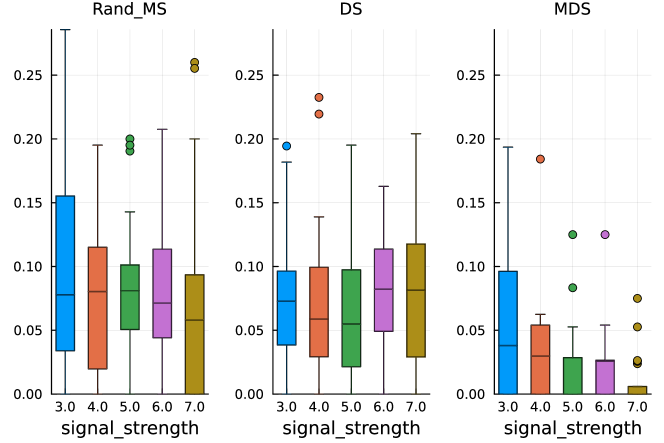
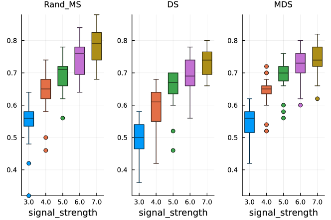
Figure 3.1.1: Paper replication study - $\rho=0.5$
Top: False Discovery Rate
Bottom: True Positive Rate

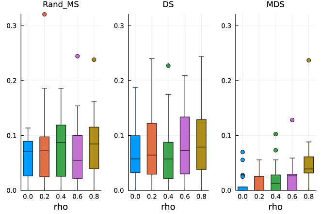
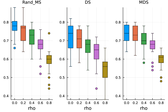
Figure 3.1.2: Paper replication study - signal strength $\delta=5$
Top: False Discovery Rate
Bottom: True Positive Rate

3.2 New simulations

We now concentrate on testing our method on new scenarios that were not covered in the original paper. We explore the performance in contexts with a higher correlation, near-ill conditioned covariance matrices, higher proportions of non-zero regression coefficients, non-block diagonal covariance matrices and regression coefficients sampled from a fixed known pool of values.

3.2.1 $\beta$ from fixed pool

The first additional scenario that we test is the situation where the regression coefficients $\boldsymbol{\beta}$ are not drawn from a distribution, as done in 3.1, but rather randomly sampled from a fixed known pool of values. For this simulation we sample $p$ values from the set $\left\{-1,-0.8,-0.5,0.5,0.8,1\right\}$.
Selecting the coefficients from a known set of values allows to better control and understand the variable selection capabilities of the algorithms, since the random draws from a Normal distribution will naturally be concentrated around the zero mean, making it more difficult to really understand which coefficients can actually be considered non-zero. This set of regression coefficients is used in all of the following simulations.
Keeping all the other simulation settings as before, we run the same simulations. From Figure 3.2.1 (top) we see that the median values and variability of FDR are very similar to the ones obtained before, validating the ability of the Mirror Statistic to control the FDR. On the other hand, the results for the TPR in Figure 3.2.1 (bottom) suggest that variable selection with fixed coefficients is somewhat easier, as expected, which is reflected in higher median TPR values, concentrated near $1$.
All three methods have a comparable performance, both in terms of FDR control and TPR, with the only exception of MDS, which has, on average, a lower TPR than DS and RandMS. This behaviour could be explained by the fact that MDS has a very conservative control over FDR, thus also ending up with a lower TPR.

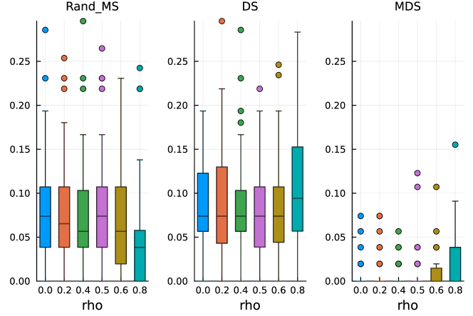
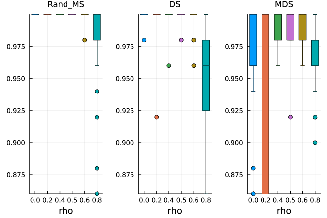
Figure 3.2.1: $\beta$ from fixed pool
Top: False Discovery Rate
Bottom: True Positive Rate

3.2.2 Higher percentages of non-zero coefficients

A natural question arises regarding whether DS, MDS and RandMS, can cope with a higher percentages of active variables, potentially highly correlated. To this end, we increase the complexity of the simulated data by increasing the percentage of active variables and allowing very high degrees of correlations across the covariates.
We start by increasing the percentage of active variables to $10\%$. From Figure 3.2.2 (top) we see that the FDR is still under control and MDS is conservative, as before. In Figure 3.2.2 (bottom) we can observe that RandMS is achieving a TPR always at least comparable to DS and MDS. Common to all three methods is the sharp decrease in TPR for higher correlation structures.

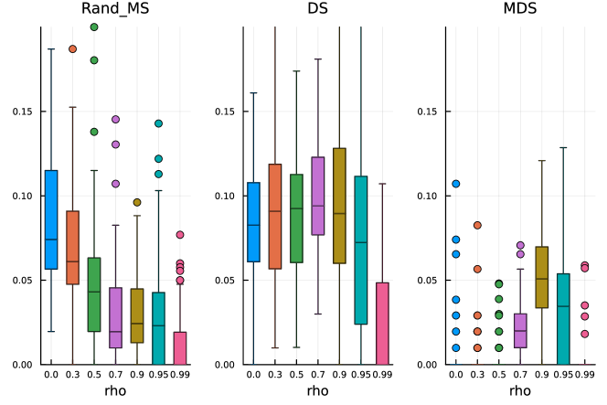
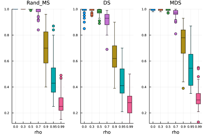
Figure 3.2.2: Active coefficients $10\%$
Top: False Discovery Rate
Bottom: True Positive Rate

By increasing the percentage of active variables to $20\%$, we can appreciate a sharper difference, at the advantage of RandMS, both in terms of FDR and TPR. In Figure 3.2.3 (top) we see that DS and MDS start to loose control over the FDR, in particular MDS is no longer as conservative as before. RandMS is still able to achieve the required FDR control at the pre-specified level.
In Figure 3.2.3 (bottom) we see that RandMS outperform the competitors in terms of TPR, in particular for correlations up to, and including, $0.5$. On the other hand, DS is totally unable to retain enough power.

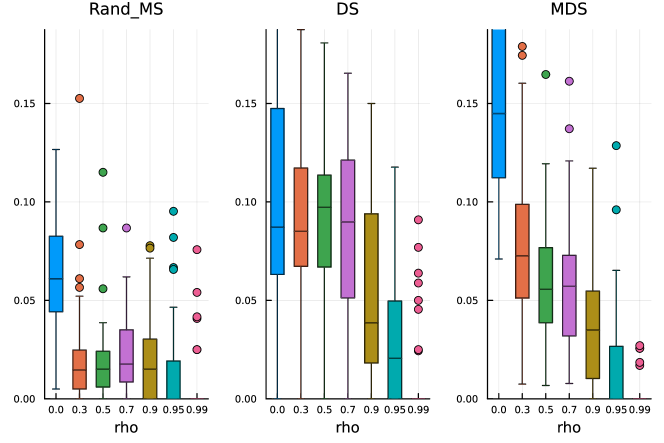
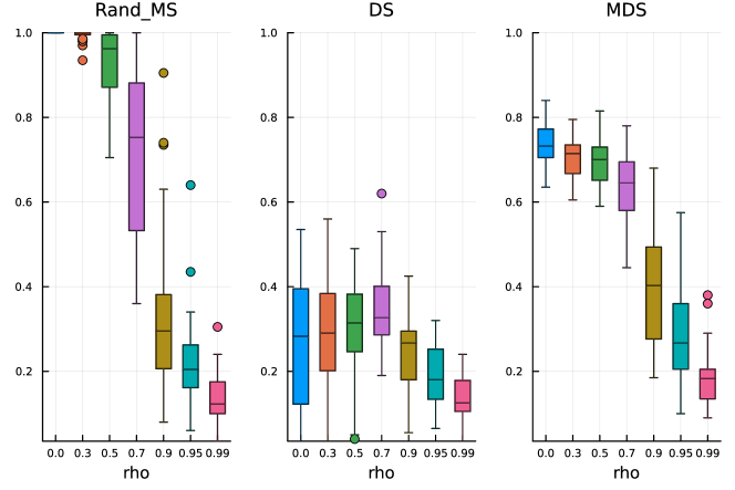
Figure 3.2.3: Active coefficients $20\%$
Top: False Discovery Rate
Bottom: True Positive Rate

Finally, setting the percentage of active variables to $30\%$, the difference is even more striking, again in favour of RandMS. Figures 3.2.4 (top) and 3.2.4 (bottom) show the results for FDR and TPR, respectively.

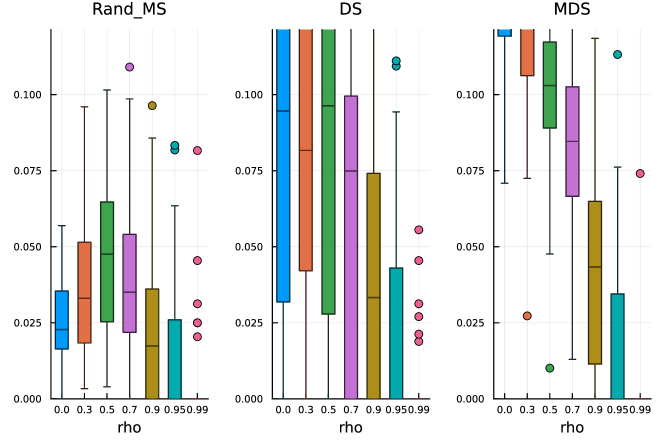
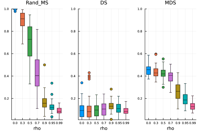
Figure 3.2.4: Active coefficients $30\%$
Top: False Discovery Rate
Bottom: True Positive Rate

3.2.3 Different covariance matrix structure

The next simulation is performed with covariates generated from a Normal distribution whose inverse covariance matrix is near ill-conditioned, meaning that the lowest eigenvalues of $\Sigma^{-1}$ are nearly $0$. This results in a more unstable data generation.
The covariance matrix $\Sigma$ is constructed starting from the identity matrix and changing only the first off-diagonal entries to be equal to some specified values, here denoted by $\rho\in{0.3,0.4,0.5}$. This covariance structure implies that

$$\text{corr}\left(X_{j},X_{j+1}\right) \neq 0$$

$$\text{corr}\left(X_{j},X_{j+2}\right) =0$$

In Figure 3.2.5 (top) we see that MDS is still conservative in terms of FDR, while DS and RandMS correctly control FDR at $10\%$. However, as we increase the percentage of active variables to $30\%$, Figure 3.2.6 (top), we see that MDS is not conservative anymore, while RandMS still works well.
In terms of TPR, the advantage of RandMS is more clear. Already with a percentage of active coefficients of $10\%$, Figure 3.2.5 (bottom), RandMS does a better job than DS and MDS, and, increasing that percentage to $30\%$, Figure 3.2.6 (bottom), RandMS totally outperforms the competitors.

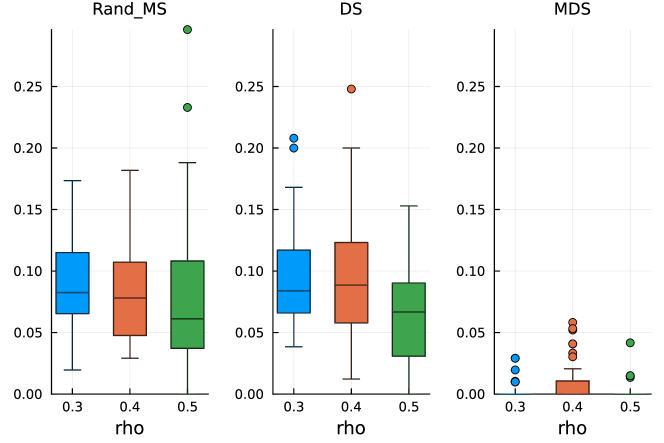
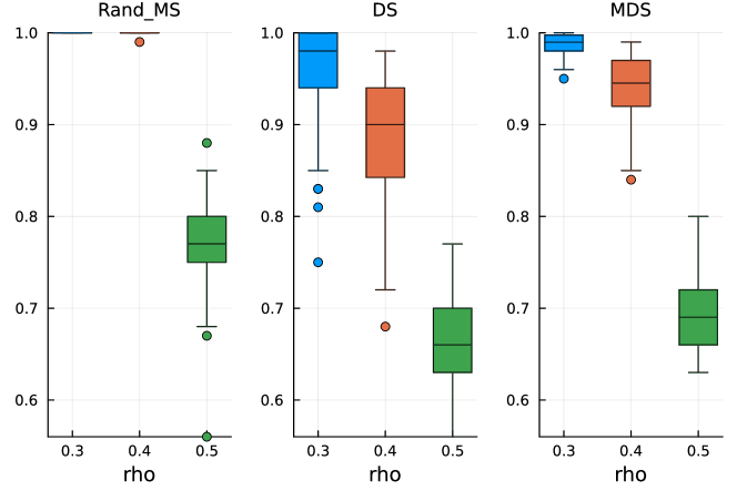
Figure 3.2.5: Ill conditioned covariance - active coefficients $10\%$
Top: False Discovery Rate
Bottom: True Positive Rate

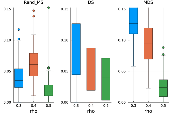
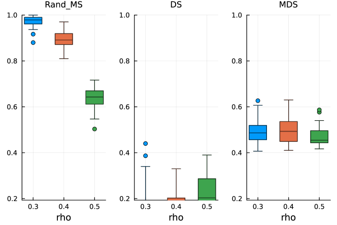
Figure 3.2.6: Ill conditioned covariance - active coefficients $30\%$
Top: False Discovery Rate
Bottom: True Positive Rate

3.2.4 Increasing $p$

Here we test the performance of RandMS with a higher number of covariates, $p=10000$, while keeping the sample size fixed at $n=800$. We repeat the simulations for different proportions of non-zero coefficients, from $0.003$ to $0.008$, which correspond to $p_{1}=30$ and $p_{1}=80$, respectively.
In Figure 3.2.7 we report the performance for $p_{1}=80$. RandMS is able to control the FDR at $0.1$ as required and is comparatively better than the other methods that show a higher variability. The TPR is much higher for RandMS up to, and including, a correlation factor of $0.7$, with TPR values close to $1$. The performance decreases for more extreme correlation levels as expected.

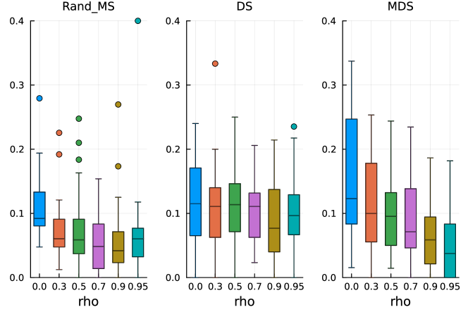
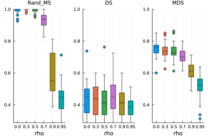
Figure 3.2.7: Block covariance matrix - $p=10000$ with $p_{1}=80$
Top: False Discovery Rate
Bottom: True Positive Rate

3.3 Computational performance

We run a benchmark simulation of the computational requirements for the proposed Randomisation plus Mirror Statistic method. The benchmark, as well as all other analysis, has been done in Julia ([Bez+17], version $1.9.3$) on a Lenovo ThinkPad machine, with Linux OS and equipped with a 13th Gen Intel® Core™ i5-1345U × 12 CPU.
In Figure 3.3.1 we show the average time for an increasing number of variables $p$, with a fixed number of active variables $p_{1}=10$, sample size $n=300$ and a block diagonal covariance matrix (where each block is a full matrix). Both time and memory requirements scale linearly with the number of variables; as an example, with $p=10000$ the time required to estimate the full model is about $4$ seconds, while the memory required is about $0.7$ GB.

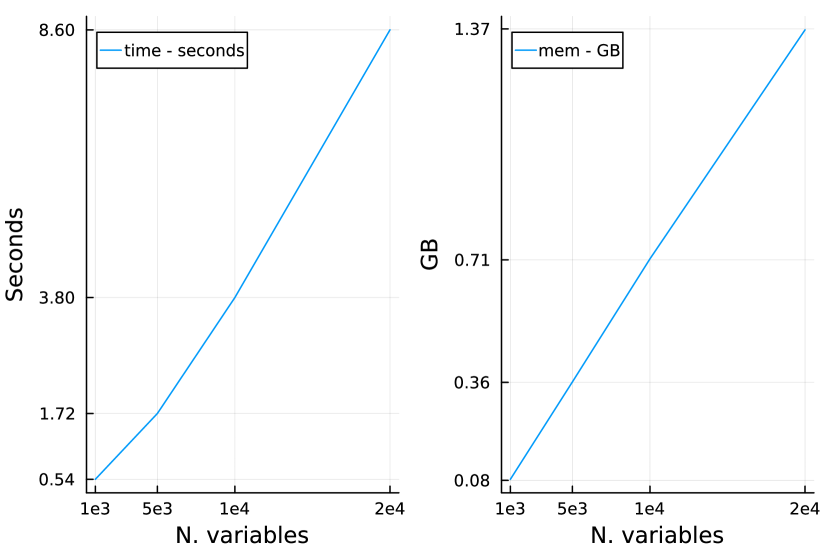
Figure 3.3.1: Computational benchmark of Randomisation with Mirror Statistic
Left: CPU time in seconds
Right: Memory footprint in Gigabytes

4 Real data application to the identification of genes regulating fasting triglyceride levels

Elevated serum triglyceride (TG) levels in blood are strongly associated with increased risk of cardiovascular diseases (CVD). Serum TG levels can be reduced by a healthy diet, but there are also large inter-individual variation in fasting TG levels. An improved understanding of this variation would be beneficial for CVD prevention. In this example, we are interested in relating fasting TG levels to gene expression through a linear regression model. We have data from the screening visit of a randomized controlled dietary intervention trial, presented in detail in [Ulv+16]. In this trial, gene expression was measured in Peripheral blood mononuclear cells (PBMC). These are immune system cells and because they are circulating cells, they are exposed to nutrients, metabolites and peripheral tissues and may therefore reflect whole-body health. We include all individuals from whom we have both PBMC gene expressions and fasting TG levels, in total 251 individuals. The outcome is the log measurement of blood triglycerides, while we use measurements from $13967$ genes expression as covariates ($HumanHT-12$ Expression BeadChips. Pre-processed gene expression probe level intensity values).
The log transformed triglyceride outcome is well approximated by a Normal distribution, while the gene expression data have been already preprocessed and are also well approximated by a Normal distribution.

We proceed to analyse the data with our proposed method, i.e. outcome Randomisation plus Mirror Statistic, in order to identify which genes could potentially contribute to the differences in TG levels. We use LASSO for variable selection on the randomised outcome $U$ and a standard linear regression model for the coefficients estimation on the randomised outcome $V$ (Algorithm 1); we set the randomisation parameter $\gamma=1$ and we choose $f(a,b)=a+b$ for the test statistic in Eq. 2. The FDR target level is set to $0.1$.
If we look only at the variable selection part of Algorithm 1 (i.e. LASSO), the number of selected genes is $30$, while only $2$ of those (plus the intercept) have been selected using the full RandMS algorithm. Both our selected genes can be linked to atherosclerosis, and thus, seem biologically plausible. MYLIP ($0.83\left[0.74,0.92\right]$) is related to TG level through LDL transport, while an over expression of ABCG1 ($0.89\left[0.80,0.98\right]$) results in increased efflux of cellular cholesterol to HDL, which has an inverse association with TG. The numbers in parentheses are the estimated multiplicative effect with the respective $95\%$ confidence interval in square brackets, thus an increased expression of both genes seem to have a positive effect on TG levels.

5 Discussion

We propose the adoption of outcome randomisation instead of Data Splitting, in combination with the Mirror Statistic, in order to effectively control the False Discovery Rate in high-dimensional linear regressions. Intuitively, Randomisation acts as information averaging and helps avoid the pitfalls of Data Splitting. When combined with the Mirror Statistic, it allows to correctly control the FDR at the target level, while providing higher power and a more computationally efficient algorithm.
Our extensive simulations show the superior performance compared to Data Splitting strategies, in various scenarios of increasing complexity. Even in very high-dimensional cases we can retain good scalability of the proposed method.
Finally, we perform a real data analysis, where the outcome of interest is blood triglyceride levels, and the covariates are gene expression data. The dimension of the covariates space, compared to the sample size, makes this problem a perfect example of high-dimensional linear regression. We use our method to perform variable selection and inference, with a target FDR of $10\%$. We are able to identify two genes, potentially responsible for the variation of triglyceride levels.
This extension is currently limited to Normally distributed outcomes, where randomisation takes a closed form analytical solution and the symmetry requirement of the regression coefficients to apply the Mirror Statistic is satisfied. It would be interesting to explore possible extensions to outcomes following arbitrary distributions and high-dimensional mixed models. [Lei+23] provides an extension of randomisation to distributions belonging to the exponential family, relying on the concept of conjugate distributions from Bayesian statistics. Their result could potentially be used, for example for a high-dimensional logistic regression. [Dai+23] extend the use of the Mirror Statistic to high-dimensional logistic regression, however, their method relies on the computationally expensive procedure of de-biasing the LASSO estimate, needed to satisfy the symmetry requirement to use the Mirror Statistic. Future efforts to combine these two extensions could be of practical interest. Another area of further improvement could be the adoption of different variable selection techniques in the first step of Algorithm 1. For example, substituting LASSO with a model that can better select highly correlated covariates, e.g. ElasticNet [ZH05].

Code availability

The code used to perform all the simulations, the real data analysis and the computational performance benchmark is available at https://github.com/marcoelba/SelectiveInference.

References

- [BH95] Yoav Benjamini and Yosef Hochberg “Controlling the False Discovery Rate: A Practical and Powerful Approach to Multiple Testing” In Journal of the Royal Statistical Society: Series B (Methodological) 57.1 Wiley, 1995, pp. 289–300 DOI: 10.1111/j.2517-6161.1995.tb02031.x
- [Tib96] Robert Tibshirani “Regression Shrinkage and Selection Via the Lasso” In Journal of the Royal Statistical Society: Series B (Methodological) 58.1 Wiley, 1996, pp. 267–288 DOI: 10.1111/j.2517-6161.1996.tb02080.x
- [BY01] Yoav Benjamini and Daniel Yekutieli “The control of the false discovery rate in multiple testing under dependency” In The Annals of Statistics 29.4 Institute of Mathematical Statistics, 2001 DOI: 10.1214/aos/1013699998
- [Efr+04] Bradley Efron, Trevor Hastie, Iain Johnstone and Robert Tibshirani “Least angle regression” In The Annals of Statistics 32.2 Institute of Mathematical Statistics, 2004 DOI: 10.1214/009053604000000067
- [ZH05] Hui Zou and Trevor Hastie “Regularization and Variable Selection Via the Elastic Net” In Journal of the Royal Statistical Society Series B: Statistical Methodology 67.2 Oxford University Press (OUP), 2005, pp. 301–320 DOI: 10.1111/j.1467-9868.2005.00503.x
- [Bis06] Christopher M. Bishop “Pattern recognition and machine learning”, Information science and statistics New York, NY: Springer, 2006
- [OS09] R. B. O’Hara and M. J. Sillanpää “A review of Bayesian variable selection methods: what, how and which” In Bayesian Analysis 4.1 Institute of Mathematical Statistics, 2009 DOI: 10.1214/09-ba403
- [MB10] Nicolai Meinshausen and Peter Bühlmann “Stability Selection” In Journal of the Royal Statistical Society Series B: Statistical Methodology 72.4 Oxford University Press (OUP), 2010, pp. 417–473 DOI: 10.1111/j.1467-9868.2010.00740.x
- [FL11] Jianqing Fan and Jinchi Lv “Nonconcave Penalized Likelihood With NP-Dimensionality” In IEEE Transactions on Information Theory 57.8 Institute of ElectricalElectronics Engineers (IEEE), 2011, pp. 5467–5484 DOI: 10.1109/tit.2011.2158486
- [Ber+13] Richard Berk et al. “Valid post-selection inference” In The Annals of Statistics 41.2 Institute of Mathematical Statistics, 2013 DOI: 10.1214/12-aos1077
- [BC15] Rina Foygel Barber and Emmanuel J. Candès “Controlling the false discovery rate via knockoffs” In The Annals of Statistics 43.5 Institute of Mathematical Statistics, 2015 DOI: 10.1214/15-aos1337
- [Ulv+16] Stine M. Ulven et al. “Exchanging a few commercial, regularly consumed food items with improved fat quality reduces total cholesterol and LDL-cholesterol: a double-blind, randomised controlled trial” In British Journal of Nutrition 116.8 Cambridge University Press (CUP), 2016, pp. 1383–1393 DOI: 10.1017/s0007114516003445
- [Bez+17] Jeff Bezanson, Alan Edelman, Stefan Karpinski and Viral B. Shah “Julia: A Fresh Approach to Numerical Computing” In SIAM Review 59.1 Society for Industrial & Applied Mathematics (SIAM), 2017, pp. 65–98 DOI: 10.1137/141000671
- [Can+18] Emmanuel Candès, Yingying Fan, Lucas Janson and Jinchi Lv “Panning for Gold: ‘Model-X’ Knockoffs for High Dimensional Controlled Variable Selection” In Journal of the Royal Statistical Society Series B: Statistical Methodology 80.3 Oxford University Press (OUP), 2018, pp. 551–577 DOI: 10.1111/rssb.12265
- [TT18] Xiaoying Tian and Jonathan Taylor “Selective inference with a randomized response” In The Annals of Statistics 46.2 Institute of Mathematical Statistics, 2018 DOI: 10.1214/17-aos1564
- [AHT20] Shaeela Ayesha, Muhammad Kashif Hanif and Ramzan Talib “Overview and comparative study of dimensionality reduction techniques for high dimensional data” In Information Fusion 59 Elsevier BV, 2020, pp. 44–58 DOI: 10.1016/j.inffus.2020.01.005
- [XZL21] Xin Xing, Zhigen Zhao and Jun S. Liu “Controlling False Discovery Rate Using Gaussian Mirrors” In Journal of the American Statistical Association 118.541 Informa UK Limited, 2021, pp. 222–241 DOI: 10.1080/01621459.2021.1923510
- [Dai+22] Chenguang Dai, Buyu Lin, Xin Xing and Jun S. Liu “False Discovery Rate Control via Data Splitting” In Journal of the American Statistical Association Informa UK Limited, 2022, pp. 1–18 DOI: 10.1080/01621459.2022.2060113
- [RBG22] David Rügamer, Philipp F.M. Baumann and Sonja Greven “Selective inference for additive and linear mixed models” In Computational Statistics & Data Analysis 167 Elsevier BV, 2022, pp. 107350 DOI: 10.1016/j.csda.2021.107350
- [Dai+23] Chenguang Dai, Buyu Lin, Xin Xing and Jun S. Liu “A Scale-Free Approach for False Discovery Rate Control in Generalized Linear Models” In Journal of the American Statistical Association 118.543 Informa UK Limited, 2023, pp. 1551–1565 DOI: 10.1080/01621459.2023.2165930
- [Lei+23] James Leiner, Boyan Duan, Larry Wasserman and Aaditya Ramdas “Data fission: splitting a single data point” In Journal of the American Statistical Association Informa UK Limited, 2023, pp. 1–22 DOI: 10.1080/01621459.2023.2270748