Analysis of the isospin eigenstate $\bar{D}\Sigma_{c}$, $\bar{D}^{*}\Sigma_{c}$, and $\bar{D}\Sigma_{c}^{*}$ pentaquarks by their electromagnetic properties

Abstract

To shed light on the nature of the controversial and not yet fully understood exotic states, we are carrying out a systematic study of their electromagnetic properties. The magnetic moment of a hadron state is as fundamental a dynamical quantity as its mass and contains valuable information on the deep underlying structure. In this study, we use the QCD light-cone sum rule to extract the magnetic moments of the $\mathrm{P_{c}(4312)}$, $\mathrm{P_{c}(4380)}$, and $\mathrm{P_{c}(4440)}$ pentaquarks by considering them as the molecular picture with spin-parity $\mathrm{J^{P}=\frac{1}{2}^{-}}$, $\mathrm{J^{P}=\frac{3}{2}^{-}}$, and $\mathrm{J^{P}=\frac{3}{2}^{-}}$, respectively. We define the isospin of the interpolating currents of these states, which is the key to solving the puzzle of the hidden-charm pentaquark states, in order to make these analyses more precise and reliable. We have compared our results with other theoretical predictions that could be a useful complementary tool for the interpretation of the hidden-charm pentaquark sector, and we observe that they are not in mutual agreement with each other. We have also calculated higher multipole moments for spin-3/2 $\bar{D}^{*}\Sigma_{c}$ and $\bar{D}\Sigma_{c}^{*}$ pentaquarks, indicating a non-spherical charge distribution.

I Introduction

In recent years, significant experimental progress has been made in the study of exotic hadrons, in particular in the observation of pentaquark states with hidden-charms, which has led to a great deal of interest in the study of pentaquarks. In 2015, two pentaquark states, named $\mathrm{P_{c}(4380)}$ and $\mathrm{P_{c}(4450)}$, were discovered by the LHCb Collaboration in the $J/\psi\,p$ invariant mass distribution of the $\Lambda_{b}\rightarrow J/\psi\,p\,K$ decay [1]. Four years later, with the inclusion of additional data, it was discovered that the $\mathrm{P_{c}(4450)}$ pentaquark state is composed of two narrow overlapping peaks, $\mathrm{P_{c}(4440)}$, and $\mathrm{P_{c}(4457)}$. Furthermore, a new narrow state, the $\mathrm{P_{c}(4312)}$, has been reported [2]. Note that the $\mathrm{\mathrm{P_{c}}(4380)}$ pentaquark state could neither be confirmed nor refuted in the updated analysis. In 2020 the LHCb Collaboration announced the first observation of the hidden-charm pentaquark state with strangeness, named $\mathrm{P_{cs}(4459)}$ [3]. The LHCb Collaboration announced recently also the discovery of two new narrow hidden-charm strange pentaquark states, $\mathrm{P_{cs}(4338)}$, with minimal quark content ($c\bar{c}uds$) [4]. The measured masses and widths of the four $c\bar{c}uud$ pentaquark states are

$$\rm{P_{c}(4312)}:M=4311.9\pm 0.7^{+6.8}_{-0.6}\,\rm{MeV}\,,\,\,\,\Gamma=9.8\pm 2.7^{+3.7}_{-4.5}\,\rm{MeV}\,,$$

$$\rm{P_{c}(4380)}:M=4380\pm 8.0\pm 29\,\rm{MeV}\,,\,\,\,\,\,\Gamma=205\pm 18\pm 86\,\rm{MeV}\,,$$

$$\rm{P_{c}(4440)}:M=4440.3\pm 1.3^{+4.1}_{-4.7}\,\rm{MeV}\,,\,\,\,\Gamma=20.6\pm 4.9^{+8.7}_{-10.1}\,\rm{MeV}\,,$$

$$\rm{P_{c}(4457)}:M=4457.3\pm 0.6^{+4.1}_{-1.7}\,\rm{MeV}\,,\,\,\,\Gamma=6.4\pm 2.0^{+5.7}_{-1.9}\,\rm{MeV}\,.$$ (1)

The discovery of the aforementioned pentaquarks immediately stimulated discussion of their properties and internal structure. Systematic study of their internal structure and nature can be a major step forward in our understanding of the non-perturbative behavior of the strong interaction. Hence, there have been a large number of theoretical studies trying to determine their masses, radiative decays, magnetic moments, and their production rates in the $\Lambda_{b}$ decay or the inclusive processes. Further discussions on the progress of the observed and possible pentaquarks and the other exotic states can be found in Refs. [5, 6, 7, 8, 9, 10, 11, 12, 13, 14, 15, 16, 17, 18, 19, 20], both in theory and experiment. However, despite all efforts, the true nature of these states remains one of the most important and challenging problems in hadron physics. As a result, further theoretical and experimental studies are needed to shed light on the nature of these and other exotic states.

The electromagnetic properties of the pentaquark states have not received much attention, though the mass spectra, production mechanisms, and decay behavior of the pentaquark states have received a great deal of attention from both theoretical and experimental sides [21, 22, 23, 24, 25, 26, 27, 28, 29, 30, 31, 32, 33, 34, 35, 36]. The magnetic moment is another observable parameter that may provide important information about the quark-gluon structure of hadrons and their fundamental nature and underlying dynamics. The magnetic moments of pentaquarks are a measure of their ability to interact with magnetic fields, and they are a prominent property for understanding the behavior of these states. In the electro- or photo-production of pentaquarks, different magnetic moments have an effect on both the differential and total cross-sections. Therefore, it is clear that a determination of the magnetic moments of the pentaquark states is extremely important to verify their nature. Motivated by this, in this study, we investigate the magnetic moments of the $\mathrm{P_{c}(4312)}$, $\mathrm{P_{c}(4380)}$, and $\mathrm{P_{c}(4440)}$ pentaquarks, assuming that these pentaquark states are $\bar{D}\Sigma_{c}$, $\bar{D}^{*}\Sigma_{c}$, and $\bar{D}\Sigma_{c}^{*}$ molecular states with spin-parity $\mathrm{J^{P}=\frac{1}{2}^{-}}$, $\mathrm{J^{P}=\frac{3}{2}^{-}}$, and $\mathrm{J^{P}=\frac{3}{2}^{-}}$, respectively. To make these analyses more precise and reliable, we define the isospin of the interpolating currents of these states, which is the key to solving the puzzle of the $\mathrm{P_{c}}$ states. Thanks to this, these interpolating currents couple potentially to the color singlet-singlet type $\mathrm{P_{c}}$ states rather than to the meson-baryon scattering states or thresholds. We should mention here that it is possible to study the magnetic moment of the $\mathrm{P_{c}(4457)}$ state as a $\bar{D}^{*}\Sigma_{c}^{*}$ molecular state. However, since the $\bar{D}^{*}\Sigma_{c}^{*}$ state is a spin-5/2 state, it can cause some additional complications in the calculations, which can affect the reliability of the analysis. Therefore, the magnetic moment of the $\bar{D}^{*}\Sigma_{c}^{*}$ state presents additional challenges and is beyond the scope of the present study. The magnetic moments belong to the non-perturbative regime of QCD and hence, a reliable non-perturbative method is needed to evaluate these physical observables. The QCD light-cone sum rule is one of the most efficient tools for the calculation of non-perturbative parameters [37, 38, 39].

The present work is organized as follows. In Sec. II, we obtain the QCD light-cone sum rules for isospin eigenstate $\bar{D}\Sigma_{c}$, $\bar{D}^{*}\Sigma_{c}$, and $\bar{D}\Sigma_{c}^{*}$ pentaquarks. The numerical analysis together with the discussion is presented in Sec. III. The last section is reserved for the summary. In the Appendix, we list the explicit expressions obtained for the magnetic moment of the $\bar{D}\Sigma_{c}$ pentaquark state with isospin-1/2.

II Electromagnetic properties of the isospin eigenstate $\bar{D}\Sigma_{c}$, $\bar{D}^{*}\Sigma_{c}$, and $\bar{D}\Sigma_{c}^{*}$ pentaquarks within the QCD light-cone sum rules

The initial attempt to study the magnetic moments of the spin-1/2 and spin-3/2 pentaquark states (hereafter referred to as $\mathrm{P_{c}}$ and $\mathrm{P_{c}^{*}}$, respectively) by QCD light-cone sum rules is to introduce the following correlation functions,

$$\Pi(p,q) =i\int d^{4}xe^{ip\cdot x}\langle 0|T\left\{J^{\mathrm{P_{c}}}(x)\bar{J}^{\mathrm{P_{c}}}(0)\right\}|0\rangle_{\gamma}\,,$$ (2)

$$\Pi_{\mu\nu}(p,q) =i\int d^{4}xe^{ip\cdot x}\langle 0|T\left\{J_{\mu}^{\mathrm{P_{c}^{*}}}(x)\bar{J}_{\nu}^{\mathrm{P_{c}^{*}}}(0)\right\}|0\rangle_{\gamma}\,,$$ (3)

where $T$ is the time ordered product, the $\gamma$ is the weak external electromagnetic field. The $J^{\mathrm{P_{c}}}(x)$ and $\mathrm{J^{P^{*}_{c}}}(x)$ are the interpolating currents for the spin-$1/2^{-}$ and spin-$3/2^{-}$ states, respectively. These interpolating currents are required for further analysis and are listed as follows

$$J^{\bar{D}\Sigma_{c}}(x) =\frac{1}{\sqrt{3}}\mid\bar{D}^{0}\Sigma_{c}^{+}\rangle\,\mp\sqrt{\frac{2}{3}}\mid\bar{D}^{-}\Sigma_{c}^{++}\rangle=\frac{1}{\sqrt{3}}\big{[}\bar{c}^{d}(x)i\gamma_{5}u^{d}(x)\big{]}\big{[}\varepsilon^{abc}u^{a^{T}}(x)C\gamma_{\alpha}d^{b}(x)\gamma^{\alpha}\gamma_{5}c^{c}(x)\big{]}$$

$$\mp\sqrt{\frac{2}{3}}\big{[}\bar{c}^{d}(x)i\gamma_{5}d^{d}(x)\big{]}\big{[}\varepsilon^{abc}u^{a^{T}}(x)C\gamma_{\alpha}u^{b}(x)\gamma^{\alpha}\gamma_{5}d^{c}(x)\big{]}\,,$$ (4)

$$J_{\mu}^{\bar{D}\Sigma_{c}^{*}}(x) =\frac{1}{\sqrt{3}}\mid\bar{D}^{0}\Sigma_{c}^{+*}\rangle\,\mp\sqrt{\frac{2}{3}}\mid\bar{D}^{-}\Sigma_{c}^{*++}\rangle=\frac{1}{\sqrt{3}}\big{[}\bar{c}^{d}(x)i\gamma_{5}u^{d}(x)\big{]}\big{[}\varepsilon^{abc}u^{a^{T}}(x)C\gamma_{\mu}d^{b}(x)c^{c}(x)\big{]}$$

$$\mp\sqrt{\frac{2}{3}}\big{[}\bar{c}^{d}(x)i\gamma_{5}d^{d}(x)\big{]}\big{[}\varepsilon^{abc}u^{a^{T}}(x)C\gamma_{\mu}u^{b}(x)d^{c}(x)\big{]}\,,$$ (5)

$$J_{\mu}^{\bar{D}^{*}\Sigma_{c}}(x) =\frac{1}{\sqrt{3}}\mid\bar{D}^{*0}\Sigma_{c}^{+}\rangle\,\mp\sqrt{\frac{2}{3}}\mid\bar{D}^{*-}\Sigma_{c}^{++}\rangle=\frac{1}{\sqrt{3}}\big{[}\bar{c}^{d}(x)\gamma_{\mu}u^{d}(x)\big{]}\big{[}\varepsilon^{abc}u^{a^{T}}(x)C\gamma_{\alpha}d^{b}(x)\gamma^{\alpha}\gamma_{5}c^{c}(x)\big{]}$$

$$\mp\sqrt{\frac{2}{3}}\big{[}\bar{c}^{d}(x)\gamma_{\mu}d^{d}(x)\big{]}\big{[}\varepsilon^{abc}u^{a^{T}}(x)C\gamma_{\alpha}u^{b}(x)\gamma^{\alpha}\gamma_{5}d^{c}(x)\big{]}\,,$$ (6)

where $a$, $b$, $c$ and $d$ are color indexes, and $C$ stands for the charge conjugation operator. As can be seen, $"\mp"$ appears in the explicit form of the interpolating currents written above. If the sign between these currents is minus, it couples to the isospin-1/2 states, while if it is plus, it couples to the isospin-3/2 states. As a result, in this study, the magnetic moments of both the isospin-1/2 states and the isospin-3/2 hidden-charm pentaquark states are determined.

In the hadronic representation, after inserting the full sets of hadronic states with the same quantum numbers as the interpolating currents and carrying out the Fourier integration over x, we acquire

$$\Pi^{Had}(p,q) =\frac{\langle 0\mid J^{\mathrm{P_{c}}}(x)\mid{\mathrm{P_{c}}}(p,s)\rangle}{[p^{2}-m_{\mathrm{P_{c}}}^{2}]}\langle{\mathrm{P_{c}}}(p,s)\mid{\mathrm{P_{c}}}(p+q,s)\rangle_{\gamma}\frac{\langle{\mathrm{P_{c}}}(p+q,s)\mid\bar{J}^{\mathrm{P_{c}}}(0)\mid 0\rangle}{[(p+q)^{2}-m_{\mathrm{P_{c}}}^{2}]}+\cdots,$$ (7)

$$\Pi^{Had}_{\mu\nu}(p,q) =\frac{\langle 0\mid J_{\mu}^{\mathrm{P_{c}^{*}}}(x)\mid{\mathrm{P_{c}^{*}}}(p,s)\rangle}{[p^{2}-m_{{\mathrm{P_{c}^{*}}}}^{2}]}\langle{\mathrm{P_{c}^{*}}}(p,s)\mid{\mathrm{P_{c}^{*}}}(p+q,s)\rangle_{\gamma}\frac{\langle{\mathrm{P_{c}^{*}}}(p+q,s)\mid\bar{J}_{\nu}^{\mathrm{P_{c}^{*}}}(0)\mid 0\rangle}{[(p+q)^{2}-m_{{\mathrm{P_{c}^{*}}}}^{2}]}+\cdots.$$ (8)

For further calculations, the matrix elements in Eqs. (7) and (8) are required and are written regarding the hadronic parameters as follows,

$$\langle 0\mid J^{\mathrm{P_{c}}}(x)\mid{\mathrm{P_{c}}}(p,s)\rangle= \lambda_{\mathrm{P_{c}}}\gamma_{5}\,u(p,s),$$ (9)

$$\langle{\mathrm{P_{c}}}(p+q,s)\mid\bar{J}^{\mathrm{P_{c}}}(0)\mid 0\rangle= \lambda_{\mathrm{P_{c}}}\gamma_{5}\,\bar{u}(p+q,s),$$ (10)

$$\langle{\mathrm{P_{c}}}(p,s)\mid{\mathrm{P_{c}}}(p+q,s)\rangle_{\gamma} =\varepsilon^{\mu}\,\bar{u}(p,s)\bigg{[}\big{[}F_{1}(q^{2})+F_{2}(q^{2})\big{]}\gamma_{\mu}+F_{2}(q^{2})\frac{(2p+q)_{\mu}}{2m_{\mathrm{P_{c}}}}\bigg{]}\,u(p+q,s),$$ (11)

$$\langle 0\mid J_{\mu}^{\mathrm{P_{c}^{*}}}(x)\mid{\mathrm{P_{c}^{*}}}(p,s)\rangle =\lambda_{{\mathrm{P_{c}^{*}}}}u_{\mu}(p,s),$$ (12)

$$\langle{\mathrm{P_{c}^{*}}}(p+q,s)\mid\bar{J}_{\nu}^{\mathrm{P_{c}^{*}}}(0)\mid 0\rangle =\lambda_{{\mathrm{P_{c}^{*}}}}\bar{u}_{\nu}(p+q,s),$$ (13)

$$\langle{\mathrm{P_{c}^{*}}}(p,s)\mid{\mathrm{P_{c}^{*}}}(p+q,s)\rangle_{\gamma} =-e\bar{u}_{\mu}(p,s)\bigg{[}F_{1}(q^{2})g_{\mu\nu}\varepsilon\!\!\!/-\frac{1}{2m_{{\mathrm{P_{c}^{*}}}}}\Big{[}F_{2}(q^{2})g_{\mu\nu}+F_{4}(q^{2})\frac{q_{\mu}q_{\nu}}{(2m_{{\mathrm{P_{c}^{*}}}})^{2}}\Big{]}\varepsilon\!\!\!/q\!\!\!/$$

$$+F_{3}(q^{2})\frac{1}{(2m_{{\mathrm{P_{c}^{*}}}})^{2}}q_{\mu}q_{\nu}\varepsilon\!\!\!/\bigg{]}u_{\nu}(p+q,s),$$ (14)

where $F_{i}$’s are the Lorentz invariant form factors, the $u(p,s)$, $u(p+q,s)$ and $\lambda_{{\mathrm{P_{c}}}}$ are the spinors and residue of the $\mathrm{P_{c}}$ state, respectively, and; the $u_{\mu}(p,s)$, $u_{\nu}(p+q,s)$ and $\lambda_{{\mathrm{P_{c}^{*}}}}$ are the spinors and residue of the $\mathrm{P_{c}^{*}}$ state, respectively.

Combining the above equations, and summing over spins, we obtain the following expressions for the correlation functions of the hadronic representation:

$$\Pi^{Had}(p,q)= \lambda^{2}_{\mathrm{P_{c}}}\gamma_{5}\frac{\Big{(}p\!\!\!/+m_{\mathrm{P_{c}}}\Big{)}}{[p^{2}-m_{{\mathrm{P_{c}}}}^{2}]}\varepsilon^{\mu}\bigg{[}\big{[}F_{1}(q^{2})+F_{2}(q^{2})\big{]}\gamma_{\mu}+F_{2}(q^{2})\,\frac{(2p+q)_{\mu}}{2m_{\mathrm{P_{c}}}}\bigg{]}\gamma_{5}\frac{\Big{(}p\!\!\!/+q\!\!\!/+m_{\mathrm{P_{c}}}\Big{)}}{[(p+q)^{2}-m_{{\mathrm{P_{c}}}}^{2}]},$$ (15)

$$\Pi^{Had}_{\mu\nu}(p,q) =\frac{\lambda_{{}_{{\mathrm{P_{c}^{*}}}}}^{2}}{[(p+q)^{2}-m_{{}_{{\mathrm{P_{c}^{*}}}}}^{2}][p^{2}-m_{{}_{{\mathrm{P_{c}^{*}}}}}^{2}]}\bigg{[}g_{\mu\nu}p\!\!\!/\varepsilon\!\!\!/q\!\!\!/\,F_{1}(q^{2})-m_{{\mathrm{P_{c}^{*}}}}g_{\mu\nu}\varepsilon\!\!\!/q\!\!\!/\,F_{2}(q^{2})-\frac{F_{3}(q^{2})}{4m_{{\mathrm{P_{c}^{*}}}}}q_{\mu}q_{\nu}\varepsilon\!\!\!/q\!\!\!/$$

$$-\frac{F_{4}(q^{2})}{4m_{{\mathrm{P_{c}^{*}}}}^{3}}(\varepsilon.p)q_{\mu}q_{\nu}p\!\!\!/q\!\!\!/+\cdots\bigg{]}.$$ (16)

In order to calculate the magnetic form factor, $F_{M}(Q^{2})(G_{M}(Q^{2})$, of these pentaquark states, these form factors must be written in terms of the form factors $F_{i}(Q^{2})$, and these expressions are given as follows

$$F_{M}(q^{2}) =F_{1}(q^{2})+F_{2}(q^{2}),$$ (17)

$$G_{M}(q^{2}) =\left[F_{1}(q^{2})+F_{2}(q^{2})\right](1+\frac{4}{5}\lambda)-\frac{2}{5}\left[F_{3}(q^{2})\right]+\left[F_{4}(q^{2})\right]\lambda\left(1+\lambda\right),$$ (18)

where $F_{M}(q^{2})$ and $G_{M}(q^{2})$ are magnetic form factor for spin-1/2 and spin-3/2 states, respectively and; $\lambda=-\frac{q^{2}}{4m^{2}_{{\mathrm{P_{c}^{*}}}}}$. Using the above expressions, we can obtain the electromagnetic form factors of these pentaquarks. However, since we are dealing with a real photon ($q^{2}=0$), we can obtain these form factors in terms of the magnetic moment, and their explicit expressions are as follows

$$\mu_{\mathrm{P_{c}}} =\frac{e}{2\,m_{\mathrm{P_{c}}}}\,F_{M}(0),$$ (19)

$$\mu_{{\mathrm{P_{c}^{*}}}} =\frac{e}{2m_{{\mathrm{P_{c}^{*}}}}}G_{M}(0).$$ (20)

On the QCD side, the correlation function is achieved in the deep Euclidean region by operator product expansion (OPE). To proceed, we should derive the correlation function employing the light and heavy quark propagators and the distribution amplitudes of the photon. Consequently, the results of the contractions for the $\bar{D}\Sigma_{c}$, $\bar{D}^{*}\Sigma_{c}$, and $\bar{D}\Sigma_{c}^{*}$ pentaquarks are listed as follows

$$\Pi^{\rm{QCD}-\mathrm{\bar{D}\Sigma_{c}}}(p,q) =\frac{i}{3}\varepsilon^{abc}\varepsilon^{a^{\prime}b^{\prime}c^{\prime}}\,\int d^{4}x\,e^{ip\cdot x}$$

$$\langle 0\mid\Big{\{}\mbox{Tr}\Big{[}\gamma_{5}S_{u}^{dd^{\prime}}(x)\gamma_{5}S_{c}^{d^{\prime}d}(-x)\Big{]}\mbox{Tr}\Big{[}\gamma_{\alpha}S_{d}^{bb^{\prime}}(x)\gamma_{\beta}\widetilde{S}_{u}^{aa^{\prime}}(x)\Big{]}(\gamma^{\alpha}\gamma_{5}S_{c}^{cc^{\prime}}(x)\gamma_{5}\gamma^{\beta})$$

$$\mp\mbox{Tr}\Big{[}\gamma_{5}S_{u}^{da^{\prime}}(x)\gamma_{\beta}\widetilde{S}_{d}^{bb^{\prime}}(x)\gamma_{\alpha}S_{u}^{ad^{\prime}}\gamma_{5}(x)S_{c}^{d^{\prime}d}(-x)\Big{]}(\gamma^{\alpha}\gamma_{5}S_{c}^{cc^{\prime}}(x)\gamma_{5}\gamma^{\beta})$$

$$+2\mbox{Tr}\Big{[}\gamma_{5}S_{d}^{dd^{\prime}}(x)\gamma_{5}S_{c}^{d^{\prime}d}(-x)\Big{]}\mbox{Tr}\Big{[}\gamma_{\alpha}S_{u}^{bb^{\prime}}(x)\gamma_{\beta}\widetilde{S}_{u}^{aa^{\prime}}(x)\Big{]}(\gamma^{\alpha}\gamma_{5}S_{c}^{cc^{\prime}}(x)\gamma_{5}\gamma^{\beta})$$

$$\mp 2\mbox{Tr}\Big{[}\gamma_{5}S_{d}^{dd^{\prime}}(x)\gamma_{5}S_{c}^{d^{\prime}d}(-x)\Big{]}\mbox{Tr}\Big{[}\gamma^{\alpha}S_{u}^{ba^{\prime}}(x)\gamma_{\beta}\widetilde{S}_{u}^{ab^{\prime}}(x)\Big{]}(\gamma_{\alpha}\gamma_{5}S_{c}^{cc^{\prime}}(x)\gamma_{5}\gamma^{\beta})\Big{\}}\mid 0\rangle_{\gamma}\,,$$ (21)

$$\Pi^{\rm{QCD}-\mathrm{\bar{D}\Sigma_{c}^{*}}}(p,q) =\frac{i}{3}\varepsilon^{abc}\varepsilon^{a^{\prime}b^{\prime}c^{\prime}}\,\int d^{4}x\,e^{ip\cdot x}$$

$$\langle 0\mid\Big{\{}\mbox{Tr}\Big{[}\gamma_{5}S_{u}^{dd^{\prime}}(x)\gamma_{5}S_{c}^{d^{\prime}d}(-x)\Big{]}\mbox{Tr}\Big{[}\gamma_{\mu}S_{d}^{bb^{\prime}}(x)\gamma_{\nu}\widetilde{S}_{u}^{aa^{\prime}}(x)\Big{]}S_{c}^{cc^{\prime}}(x)$$

$$\mp\mbox{Tr}\Big{[}\gamma_{5}S_{u}^{da^{\prime}}(x)\gamma_{\nu}\widetilde{S}_{d}^{bb^{\prime}}(x)\gamma_{\mu}S_{u}^{ad^{\prime}}\gamma_{5}(x)S_{c}^{d^{\prime}d}(-x)\Big{]}S_{c}^{cc^{\prime}}(x)$$

$$+2\mbox{Tr}\Big{[}\gamma_{5}S_{d}^{dd^{\prime}}(x)\gamma_{5}S_{c}^{d^{\prime}d}(-x)\Big{]}\mbox{Tr}\Big{[}\gamma_{\mu}S_{u}^{bb^{\prime}}(x)\gamma_{\nu}\widetilde{S}_{u}^{aa^{\prime}}(x)\Big{]}S_{c}^{cc^{\prime}}(x)$$

$$\mp 2\mbox{Tr}\Big{[}\gamma_{5}S_{d}^{dd^{\prime}}(x)\gamma_{5}S_{c}^{d^{\prime}d}(-x)\Big{]}\mbox{Tr}\Big{[}\gamma_{\mu}S_{u}^{ba^{\prime}}(x)\gamma_{\nu}\widetilde{S}_{u}^{ab^{\prime}}(x)\Big{]}S_{c}^{cc^{\prime}}(x)\Big{\}}\mid 0\rangle_{\gamma}\,,$$ (22)

$$\Pi^{\rm{QCD}-\mathrm{\bar{D}^{*}\Sigma_{c}}}(p,q) =\frac{i}{3}\varepsilon^{abc}\varepsilon^{a^{\prime}b^{\prime}c^{\prime}}\,\int d^{4}x\,e^{ip\cdot x}$$

$$\langle 0\mid\Big{\{}\mbox{Tr}\Big{[}\gamma_{\alpha}S_{u}^{dd^{\prime}}(x)\gamma_{\beta}S_{c}^{d^{\prime}d}(-x)\Big{]}\mbox{Tr}\Big{[}\gamma_{\mu}S_{d}^{bb^{\prime}}(x)\gamma_{\nu}\widetilde{S}_{u}^{aa^{\prime}}(x)\Big{]}(\gamma^{\alpha}\gamma_{5}S_{c}^{cc^{\prime}}(x)\gamma_{5}\gamma^{\beta})$$

$$\mp\mbox{Tr}\Big{[}\gamma_{\alpha}S_{u}^{da^{\prime}}(x)\gamma_{\nu}\widetilde{S}_{d}^{bb^{\prime}}(x)\gamma_{\mu}S_{u}^{ad^{\prime}}\gamma_{\beta}(x)S_{c}^{d^{\prime}d}(-x)\Big{]}(\gamma^{\alpha}\gamma_{5}S_{c}^{cc^{\prime}}(x)\gamma_{5}\gamma^{\beta})$$

$$+2\mbox{Tr}\Big{[}\gamma_{\alpha}S_{d}^{dd^{\prime}}(x)\gamma_{\beta}S_{c}^{d^{\prime}d}(-x)\Big{]}\mbox{Tr}\Big{[}\gamma_{\mu}S_{u}^{bb^{\prime}}(x)\gamma_{\nu}\widetilde{S}_{u}^{aa^{\prime}}(x)\Big{]}(\gamma^{\alpha}\gamma_{5}S_{c}^{cc^{\prime}}(x)\gamma_{5}\gamma^{\beta})$$

$$\mp 2\mbox{Tr}\Big{[}\gamma_{\alpha}S_{d}^{dd^{\prime}}(x)\gamma_{\beta}S_{c}^{d^{\prime}d}(-x)\Big{]}\mbox{Tr}\Big{[}\gamma_{\mu}S_{u}^{ba^{\prime}}(x)\gamma_{\nu}\widetilde{S}_{u}^{ab^{\prime}}(x)\Big{]}(\gamma^{\alpha}\gamma_{5}S_{c}^{cc^{\prime}}(x)\gamma_{5}\gamma^{\beta})\Big{\}}\mid 0\rangle_{\gamma}\,,$$ (23)

where $\widetilde{S}_{c(q)}^{ij}(x)=CS_{c(q)}^{ij\mathrm{T}}(x)C$. The heavy and the light quark propagators are designated as $S_{c}(x)$ and $S_{q}(x)$, respectively, and are defined as follows: [40, 41]

$$S_{q}(x) =\frac{1}{2\pi x^{2}}\Big{(}i\frac{x\!\!\!/}{x^{2}}-\frac{m_{q}}{2}\Big{)}-\frac{\langle\bar{q}q\rangle}{12}\Big{(}1-i\frac{m_{q}x\!\!\!/}{4}\Big{)}-\frac{\langle\bar{q}q\rangle}{192}m_{0}^{2}x^{2}\Big{(}1-i\frac{m_{q}x\!\!\!/}{6}\Big{)}-\frac{ig_{s}}{32\pi^{2}x^{2}}~{}G^{\mu\nu}(x)\Big{[}\hbox to0.0pt{/\hss}{x}\sigma_{\mu\nu}+\sigma_{\mu\nu}\hbox to0.0pt{/\hss}{x}\Big{]},$$ (24)

$$S_{c}(x) =\frac{m_{c}^{2}}{4\pi^{2}}\Bigg{[}\frac{K_{1}\Big{(}m_{c}\sqrt{-x^{2}}\Big{)}}{\sqrt{-x^{2}}}+i\frac{{x\!\!\!/}~{}K_{2}\Big{(}m_{c}\sqrt{-x^{2}}\Big{)}}{(\sqrt{-x^{2}})^{2}}\Bigg{]}-\frac{g_{s}m_{c}}{16\pi^{2}}\int_{0}^{1}dv\,G^{\mu\nu}(vx)\Bigg{[}(\sigma_{\mu\nu}{x\!\!\!/}+{x\!\!\!/}\sigma_{\mu\nu})\frac{K_{1}\Big{(}m_{c}\sqrt{-x^{2}}\Big{)}}{\sqrt{-x^{2}}}$$

$$+2\sigma_{\mu\nu}K_{0}\Big{(}m_{c}\sqrt{-x^{2}}\Big{)}\Bigg{]}.$$ (25)

The first terms of these propagators correspond to the perturbative or free part and the remaining terms belong to the non-perturbative or interacting parts.

The correlation functions in the QCD representation contain two different contributions:

• perturbative contributions, where the photon is radiated at short-distances,

• non-perturbative contributions, where the photon is radiated at long-distances.

These contributions should be calculated for the analysis to be complete and reliable. To calculate the perturbative contributions, one of the quark propagators perturbatively interacts with the photon and is substituted by

$$S^{free}(x)\rightarrow\int d^{4}y\,S^{free}(x-z)\,\hbox to0.0pt{/\hss}{\!A}(z)\,S^{free}(z)\,,$$ (26)

and the remaining propagators in Eqs. (II)-(II) have been taken into account to be free. The non-perturbative effects are derived by substituting one of the light quark propagators in Eqs. (II)-(II) as follows

$$S_{\alpha\beta}^{ab}(x)\rightarrow-\frac{1}{4}\Big{[}\bar{q}^{a}(x)\Gamma_{i}q^{b}(0)\Big{]}\Big{(}\Gamma_{i}\Big{)}_{\alpha\beta},$$ (27)

and in Eqs. (II)-(II) the surviving propagators have been taken into account as full propagators. Here $\Gamma_{i}=\{\textbf{1},\gamma_{5},\gamma_{\mu},i\gamma_{5}\gamma_{\mu},\sigma_{\mu\nu}/2\}$. When Eq. (27) is plugged into Eqs. (II)-(II), matrix elements of the $\langle\gamma(q)\left|\bar{q}(x)\Gamma_{i}G_{\alpha\beta}q(0)\right|0\rangle$ and $\langle\gamma(q)\left|\bar{q}(x)\Gamma_{i}q(0)\right|0\rangle$ appear which are described regarding the distribution amplitudes of the photon and characterize the interaction of photons with quark fields at large distance. These matrix elements, characterized by photon wave functions with specific twists, are very important for the computation of non-perturbative effects (for details on the distribution amplitudes of the photon, see Ref. [42]). After the technical and tedious procedures described above, the QCD representation of the magnetic moment analysis is obtained.

The QCD light-cone sum rules for the magnetic moments of the $\bar{D}\Sigma_{c}$, $\bar{D}^{*}\Sigma_{c}$, and $\bar{D}\Sigma_{c}^{*}$ pentaquarks are achieved by relating correlation function expressions employing QCD quantities to expressions using hadron quantities by means of quark-hadron duality. To dominate the contributions of the continuum and the higher states and to boost the contribution of the ground state, we perform the continuum subtraction and the Borel transformation procedures based on the standard methodology of the QCD light-cone sum rules method. The results obtained using all of the above procedures for magnetic moments are as follows:

$$\mu_{\bar{D}\Sigma_{c}} =\frac{e^{\frac{m^{2}_{D\Xi}}{\rm{M^{2}}}}}{\,\lambda^{2}_{\bar{D}\Sigma_{c}}\,m_{\bar{D}\Sigma_{c}}}\,\Delta_{1}^{\rm{QCD}}(\rm{M^{2}},\rm{s_{0}}),$$ (28)

$$\mu_{\bar{D}\Sigma_{c}^{*}} =\frac{e^{\frac{m^{2}_{\bar{D}\Sigma_{c}^{*}}}{\rm{M^{2}}}}}{\,\lambda^{2}_{\bar{D}\Sigma_{c}^{*}}\,m_{\bar{D}\Sigma_{c}^{*}}}\,\Delta_{2}^{\rm{QCD}}(\rm{M^{2}},\rm{s_{0}}),$$ (29)

$$\mu_{\bar{D}^{*}\Sigma_{c}} =\frac{e^{\frac{m^{2}_{\bar{D}^{*}\Sigma_{c}}}{\rm{M^{2}}}}}{\,\lambda^{2}_{\bar{D}^{*}\Sigma_{c}}\,m_{\bar{D}^{*}\Sigma_{c}}}\,\Delta_{3}^{\rm{QCD}}(\rm{M^{2}},\rm{s_{0}}).$$ (30)

For simplicity, we list only the explicit form of the $\Delta_{1}^{\rm{QCD}}(\rm{M^{2}},\rm{s_{0}})$ function in the Appendix.

III Results and discussions

We proceed to the numerical analysis of the QCD sum rules for the magnetic moments after their extraction in the previous section. They include several input parameters such as the masses of the quarks used in the calculations, the quark, gluon and mixed condensates, the masses and residues of the hadrons, etc., and numerical values of these parameters are given as: $m_{u}=m_{d}=0$, $m_{c}=1.27\pm 0.02\,\mbox{GeV}$ [43], $\langle\bar{u}u\rangle=\langle\bar{d}d\rangle=(-0.24\pm 0.01)^{3}\,\mbox{GeV}^{3}$ [44], $m_{0}^{2}=0.8\pm 0.1\,\mbox{GeV}^{2}$ [44], $\langle g_{s}^{2}G^{2}\rangle=0.88~{}\mbox{GeV}^{4}$ [45], $f_{3\gamma}=-0.0039~{}\mbox{GeV}^{2}$ [42], $\chi=-2.85\pm 0.5~{}\mbox{GeV}^{-2}$ [46], $m^{I=1/2}_{\bar{D}\Sigma_{c}}=4.31^{+0.07}_{-0.07}~{}\rm{GeV}$, $m^{I=3/2}_{\bar{D}\Sigma_{c}}=4.33^{+0.09}_{-0.08}~{}\rm{GeV}$, $m^{I=1/2}_{\bar{D}\Sigma_{c}^{*}}=4.38^{+0.07}_{-0.07}~{}\rm{GeV}$, $m^{I=3/2}_{\bar{D}\Sigma_{c}^{*}}=4.41^{+0.08}_{-0.08}~{}\rm{GeV}$, $m^{I=1/2}_{\bar{D}^{*}\Sigma_{c}}=4.44^{+0.07}_{-0.08}~{}\rm{GeV}$, $m^{I=3/2}_{\bar{D}^{*}\Sigma_{c}}=4.47^{+0.0}_{-0.09}~{}\rm{GeV}$, $\lambda^{I=1/2}_{\bar{D}\Sigma_{c}}=(3.25^{+0.43}_{-0.41})\times 10^{-3}~{}\rm{GeV}^{6}$, $\lambda^{I=3/2}_{\bar{D}\Sigma_{c}}=(1.97^{+0.28}_{-0.26})\times 10^{-3}~{}\rm{GeV}^{6}$, $\lambda^{I=1/2}_{\bar{D}\Sigma_{c}^{*}}=(1.97^{+0.46}_{-0.24})\times 10^{-3}~{}\rm{GeV}^{6}$, $\lambda^{I=3/2}_{\bar{D}\Sigma_{c}^{*}}=(1.24^{+0.17}_{-0.16})\times 10^{-3}~{}\rm{GeV}^{6}$, $\lambda^{I=1/2}_{\bar{D}^{*}\Sigma_{c}}=(3.60^{+0.47}_{-0.44})\times 10^{-3}~{}\rm{GeV}^{6}$ and $\lambda^{I=3/2}_{\bar{D}^{*}\Sigma_{c}}=(2.31^{+0.33}_{-0.31})\times 10^{-3}~{}\rm{GeV}^{6}$ [47]. The photon distribution amplitudes and their input parameters, which are required for further analysis, are borrowed from Ref. [42].

There are two additional parameters, the Borel parameter $\rm{M^{2}}$ and the threshold parameter $\rm{s_{0}}$, in addition to the parameters listed above. They are obtained from the analysis of the results based on the standard constraints of the QCD sum rule method. The continuum threshold is not completely arbitrary and is the scale where the excited states and the continuum begin to contribute to the correlation function. The generally accepted rule for determining this parameter is to assume that $\rm{s_{0}}=(M_{H}+0.5^{+0.1}_{-0.1})\rm{GeV}^{2}$ and to perform the dependence of the results on slight variations of this parameter. The upper and lower limits of the $\rm{M^{2}}$ are determined from the convergence of the OPE (CVG) and the pole dominance (PC). To characterize these constraints, it is useful to use the following expressions:

PC $$=\frac{\Delta(\rm{M^{2}},\rm{s_{0}})}{\Delta(\rm{M^{2}},\infty)}\geq 30\%,$$ (31)

and

CVG $$=\frac{\Delta^{\mbox{DimN}}(\rm{M^{2}},\rm{s_{0}})}{\Delta(\rm{M^{2}},\rm{s_{0}})}\leq 5\%,$$ (32)

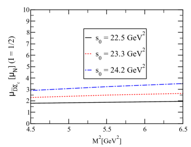
(a)

(b)

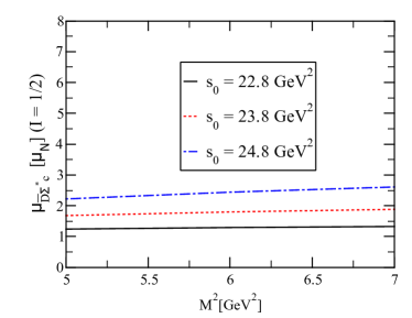
(c)

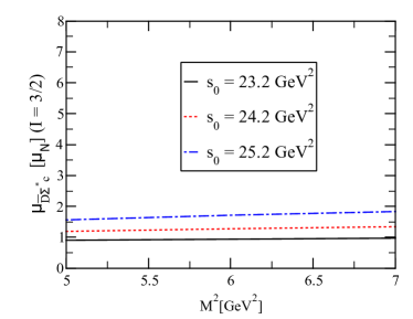
(d)

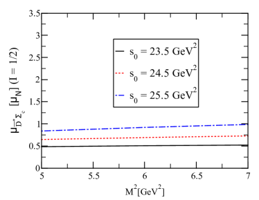
(e)

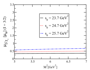
(f)

Figure 1: The magnetic moments of the isospin eigenstate $\bar{D}\Sigma_{c}$, $\bar{D}^{*}\Sigma_{c}$, and $\bar{D}\Sigma_{c}^{*}$ pentaquarks versus $\rm{M^{2}}$ at three different values of $\rm{s_{0}}$.

where $\Delta^{\mbox{DimN}}(\rm{M^{2}},\rm{s_{0}})=\Delta^{\mbox{Dim(10+11)}}(\rm{M^{2}},\rm{s_{0}})$. These constraints determine the working intervals of the auxiliary parameters $\rm{M^{2}}$ and $\rm{s_{0}}$. These intervals are presented in Table 1 for the states that have been studied. The values of PC and CVG obtained from the analyses for each state are also presented in this table. In Fig. 1 we also show the variation of the magnetic moments of the $\bar{D}\Sigma_{c}$, $\bar{D}^{*}\Sigma_{c}$, and $\bar{D}\Sigma_{c}^{*}$ pentaquarks, on $\rm{M^{2}}$ for different values of $\rm{s_{0}}$. As can be seen from the figure, the requirement for a mild variation of the results obtained in these regions is fulfilled as required. The residual dependencies appear as uncertainties in the results.

Table 1: Working intervals of $\rm{s_{0}}$ and $\rm{M^{2}}$ as well as the PC and CVG for the magnetic moments of isospin eigenstate $\bar{D}\Sigma_{c}$, $\bar{D}^{*}\Sigma_{c}$, and $\bar{D}\Sigma_{c}^{*}$ pentaquarks.

State	$J^{P}$	Isospin	$\rm{s_{0}}$ (GeV2)	$\rm{M^{2}}$ (GeV2)	PC ($\%$)	CVG ($\%$)
$\bar{D}\Sigma_{c}$	$\frac{1}{2}^{-}$	$\frac{1}{2}$	$22.4-24.2$	$4.5-6.5$	$32-58$	$1.82$
$\bar{D}\Sigma_{c}$	$\frac{1}{2}^{-}$	$\frac{3}{2}$	$22.4-24.2$	$4.5-6.5$	$31-58$	$1.80$
$\bar{D}\Sigma^{*}$	$\frac{3}{2}^{-}$	$\frac{1}{2}$	$22.8-24.8$	$5.0-7.0$	$31-55$	$1.90$
$\bar{D}\Sigma^{*}$	$\frac{3}{2}^{-}$	$\frac{3}{2}$	$23.2-25.2$	$5.0-7.0$	$30-55$	$1.80$
$\bar{D}^{*}\Sigma_{c}$	$\frac{3}{2}^{-}$	$\frac{1}{2}$	$23.5-25.5$	$5.0-7.0$	$31-54$	$1.92$
$\bar{D}^{*}\Sigma_{c}$	$\frac{3}{2}^{-}$	$\frac{3}{2}$	$23.5-25.5$	$5.0-7.0$	$30-53$	$1.90$

Once all the input parameters are determined, the final predictions for the magnetic moments of the isospin eigenstate $\bar{D}\Sigma_{c}$, $\bar{D}^{*}\Sigma_{c}$, and $\bar{D}\Sigma_{c}^{*}$ pentaquarks are given in Table 2. The errors shown in the numerical values are due to the uncertainties in the values of all input parameters, as well as the uncertainties resulting from the calculations of the working intervals for the helping parameters $\rm{M^{2}}$ and $\rm{s_{0}}$. We should mention here that the QCD sum rule calculations indicate that there is one $\bar{D}\Sigma^{*}$ molecular pentaquark candidate with a mass of about $4.38$ GeV with isospin-1/2, and it does not have to be the $\rm{P_{c}(4380)}$. We calculate the magnetic moment of this state, and since its mass is of the value mentioned, we chose this nomenclature.

Table 2: The magnetic moments of isospin eigenstate $\bar{D}\Sigma_{c}$, $\bar{D}^{*}\Sigma_{c}$, and $\bar{D}\Sigma_{c}^{*}$ pentaquarks. We have also introduced the electric quadrupole ($\mathcal{Q}$) and the magnetic octupole ($\mathcal{O}$) of the $\bar{D}^{*}\Sigma_{c}$, and $\bar{D}\Sigma_{c}^{*}$ pentaquarks.

State	$J^{P}$	Isospin	$\mu\,(\mu_{N})$	$\mathcal{Q}$ (fm2)($\times 10^{-2}$)	$\mathcal{O}$ (fm3)($\times 10^{-3}$)	Pentaquark
$\bar{D}\Sigma_{c}$	$\frac{1}{2}^{-}$	$\frac{1}{2}$	$2.59^{+0.92}_{-0.81}$	-	-	$\rm{P_{c}(4312)}$
$\bar{D}\Sigma_{c}$	$\frac{1}{2}^{-}$	$\frac{3}{2}$	$3.44^{+1.20}_{-1.06}$	-	-	-
$\bar{D}\Sigma^{*}$	$\frac{3}{2}^{-}$	$\frac{1}{2}$	$1.88^{+0.73}_{-0.64}$	$-1.92^{+0.62}_{-0.56}$	$-0.10^{+0.04}_{-0.03}$	$\rm{P_{c}(4380)}$
$\bar{D}\Sigma^{*}$	$\frac{3}{2}^{-}$	$\frac{3}{2}$	$1.34^{+0.50}_{-0.44}$	$-1.21^{+0.38}_{-0.34}$	$-0.06^{+0.03}_{-0.02}$	-
$\bar{D}^{*}\Sigma_{c}$	$\frac{3}{2}^{-}$	$\frac{1}{2}$	$0.73^{+0.26}_{-0.24}$	$-0.66^{+0.21}_{-0.20}$	$-0.037^{+0.013}_{-0.012}$	$\rm{P_{c}(4440)}$
$\bar{D}^{*}\Sigma_{c}$	$\frac{3}{2}^{-}$	$\frac{3}{2}$	$0.50^{+0.17}_{-0.16}$	$-0.43^{+0.12}_{-0.11}$	$-0.023^{+0.008}_{-0.007}$	-

The orders of the magnetic moments indicate that they are accessible in the experiment. Our calculations also show that the magnetic moments of $\bar{D}\Sigma_{c}$ states with isospin-1/2 and 3/2 are governed by the light quarks, while those of $\bar{D}^{*}\Sigma_{c}$, and $\bar{D}\Sigma_{c}^{*}$ states with isospin-1/2 and 3/2 are governed by the charm quark. A more detailed analysis shows that for the magnetic moment of the pentaquark $\rm{P_{c}(4312)}$, $75\%$ of the contribution comes from the $\bar{D}^{0}\Sigma_{c}^{+}$ component. For the pentaquark magnetic moment $\rm{P_{c}(4380)}$, $68\%$ of the contribution comes from the $\bar{D}^{0*}\Sigma_{c}^{+}$ component, while for the pentaquark $\rm{P_{c}(4440)}$, $60\%$ of the contribution comes from the $\bar{D}^{0}\Sigma_{c}^{+*}$ component. For the completeness of the analysis, the electric quadrupole and magnetic octupole moments of the spin-3/2 $\bar{D}^{*}\Sigma_{c}$ and $\bar{D}\Sigma_{c}^{*}$ pentaquark states are also obtained. It is well known that the sign of the electric quadrupole moment gives information about the shape of hadrons. Therefore, we can say that the shape of these pentaquarks is oblate.

In Ref. [21], the magnetic moments of the $\rm{P_{c}(4312)}$, $\rm{P_{c}(4380)}$, and $\rm{P_{c}(4440)}$ states are extracted within the quark model and the predicted results are $\mu_{\rm{P_{c}(4312)}}=1.76~{}\mu_{N}$, $\mu_{\rm{P_{c}(4380)}}=1.357~{}\mu_{N}$, and $\mu_{\rm{P_{c}(4440)}}=3.246~{}\mu_{N}$. In Ref. [24], the magnetic moment of the $\rm{P_{c}(4312)}$ pentaquark state was acquired through the QCD sum rule method in the external weak electromagnetic field by using a $\bar{D}^{-}\Sigma_{c}^{++}$ molecular configuration. The numerical value was obtained as $\mu_{\rm{P_{c}(4312)}}=1.75^{+0.15}_{-0.11}$ (we would like to point out that in this study it is not written whether the magnetic moment is in its natural unit or the nuclear magneton unit). In Refs. [25, 22, 27], the magnetic moments of the hidden-charm pentaquark states $\rm{P_{c}(4312)}$, $\rm{P_{c}(4380)}$, and $\rm{P_{c}(4440)}$ were obtained within the framework of the QCD light-cone sum rules by assuming them as $\bar{D}^{0}\Sigma_{c}^{+}$, $\bar{D}^{*-}\Sigma_{c}^{++}$, $\bar{D}^{*0}\Sigma_{c}^{+}$ molecular configurations with quantum numbers $\rm{J^{P}=\frac{1}{2}^{-}}$, $\rm{J^{P}=\frac{3}{2}^{-}}$, $\rm{J^{P}=\frac{3}{2}^{-}}$, respectively. The obtained results are presented as $\mu_{\rm{P_{c}(4312)}}=1.98\pm 0.75~{}\mu_{N}$, $\mu_{\rm{P_{c}(4380)}}=3.35\pm 1.35~{}\mu_{N}$, and $\mu_{\rm{P_{c}(4440)}}=3.49^{+1.49}_{-1.31}~{}\mu_{N}$. In Ref. [26], the magnetic moment of the $\rm{P_{c}(4312)}$ pentaquark state was extracted via quark model without/with coupled channel effects and the D-wave contributions, and the predicted result is given as $\mu_{\rm{P_{c}(4312)}}=1.624-1.737~{}\mu_{N}$. In Ref. [23], the magnetic moments of four hidden-charm pentaquark states are obtained with $\rm{J^{P}=\frac{3}{2}^{-}}$ in the quark model, and the obtained results are about $1.1-3.1~{}\rm{\mu_{N}}$. However, we should mention that all the masses of these four pentaquark states are lower than those of the observed hidden-charm pentaquark states. From these results, we observe that while the results obtained for the $\bar{D}\Sigma_{c}$ state are more or less similar, the results for the spin-3/2 pentaquark states $\bar{D}^{*}\Sigma_{c}$ and $\bar{D}\Sigma_{c}^{*}$ are different in magnitude and range.

IV summary

To shed light on the nature of the controversial and not yet fully understood exotic states, we are carrying out a systematic study of their electromagnetic properties. The magnetic moment of a hadron state is as fundamental a dynamical quantity as its mass and contains valuable information on the deep underlying structure. In this study, we use the QCD light-cone sum rule to extract the magnetic moments of the $\mathrm{P_{c}(4312)}$, $\mathrm{P_{c}(4380)}$, and $\mathrm{P_{c}(4440)}$ pentaquarks by considering them as the molecular picture with spin-parity $\mathrm{J^{P}=\frac{1}{2}^{-}}$, $\mathrm{J^{P}=\frac{3}{2}^{-}}$, and $\mathrm{J^{P}=\frac{3}{2}^{-}}$, respectively. We define the isospin of the interpolating currents of these states, which is the key to solving the puzzle of the hidden-charm pentaquark states, in order to make these analyses more precise and reliable. We compared our results with other theoretical predictions, which can be a useful complementary tool for interpreting the hidden-charm pentaquark sector and we observe that they are not in mutual agreement with each other. We have also calculated higher multipole moments for spin-3/2 $\bar{D}^{*}\Sigma_{c}$ and $\bar{D}\Sigma_{c}^{*}$ pentaquarks, indicating a non-spherical charge distribution.

We can obtain information about the internal structure of hadrons and about the behavior of the quarks that make them up by studying their magnetic moments. Understanding the structure and searching for it in the photo-production process would be aided by studying the magnetic moments of the pentaquarks, which could yield an independent probe of the hidden-charm pentaquarks. It will also be important to determine the branching ratios of the different decay modes and decay channels of the hidden-charm pentaquarks. Checking our predictions with future experiments could be very helpful in figuring out the geometric shape as well as the internal structure of these pentaquarks. We hope that this research, together with existing studies in the literature that include different properties of these pentaquark states, will encourage our colleagues to pay attention to the electromagnetic characteristics of pentaquark states in the future.

Appendix: Explicit expression for $\Delta_{1}^{\rm{QCD}}(\rm{M^{2}},\rm{s_{0}})$

In this appendix, we present the explicit expressions of the function $\Delta_{1}^{\rm{QCD}}(\rm{M^{2}},\rm{s_{0}})$ for the magnetic moment of the $\bar{D}\Sigma_{c}$ pentaquark state with isospin-1/2 entering into the sum rule.

$$\Delta_{1}^{\rm{QCD}}(\rm{M^{2}},\rm{s_{0}}) =\frac{m_{c}}{31708938240\pi^{7}}\Bigg{[}e_{c}\Bigg{(}-708I[0,7,1,3]+2478I[0,7,1,4]-3186I[0,7,1,5]+1770I[0,7,1,6]$$

$$-354I[0,7,1,7]+2128I[0,7,2,3]-5319I[0,7,2,4]+4254I[0,7,2,5]-1063I[0,7,2,6]$$

$$-2132I[0,7,3,3]+3196I[0,7,3,4]-1064I[0,7,3,5]+712I[0,7,4,3]-355I[0,7,4,4]$$

$$-2478I[1,6,1,4]+7434I[1,6,1,5]-7434I[1,6,1,6]+2478I[1,6,1,7]+7441I[1,6,2,4]$$

$$-14882I[1,6,2,5]+7441I[1,6,2,6]-7448I[1,6,3,4]+7448I[1,6,3,5]+2485I[1,6,4,4]\Bigg{)}$$

$$-6(11e_{d}+106e_{u})\Bigg{(}3I[0,7,2,2]-10I[0,7,2,3]+12I[0,7,2,4]-6I[0,7,2,5]+I[0,7,2,6]$$

$$-9I[0,7,3,2]+21I[0,7,3,3]-15I[0,7,3,4]+3I[0,7,3,5]+9I[0,7,4,2]-12I[0,7,4,3]$$

$$+3I[0,7,4,4]-3I[0,7,5,2]+I[0,7,5,3]+7I[1,6,2,3]-21I[1,6,2,4]+21I[1,6,2,5]$$

$$-7I[1,6,2,6]-21I[1,6,3,3]+42I[1,6,3,4]-21I[1,6,3,5]+21I[1,6,4,3]-21I[1,6,4,4]$$

$$-7I[1,6,5,3]\Bigg{)}\Bigg{]}$$

$$-\frac{m_{c}P_{1}P_{2}^{2}}{764411904\pi^{3}}\Bigg{[}3\Bigg{(}-8e_{d}I_{5}[\mathbb{A}]+e_{u}\Big{(}5I_{1}[\mathcal{S}]-4I_{1}[\mathcal{T}_{1}]+4I_{1}[\mathcal{T}_{2}]+I_{1}[\mathcal{T}_{3}]-I_{1}[\mathcal{T}_{4}]+5I_{2}[\mathcal{S}]+4I_{2}[\mathcal{T}_{1}]$$

$$-4I_{2}[\mathcal{T}_{2}]-I_{2}[\mathcal{T}_{3}]+I_{2}[\mathcal{T}_{4}]+6I_{5}[\mathbb{A}]\Big{)}\Bigg{)}I[0,2,3,0]-4\chi\Bigg{(}32e_{d}\Big{(}I[0,3,1,0]-2I[0,3,1,1]+I[0,3,1,2]$$

$$-2I[0,3,2,0]+2I[0,3,2,1]+I[0,3,3,0]\Big{)}+e_{u}\Big{(}17I[0,3,1,0]-39I[0,3,1,1]+27I[0,3,1,2]$$

$$-5I[0,3,1,3]-42I[0,3,2,0]+60I[0,3,2,1]-18I[0,3,2,2]+33I[0,3,3,0]-21I[0,3,3,1]$$

$$-8I[0,3,4,0]\Big{)}\Bigg{)}\varphi_{\gamma}[u_{0}]-6\chi m_{0}^{2}\Bigg{(}(4e_{d}-3e_{u})I_{5}[\varphi_{\gamma}]I[0,2,3,0]-2e_{u}\Big{(}I[0,2,1,0]-2I[0,2,1,1]$$

$$+I[0,2,1,2]-2I[0,2,2,0]+2I[0,2,2,1]+I[0,2,3,0]\Big{)}\varphi_{\gamma}[u_{0}]\Bigg{)}\Bigg{]}$$

$$-\frac{m_{c}^{2}P_{1}P_{2}}{24461180928\pi^{5}}\Bigg{[}-6e_{u}\Bigg{(}57I_{1}[\mathcal{S}]+18I_{1}[\mathcal{T}_{1}]+13I_{1}[\mathcal{T}_{2}]+12I_{1}[\mathcal{T}_{3}]-43I_{1}[\mathcal{T}_{4}]+I_{1}[\mathcal{\tilde{S}}]+57I2[\mathcal{S}]$$

$$-18I_{2}[\mathcal{T}_{1}]-13I_{2}[\mathcal{T}_{2}]-12I_{2}[\mathcal{T}_{3}]+43I_{2}[\mathcal{T}_{4}]+I_{2}[\mathcal{\tilde{S}}]-4\Big{(}45I_{3}[\mathcal{S}]-29I_{3}[\mathcal{T}_{1}]+29I_{3}[\mathcal{T}_{2}]-4I_{3}[\mathcal{T}_{]}$$

$$+4I_{3}[\mathcal{T}_{4}]+32I_{3}[\mathcal{\tilde{S}}]+45I4[\mathcal{S}]+29I_{4}[\mathcal{T}_{1}]-29I_{4}[\mathcal{T}_{2}]+4I_{4}[\mathcal{T}_{3}]-4I_{4}[\mathcal{T}_{4}]+32I_{4}[\mathcal{\tilde{S}}]\Big{)}\Bigg{)}I[0,3,2,0]$$

$$-3\Bigg{(}5(-10e_{d}+e_{u})I_{1}[\mathcal{S}]+2e_{d}\big{(}-25I_{1}[\mathcal{\tilde{S}}]+49I_{3}[\mathcal{S}]+I_{3}[\mathcal{\tilde{S}}]\big{)}+e_{u}\Big{(}-47I_{1}[\mathcal{T}_{1}]+23I_{1}[\mathcal{T}_{2}]-4I_{1}[\mathcal{T}_{3}]$$

$$+28I_{1}[\mathcal{T}_{4}]+10I_{1}[\mathcal{\tilde{S}}]+5I_{2}[\mathcal{S}]+47I_{2}[\mathcal{T}_{1}]-23I_{2}[\mathcal{T}_{2}]+2\big{(}2I_{2}[\mathcal{T}_{3}]-14I_{2}[\mathcal{T}_{4}]+5I_{2}[\mathcal{\tilde{S}}]+15I_{3}[\mathcal{S}]$$

$$+7I_{3}[\mathcal{T}_{1}]-7I_{3}[\mathcal{T}_{2}]-12I_{3}[\mathcal{T}_{3}]+12I_{3}[\mathcal{T}_{4}]+8I_{3}[\mathcal{\tilde{S}}]+15I_{4}[\mathcal{S}]-7I_{4}[\mathcal{T}_{1}]+7I_{4}[\mathcal{T}_{2}]+12I_{4}[\mathcal{T}_{3}]-12I_{4}[\mathcal{T}_{4}]$$

$$+8I_{4}[\mathcal{\tilde{S}}]\Big{)}\Big{)}\Bigg{)}I[0,3,3,0]+768f_{3\gamma}\pi^{2}\Bigg{(}3e_{u}m_{0}^{2}\Big{(}-I[0,1,1,0]+I[0,1,1,1]+I[0,1,2,0]\Big{)}$$

$$+6e_{d}\Big{(}5I[0,2,1,0]-8I[0,2,1,1]+3I[0,2,1,2]-8I[0,2,2,0]+6I[0,2,2,1]+3I[0,2,3,0]\Big{)}$$

$$+2e_{u}\Big{(}7I[0,2,1,0]-11I[0,2,1,1]+4I[0,2,1,2]-14I[0,2,2,0]+11I[0,2,2,1]+7I[0,2,3,0]\Big{)}\Bigg{)}\psi^{a}[u_{0}]$$

$$+4\chi\Bigg{(}6e_{d}\Big{(}40I[0,4,1,1]-88I[0,4,1,2]+48I[0,4,1,3]-3I[0,4,2,0]-74I[0,4,2,1]+85I[0,4,2,2]+6I[0,4,3,0]$$

$$+34I[0,4,3,1]-3I[0,4,4,0]\Big{)}+e_{u}\Big{(}216I[0,4,1,1]-438I[0,4,1,2]+260I[0,4,1,3]-38I[0,4,1,4]+6I[0,4,2,0]$$

$$-441I[0,4,2,1]+492I[0,4,2,2]-89I[0,4,2,3]-12I[0,4,3,0]+222I[0,4,3,1]-48I[0,4,3,2]+6I[0,4,4,0]$$

$$+3I[0,4,4,1]\Big{)}\Bigg{)}\varphi_{\gamma}[u_{0}]\Bigg{]}$$

$$+\frac{P_{1}f_{3\gamma}m_{c}^{2}}{130459631616\pi^{5}}\Bigg{[}3e_{u}\Big{(}62I[0,4,3,0]-7I[0,4,4,0]\Big{)}I_{2}[\mathcal{A}]+\Big{(}192e_{d}I[0,4,3,0]+54e_{u}I[0,4,3,0]+624e_{d}I[0,4,4,0]$$

$$+577e_{u}I[0,4,4,0]\Big{)}I_{2}[\mathcal{V}]+\Big{(}128e_{d}I[0,4,3,0]+1398e_{u}I[0,4,3,0]-146e_{d}I[0,4,4,0]+4945e_{u}I[0,4,4,0]\Big{)}I_{1}[\mathcal{V}]$$

$$+64\Big{(}(3e_{d}-e_{u})I_{5}[\psi^{a}]+8e_{u}I_{6}[\psi_{\gamma}^{\nu}]\Big{)}I[0,4,3,0]-32\Big{(}(390e_{d}-1097e_{u})I_{5}[\psi^{a}]+16e_{u}I_{6}[\psi_{\gamma}^{\nu}]\Big{)}I[0,4,4,0]$$

$$-16\Bigg{(}24e_{d}\Big{(}21I[0,4,1,0]-79I[0,4,1,1]+113I[0,4,1,2]-73I[0,4,1,3]+18I[0,4,1,4]-77I[0,4,2,0]$$

$$+216I[0,4,2,1]-205I[0,4,2,2]+66I[0,4,2,3]+91I[0,4,3,0]-167I[0,4,3,1]+78I[0,4,3,2]-35I[0,4,4,0]$$

$$+30I[0,4,4,1]\Big{)}+e_{u}\Big{(}-3024I[0,4,1,0]+8688I[0,4,1,1]-7912I[0,4,1,2]+1856I[0,4,1,3]+392I[0,4,1,4]$$

$$+11091I[0,4,2,0]-20765I[0,4,2,1]+8241I[0,4,2,2]+1433I[0,4,2,3]-13113I[0,4,3,0]+11434I[0,4,3,1]$$

$$+1687I[0,4,3,2]+5049I[0,4,4,0]+643I[0,4,4,1]-3I[0,4,5,0]\Big{)}\Bigg{)}\psi^{a}[u_{0}]\Bigg{]}$$

$$+\frac{m_{c}^{2}P_{2}}{6794772480\pi^{5}}\Bigg{[}-12\Bigg{(}2(e_{d}-2e_{u})I_{1}[\mathcal{S}]+euI_{1}[\mathcal{T}_{1}]+2e_{d}\big{(}I_{1}[\mathcal{\tilde{S}}]-3I3[\mathcal{S}]-3I3[\mathcal{\tilde{S}}]\big{)}-e_{u}\Big{(}2I_{1}[\mathcal{T}_{2}]-I_{1}[\mathcal{T}_{3}]+2I_{1}[\mathcal{\tilde{S}}]$$

$$+4I_{2}[\mathcal{S}]+I_{2}[\mathcal{T}_{1}]-2I_{2}[\mathcal{T}_{2}]+I_{2}[\mathcal{T}_{3}]+2I_{2}[\mathcal{\tilde{S}}]-6\big{(}3I_{3}[\mathcal{S}]-2I_{3}[\mathcal{T}_{1}]+2I_{3}[\mathcal{T}_{2}]-I_{3}[\mathcal{T}_{3}]+I_{3}[\mathcal{T}_{4}]+2I_{3}[\mathcal{\tilde{S}}]+3I_{4}[\mathcal{S}]$$

$$+2I_{4}[\mathcal{T}_{1}]-2I_{4}[\mathcal{T}_{2}]+I_{4}[\mathcal{T}_{3}]-I_{4}[\mathcal{T}_{4}]+2I_{4}[\mathcal{\tilde{S}}]\big{)}\Big{)}\Bigg{)}I[0,5,3,0]-1920f_{3\gamma}\pi^{2}\Bigg{(}e_{d}\Big{(}6m_{0}^{2}\big{(}I[0,3,2,0]-2I[0,3,2,1]$$

$$+I[0,3,2,2]-2I[0,3,3,0]+2I[0,3,3,1]+I[0,3,4,0]\big{)}+7I[0,4,2,0]-20I[0,4,2,1]+19I[0,4,2,2]-6I[0,4,2,3]$$

$$-14I[0,4,3,0]+26I[0,4,3,1]-12I[0,4,3,2]+7I[0,4,4,0]-6I[0,4,4,1]\Big{)}+e_{u}\Big{(}5m_{0}^{2}\big{(}I[0,3,2,0]-2I[0,3,2,1]$$

$$+I[0,3,2,2]-2I[0,3,3,0]+2I[0,3,3,1]+I[0,3,4,0]\big{)}-42I[0,4,2,0]+79I[0,4,2,1]-32I[0,4,2,2]-5I[0,4,2,3]$$

$$+84I[0,4,3,0]-74I[0,4,3,1]-10I[0,4,3,2]-42I[0,4,4,0]-5I[0,4,4,1]\Big{)}\Bigg{)}\psi^{a}[u_{0}]\Bigg{]}$$

$$+\frac{m_{c}\,f_{3\gamma}}{27179089920\pi^{5}}\Bigg{[}4\Big{(}-3e_{d}I_{1}[\mathcal{V}]+5e_{u}\big{(}I_{1}[\mathcal{A}]+I_{1}[\mathcal{V}]-I_{2}[\mathcal{A}]+I_{2}[\mathcal{V}]\big{)}\Big{)}I[0,6,4,0]-9\Big{(}-4e_{d}\big{(}I_{1}[\mathcal{V}]-6I_{2}[\mathcal{V}]\big{)}$$

$$+e_{u}\big{(}3I_{1}[\mathcal{A}]+193I_{1}[\mathcal{V}]-3I_{2}[\mathcal{A}]+25I_{2}[\mathcal{V}]\big{)}\Big{)}I[0,6,5,0]+72\Bigg{(}2e_{d}\Big{(}13I[0,6,2,1]-45I[0,6,2,2]+57I[0,6,2,3]$$

$$-31I[0,6,2,4]+6I[0,6,2,5]-39I[0,6,3,1]+96I[0,6,3,2]-75I[0,6,3,3]+18I[0,6,3,4]+39I[0,6,4,1]$$

$$-57I[0,6,4,2]+18I[0,6,4,3]-13I[0,6,5,1]+6I[0,6,5,2]\Big{)}+e_{u}\Big{(}-168I[0,6,2,1]+493I[0,6,2,2]-471I[0,6,2,3]$$

$$+135I[0,6,2,4]+11I[0,6,2,5]+504I[0,6,3,1]-975I[0,6,3,2]+438I[0,6,3,3]+33I[0,6,3,4]-504I[0,6,4,1]$$

$$+471I[0,6,4,2]+33I[0,6,4,3]+168I[0,6,5,1]+11I[0,6,5,2]\Big{)}\Bigg{)}\psi^{a}[u_{0}]\Bigg{]},$$ (33)

where $P_{1}=\langle g_{s}^{2}G^{2}\rangle$ is gluon condensate, and $P_{2}=\langle\bar{q}q\rangle$ stands for u/d-quark condensate. The functions $I[n,m,l,k]$ and $I_{i}[\mathcal{F}]$ are written as follows:

$$I[n,m,l,k] =\int_{4m_{c}^{2}}^{\rm{s_{0}}}ds\int_{0}^{1}dt\int_{0}^{1}dw~{}e^{-s/\rm{M^{2}}}~{}s^{n}\,(s-4\,m_{c}^{2})^{m}\,t^{l}\,w^{k},$$

$$I_{1}[\mathcal{F}] =\int D_{\alpha_{i}}\int_{0}^{1}dv~{}\mathcal{F}(\alpha_{\bar{q}},\alpha_{q},\alpha_{g})\delta^{\prime}(\alpha_{q}+\bar{v}\alpha_{g}-u_{0}),$$

$$I_{2}[\mathcal{F}] =\int D_{\alpha_{i}}\int_{0}^{1}dv~{}\mathcal{F}(\alpha_{\bar{q}},\alpha_{q},\alpha_{g})\delta^{\prime}(\alpha_{\bar{q}}+v\alpha_{g}-u_{0}),$$

$$I_{3}[\mathcal{F}] =\int D_{\alpha_{i}}\int_{0}^{1}dv~{}\mathcal{F}(\alpha_{\bar{q}},\alpha_{q},\alpha_{g})\delta(\alpha_{q}+\bar{v}\alpha_{g}-u_{0}),$$

$$I_{4}[\mathcal{F}] =\int D_{\alpha_{i}}\int_{0}^{1}dv~{}\mathcal{F}(\alpha_{\bar{q}},\alpha_{q},\alpha_{g})\delta(\alpha_{\bar{q}}+v\alpha_{g}-u_{0}),$$

$$I_{5}[\mathcal{F}] =\int_{0}^{1}du~{}\mathcal{F}(u)\delta^{\prime}(u-u_{0}),$$

$$I_{6}[\mathcal{F}] =\int_{0}^{1}du~{}\mathcal{F}(u),$$ (34)

where $\mathcal{F}$ stands for the associated photon distribution amplitudes.

References

- [1] R. Aaij, et al., Observation of Resonances Consistent with Pentaquark States in Decays, Phys. Rev. Lett. 115 (2015) 072001. arXiv:1507.03414, doi:10.1103/PhysRevLett.115.072001.
- [2] R. Aaij, et al., Observation of a narrow pentaquark state, , and of two-peak structure of the , Phys. Rev. Lett. 122 (22) (2019) 222001. arXiv:1904.03947, doi:10.1103/PhysRevLett.122.222001.
- [3] R. Aaij, et al., Evidence for a new structure in the and systems in decays, Phys. Rev. Lett. 128 (6) (2022) 062001. arXiv:2108.04720, doi:10.1103/PhysRevLett.128.062001.
- [4] Observation of a resonance consistent with a strange pentaquark candidate in decays (10 2022). arXiv:2210.10346.
- [5] A. Esposito, A. L. Guerrieri, F. Piccinini, A. Pilloni, A. D. Polosa, Four-Quark Hadrons: an Updated Review, Int. J. Mod. Phys. A 30 (2015) 1530002. arXiv:1411.5997, doi:10.1142/S0217751X15300021.
- [6] A. Esposito, A. Pilloni, A. D. Polosa, Multiquark Resonances, Phys. Rept. 668 (2017) 1–97. arXiv:1611.07920, doi:10.1016/j.physrep.2016.11.002.
- [7] S. L. Olsen, T. Skwarnicki, D. Zieminska, Nonstandard heavy mesons and baryons: Experimental evidence, Rev. Mod. Phys. 90 (1) (2018) 015003. arXiv:1708.04012, doi:10.1103/RevModPhys.90.015003.
- [8] R. F. Lebed, R. E. Mitchell, E. S. Swanson, Heavy-Quark QCD Exotica, Prog. Part. Nucl. Phys. 93 (2017) 143–194. arXiv:1610.04528, doi:10.1016/j.ppnp.2016.11.003.
- [9] M. Nielsen, F. S. Navarra, S. H. Lee, New Charmonium States in QCD Sum Rules: A Concise Review, Phys. Rept. 497 (2010) 41–83. arXiv:0911.1958, doi:10.1016/j.physrep.2010.07.005.
- [10] N. Brambilla, S. Eidelman, C. Hanhart, A. Nefediev, C.-P. Shen, C. E. Thomas, A. Vairo, C.-Z. Yuan, The states: experimental and theoretical status and perspectives, Phys. Rept. 873 (2020) 1–154. arXiv:1907.07583, doi:10.1016/j.physrep.2020.05.001.
- [11] S. Agaev, K. Azizi, H. Sundu, Four-quark exotic mesons, Turk. J. Phys. 44 (2) (2020) 95–173. arXiv:2004.12079, doi:10.3906/fiz-2003-15.
- [12] H.-X. Chen, W. Chen, X. Liu, S.-L. Zhu, The hidden-charm pentaquark and tetraquark states, Phys. Rept. 639 (2016) 1–121. arXiv:1601.02092, doi:10.1016/j.physrep.2016.05.004.
- [13] A. Ali, J. S. Lange, S. Stone, Exotics: Heavy Pentaquarks and Tetraquarks, Prog. Part. Nucl. Phys. 97 (2017) 123–198. arXiv:1706.00610, doi:10.1016/j.ppnp.2017.08.003.
- [14] F.-K. Guo, C. Hanhart, U.-G. Meißner, Q. Wang, Q. Zhao, B.-S. Zou, Hadronic molecules, Rev. Mod. Phys. 90 (1) (2018) 015004, [Erratum: Rev.Mod.Phys. 94, 029901 (2022)]. arXiv:1705.00141, doi:10.1103/RevModPhys.90.015004.
- [15] Y.-R. Liu, H.-X. Chen, W. Chen, X. Liu, S.-L. Zhu, Pentaquark and Tetraquark states, Prog. Part. Nucl. Phys. 107 (2019) 237–320. arXiv:1903.11976, doi:10.1016/j.ppnp.2019.04.003.
- [16] G. Yang, J. Ping, J. Segovia, Tetra- and penta-quark structures in the constituent quark model, Symmetry 12 (11) (2020) 1869. arXiv:2009.00238, doi:10.3390/sym12111869.
- [17] X.-K. Dong, F.-K. Guo, B.-S. Zou, A survey of heavy-antiheavy hadronic molecules, Progr. Phys. 41 (2021) 65–93. arXiv:2101.01021, doi:10.13725/j.cnki.pip.2021.02.001.
- [18] X.-K. Dong, F.-K. Guo, B.-S. Zou, A survey of heavy–heavy hadronic molecules, Commun. Theor. Phys. 73 (12) (2021) 125201. arXiv:2108.02673, doi:10.1088/1572-9494/ac27a2.
- [19] L. Meng, B. Wang, G.-J. Wang, S.-L. Zhu, Chiral perturbation theory for heavy hadrons and chiral effective field theory for heavy hadronic molecules (4 2022). arXiv:2204.08716.
- [20] H.-X. Chen, W. Chen, X. Liu, Y.-R. Liu, S.-L. Zhu, An updated review of the new hadron states, Rept. Prog. Phys. 86 (2) (2023) 026201. arXiv:2204.02649, doi:10.1088/1361-6633/aca3b6.
- [21] G.-J. Wang, R. Chen, L. Ma, X. Liu, S.-L. Zhu, Magnetic moments of the hidden-charm pentaquark states, Phys. Rev. D 94 (9) (2016) 094018. arXiv:1605.01337, doi:10.1103/PhysRevD.94.094018.
- [22] U. Özdem, K. Azizi, Electromagnetic multipole moments of the pentaquark in light-cone QCD, Eur. Phys. J. C 78 (5) (2018) 379. arXiv:1803.06831, doi:10.1140/epjc/s10052-018-5873-2.
- [23] E. Ortiz-Pacheco, R. Bijker, C. Fernández-Ramírez, Hidden charm pentaquarks: mass spectrum, magnetic moments, and photocouplings, J. Phys. G 46 (6) (2019) 065104. arXiv:1808.10512, doi:10.1088/1361-6471/ab096d.
- [24] Y.-J. Xu, Y.-L. Liu, M.-Q. Huang, The magnetic moment of as a molecular state, Eur. Phys. J. C 81 (5) (2021) 421. arXiv:2008.07937, doi:10.1140/epjc/s10052-021-09211-8.
- [25] U. Özdem, Electromagnetic properties of the (4312) pentaquark state, Chin. Phys. C 45 (2) (2021) 023119. doi:10.1088/1674-1137/abd01c.
- [26] M.-W. Li, Z.-W. Liu, Z.-F. Sun, R. Chen, Magnetic moments and transition magnetic moments of Pc and Pcs states, Phys. Rev. D 104 (5) (2021) 054016. arXiv:2106.15053, doi:10.1103/PhysRevD.104.054016.
- [27] U. Özdem, Magnetic dipole moments of the hidden-charm pentaquark states: , and , Eur. Phys. J. C 81 (4) (2021) 277. arXiv:2102.01996, doi:10.1140/epjc/s10052-021-09070-3.
- [28] F. Gao, H.-S. Li, Magnetic moments of hidden-charm strange pentaquark states*, Chin. Phys. C 46 (12) (2022) 123111. arXiv:2112.01823, doi:10.1088/1674-1137/ac8651.
- [29] U. Özdem, Magnetic moments of pentaquark states in light-cone sum rules, Eur. Phys. J. A 58 (3) (2022) 46. doi:10.1140/epja/s10050-022-00700-2.
- [30] U. Özdem, Electromagnetic properties of doubly heavy pentaquark states, Eur. Phys. J. Plus 137 (2022) 936. arXiv:2201.00979, doi:10.1140/epjp/s13360-022-03125-4.
- [31] U. Özdem, Investigation of magnetic moment of Pcs(4338) and Pcs(4459) pentaquark states, Phys. Lett. B 836 (2023) 137635. arXiv:2208.07684, doi:10.1016/j.physletb.2022.137635.
- [32] F.-L. Wang, H.-Y. Zhou, Z.-W. Liu, X. Liu, What can we learn from the electromagnetic properties of hidden-charm molecular pentaquarks with single strangeness?, Phys. Rev. D 106 (5) (2022) 054020. arXiv:2208.10756, doi:10.1103/PhysRevD.106.054020.
- [33] U. Özdem, Electromagnetic properties of D¯(*)c’, D¯(*)c, D¯s(*)c and D¯s(*)c pentaquarks, Phys. Lett. B 846 (2023) 138267. arXiv:2303.10649, doi:10.1016/j.physletb.2023.138267.
- [34] F.-L. Wang, X. Liu, Higher molecular Ps/ pentaquarks arising from the c(’,*)D¯1/c(’,*)D¯2* interactions, Phys. Rev. D 108 (5) (2023) 054028. arXiv:2307.08276, doi:10.1103/PhysRevD.108.054028.
- [35] F.-L. Wang, X. Liu, Surveying the mass spectra and the electromagnetic properties of the molecular pentaquarks (11 2023). arXiv:2311.13968.
- [36] F. Guo, H.-S. Li, Analysis of the hidden-charm pentaquark states based on magnetic moment and transition magnetic moment (4 2023). arXiv:2304.10981.
- [37] V. L. Chernyak, I. R. Zhitnitsky, B meson exclusive decays into baryons, Nucl. Phys. B 345 (1990) 137–172. doi:10.1016/0550-3213(90)90612-H.
- [38] V. M. Braun, I. E. Filyanov, QCD Sum Rules in Exclusive Kinematics and Pion Wave Function, Z. Phys. C 44 (1989) 157. doi:10.1007/BF01548594.
- [39] I. I. Balitsky, V. M. Braun, A. V. Kolesnichenko, Radiative Decay Sigma+ — p gamma in Quantum Chromodynamics, Nucl. Phys. B 312 (1989) 509–550. doi:10.1016/0550-3213(89)90570-1.
- [40] K.-C. Yang, W. Y. P. Hwang, E. M. Henley, L. S. Kisslinger, QCD sum rules and neutron proton mass difference, Phys. Rev. D 47 (1993) 3001–3012. doi:10.1103/PhysRevD.47.3001.
- [41] V. M. Belyaev, B. Y. Blok, CHARMED BARYONS IN QUANTUM CHROMODYNAMICS, Z. Phys. C 30 (1986) 151. doi:10.1007/BF01560689.
- [42] P. Ball, V. M. Braun, N. Kivel, Photon distribution amplitudes in QCD, Nucl. Phys. B 649 (2003) 263–296. arXiv:hep-ph/0207307, doi:10.1016/S0550-3213(02)01017-9.
- [43] R. L. Workman, et al., Review of Particle Physics, PTEP 2022 (2022) 083C01. doi:10.1093/ptep/ptac097.
- [44] B. L. Ioffe, QCD at low energies, Prog. Part. Nucl. Phys. 56 (2006) 232–277. arXiv:hep-ph/0502148, doi:10.1016/j.ppnp.2005.05.001.
- [45] R. D. Matheus, S. Narison, M. Nielsen, J. M. Richard, Can the X(3872) be a 1++ four-quark state?, Phys. Rev. D 75 (2007) 014005. arXiv:hep-ph/0608297, doi:10.1103/PhysRevD.75.014005.
- [46] J. Rohrwild, Determination of the magnetic susceptibility of the quark condensate using radiative heavy meson decays, JHEP 09 (2007) 073. arXiv:0708.1405, doi:10.1088/1126-6708/2007/09/073.
- [47] X.-W. Wang, Z.-G. Wang, G.-L. Yu, Q. Xin, Isospin eigenstates of the color singlet-singlet-type pentaquark states, Sci. China Phys. Mech. Astron. 65 (8) (2022) 291011. arXiv:2201.06710, doi:10.1007/s11433-022-1915-2.