ClipSAM: CLIP and SAM Collaboration for Zero-Shot Anomaly Segmentation

Abstract

Recently, foundational models such as CLIP and SAM have shown promising performance for the task of Zero-Shot Anomaly Segmentation (ZSAS). However, either CLIP-based or SAM-based ZSAS methods still suffer from non-negligible key drawbacks: 1) CLIP primarily focuses on global feature alignment across different inputs, leading to imprecise segmentation of local anomalous parts; 2) SAM tends to generate numerous redundant masks without proper prompt constraints, resulting in complex post-processing requirements. In this work, we innovatively propose a CLIP and SAM collaboration framework called ClipSAM for ZSAS. The insight behind ClipSAM is to employ CLIP’s semantic understanding capability for anomaly localization and rough segmentation, which is further used as the prompt constraints for SAM to refine the anomaly segmentation results. In details, we introduce a crucial Unified Multi-scale Cross-modal Interaction (UMCI) module for interacting language with visual features at multiple scales of CLIP to reason anomaly positions. Then, we design a novel Multi-level Mask Refinement (MMR) module, which utilizes the positional information as multi-level prompts for SAM to acquire hierarchical levels of masks and merges them. Extensive experiments validate the effectiveness of our approach, achieving the optimal segmentation performance on the MVTec-AD and VisA datasets. Our code is public.

1 Introduction

Zero-Shot Anomaly Segmentation (ZSAS) is a critical task in fields such as image analysis Fomalont (1999) and industrial quality inspection Mishra et al. (2021); Bergmann et al. (2022, 2019). Its objective is to accurately localize and segment anomalous regions within images, without relying on prior class-specific training samples. As a result, the diversity of industrial products and the uncertainty in anomaly types pose significant challenges for the ZSAS task.

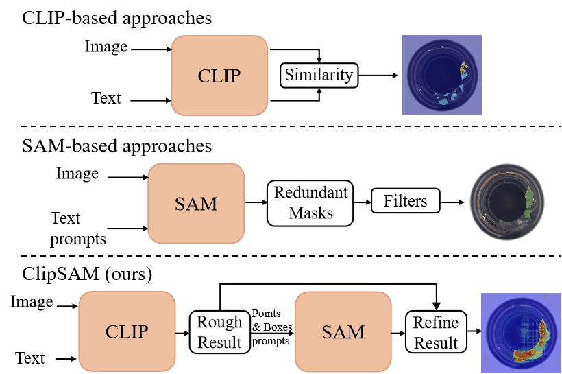
Figure 1: Structural comparisons among different approaches for Zero-Shot Anomaly Segmentation. Top: CLIP-based approaches. Middle: SAM-based approaches. Bottom: Our ClipSAM approach that leverages the strengths of both CLIP and SAM methods.

With the emergence of foundational models such as CLIP Radford et al. (2021) and SAM Kirillov et al. (2023), the notable advancements have been achieved in Zero-Shot Anomaly Segmentation. As depicted in Figure 1, the CLIP-based approaches, like WinCLIP Jeong et al. (2023) and APRIL-GAN Chen et al. (2023a), determine the anomaly classification of each patch by comparing the similarity between image patch tokens and text tokens. While CLIP exhibits a strong semantic understanding capability, it is achieved by aligning the global features of language and vision, making it less suitable for fine-grained segmentation tasks Wang et al. (2022). Due to the fact that anomalies consistently manifest in specific regions of objects, the global semantic consistency inherent in CLIP is unable to achieve precise identification of the edges of local anomalies. On the other hand, researchers have explored the SAM-based approaches to assist the ZSAS task. SAM has superior segmentation capabilities and can accept diverse prompts, including points, boxes, and textual prompts, to guide the segmentation process. To this end, SAA Cao et al. (2023), as shown in Figure 1, utilizes the SAM with textual prompts to generate vast candidate masks and applies filters for post-processing. However, simple textual prompts may be insufficient for accurately describing anomalous regions, resulting in subpar anomaly localization performance and underutilization of SAM’s capabilities. Meanwhile, the ambiguous prompts lead to the generation of redundant masks, which requires further selection of correct masks.

Based on these observations, we innovatively propose a CLIP and SAM collaboration framework, first employing CLIP for anomaly localization and rough segmentation and then utilizing SAM and the localization information to refine the anomaly segmentation results. For the stage of CLIP, it is crucial to incorporate the fusion of language tokens and image patch tokens and model their dependencies to strengthen CLIP’s ability to segment anomaly parts, since cross-modal interaction and fusion have been proven to be beneficial for localization and object segmentation in several studies Jing et al. (2021); Xu et al. (2023); Feng et al. (2021). Further, several notable works Ding et al. (2019); Huang et al. (2019); Hou et al. (2020) have focused on enhancing the model’s local semantic comprehension by paying attention to row and column features. Motivated by these studies, we have developed a novel cross-modal interaction strategy that facilitates the interaction of text and visual features at both row-column and multi-scale levels, adequately enhancing CLIP’s capabilities for positioning and segmenting anomaly parts. For the stage of SAM, in order to fully harness its fine-grained segmentation capability, we exploit the localization abilities of CLIP to provide more explicit prompts in the form of both points and bounding boxes. This approach greatly enhances SAM’s ability to segment anomaly regions accurately. Further, we have noticed that SAM’s segmentation results often display masks with different levels of granularity, even when provided with the same prompt. To avoid the inefficient post-processing caused by further mask filtering, we propose a more efficient mask refinement strategy that seamlessly integrates different levels of masks, leading to enhanced anomaly segmentation results.

As a conclusion, we propose a novel two-stage framework named CLIP and SAM Collaboration (ClipSAM) for ZSAS. The structural comparisons with previous works are illustrated in Figure 1. In the first stage, we employ CLIP for localization and rough segmentation. To achieve the fusion of multi-modal features at different levels, we design the Unified Multi-scale Cross-modal Interaction (UMCI) module. UMCI aggregates image patch tokens from both horizontal and vertical directions and utilizes the corresponding row and column features to interact with language features to perceive local anomalies in different directions. UMCI also considers the interaction of language and multi-scale visual features. In the second stage, we exploit the CLIP’s localization information to guide SAM for segmentation refinement. Specifically, we propose the Multi-level Mask Refinement (MMR) module, which first extracts diverse point and bounding box prompts from the CLIP’s anomaly localization results and then uses these prompts to guide SAM to generate precise masks. Finally, we fuse these masks with the results obtained from CLIP based on different mask confidences. Our main contributions can be summarized as follows:

• We propose a novel framework named CLIP and SAM Collaboration (ClipSAM) to fully leverage the characteristics of different large models for ZSAS. Specifically, we first use CLIP to locate and roughly segment the anomaly objects, and then refine the segmentation results with SAM and the positioning information.

• To better assist CLIP in realizing desired localization and rough segmentation, we propose the Unified Multi-scale Cross-modal Interaction (UMCI) module, which learns local and global semantics about anomalous parts by interacting language features with visual features at both row-column and multi-scale levels.

• To refine the segmentation results with SAM adequately, we designed the Multi-level Mask Refinement (MMR) module. It extracts point and bounding box prompts from the CLIP’s localization information to guide SAM in generating accurate masks, and fuse them with the results of CLIP to achieve fine-grained segmentation.

• Extensive experiments on various datasets consistently validate that our approach can achieve new state-of-the-art zero-shot anomaly segmentation results. Particularly on the MVTec-AD dataset, our method outperforms the SAM-based method by +19.1↑ in pixel-level AUROC, +10.0↑ in $F_{1}$-max and +45.5↑ in Pro metrics.

2 Related Work

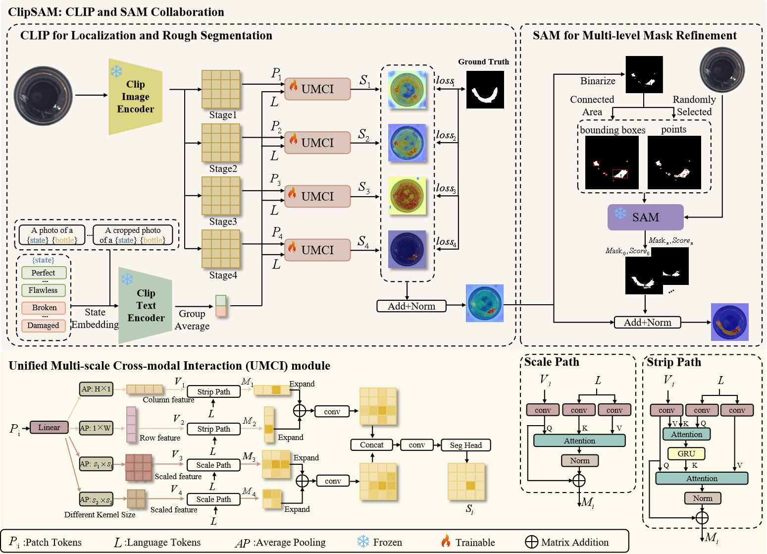
Figure 2: Overview of the proposed ClipSAM framework. ClipSAM includes two main processes: using CLIP for localization and rough segmentation, and using positioning information to prompt SAM to refine the segmentation results. These processes contain two important components: the Unified Multi-scale Cross-modal Interaction (UMCI) module and the Multi-level Mask Refinement (MMR) module. The UMCI module is employed for the interaction of language features with visual features of different directions and scales, facilitating CLIP’s ability to locate and segment anomaly objects. Meanwhile, the MMR module combines SAM, and uses point and box prompts extracted from location information to guide SAM to output the desired masks, and fuses them with the rough segmentation result obtained by CLIP.

2.1 Zero-shot Anomaly Segmentation

The methods for Zero-Shot Anomaly Segmentation (ZSAS) can be mainly divided into two categories. The first category is based on CLIP. As the pioneering work, WinCLIP Jeong et al. (2023) calculates the similarity between image patch tokens and textual features for ZSAS. Further, APRIL-GAN Chen et al. (2023a) employs linear layers to better align features of different modalities. AnoVL Deng et al. (2023) and ANOMALYCLIP Zhou et al. (2023) propose to enhance the generalization of text. SDP Chen et al. (2023b) proposes to address noise in the encoding process of the CLIP image encoder. The second category is based on SAM. Specifically, SAA Cao et al. (2023) utilizes text prompts for SAM to generate vast candidate masks and uses a complex evaluation mechanism to filter out irrelevant masks.

However, relying solely on CLIP or SAM may lead to certain limitations. For instance, CLIP-based methods struggle with precise segmentation of local anomalies, while SAM-based methods heavily rely on specific prompts. To address these drawbacks, we explore the collaboration mechanism of CLIP and SAM and propose a novel framework to leverage their strengths. Besides, we further design the Unified Multi-scale Cross-modal Interaction (UMCI) module and Multi-level Mask Refinement module to better exploit the specific ability of CLIP and SAM, respectively.

2.2 Foundation Models

Recently, there has been an increasing focus and attention on foundation models. Various foundation models have achieved satisfactory performance on kinds of downstream tasks Devlin et al. (2018); Brown et al. (2020). Notably, CLIP Radford et al. (2021) and SAM Kirillov et al. (2023) have emerged as two representative models with impressive zero-shot reasoning capabilities in classification and segmentation tasks, respectively. More specifically, CLIP focuses on aligning multi-modal features and possesses robust semantic understanding abilities for both language and vision, while SAM excels in achieving fine-grained segmentation based on different prompts. Recently, Yue et al. (2023) attempts to establish a connection between SAM’s image encoder and CLIP’s text encoder for surgical instrument segmentation, Wang et al. (2023) attempts to merge SAM and CLIP to facilitate downstream tasks. These works highlight the critical importance of exploring collaboration among foundational models.

2.3 Cross-modal Interaction

In the field of multi-modal learning, cross-modal interaction is becoming increasingly important. Specifically, Hu et al. (2016) concatenates features from different modalities and uses convolutions for multi-modal information fusion. Further, STEP Chen et al. (2019) establishes correlations between important areas in the image and relevant keywords in the text to enhance the fusion of cross-modal information. BRINet Feng et al. (2021) exchanges cross-modal information between different blocks of the encoder to facilitate image segmentation. The success of cross-modal interaction in diverse domains has motivated us to explore it in the context of zero-shot anomaly segmentation. To effectively address the challenge of localizing abnormal regions within an object, we introduce the Unified Multi-scale Cross-modal Interaction module, taking into account the interaction between text and both row-column and multi-scaled visual features.

3 Methodology

3.1 CLIP and SAM Collaboration

CLIP has a strong semantic understanding of different modalities, while SAM can easily detect edges of fine-grained objects, both of which are important for anomaly segmentation. In this paper, we present a novel CLIP and SAM collaboration framework called ClipSAM, which aims to boost the performance of ZSAS. The overview architecture is illustrated in Fig. 2. Specifically, we leverage the CLIP for initial rough segmentation and utilize it as a constraint to refine the segmentation results with SAM. In Sec. 3.2, we introduce the Unified Multi-scale Cross-modal Interaction (UMCI) module within the CLIP stage to achieve accurate rough segmentation and anomaly localization. In Sec. 3.3, we design the Multi-level Mask Refinement (MMR) module, which incorporates the guidance from CLIP to facilitate SAM in generating more precise masks for achieving fine-grained segmentation. In addition, the optimization function of the overall framework is discussed in Sec. 3.4.

3.2 Unified Multi-scale Cross-modal Interaction

In our ClipSAM framework, the CLIP encoder is employed to process both text and image inputs. For a specific pair of text and image, the encoder generates two outputs: $L\in\mathbb{R}^{C_{t}\times 2}$ and $P_{i}\in\mathbb{R}^{H\times W\times C}$. Here, $L$ represents the textual feature vector, in line with WinCLIP Jeong et al. (2023), reflecting two categories of normal and abnormal. $P_{i}$ denotes the patch tokens derived from the i-th stage of the encoder. For more details of the textual feature $L$, please refer to Appendix A.

As discussed in Sec. 1, cross-modal fusion has been proven to be beneficial for object segmentation. To achieve this, the Unified Multi-scale Cross-modal Interaction (UMCI) module is designed. Specifically, the UMCI model consists of two parallel paths: the ${Strip}$ ${Path}$ and the ${Scale}$ ${Path}$. The ${Strip}$ ${Path}$ captures both row- and column-level features of the patch tokens to precisely pinpoint the location. The ${Scale}$ ${Path}$ focuses on grasping the image’s global features of various scales, enabling a comprehensive understanding of the anomaly. More details are described below.

(1) ${Strip}$ ${Path}$. Denote the inputs of a specific UMCI module as textual feature vector $L$ and patch tokens ${P}$. We first process the patch tokens to grasp the visual features. The image features are projected to align with the text features in dimension, resulting in $\hat{P}\in\mathbb{R}^{H\times W\times C_{t}}$. To extract row- and column-level features from $\hat{P}$, we apply two average pooling layers, with kernel sizes of ${1\times W}$ and ${H\times 1}$ respectively:

$$v_{row}=conv_{1\times 3}(Avg\_Pool_{1\times W}(\hat{P})),$$ (1)

$$v_{col}=conv_{3\times 1}(Avg\_Pool_{H\times 1}(\hat{P})),$$

where $v_{row}\in\mathbb{R}^{H\times c_{h}}$ and $v_{col}\in\mathbb{R}^{W\times c_{h}}$ are the row-level and column-level features. ${H}$ and ${W}$ denote the height of the vertical feature and the width of the horizontal feature.

We then focus on the internal process of the ${Strip}$ ${Path}$. Take $v_{row}$ for example, we apply convolution layers to the text features $L$, obtaining $t_{row}^{1},t_{row}^{2}\in\mathbb{R}^{c_{h}\times 2}$. $t_{row}^{1}$ and $t_{row}^{2}$ serve as the text feature input of the subsequent Scaled Dot-Product Attention mechanism Vaswani et al. (2017), a crucial component for the interaction between the language and visual domains. Specifically, we implement a two-step attention mechanism to efficiently predict the language perception of the pixels in $v_{row}$ (normal or abnormal), denoted as $M_{row}\mathbb{R}^{H\times c_{h}}$. More details are provided in Appendix B. In parallel, $v_{col}$ is similarly processed to obtain $M_{col}\in\mathbb{R}^{W\times c_{h}}$.

We then utilize the bilinear interpolation to expand $M_{row}$ and $M_{col}$ to their original scales and combine the results:

$$M_{row,col}=conv_{3\times 3}(B(M_{row})+B(M_{col})),$$ (2)

where ${B}$ symbolizes the bilinear interpolation layer. This process results in $M_{row,col}\in\mathbb{R}^{H\times W\times c_{h}}$.

(2) ${Scale}$ ${Path}$. In this path, the image features are also projected to $\hat{P}\in\mathbb{R}^{H\times W\times C_{t}}$. Then we apply two average pooling layers with kernel sizes of $s_{1}$ and $s_{2}$ to grasp the visual features of different scales:

$$v_{{g}_{1}}=conv_{3\times 3}^{{g}_{1}}(Avg\_Pool_{{s}_{1}\times{s}_{1}}(\hat{P})),$$ (3)

$$v_{{g}_{2}}=conv_{3\times 3}^{{g}_{2}}(Avg\_Pool_{{s}_{2}\times{s}_{2}}(\hat{P})),$$

where $v_{{g}{1}}\in\mathbb{R}^{h{{g}{1}}\times w{{g}{1}}\times c{h}}$ and $v_{{g}{2}}\in\mathbb{R}^{h{{g}{2}}\times w{{g}{2}}\times c{h}}$ represent visual features at different scales.

For the internal process of ${Scale}$ ${Path}$, we consider $v_{{g}_{1}}$ for example. The text features are processed by convolution layers and yield $t_{{g}_{1}}^{k},t_{{g}_{1}}^{v}\in\mathbb{R}^{c_{{g}_{1}}\times 2}$. We then obtain the language perception of the pixels $M_{{g}_{1}}\in\mathbb{R}^{h_{{g}_{1}}\times w_{{g}_{1}}\times c_{h}}$ by the attention with $v_{{g}_{1}}$ as the query, $t_{{g}_{1}}^{k}$ as the key and $t_{{g}_{1}}^{v}$ as the value. More details are provided in Appendix B. Similar to the ${Strip}$ ${Path}$, we utilize the bilinear interpolation to resize and combine $M_{{g}_{1}}$ and $M_{{g}_{2}}$:

$$M_{{g}_{1},{g}_{2}}=conv_{3\times 3}^{{g}_{1},{g}_{2}}(B(M_{{g}_{1}})+B(M_{{g}_{2}})),$$ (4)

(3) ${Dual-path}$ ${Fusion}$. After the ${Strip}$ ${Path}$ and ${Scale}$ ${Path}$, we have obtained the pixel-wise predictions $M_{row,col}$ and $M_{{g}_{1},{g}_{2}}$, providing comprehensive location and semantics information about the anomaly. The last step of the UMCI module involves fusing these results to get the rough segmentation of the anomalous region. Specifically, we introduce a residual connection from the input patch token $\hat{P}$, and fuse it with the pixel-wise predictions by a convolution layer:

$$v_{ori}=conv_{3\times 3}^{ori}(\hat{P}),$$ (5)

$$M_{all}=conv_{3\times 3}^{all}(concat(v_{ori},M_{row,col},M_{{g}_{1},{g}_{2}})).$$

We employ a Multi-Layer Perceptron as the segmentation head, and the rough segmentation of the anomalous regions is mathematically described as:

$$O=MLP(ReLU(M_{all}+\hat{P})).$$ (6)

where $O\in\mathbb{R}^{H\times W\times 2}$ denotes the segmentation output of a specific UMCI module, and dimension 2 represents the classification of the foreground anomalous parts and the background. Assume there are $n$ stages in the encoder, and denote $O_{i}$ as the segmentation output of stage ${i}$. Then the final segmentation results can be calculated as $O=\frac{1}{n}\textstyle\sum_{i=1}^{n}O_{i}$.

3.3 Multi-level Mask Refinement

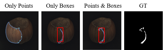
Figure 3: The results produced by SAM with different spatial prompts. As we can see, constraining SAM with the spatial prompt that represents points and boxes as a whole leads to better results.

With the rough segmentation $O$ from the CLIP phase, we propose the Multi-level Mask Refinement (MMR) module to extract point and box prompts to guide SAM to generate accurate masks. In the MMR module, the foreground of the rough segmentation, denoted as $O_{f}\in\mathbb{R}^{H\times W}$, is firstly post-processed with a binarization step to obtain a binary mask ${O_{b}(x,y)}$. Denote $v(x,y)_{f},x\in{H},y\in{W}$ as the value of a specific pixel in $O_{f}$, then the value of each pixel $v(x,y)_{b}$ in ${O_{b}(x,y)}$ can be calculated as:

$$v(x,y)_{b}=\begin{cases}&1,\text{if }v(x,y)_{f}>threshold\\ &0,otherwise\end{cases}$$ (7)

where $threshold$ represents the binary threshold, and the value 1 corresponds to the anomalous pixels. Within the connected areas of this binary mask, we identify some boxes and points to provide spatial prompts for SAM. For point selection, $m$ random points are chosen, represented as $S_{p}=[(x_{p_{1}},y_{p_{1}}),\dots,(x_{p_{m}},y_{p_{m}})]$, where $(x_{p_{i}},y_{p_{i}})$ represents the position of the i-th point. Boxes are generated based on the size of connected regions in the binary mask, with the i-th box denoted by $S_{b_{i}}=[(x_{b_{i}},y_{b_{i}},h_{b_{i}},w_{b_{i}})]$. The complete set with $q$ boxes is represented as $S_{b}=[S_{b_{1}},\dots,S_{b_{q}}]$.

With the point prompts $S_{p}$ and box prompts $S_{b}$, we explore the optimal prompt sets for SAM. As can be seen in Figure 3, employing either points or boxes alone leads to biased results. In contrast, the combined application of both points and boxes can yield more precise and detailed segmentation. Therefore, in our ClipSAM framework, we use $S=S_{b}\cup{S_{p}}$ as the prompt set for SAM. With the original image $I$ and spatial prompts $S$ as inputs, SAM generates encoded features ${z}_{i}$ and ${z}_{s}$. The decoder within SAM then outputs the refined masks and corresponding confidence scores:

$$({masks},{scores})=\mathbb{D}^{sam}({z}_{i}\mid{z}_{s}).$$ (8)

Each box shares the same point constraints, resulting in $q$ distinct segmentation masks. In our ClipSAM framework, SAM is configured to produce three masks with varying confidence scores for each box, represented as $masks=[(m_{1}^{1},m_{1}^{2},m_{1}^{3});\dots;(m_{q}^{1},m_{q}^{2},m_{q}^{3})]$ and $scores=[(s_{1}^{1},s_{1}^{2},s_{1}^{3});\dots;(s_{q}^{1},s_{q}^{2},s_{q}^{3})]$. The final fine-grained segmentation result $O_{final}$ is obtained by normalizing the fusion of rough segmentation and the refined masks:

$$O_{final}=Norm(O+\sum_{i=1}^{q}\sum_{j=1}^{3}m_{i}^{j}\times s_{i}^{j}).$$ (9)

3.4 Objective Function

In our ClipSAM framework, the only part involving training is the UMCI module. To effectively optimize this module, we employ the Focal Loss Lin et al. (2017) and the Dice Loss Milletari et al. (2016), both of which are well-suited for segmentation tasks.

Focal Loss. Focal loss is primarily applied to address class imbalance problem, a common challenge in segmentation tasks. It is appropriate for anomaly segmentation because, usually, the anomaly merely occupies a small fraction of the entire object. The expression of Focal loss is:

$$l_{focal}=-\frac{1}{H\times W}\textstyle\sum_{i=0}^{H\times W}(1-p_{i})^{\gamma}\log{(p_{i})},$$ (10)

where $p_{i}$ is the predicted probability for a pixel being abnormal, and $\gamma$ is a tunable parameter and set to 2 in our paper.

Dice Loss. Dice Loss calculates a score based on the overlap between the target area and the model’s output. This metric is also effective for class imbalance issue. Dice Loss can be calculated as:

$$l_{dice}=1-\frac{1}{N}\frac{2\times{\textstyle\sum_{i=1}^{N}}y_{i}\hat{y}_{i}}{{\textstyle\sum_{i=1}^{N}}y_{i}^{2}+{\textstyle\sum_{i=1}^{N}}\hat{y}_{i}^{2}},$$ (11)

where $N=H\times W$ is the total number of pixels in features.

Total Loss. We set separate loss weights for each stage and the total loss can be expressed as:

$$l_{all}=\textstyle\sum_{i=1}^{n}\lambda_{i}(l_{focal}^{i}+l_{dice}^{i}),$$ (12)

where $i$ denotes the index of stages, $\lambda_{i}$ is the loss weight of the i-th stage. The CLIP encoder in our implementation consists of 4 stages in total, and we set the loss weights for these stages at $0.1$, $0.1$, $0.1$, and $0.7$ respectively.

4 Experiments

		MVTec-AD				VisA
Base model	Method	AUROC	$F_{1}$-max	AP	PRO	AUROC	$F_{1}$-max	AP	PRO
CLIP-based Approaches	WinCLIP	85.1	31.7	-	64.6	79.6	14.8	-	56.8
	APRIL-GAN	87.6	43.3	40.8	44.0	94.2	32.3	25.7	86.8
	SDP	88.7	35.3	28.5	79.1	84.1	16.0	9.6	63.4
	SDP+	91.2	41.9	39.4	85.6	94.8	26.5	20.3	85.3
SAM-based Approaches	SAA	67.7	23.8	15.2	31.9	83.7	12.8	5.5	41.9
	SAA+	73.2	37.8	28.8	42.8	74.0	27.1	22.4	36.8
CLIP & SAM	ClipSAM(Ours)	92.3	47.8	45.9	88.3	95.6	33.1	26.0	87.5

Table 1: Performance comparison of different kinds of ZSAS approaches on the MVTec-AD and VisA datasets. Evaluation metrics include AUROC, $F_{1}$-max, AP, and PRO. Bold indicates the best results.

4.1 Experimental Setup

Datasets. In this study, we conduct experiments on two commonly-used datasets of industrial anomaly detection, namely VisA Zou et al. (2022) and MVTec-AD Bergmann et al. (2019), which encompass a diverse range of industrial objects categorized as normal or abnormal. We follow the same training setup as existing zero-shot anomaly segmentation studies Jeong et al. (2023); Chen et al. (2023a) to evaluate the performance of our method. Specifically, the model is first trained on the MVTec-AD dataset and then tested on the VisA dataset, and vice versa. Additional experimental results on other datasets are provided in Appendix C.

Metrics. Following Jeong et al. (2023), we employ widely-used metrics, i.e., AUROC, AP, $F_{1}$-max, and PRO Bergmann et al. (2020), to provide a fair and comprehensive comparison with existing ZSAS methods. Specifically, AUROC reflects the model’s ability to distinguish between classes at various threshold levels. AP quantifies the model’s accuracy across different levels of recall. $F_{1}$-max is the harmonic mean of precision and recall at the optimal threshold, implying the accuracy and coverage of the model. PRO assesses the proportion of correctly predicted pixels within each connected anomalous region, offering insights into the model’s local prediction accuracy. Higher values of these metrics mean better performance of the evaluated method.

Implementation details. In the experiments, the pre-trained ViT-L-14-336 model released by OpenAI, which consists of 24 Transformer layers, is utilized for CLIP encoders. We extracted the image patch tokens after each stage of the image encoder (i.e., layers 6, 12,18, and 24) for the training of our proposed UMCI module, respectively. The optimization process is conducted on a single NVIDIA 3090 GPU using AdamW optimizer with the learning rate of ${1\times 10^{-4}}$ and the batch size of 8 for 6 epochs. For SAM, we use the ViT-H pre-trained model.

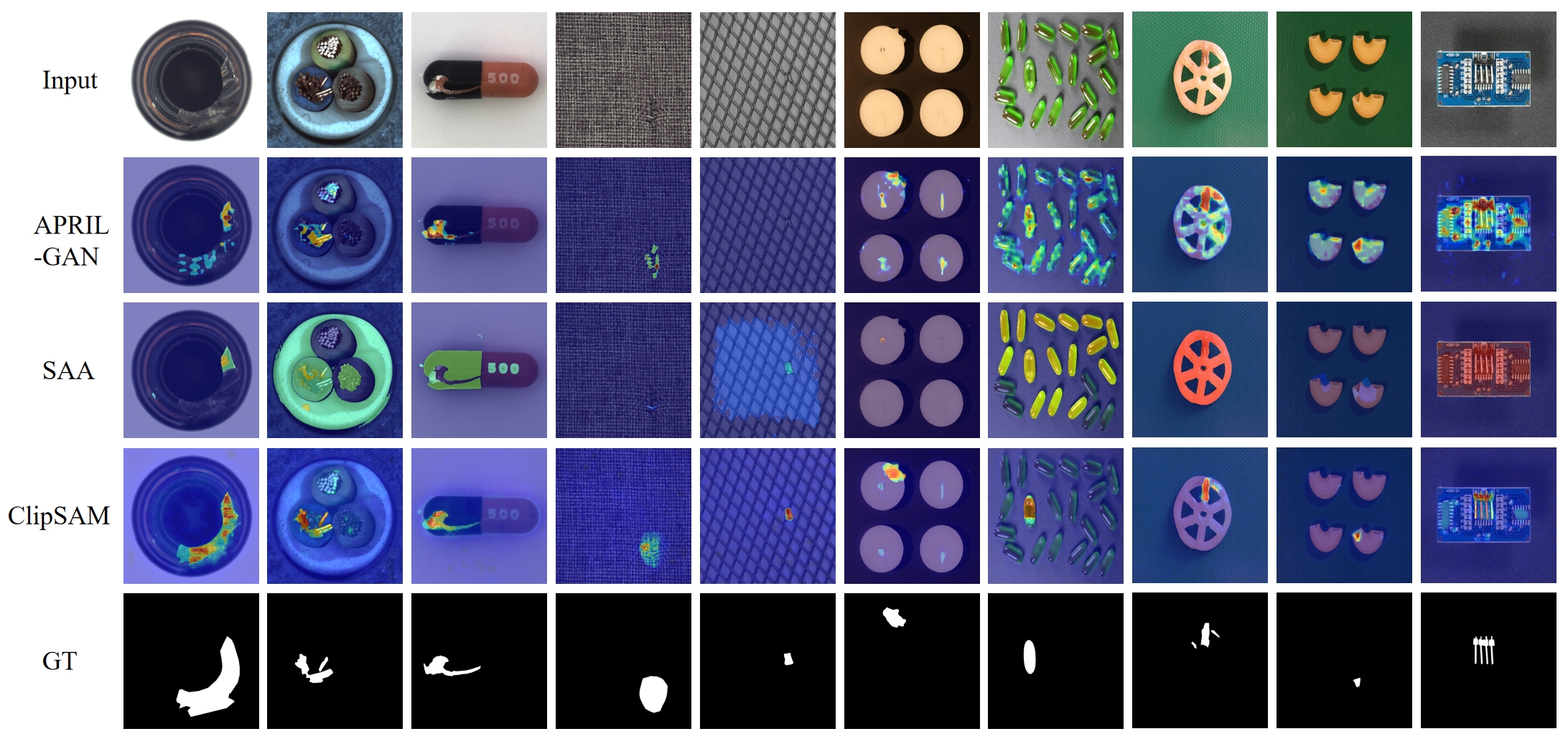
Figure 4: Comparison of visualization results among ClipSAM, CLIP-based, and SAM-based methods on the MVTec-AD dataset. Our ClipSAM performs much better on the location and boundary of the anomaly segmentation.

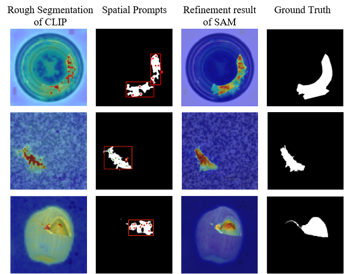
Figure 5: Visualization of the results of each step of our ClipSAM collaboration framework. ClipSAM first uses CLIP for rough segmentation and then uses SAM for refinement.

4.2 Experiments on MVTec-AD and VisA

Comparison with state-of-the-art approaches. In this section, we evaluate the effectiveness of our proposed ClipSAM framework for ZSAS on the MVTec-AD and VisA datasets. Table 1 shows the comprehensive comparison between our proposed ClipSAM and the state-of-the-art ZSAS methods Jeong et al. (2023); Chen et al. (2023a); Cao et al. (2023); Chen et al. (2023b) on different datasets and various metrics. It can be concluded that our proposed ClipSAM outperforms existing state-of-the-art methods in all four metrics. Taking the MVTec-AD dataset as an example, our proposed ClipSAM outperforms the advanced CLIP-based method SDP+ by 1.1%, 5.9%, 6.5% and 2.7% on the AUROC, $F_{1}$-max, AP and PRO metrics respectively. Compared to the SAM-based approach, our method exhibits superior performance benefits, i.e., improvements of 19.1%, 10.0%, 17.1%, and 45.5% for the metrics. On the VisA dataset, our proposed method similarly shows an overall performance enhancement, demonstrating the effectiveness and generalization of our ClipSAM.

Qualitative comparisons. We provide some visualization of ZSAS results in Figure 4 to further demonstrate the effectiveness of the proposed method. For comparison, we also show the segmentation visualization of APRIL-GAN (CLIP-based method) and SAA (SAM-based method). It can be observed that APRIL-GAN can roughly locate the anomalies but fails to provide excellent segmentation results. In contrast, SAA can perform the segmentation well but cannot cover the anomalous region accurately. Compared with these methods, our proposed ClipSAM provides accurate localization as well as good segmentation results. More visualization results are provided in Appendix D. To better understand the role of each module in the ClipSAM framework, we also visualize the rough segmentation results of the CLIP phase and the processed prompts fed into the SAM phase in Figure 5. It shows that CLIP performs a rough segmentation of abnormal parts and generates corresponding prompts based on their locations to complete SAM’s further refinement of the results. Please refer to Appendix E for more details.

Components of ClipSAM		AUROC	$F_{1}$-max	AP	PRO
UMCI	only w/strip	90.8	44.3	34.9	79.6
	only w/scale	90.9	44.4	42.7	81.9
Module	w/o UMCI	60.4	19.7	25.0	34.7
	w/o MMR	91.8	46.7	44.7	84.8
ClipSAM(Ours)		92.3	47.8	45.9	88.3

Table 2: Ablation study of different components in our ClipSAM framework on MVTec-AD dataset. Bold indicates the best results.

Hyperparameters		AUROC	$F_{1}$-max	AP	PRO
Hidden dim ($c_{h}$)	194	91.8	45.6	43.8	83.1
	256	91.7	46.4	44.6	83.6
	384	92.3	47.8	45.9	88.3
Kernel size ($s_{1}$ & $s_{2}$)	2 & 4	91.9	45.7	45.3	85.1
	3 & 9	92.3	47.8	45.9	88.3
	6 & 10	91.8	46.8	44.7	84.9
Threshold ($thr$)	0.45	91.5	43.3	44.9	82.5
	0.47	92.3	47.8	45.9	88.3
	0.50	91.7	44.6	43.4	83.2

Table 3: Ablation study of different hyperparameters used in our ClipSAM framework on MVTec-AD dataset. Bold indicates the best results in the UMCI module. $c_{h}$ represents the hidden dimension of the convolutional layer. $s_{i}$ denotes the kernel size of the average pooling layer used in the scale path. $thr$ means the threshold for binarization.

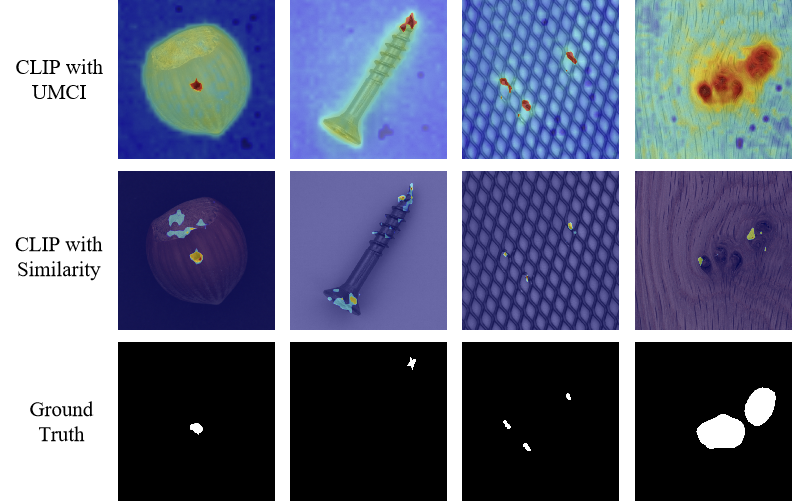
Figure 6: Visualization of anomaly localization and rough segmentation by CLIP with the UMCI module and CLIP with similarity calculation.

4.3 Ablation Studies

In this section, we conduct several ablation studies on the MVTec-AD dataset to further explore the effect of different components and the experiment settings on the results in the proposed ClipSAM framework.

Effect of components. Table 2 shows the results of the ablation study of different components in ClipSAM. Specifically, we first explore the impact of preserving only the strip path or the scale path in the UMCI module. Subsequently, the performance of removing either the UMCI or MMR module from the framework is tested. It can be found that removing a path in the UMCI module can lead to performance degradation, and removing the scale path has a greater impact, reflecting the necessity of combining two paths in the UMCI module. At the module level, removing the MMR module will slightly lower performance. Comparing this result with SDP+, we can surprisingly find that the rough segmentation results of the CLIP phase yield even better performance than CLIP-based methods. Figure 6 shows the visualization comparison between the rough segmentation and APRIL-GAN (Since SDP is not open source). The first two columns of Figure 6 indicates that UMCI can locate the anomalies more accurately, and the last two columns shows that UMCI provides better segmentation. In comparison with the MMR module, removing the UMCI module means regarding the similarity-based segmentation as the rough segmentation result. However, as shown in Figure 4, the similarity-based segmentation cannot provide text-aligned patch tokens and accurate local spatial prompts for the subsequent MMR module. This results in a performance collapse, which demonstrates the important role of the UMCI module in the ClipSAM framework.

Effect of hyperparameters. We explore the effects of various hyperparameters on our ClipSAM framework and record the results in Table 3. An analysis of the roles of each hyperparameter in the ClipSAM framework is provided based on the results. Hidden Dimension (${c_{h}}$) determines the output feature dimension of the convolution layer. Larger ${c_{h}}$ values contribute to the effective interpretation of visual features by the model. Kernel size (${s_{i}}$) affects the size of multi-scale visual features, which should be moderate to provide easy-to-understand visual context. Threshold Value ($thr$) primarily impacts the initial binarized segmentation of the SAM phase. The setting of $thr$ should also be moderate: a small value may cause the non-anomalous regions to be misclassified and thus unable to generate accurate masks for SAM; a large value may cause some anomalies to be ignored and not detected.

5 Conclusion

We propose the CLIP and SAM Collaboration (ClipSAM) framework to solve zero-shot anomaly segmentation for the first time. To cascade the two foundation models effectively, we introduce two modules. One is the UMCI module, which explicitly reasons anomaly locations and achieves rough segmentation. The other is the MMR module, which refines the rough segmentation results by employing the SAM with precise spatial prompts. Sufficient experiments showcase that ClipSAM provides a new direction for improving ZSAS by leveraging the characteristics of different foundation models. In future work, we will further investigate how to integrate knowledge from different models to enhance the performance of zero-shot anomaly segmentation.

Appendix A Text design

Figure 7: Lists of multi-level prompts considered in this paper to construct compositional prompt ensemble. The integrated descriptive statements are primarily categorized into phrases that describe both normal and abnormal states and templates. The category names are illustrated using the MVTec-AD dataset as example.

As shown in Figure 7, the prompt design in ClipSAM follows the same approach in WinCLIP Jeong et al. (2023). Specifically, for a given category, such as ’bottle’ in the MVTec-AD dataset, phrases describing the normal state, like ”perfect bottle”, are combined using the category name. Subsequently, these phrases describing the normal state are integrated separately with the prompt templates. This process can yield multiple descriptive statements about a normal bottle, such as ”a photo of a perfect bottle.” Assuming we have $m$ prompt templates and $n$ phrases describing normal states, we can generate a total of ${m\times n}$ sentences to describe a normal ’bottle’. To obtain text features corresponding to each sentence, we utilize the text encoder of CLIP and then compute the average of all text features that describe normality. This yields $L_{normal}\in\mathbb{R}^{c_{t}\times 1}$. Here, $c_{t}$ represents the feature dimension, and $1$ denotes the text category, namely normal. Similarly, we can calculate the averaged feature $L_{anomaly}\in\mathbb{R}^{c_{t}\times 1}$ for sentences describing anomalies. Finally, we concatenate $L_{normal}$ and $L_{anomaly}$ on the category dimension to obtain $L\in\mathbb{R}^{c_{t}\times 2}$, where $2$ represents the two categories, normal and abnormal.

During the training and testing processes, it is assumed that the object categories are known, while the specific anomaly categories are unknown. Consequently, for a batch of data, text features corresponding to their respective categories can be generated based on the known object categories. In situations where the categories are unknown, the placeholder ’object’ can be used to substitute for specific object categories, which has been proven effective in experiments Zhou et al. (2023).

Appendix B Strip path and Scale path

The UMCI module consists of two parallel paths: the $Strip$ $Path$ and the $Scale$ $Path$. The $Strip$ $Path$ employs interactions between language features and row- and column-level visual features to calculate visually salient pixels with the strongest language perception in different directions. The $Scale$ $Path$ utilizes interactions between language features and globally visual features at different scales to comprehend what is considered anomaly.

Algorithm 1 Strip Path

Input: Image patch token $P$, Language feature $L$;
Output: strip path output $M_{row,col}$

1:  $\hat{P}=Linear(P)$.

2:  $v_{row}=conv_{1\times 3}(Avg\_Pool_{1\times W}(\hat{P}))$, $v_{col}=conv_{3\times 1}(Avg\_Pool_{H\times 1}(\hat{P}))$,

3:  for  $i$ in $(row,col)$ do

4:     $t_{i}^{1}=conv_{1\times 1}^{1}(L)$,$t_{i}^{2}=conv_{1\times 1}^{2}(L)$,$t_{new}=GRU(Attention(t_{i}^{1},v_{i},v_{i}))$,$v_{i}^{att}=Attention(v_{i},t_{new},t_{i}^{2})$,$M_{i}=Norm(v_{i}^{att}+v_{i})$,

5:  end for

6:  $M_{row,col}=conv_{3\times 3}(B(M_{row})+B(M_{col}))$

7:  return $M_{row,col}$

Algorithm 2 Scale Path

Input: Image patch token $P$, Language feature $L$;
Output: strip path output $M_{{g}_{1},{g}_{2}}$

1:  $\hat{P}=Linear(P)$.

2:  $v_{{g}_{1}}=conv_{3\times 3}^{{g}_{1}}(Avg\_Pool_{{s}_{1}\times{s}_{1}}(\hat{P}))$, $v_{{g}_{2}}=conv_{3\times 3}^{{g}_{2}}(Avg\_Pool_{{s}_{2}\times{s}_{2}}(\hat{P}))$,

3:  for  $i$ in $({g}_{1},{g}_{2})$ do

4:     $t_{i}^{k}=conv_{1\times 1}^{k}(L)$ , $t_{i}^{v}=conv_{1\times 1}^{v}(L)$,$v_{i}^{att}=Attention(v_{i},text_{i}^{k},text_{i}^{v})$,$M_{i}=Norm(v_{i}^{att}+v_{i})$,

5:  end for

6:  $M_{{g}_{1},{g}_{2}}=conv_{3\times 3}^{{g}_{1},{g}_{2}}(B(M_{{g}_{1}})+B(M_{{g}_{2}}))$

7:  return $M_{{g}_{1},{g}_{2}}$

(1) ${Strip}$ ${Path}$. The interaction conducted by the strip path involves the fusion of text features and row-and-column visual features. Specifically, visual features are aggregated into row-level and column-level features from horizontal and vertical directions through average pooling layers. Taking row-level features $v_{row}$ as an example, text features $L$ are processed by convolutional layers to obtain language features $t_{row}^{1}$, $t_{row}^{2}$ with dimensions matching the visual features. Subsequently, a two-stage attention mechanism is employed to perceive relevant language features at each pixel of the row-level features. In the attention computation process, we employ the Scaled Dot-Product Attention mechanism Vaswani et al. (2017):

$$Attention(Q,K,V)=softmax(\frac{QK^{T}}{\sqrt{d_{k}}})V.$$ (13)

As shown in Figure 8, the first attention step is designed to capture the correlated visual features corresponding to each language feature. Then we use GRU  Cho et al. (2014) to merge the learned visual features with the original language features, which we can obtain language features enriched with visual information. Taking this new language feature, original visual and language features as K, Q, V respectively for attention computation can effectively aggregating features. Finally, we use the residual method to add $v_{row}$ to the result and get $M_{row}\in\mathbb{R}^{H\times c_{h}}$:

$$t_{new}=GRU(Attention(t_{row}^{1},v_{row},v_{row})),$$ (14)

$$v_{row}^{att}=Attention(v_{row},t_{new},t_{row}^{2}),$$

$$M_{row}=Norm(v_{row}^{att}+v_{row}),$$

where ${Norm}$ denotes L2 regularization. Please refer to Algorithm 1 for specific content.

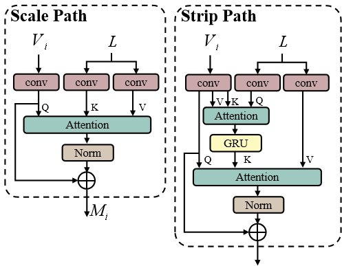
Figure 8: Diagram depicting the attention calculation process in the strip path and scale path.

(2) ${Scale}$ ${Path}$. The scale path is utilized for the interaction between text and multi-scaled visual features. Initially, visual features at different scales are obtained through average pooling layers with different kernel sizes. Taking one of these scales as an example, convolutional layers are employed to process text features to match the feature dimensions. Subsequently, a dedicated attention mechanism is employed for cross-modal interaction to obtain $M_{g_{1}}\in\mathbb{R}^{h_{g_{1}}\times w_{g_{1}}\times c_{h}}$. The residual connection is also used here to add the original vision and the result. The specific formula is as follows:

$$v_{{g}_{1}}^{att}=Attention(v_{{g}_{1}},text_{{g}_{1}}^{k},text_{{g}_{1}}^{v}),$$ (15)

$$M_{{g}_{1}}=Norm(v_{{g}_{1}}^{att}+v_{{g}_{1}}),$$

Please refer to Algorithm 2 for specific content.

It is worth noting that all convolutional layers in the UMCI module are independent of each other.

		MTD				KSDD2
Base model	Method	AUROC	$F_{1}$-max	AP	PRO	AUROC	$F_{1}$-max	AP	PRO
CLIP-based Approaches	APRIL-GAN	51.1	16.6	9.8	17.2	52.1	10.7	9.3	13.3
SAM-based Approaches	SAA+	69.4	37.3	28.8	-	77.5	61.6	49.6	-
CLIP & SAM	ClipSAM(Ours)	88.0	55.2	51.9	71.3	90.7	67.2	67.9	88.8

Table 4: Performance comparison of different kinds of ZSAS approaches on the MTD and KSDD2 datasets. Evaluation metrics include AUROC, $F_{1}$-max, AP, and PRO. Bold indicates the best results.

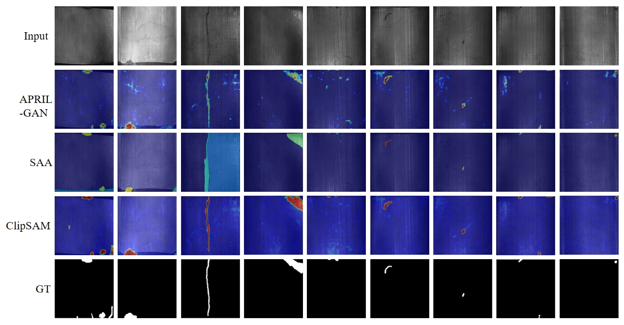
Figure 9: Comparison of visualization results among ClipSAM, CLIP-based, and SAM-based methods on the MTD dataset. Our ClipSAM performs much better on the location and boundary of the anomaly segmentation.

Appendix C Additional experiments on more datasets

We validated the effectiveness of ClipSAM on two commonly used datasets for zero-shot anomaly segmentation, namely MVTec-AD Bergmann et al. (2019) and ViSA Zou et al. (2022). Additionally, we conducted relevant experiments on the MTD Huang et al. (2020) and KSDD2 Božič et al. (2021) datasets to further confirm the generalizability of our approach.

C.1 MVTec-AD

The MVTec-AD dataset serves as an unsupervised anomaly detection dataset, comprising a total of 3466 unlabeled images and 1888 annotated images with pixel-level segmentation annotations. The image sizes are either 700×700 or 1024×1024 pixels. The training dataset consists of 3629 images, all depicting defect-free instances. The test dataset comprises 1725 images, including both defective and defect-free samples. The dataset encompasses 15 categories, comprising 5 texture categories such as carpets and leather, and 10 object categories including bottles, cables, capsules, chestnuts, and others. In total, the dataset contains 73 types of anomalies, such as scratches, dents, and missing parts. Standard evaluation metrics, including AUROC, AP, $F_{i}$-max and PRO are commonly employed for assessment.

C.2 VisA

The VisA dataset is also one of the commonly used datasets for zero-shot anomaly segmentation. It consists of 10,821 images, comprising 9,621 normal samples and 1,200 anomaly samples. The dataset is organized into 12 subsets, each corresponding to a different object category. Among them, four subsets represent different types of printed circuit boards (PCBs) with relatively complex structures, including transistors, capacitors, chips, and other components. Additionally, four subsets (Capsules, Candles, Macaroni1, and Macaroni2) contain multiple instances in their views. Instances in Capsules and Macaroni2 exhibit significant variations in both position and orientation. The performance of the model on this dataset can also be evaluated using AUROC, AP, $F_{i}$-max and PRO.

C.3 MTD

The Magnetic Tile Defect (MTD) dataset is a more specialized dataset that consists of images related to a single object category but with various defect categories. It encompasses six common defect types in magnetic tiles, such as blowhole, break, crack, and others. The dataset comprises a total of 925 images without defects and 392 images with anomalies, each with corresponding image annotations. Performance evaluation can be conducted using the AUROC, AP, $F_{i}$-max and PRO metrics in a similar manner.

C.4 KSDD2

The Kolektor Surface-Defect Dataset 2 (KSDD2) is relevant to industrial quality inspection and can also be used for anomaly segmentation. It comprises 356 images with obvious defects and 2979 images without any defects. The dimensions of each image in the dataset are approximately 230×630 pixels. The dataset is divided into a training set and a test set, with the training set consisting of 246 positive images and 2085 negative images, while the test set includes 110 positive images and 894 negative images. The dataset encompasses various types of defects, including scratches, small spots, surface defects, and others. The performance of the model in zero-shot anomaly segmentation on this dataset can also be assessed using the AUROC, $F_{1}$-max, AP, and PRO metrics.

C.5 Experimental results

Implementation details. Our experiments adhere to the settings defined in AnomalyCLIP Zhou et al. (2023). Specifically, the model is trained on the MVTec-AD dataset and tested on the MTD and KSDD2 datasets. For the MTD dataset, all data samples are considered as the test set. In the case of the KSDD2 dataset, we directly utilize its test set.

In the experiments, the pre-trained ViT-L-14-336 model released by OpenAI, which consists of 24 Transformer layers, is utilized for CLIP encoders. We extracted the image patch tokens after each stage of the image encoder (i.e., layers 6, 12,18, and 24) for the training of our proposed UMCI module, respectively. The optimization process is conducted on a single NVIDIA 3090 GPU using AdamW optimizer with the learning rate of ${1\times 10^{-4}}$ and the batch size of 8 for 6 epochs. For SAM, we use the ViT-H pre-trained model.

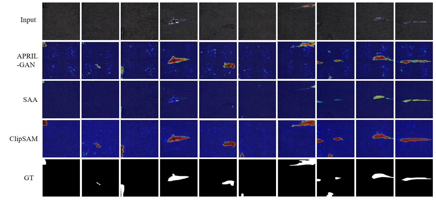
Figure 10: Comparison of visualization results among ClipSAM, CLIP-based, and SAM-based methods on the KSDD2 dataset. Our ClipSAM performs much better on the location and boundary of the anomaly segmentation.

Comparison with state-of-the-art approaches. Due to the fact that CLIP-based methods such as SDP Chen et al. (2023b) are not open source and have not been experimentally evaluated on the MTD and KSDD2 datasets, no comparison is provided here. Therefore, we evaluate the performance of the CLIP-based method APRIL-GAN Chen et al. (2023a), the SAM-based method SAA Cao et al. (2023), and our proposed ClipSAM on the zero-shot anomaly segmentation task. As shown in Table 4, our method demonstrates significant improvements over the other two methods across different metrics. In particular, taking the MTD dataset as an example, when compared to APRIL-GAN, ClipSAM demonstrates improvements of 36.9% in AUROC, 38.6% in $F_{1}$-max, 42.1% in AP, and 54.1% in PRO. When contrasted with SAA+, ClipSAM shows enhancements of 18.6% in AUROC, 17.9% in $F_{1}$-max, and 23.1% in AP. Additionally, ClipSAM also demonstrates remarkable performance advantages on the KSDD2 dataset.

Qualitative comparisons. We further visualize the experimental results on the MTD dataset and KSDD2 dataset in Figure 9 and Figure 10. The compared methods include APRIL-GAN Chen et al. (2023a) (CLIP-based method), SAA Cao et al. (2023) (SAM-based method), and ClipSAM. Similar conclusions can be observed from both figures, indicating that ClipSAM outperforms the other two methods in terms of localization and segmentation capabilities. Meanwhile, APRIL-GAN and SAA exhibit similar disadvantages on both datasets. Specifically, the CLIP-based method, although capable of roughly locating the position of defects guided by language, suffers from inaccurate segmentation areas. Additionally, unexpected high predictions occur outside the real masks, as shown in the third and fifth columns of Figure 9. This is attributed to misalignment between image patch tokens and text tokens, resulting in erroneous predictions and a decrease in performance.

Furthermore, while the SAM-based method demonstrates good segmentation performance, it generates incorrect segmentation masks due to the use of ambiguous positional information words as prompts. In particular, in the third column of Figure 9, SAA produces large-area erroneous masks, and in the eighth column of Figure 10, SAA misses parts of the masks. In contrast, ClipSAM performs well on the entire dataset, accurately locating anomalous positions and generating precise segmentation masks without exhibiting errors in unexpected locations, as seen in APRIL-GAN.

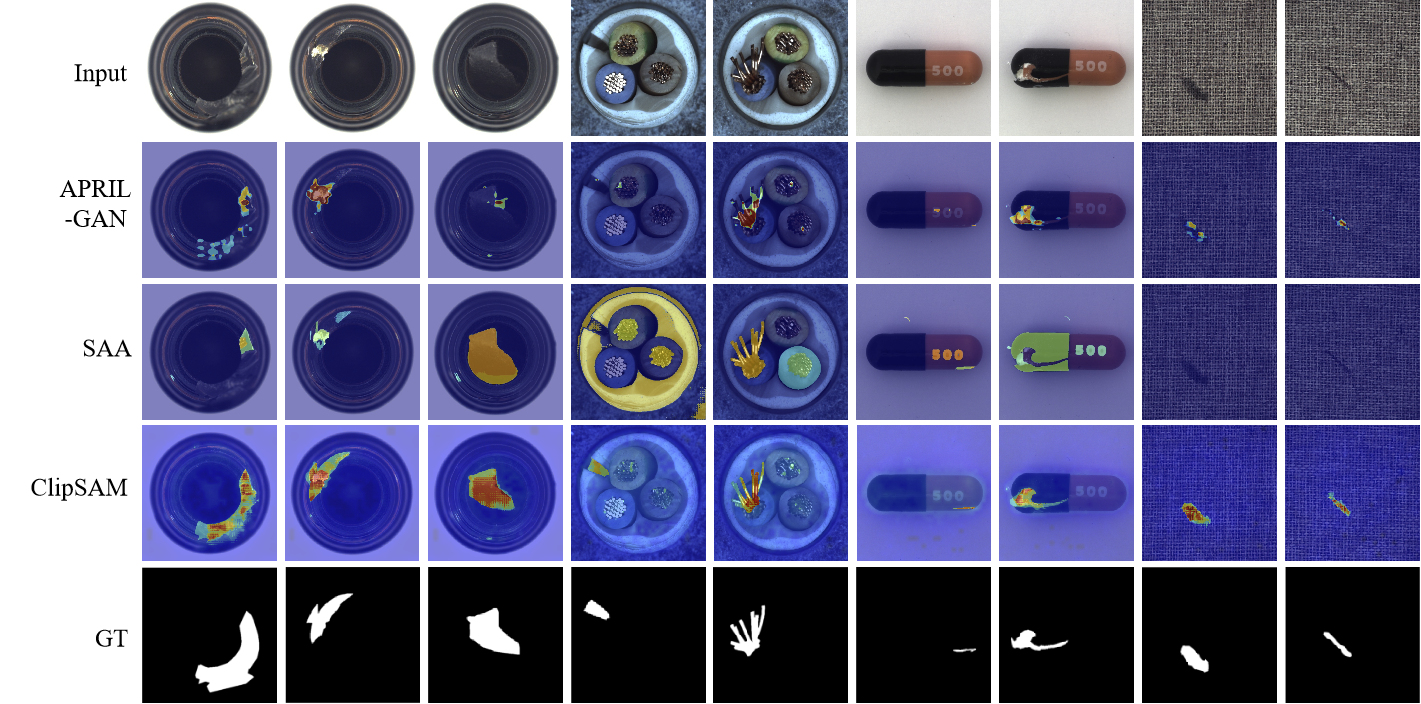
Figure 11: Comparison of visualization results among ClipSAM, CLIP-based, and SAM-based methods on the MVTec-AD dataset. Our ClipSAM performs much better on the location and boundary of the anomaly segmentation.

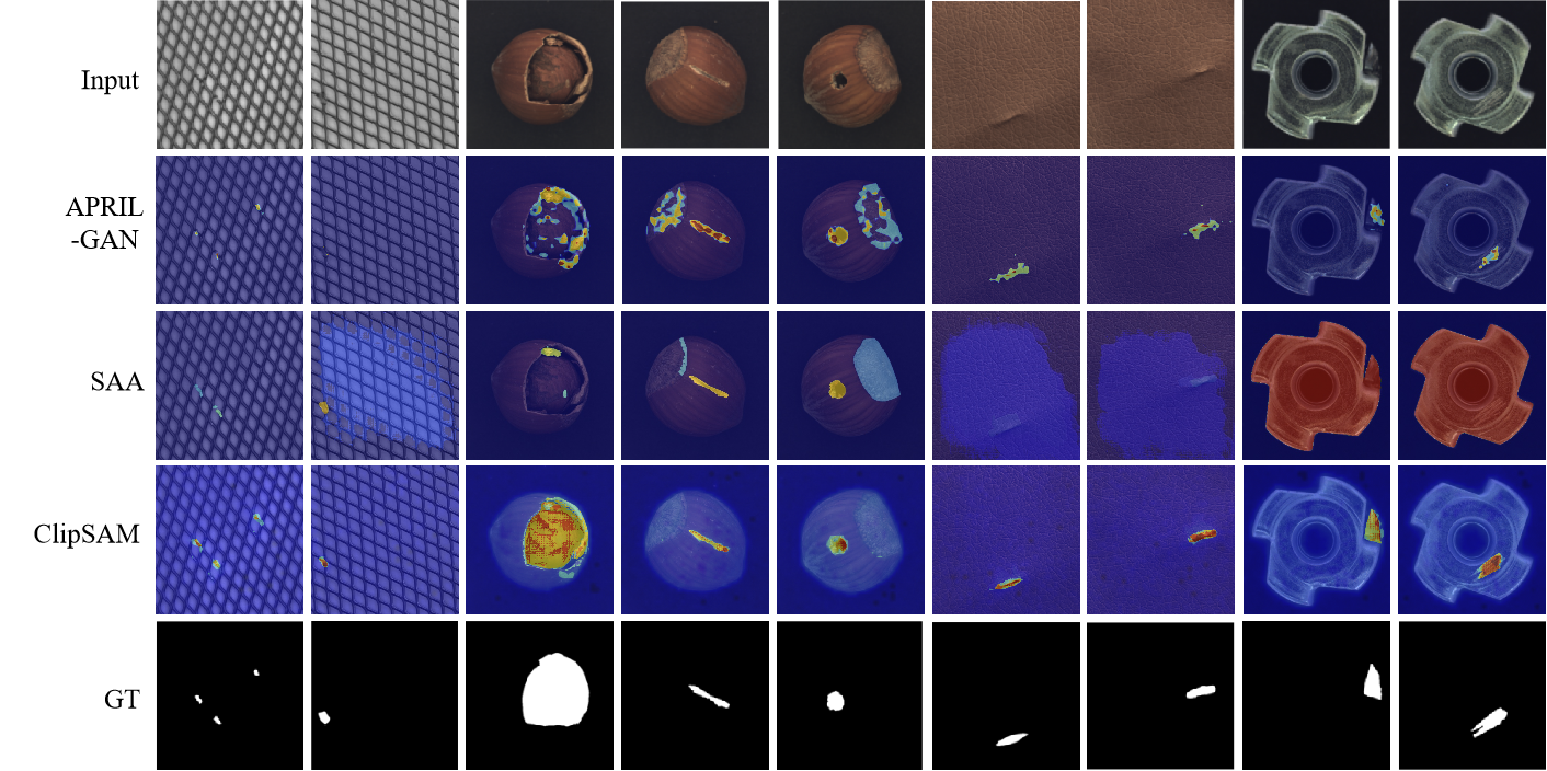
Figure 12: Comparison of visualization results among ClipSAM, CLIP-based, and SAM-based methods on the MVTec-AD dataset. Our ClipSAM performs much better on the location and boundary of the anomaly segmentation.

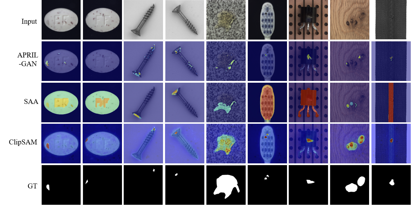
Figure 13: Comparison of visualization results among ClipSAM, CLIP-based, and SAM-based methods on the MVTec-AD dataset. Our ClipSAM performs much better on the location and boundary of the anomaly segmentation.

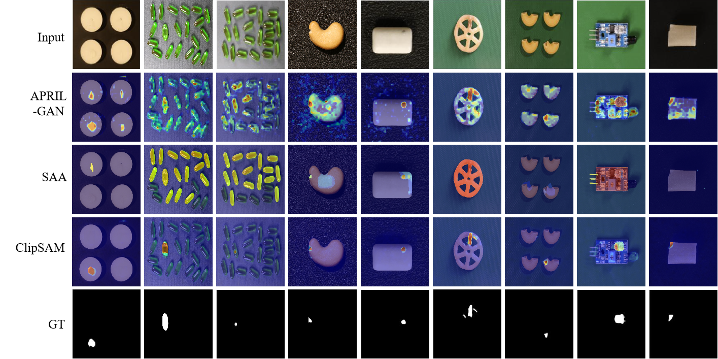
Figure 14: Comparison of visualization results among ClipSAM, CLIP-based, and SAM-based methods on the VisA dataset. Our ClipSAM performs much better on the location and boundary of the anomaly segmentation.

Appendix D Additional visualization

In this section, we visualize the anomaly segmentation results of the proposed ClipSAM framework on the MVTec-AD dataset and the VisA dataset. Figure 11,  12,  13,  14 illustrate the visual comparisons between APRIL-GAN Chen et al. (2023a) (CLIP-based method), SAA Cao et al. (2023) (SAM-based method), and our ClipSAM method. Clearly, our ClipSAM demonstrates stronger understanding of anomalous regions, benefiting from the designed UMCI and MMR modules. The process of rough segmentation by CLIP followed by refinement using SAM successfully mitigates misdetections and omissions of certain anomalies.

Specifically, CLIP-based methods tend to incorrectly classify regions outside actual anomaly areas as anomalies. Even when identifying anomaly locations, their segmentation results often deviate significantly from the ground truth labels. On the other hand, SAM-based methods heavily rely on post-processing steps for masks. While the initial candidate masks may contain correct masks, complex filtering can introduce substantial biases. Additionally, due to the vague semantic descriptions guiding the model’s attention, SAM might focus on parts outside the anomaly regions and segment them entirely, as shown in the fourth column of Figure 11. In reality, anomalies usually constitute a small portion of the entire object, and such errors can significantly impact the results.

Observing the figures, APRIL-GAN tends to identify anomaly locations, though less accurately. SAM provides accurate segmentation of components but lacks precise constraints, leading to significant deviations in results. In contrast, ClipSAM’s two-stage strategy effectively combines the strengths of CLIP and SAM, resulting in better performance in zero-shot anomaly segmentation.

Appendix E Two-stage visualization

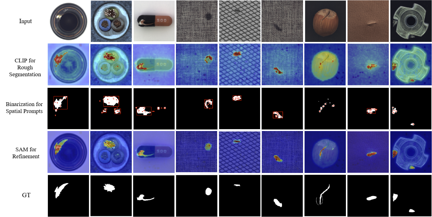
Figure 15: Visualization of different stages (the process of localization and rough segmentation by CLIP followed by result refinement through SAM) under the ClipSAM framework on the MVTec-AD dataset.

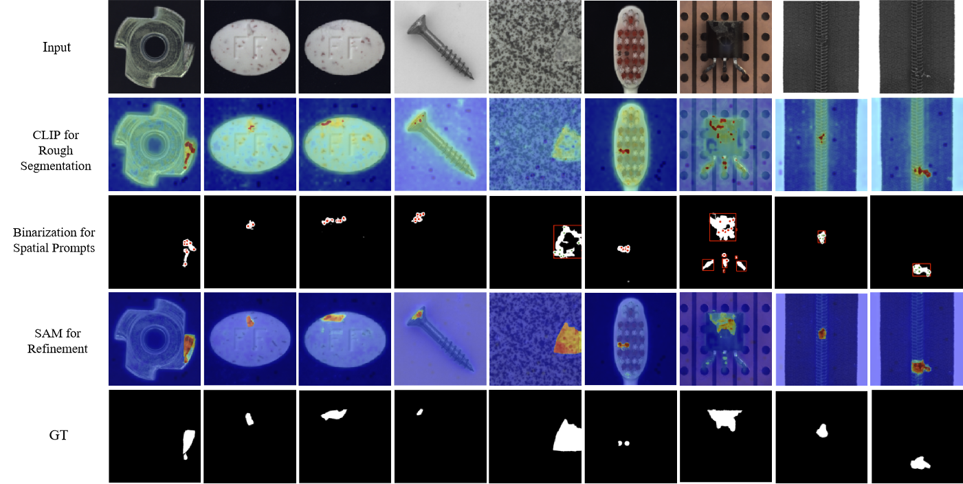
Figure 16: Visualization of different stages (the process of localization and rough segmentation by CLIP followed by result refinement through SAM) under the ClipSAM framework on the MVTec-AD dataset.

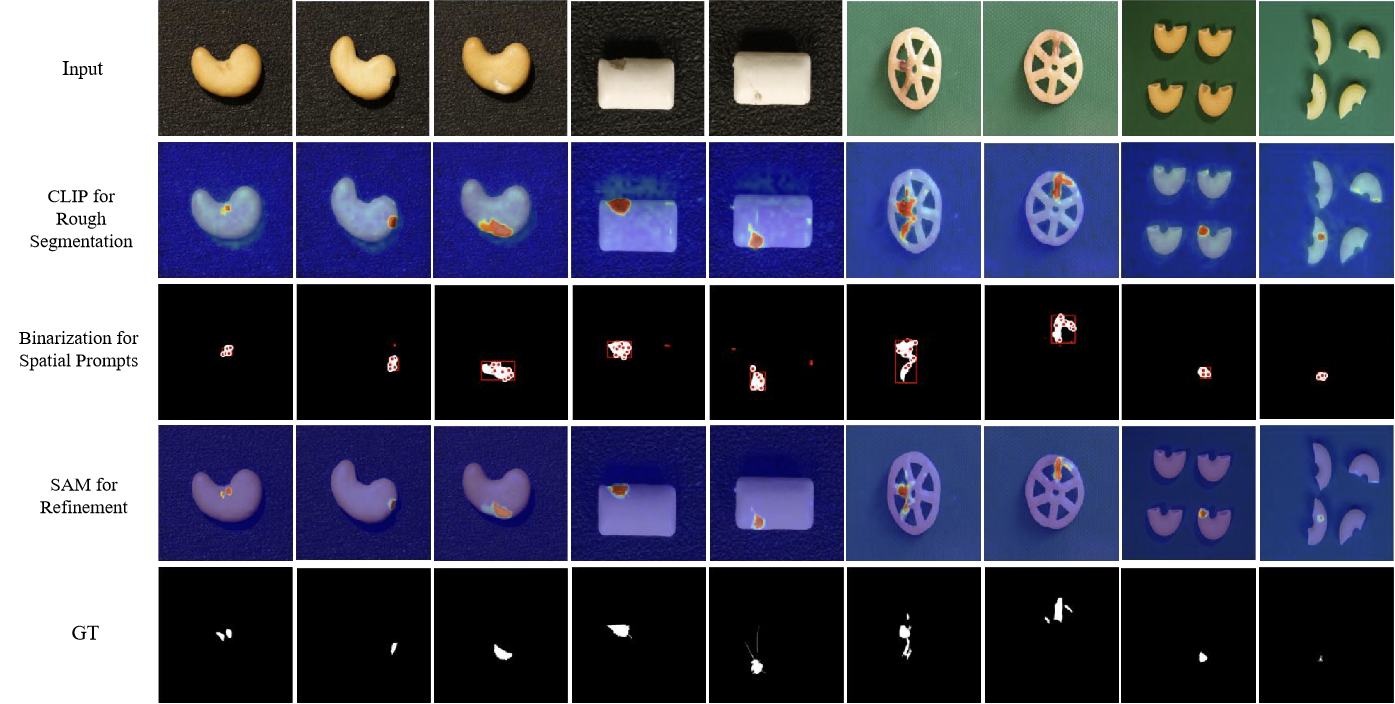
Figure 17: Visualization of different stages (the process of localization and rough segmentation by CLIP followed by result refinement through SAM) under the ClipSAM framework on the VisA dataset.

		MVTec-AD				VisA
Base model	Method	AUROC	$F_{1}$-max	AP	PRO	AUROC	$F_{1}$-max	AP	PRO
CLIP-based Approaches	WinCLIP	85.1	31.7	-	64.6	79.6	14.8	-	56.8
	APRIL-GAN	87.6	43.3	40.8	44.0	94.2	32.3	25.7	86.8
	AnoVL	90.6	36.5	-	77.8	91.4	17.4	-	75.0
	AnomalyCLIP	91.1	-	-	81.4	95.5	-	-	87.0
	SDP	88.7	35.3	28.5	79.1	84.1	16.0	9.6	63.4
	SDP+	91.2	41.9	39.4	85.6	94.8	26.5	20.3	85.3
SAM-based Approaches	SAA	67.7	23.8	15.2	31.9	83.7	12.8	5.5	41.9
	SAA+	73.2	37.8	28.8	42.8	74.0	27.1	22.4	36.8
CLIP & SAM	ClipSAM(Ours)	92.3	47.8	45.9	88.3	95.6	33.1	26.0	87.5

Table 5: Performance comparison of different kinds of ZSAS approaches on the MVTec-AD and VisA datasets. Evaluation metrics include AUROC, $F_{1}$-max, AP, and PRO. Bold indicates the best results.

The ClipSAM framework consists of two stages. In the first stage, CLIP is employed for localization and rough segmentation, while the second stage utilizes SAM for refining the results. During the process, we binarize the rough segmentation output of CLIP to generate spatial prompts as constraints in connected regions, namely points and boxes. We visualize each of these steps separately to qualitatively observe the output of each stage of the model.

As illustrated in Figure 15 and  16, with the assistance of the Unified Multi-scale Cross-modal Interaction (UMCI) module, CLIP achieves rough segmentation of abnormal regions. However, due to CLIP learning multi-modal semantics tailored for classification tasks, it has limitations in fine-grained segmentation tasks. This is typically manifested as CLIP correctly predicting only parts of a given real anomalous region. With the aid of SAM, it is possible to further refine the abnormal regions predicted by CLIP, obtaining abnormal masks that are closer to ground truth values. It is noteworthy that the binarization of results is based on a certain threshold, which usually does not result in a one-to-one correspondence between the red regions in the rough segmentation output and the connected regions in the binarized mask.

Additionally, as shown in Figure 17, due to the typically small size of anomaly categories in the ViSA dataset, the designed UMCI module has already assisted CLIP in achieving accurate anomaly segmentation. However, these results often exceed the ground truth values, as seen in the second column of the figure. SAM aids in further focusing on these small anomalous areas. After merging the masks generated by SAM with the rough segmentation results, a certain value suppression is applied to regions beyond the ground truth, which is advantageous when computing metrics.

Appendix F Comparing with more methods.

We additionally compared the model’s performance on zero-shot anomaly segmentation with two other works, AnoVL Deng et al. (2023) and AnomalyCLIP Zhou et al. (2023). AnoVL enhances the prompt templates with domain-specific textual designs such as ”industrial” and ”manufacturing.” AnomalyCLIP introduces the concept of prompt learning to the text encoder part of CLIP. As shown in the Table 5, our approach still achieves optimal performance on the zero-shot anomaly segmentation task. However, it is noteworthy that the design for text generality is an interesting approach for addressing zero-shot anomaly segmentation tasks. ClipSAM adopts the text strategy from WinCLIP Jeong et al. (2023) without further modifications, presenting a potential challenge for future exploration.

References

- Bergmann et al. [2019] Paul Bergmann, Michael Fauser, David Sattlegger, and Carsten Steger. Mvtec ad–a comprehensive real-world dataset for unsupervised anomaly detection. In Proceedings of the IEEE/CVF conference on computer vision and pattern recognition, pages 9592–9600, 2019.
- Bergmann et al. [2020] Paul Bergmann, Michael Fauser, David Sattlegger, and Carsten Steger. Uninformed students: Student-teacher anomaly detection with discriminative latent embeddings. In Proceedings of the IEEE/CVF conference on computer vision and pattern recognition, pages 4183–4192, 2020.
- Bergmann et al. [2022] Paul Bergmann, Kilian Batzner, Michael Fauser, David Sattlegger, and Carsten Steger. Beyond dents and scratches: Logical constraints in unsupervised anomaly detection and localization. International Journal of Computer Vision, 130(4):947–969, 2022.
- Božič et al. [2021] Jakob Božič, Domen Tabernik, and Danijel Skočaj. Mixed supervision for surface-defect detection: from weakly to fully supervised learning. Computers in Industry, 2021.
- Brown et al. [2020] Tom Brown, Benjamin Mann, Nick Ryder, Melanie Subbiah, Jared D Kaplan, Prafulla Dhariwal, Arvind Neelakantan, Pranav Shyam, Girish Sastry, Amanda Askell, et al. Language models are few-shot learners. Advances in neural information processing systems, 33:1877–1901, 2020.
- Cao et al. [2023] Yunkang Cao, Xiaohao Xu, Chen Sun, Yuqi Cheng, Zongwei Du, Liang Gao, and Weiming Shen. Segment any anomaly without training via hybrid prompt regularization. arXiv preprint arXiv:2305.10724, 2023.
- Chen et al. [2019] Ding-Jie Chen, Songhao Jia, Yi-Chen Lo, Hwann-Tzong Chen, and Tyng-Luh Liu. See-through-text grouping for referring image segmentation. In Proceedings of the IEEE/CVF International Conference on Computer Vision, pages 7454–7463, 2019.
- Chen et al. [2023a] Xuhai Chen, Yue Han, and Jiangning Zhang. A zero-/few-shot anomaly classification and segmentation method for cvpr 2023 vand workshop challenge tracks 1&2: 1st place on zero-shot ad and 4th place on few-shot ad. arXiv preprint arXiv:2305.17382, 2023.
- Chen et al. [2023b] Xuhai Chen, Jiangning Zhang, Guanzhong Tian, Haoyang He, Wuhao Zhang, Yabiao Wang, Chengjie Wang, Yunsheng Wu, and Yong Liu. Clip-ad: A language-guided staged dual-path model for zero-shot anomaly detection. arXiv preprint arXiv:2311.00453, 2023.
- Chen et al. [2023c] Yuxiao Chen, Jianbo Yuan, Yu Tian, Shijie Geng, Xinyu Li, Ding Zhou, Dimitris N Metaxas, and Hongxia Yang. Revisiting multimodal representation in contrastive learning: from patch and token embeddings to finite discrete tokens. In Proceedings of the IEEE/CVF Conference on Computer Vision and Pattern Recognition, pages 15095–15104, 2023.
- Cho et al. [2014] Kyunghyun Cho, Bart Van Merriënboer, Dzmitry Bahdanau, and Yoshua Bengio. On the properties of neural machine translation: Encoder-decoder approaches. arXiv preprint arXiv:1409.1259, 2014.
- Deng et al. [2023] Hanqiu Deng, Zhaoxiang Zhang, Jinan Bao, and Xingyu Li. Anovl: Adapting vision-language models for unified zero-shot anomaly localization. arXiv preprint arXiv:2308.15939, 2023.
- Devlin et al. [2018] Jacob Devlin, Ming-Wei Chang, Kenton Lee, and Kristina Toutanova. Bert: Pre-training of deep bidirectional transformers for language understanding. arXiv preprint arXiv:1810.04805, 2018.
- Ding et al. [2019] Xiaohan Ding, Yuchen Guo, Guiguang Ding, and Jungong Han. Acnet: Strengthening the kernel skeletons for powerful cnn via asymmetric convolution blocks. In Proceedings of the IEEE/CVF International Conference on Computer Vision (ICCV), October 2019.
- Feng et al. [2021] Guang Feng, Zhiwei Hu, Lihe Zhang, Jiayu Sun, and Huchuan Lu. Bidirectional relationship inferring network for referring image localization and segmentation. IEEE Transactions on Neural Networks and Learning Systems, 2021.
- Fomalont [1999] Ed B Fomalont. Image analysis. In Synthesis Imaging in Radio Astronomy II, volume 180, page 301, 1999.
- Gu et al. [2023] Zhaopeng Gu, Bingke Zhu, Guibo Zhu, Yingying Chen, Ming Tang, and Jinqiao Wang. Anomalygpt: Detecting industrial anomalies using large vision-language models. arXiv preprint arXiv:2308.15366, 2023.
- He et al. [2016] Kaiming He, Xiangyu Zhang, Shaoqing Ren, and Jian Sun. Deep residual learning for image recognition. In Proceedings of the IEEE conference on computer vision and pattern recognition, pages 770–778, 2016.
- Hou et al. [2020] Qibin Hou, Li Zhang, Ming-Ming Cheng, and Jiashi Feng. Strip pooling: Rethinking spatial pooling for scene parsing. In Proceedings of the IEEE/CVF Conference on Computer Vision and Pattern Recognition (CVPR), June 2020.
- Hu et al. [2016] Ronghang Hu, Marcus Rohrbach, and Trevor Darrell. Segmentation from natural language expressions. In Computer Vision–ECCV 2016: 14th European Conference, Amsterdam, The Netherlands, October 11–14, 2016, Proceedings, Part I 14, pages 108–124. Springer, 2016.
- Huang et al. [2019] Zilong Huang, Xinggang Wang, Lichao Huang, Chang Huang, Yunchao Wei, and Wenyu Liu. Ccnet: Criss-cross attention for semantic segmentation. In Proceedings of the IEEE/CVF International Conference on Computer Vision (ICCV), October 2019.
- Huang et al. [2020] Yibin Huang, Congying Qiu, and Kui Yuan. Surface defect saliency of magnetic tile. The Visual Computer, 36:85–96, 2020.
- Jeong et al. [2023] Jongheon Jeong, Yang Zou, Taewan Kim, Dongqing Zhang, Avinash Ravichandran, and Onkar Dabeer. Winclip: Zero-/few-shot anomaly classification and segmentation. In Proceedings of the IEEE/CVF Conference on Computer Vision and Pattern Recognition, pages 19606–19616, 2023.
- Jing et al. [2021] Ya Jing, Tao Kong, Wei Wang, Liang Wang, Lei Li, and Tieniu Tan. Locate then segment: A strong pipeline for referring image segmentation. In Proceedings of the IEEE/CVF Conference on Computer Vision and Pattern Recognition, pages 9858–9867, 2021.
- Khattak et al. [2023] Muhammad Uzair Khattak, Syed Talal Wasim, Muzammal Naseer, Salman Khan, Ming-Hsuan Yang, and Fahad Shahbaz Khan. Self-regulating prompts: Foundational model adaptation without forgetting. In Proceedings of the IEEE/CVF International Conference on Computer Vision, pages 15190–15200, 2023.
- Kirillov et al. [2023] Alexander Kirillov, Eric Mintun, Nikhila Ravi, Hanzi Mao, Chloe Rolland, Laura Gustafson, Tete Xiao, Spencer Whitehead, Alexander C. Berg, Wan-Yen Lo, Piotr Dollár, and Ross Girshick. Segment anything. arXiv:2304.02643, 2023.
- Lin et al. [2017] Tsung-Yi Lin, Priya Goyal, Ross Girshick, Kaiming He, and Piotr Dollár. Focal loss for dense object detection. In Proceedings of the IEEE international conference on computer vision, pages 2980–2988, 2017.
- Liu et al. [2023] Tongkun Liu, Bing Li, Xiao Du, Bingke Jiang, Xiao Jin, Liuyi Jin, and Zhuo Zhao. Component-aware anomaly detection framework for adjustable and logical industrial visual inspection. arXiv preprint arXiv:2305.08509, 2023.
- Milletari et al. [2016] Fausto Milletari, Nassir Navab, and Seyed-Ahmad Ahmadi. V-net: Fully convolutional neural networks for volumetric medical image segmentation. In 2016 fourth international conference on 3D vision (3DV), pages 565–571. Ieee, 2016.
- Mishra et al. [2021] Pankaj Mishra, Riccardo Verk, Daniele Fornasier, Claudio Piciarelli, and Gian Luca Foresti. Vt-adl: A vision transformer network for image anomaly detection and localization. In 2021 IEEE 30th International Symposium on Industrial Electronics (ISIE), pages 01–06. IEEE, 2021.
- Radford et al. [2021] Alec Radford, Jong Wook Kim, Chris Hallacy, Aditya Ramesh, Gabriel Goh, Sandhini Agarwal, Girish Sastry, Amanda Askell, Pamela Mishkin, Jack Clark, et al. Learning transferable visual models from natural language supervision. In International conference on machine learning, pages 8748–8763. PMLR, 2021.
- Rafiei et al. [2023] Mehdi Rafiei, Toby P Breckon, and Alexandros Iosifidis. On pixel-level performance assessment in anomaly detection. arXiv preprint arXiv:2310.16435, 2023.
- Vaswani et al. [2017] Ashish Vaswani, Noam Shazeer, Niki Parmar, Jakob Uszkoreit, Llion Jones, Aidan N Gomez, Łukasz Kaiser, and Illia Polosukhin. Attention is all you need. Advances in neural information processing systems, 30, 2017.
- Wang et al. [2022] Zhaoqing Wang, Yu Lu, Qiang Li, Xunqiang Tao, Yandong Guo, Mingming Gong, and Tongliang Liu. Cris: Clip-driven referring image segmentation. In Proceedings of the IEEE/CVF Conference on Computer Vision and Pattern Recognition (CVPR), pages 11686–11695, June 2022.
- Wang et al. [2023] Haoxiang Wang, Pavan Kumar Anasosalu Vasu, Fartash Faghri, Raviteja Vemulapalli, Mehrdad Farajtabar, Sachin Mehta, Mohammad Rastegari, Oncel Tuzel, and Hadi Pouransari. Sam-clip: Merging vision foundation models towards semantic and spatial understanding. arXiv preprint arXiv:2310.15308, 2023.
- Xu et al. [2023] Zunnan Xu, Zhihong Chen, Yong Zhang, Yibing Song, Xiang Wan, and Guanbin Li. Bridging vision and language encoders: Parameter-efficient tuning for referring image segmentation. In Proceedings of the IEEE/CVF International Conference on Computer Vision, pages 17503–17512, 2023.
- Yang and Gong [2024] Xiaobo Yang and Xiaojin Gong. Foundation model assisted weakly supervised semantic segmentation. In Proceedings of the IEEE/CVF Winter Conference on Applications of Computer Vision, pages 523–532, 2024.
- Yang et al. [2023] Minghui Yang, Peng Wu, and Hui Feng. Memseg: A semi-supervised method for image surface defect detection using differences and commonalities. Engineering Applications of Artificial Intelligence, 119:105835, 2023.
- Ye et al. [2022a] Peng Ye, Baopu Li, Tao Chen, Jiayuan Fan, Zhen Mei, Chen Lin, Chongyan Zuo, Qinghua Chi, and Wanli Ouyang. Efficient joint-dimensional search with solution space regularization for real-time semantic segmentation. International Journal of Computer Vision, 130(11):2674–2694, 2022.
- Ye et al. [2022b] Peng Ye, Baopu Li, Yikang Li, Tao Chen, Jiayuan Fan, and Wanli Ouyang. b-darts: Beta-decay regularization for differentiable architecture search. In Proceedings of the IEEE/CVF Conference on Computer Vision and Pattern Recognition, pages 10874–10883, 2022.
- Ye et al. [2022c] Peng Ye, Shengji Tang, Baopu Li, Tao Chen, and Wanli Ouyang. Stimulative training of residual networks: A social psychology perspective of loafing. Advances in Neural Information Processing Systems, 35:3596–3608, 2022.
- Yue et al. [2023] Wenxi Yue, Jing Zhang, Kun Hu, Qiuxia Wu, Zongyuan Ge, Yong Xia, Jiebo Luo, and Zhiyong Wang. Part to whole: Collaborative prompting for surgical instrument segmentation, 2023.
- Zhang et al. [2023a] Chaoning Zhang, Fachrina Dewi Puspitasari, Sheng Zheng, Chenghao Li, Yu Qiao, Taegoo Kang, Xinru Shan, Chenshuang Zhang, Caiyan Qin, Francois Rameau, et al. A survey on segment anything model (sam): Vision foundation model meets prompt engineering. arXiv preprint arXiv:2306.06211, 2023.
- Zhang et al. [2023b] Chunhui Zhang, Li Liu, Yawen Cui, Guanjie Huang, Weilin Lin, Yiqian Yang, and Yuehong Hu. A comprehensive survey on segment anything model for vision and beyond. arXiv preprint arXiv:2305.08196, 2023.
- Zhou et al. [2023] Qihang Zhou, Guansong Pang, Yu Tian, Shibo He, and Jiming Chen. Anomalyclip: Object-agnostic prompt learning for zero-shot anomaly detection. arXiv preprint arXiv:2310.18961, 2023.
- Zou et al. [2022] Yang Zou, Jongheon Jeong, Latha Pemula, Dongqing Zhang, and Onkar Dabeer. Spot-the-difference self-supervised pre-training for anomaly detection and segmentation. arXiv preprint arXiv:2207.14315, 2022.