EMITTANCE GROWTH OF DIFFERENT DISTRIBUTIONS

Abstract

The behavior of K-V, waterbag, parabolic, conical and Gaussian distributions in periodic quadrupole channels is studied by particle simulations. It is found that all these different distributions exhibit the known K-V instabilities. But the action of the K-V type modes becomes more and more damped in the order of the types of distributions quoted above. This damping is so strong for the Gaussian distribution that the emittance growth factor after a large number of periods is considerably lower than in the case of an equivalent K-V distribution.
In addition, the non K-V distributions experience in only one period of the channel a rapid initial emittance growth, which becomes very significant at high beam intensities. This growth is attributed to the homogenization of the space-charge density, resulting in a conversion of electric-field energy into transverse kinetic and potential energy. Two simple analytical formulae are derived to estimate the upper and lower boundary values for this effect and are compared with the results obtained from particle simulations.
 
Published in: Particle Accelerators 15, 47–65 (1984)

1 INTRODUCTION

Recent analytical and simulation studies by Hofmann, Laslett, Smith and Haber[1] show that the well-known K-V (Kapchinskij-Vladimirskij) distribution[2] is subject to instabilities in a periodic focusing channel. The region of these instabilities can be defined in terms of the phase advance of the particle oscillation per channel period without space charge, $\sigma_{0}$, and with space charge, $\sigma$. From these studies, the above authors concluded that one should impose the restriction $\sigma_{0}\leq 60^{\circ}$ to avoid the dangerous second-order (envelope) instabilities (occurring for $\sigma_{0}>90^{\circ}$) as well as the third-order mode ($\sigma_{0}>60^{\circ}$). In addition, they recommend to limit the beam intensity such that $\sigma\geq 24^{\circ}$ to avoid fourth- or higher-order instabilities. They point out, however, that this latter restriction may be too conservative in view of the fact that simulation studies for $\sigma_{0}\leq 60^{\circ}$ indicated that these higher-order modes saturate at low levels and that the rms emittance of a K-V distribution is not affected for $\sigma$ values as low as $6^{\circ}$.

In connection with the beam transport experiments at the University of Maryland[3] and at GSI,[4] we studied the behavior of K-V, waterbag, parabolic, conical and Gaussian distributions by particle simulation with the modified PARMILA code at GSI. Our goal was to determine whether more “realistic” non-stationary initial distributions are also affected by the instabilities found in a K-V beam (which represents the only stationary distribution in a periodic channel). Although each of these distributions is still artificially produced according to the appropriate phase-space density function, one expects that, with an increasing degree non-linearity, one comes closer and closer to a “real” beam. Of the different types considered, the truncated Gaussian distribution represents undoubtedly the closest approximation to a laboratory beam.

In a previous paper,[5] we reported the results of analytical and simulation work concerning envelope oscillations and (second-order) instabilities of mismatchedbeams. The particle simulation studies were restricted to K-V and Gaussian distributions and showed that, for the cases considered ($\sigma_{0}>90^{\circ}$), the effect of instabilities on an initial Gaussian distribution is even worse than for a K-V beam. These findings support the results of Ref. 1 that the region $\sigma_{0}>90^{\circ}$ must be avoided in the design and operation of transport channels for intense beams.

In the present paper we report the results of systematic studies with different initial particle distributions at values of $\sigma_{0}=90^{\circ}$ and $\sigma_{0}=60^{\circ}$. Of particular interest in the $\sigma_{0}=90^{\circ}$ case was the third-order instability. In contrast to our results on the envelope modes, we found that the Gaussian distribution remains almost unaffected by this mode. At the same time we discovered that the non-K-V distributions considered experience in the first period of the transport channel a rapid emittance growth which occurs even in regions where no instabilities are predicted and which increases approximately proportional to $\sigma^{-1}$. It will be shown that the emittance growth can be attributed to an internal redistribution of the particles toward a more uniform density profile, whereby field energy is converted into transverse kinetic energy.

2 PROPERTIES OF DIFFERENT PARTICLE DISTRIBUTIONS
FOR CONTINUOUS BEAMS

2.1 General Formulae

Two particle distributions are identical, if all their moments are the same. To allow a comparison of the results obtained with different distribution functions carrying the same current, we use the concept of equivalent beams introduced by Lapostolle[6] and Sacherer,[7] i.e., beams having the same first and second moments. Since we are dealing with continuous beams rather than bunched beams, the particle distributions occupy only a $4$-dimensional transverse phase space volume, usually approximated by a hyperellipsoid. For the sake of simplicity,this hyperellipsoid is transformed into a hypersphere, i.e., the particle density $f(r)$ only depends on the radial distance $r$; hence one has constant particle density on any hypersphere in the phase space

$$f(r={\rm const.})={\rm const.},\quad r^{2}=x^{2}+y^{2}+{x^{\prime}}^{2}+{y^{\prime}}^{2}.$$

For five different types of particle distributions, we have evaluated

• the ratio of the marginal emittance to the rms emittance,

• the particle (charge) density $g(x,y)$ in real space,

• the electric fields $E(r)$ inside the beam,

• the field energy $U$ associated with the charge distribution.

A given distribution function $f(r)$ is called normalized if

$$\int_{0}^{a}f(r)\,dV=1,$$

where $dV=d\Omega_{n}r^{n-1}dr$ denotes the volume element of the $n$-dimensional phase space in spherical coordinates, and $a$ the maximum value of $r$. In our case of a continuous beam, we have $n=4$. If we assume the beam to be centered, the first moments are zero and the second moments are given by[8]

$$\langle r^{2}\rangle=\frac{1}{n}\int_{0}^{a}r^{2}f(r)\,dV\bigg{/}\int_{0}^{a}f(r)\,dV.$$

Since the particle density only depends on $r$, the integrals can be simplified:

$$\langle r^{2}\rangle=\frac{1}{n}\int_{0}^{a}f(r)\,r^{n+1}\,dr\bigg{/}\int_{0}^{a}f(r)\,r^{n-1}\,dr.$$

The rms emittance of a distribution in the $x,x^{\prime}$-plane is defined as[6]

$$\varepsilon_{\rm rms}=4\cdot{\left[\langle x^{2}\rangle\langle{x^{\prime}}^{2}\rangle-{\langle xx^{\prime}\rangle}^{2}\right]}^{1/2}.$$

If the emittance ellipse is upright, one has $\langle xx^{\prime}\rangle=0$ and therefore

$$\varepsilon_{\rm rms}=\langle\varepsilon\rangle=4\cdot{\left[\langle x^{2}\rangle\langle{x^{\prime}}^{2}\rangle\right]}^{1/2}.$$

The factor $4$ is chosen so that the rms emittance of a K-V distribution is equal to the area $A$ divided by $\pi$ of the minimum circumscribing phase-space ellipse that encloses all particles. This number $A/\pi$ is usually called the maximum emittance $\varepsilon_{\rm max}$ of a distribution. The ratio $\varepsilon_{\rm max}/\varepsilon_{\rm rms}$ is then given by

$$\varepsilon_{\rm max}/\varepsilon_{\rm rms}=a^{2}/4\langle r^{2}\rangle={\textstyle\frac{1}{4}}na^{2}\cdot\int_{0}^{a}f(r)\,r^{n-1}\,dr\bigg{/}\int_{0}^{a}f(r)\,r^{n+1}\,dr.$$

The density in real space $g(x,y)$ is obtained by integration over the coordinates $x^{\prime}$ and $y^{\prime}$. In our case of a constant particle density on any hypersphere in the $4$-dimensional transverse phase space, one obtains with the substitution ${r^{\prime}}^{2}={x^{\prime}}^{2}+{y^{\prime}}^{2}$

$$g(x,y)=2\pi\cdot\int_{0}^{\sqrt{a^{2}-x^{2}-y^{2}}}f\big{(}x^{2}+y^{2}+{r^{\prime}}^{2}\big{)}\,r^{\prime}dr^{\prime}.$$

The electric field $E_{i}(r)$ inside the beam is obtained from Poisson’s equation

$$\frac{1}{r}\cdot\frac{d}{dr}\big{(}r\cdot\Phi^{\prime}(r)\big{)} = -q\cdot g(r),\quad q=I/\epsilon_{0}c\beta$$

$$E_{i}(r) = \frac{q}{r}\int_{0}^{r}g(\rho)\,\rho\,d\rho,$$

whereas the field in the region between beam and wall follows from Laplace’s equation. With $E_{i}(a)=E_{o}(a)$ one obtains for $r\geq a$

$$E_{o}(r)=\frac{q}{r}\int_{0}^{a}g(\rho)\,\rho\,d\rho=q/2\pi r.$$

The electric field energy $U$ of such a special charge distribution is finally given by

$$U=\pi\epsilon_{0}\cdot\left(\int_{0}^{a}{E_{i}}^{2}\,r\,dr+\int_{a}^{R}{E_{o}}^{2}\,r\,dr\right),$$

where $R$ denotes the wall radius.

Table 2.1 gives the definitions of the five particle distribution functions that we used in our work and their appropriate quantities quoted here.

2.2 Differences of The Field Energy Associated with Different Distribution Functions

As can be seen in Table 2.1, each charge distribution function is associated with a specific electric field energy. The minimum field energy of a charge distribution applies to the homogeneous charge density in real space associated with a K-V distribution in phase space.

Assuming that each distribution has the same second moments (or rms emittance), as stated earlier, one finds that the field energy $U$ increases from the K-V to the Gauss distribution. One can write the difference between a particular distribution and the K-V distribution in the form

$$\Delta U=U-U_{\rm KV}=f\cdot u_{0},$$

where

$$u_{0}=I^{2}/4\pi\epsilon_{0}c^{2}\beta^{2}=10^{-7}\cdot(I/\beta)^{2}\quad\left[\,{\rm joules/meter}\,\right].$$

The factors $f$ for the field-energy difference between each distribution and the equivalent K-V beam are listed in Table 1. As an example, one finds for the additional field energy stored in a Gaussian distribution compared to an equivalent K-V beam

$$\Delta U=U_{\rm GA}-U_{\rm KV}=u_{0}\cdot({\textstyle\frac{1}{2}}C-{\textstyle\frac{1}{4}})=u_{0}f,$$

with

$$f={\textstyle\frac{1}{2}}C-{\textstyle\frac{1}{4}}\simeq 0.0386,$$

wherein $C\simeq 0.5772$ denotes Euler’s constant.

TABLE 1: $f$-Factors for the transition of different Charge-Distribution Functions

fromto	KV	WB	PA	CO
from
WB	0.00560	0	—	—
PA	0.01176	0.00616	0	—
CO	0.01408	0.00848	0.00232	0
GA	0.03861	0.03301	0.02685	0.02452

As will be explained in the next section, we surmise that this additional field energy is converted into particle kinetic and potential energy (and hence emittance growth) as the distribution tends to become more homogeneous. The average energy per particle of charge state $\zeta$ available for this transformation is

$$\Delta E=30fI\zeta/\beta=fu_{0}/N\quad\left[\,{\rm eV}\,\right],$$

where $N=I/\zeta e_{0}\beta c$ is the number of particles per unit length.

2.3 Emittance Growth Due to a Change of the Particle Distribution

Since the above defined non-K-V distributions are not stationary, they undergo a complete change during the transformation through a beam-transport line, leading to a more homogeneous charge distribution in real space as shown in Fig. 1 for different initial distributions transformed through one period of the GSI quadrupole channel, whose parameters are defined in Ref. 5. This process of a reorganization of the particle phase-space distribution toward a more self-consistent, i.e., stationary, one yields an increase of the quantities $\langle r^{2}\rangle$ and $\langle{r^{\prime}}^{2}\rangle$, hence an increase of the rms emittance of the beam, resulting from the transformation of internal field energy associated with the initial charge distribution to additional transverse kinetic and potential energy of the beam in the focusing channel.

$(a)\,\,\,\sigma\to\sigma_{0}$

In order to obtain an analytical estimate of the emittance growth for low intensities, an rms-matched non-K-V distribution that changes its charge density in real space towards a homogeneous one is treated as an equivalent K-V distribution that becomes “heated up”. An increase of the total energy of a particle will the result in an increase of both the mean kinetic energy (proportional to $\langle{x^{\prime}}^{2}\rangle$), and the mean potential energy (proportional to $\langle x^{2}\rangle$). The total energy $E_{\rm tot}$ of a single particle in that harmonic-oscillator potential may be expressed in terms of the tune shift $\sigma$, the length of one focusing period $S$, and transverse rms emittance $\langle\varepsilon\rangle$ as

$$E_{\rm tot}={\textstyle\frac{1}{4}}\gamma m_{0}c^{2}\beta^{2}\sigma\langle\varepsilon\rangle/S.$$

Here we assume that the motion in the longitudinal direction can be relativistic, (hence $\gamma m_{0}$ for the mass) while the transverse motion is non-relativistic. The mean energy gain per unit charge due to a homogenization of the charge distribution as evaluated in the previous section is for an arbitrary transverse spatial plane

$$\Delta E={\textstyle\frac{1}{2}}fIe_{0}/4\pi\epsilon_{0}c\beta\gamma^{2},$$

where the factor ${\textstyle\frac{1}{2}}$ results from the reduction to one degree of freedom. If the superscript ⁺ denotes the appropriate quantities after the homogenization of the charge distribution, we obtain for the total energies

$${\textstyle\frac{1}{4}}\gamma m_{0}c^{2}\beta^{2}\sigma\langle\varepsilon\rangle/S+{\textstyle\frac{1}{2}}fIe_{0}/4\pi\epsilon_{0}c\beta\gamma^{2}={\textstyle\frac{1}{4}}\gamma m_{0}c^{2}\beta^{2}\sigma\langle\varepsilon\rangle^{+}/S.$$

Thus

$$\sigma\langle\varepsilon\rangle+2fIS/I_{0}\beta^{3}\gamma^{3}=\sigma^{+}\langle\varepsilon\rangle^{+},$$

where $I_{0}=4\pi\epsilon_{0}m_{0}c^{3}/e_{0}$ is the limiting current as defined in Ref. 5. Since $\sigma$ does not remain constant during reorganization of the particle distribution but increases to $\sigma^{+}$, we have to express $\sigma^{+}$ in terms of $\langle\varepsilon\rangle^{+}$. According to the smooth-approximation theory of Ref. 9, this means

$$\sigma^{+}=\sigma_{0}\left(\sqrt{1+{u^{+}}^{2}}-u^{+}\right),\quad u^{+}=IS/I_{0}\beta^{3}\gamma^{3}\sigma_{0}\langle\varepsilon\rangle^{+}.$$

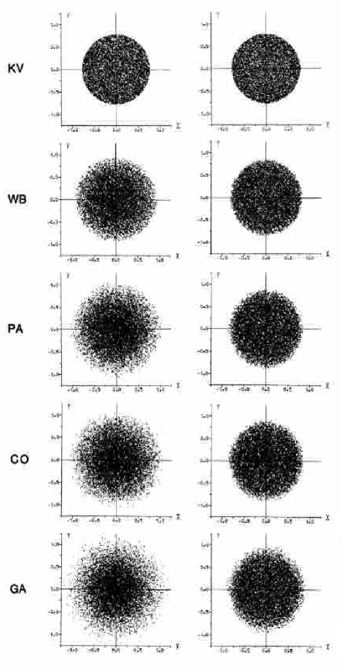
FIGURE 1: Real-space $(x,y)$ projections of K-V, waterbag, parabolic, conical and Gaussian distributions before and after the first cell of the GSI FODO channel at $\sigma_{0}=60^{\circ}$, $\sigma=15^{\circ}$.

Solving for the ratio $\langle\varepsilon\rangle^{+}/\langle\varepsilon\rangle$, one obtains after some algebraic transformations

$$\frac{\langle\varepsilon\rangle^{+}}{\langle\varepsilon\rangle}=\sqrt{\left(\frac{\sigma}{\sigma_{0}}+2uf\right)\left(\frac{\sigma}{\sigma_{0}}+2uf+2u\right)}$$

with $u$ as defined above but now pertaining to the initial rms emittance $\langle\varepsilon\rangle$. $u$ can easily be expressed in terms of $\sigma_{0}$ and $\sigma$ as

$$2u=\frac{\sigma_{0}}{\sigma}-\frac{\sigma}{\sigma_{0}}.$$

The formula for the relative growth of the transverse rms emittance then reduces to

$$\frac{\langle\varepsilon\rangle^{+}}{\langle\varepsilon\rangle}=\sqrt{\left[1+f\cdot\left(\frac{{\sigma_{0}}^{2}}{\sigma^{2}}-1\right)\right]\left[1+f\cdot\left(1-\frac{\sigma^{2}}{{\sigma_{0}}^{2}}\right)\right]}.$$

$(b)\,\,\,\sigma\to 0$

For non-K-V distributions, the effective potential well is no longer harmonic. Especially for high intensities, the effective potential becomes more and more “flat” in the central region of the beam, and has a sharp increase at the beam boundary. This type of potential function may be called a “reflecting-wall potential” since the particles are moving nearly force-free inside the beam and are reflected at its boundary. The additional internal electric field energy is then only transformed into transverse kinetic energy, hence resulting in an increase of $\langle{r^{\prime}}^{2}\rangle$. In order to obtain a formula to estimate these cases, we use again the model of a harmonic oscillator. But now only the mean kinetic energy of a particle is increased, whereas its mean potential energy is assumed to remain constant. Since the mean transverse kinetic energy of one particle is given by

$$E_{k}={\textstyle\frac{1}{2}}\gamma m_{0}c^{2}\beta^{2}\langle{x^{\prime}}^{2}\rangle,$$

the energy equation may then be written as

$${\textstyle\frac{1}{2}}\gamma m_{0}c^{2}\beta^{2}\langle{x^{\prime}}^{2}\rangle+{\textstyle\frac{1}{2}}fIe_{0}/4\pi\epsilon_{0}c\beta\gamma^{2} = {\textstyle\frac{1}{2}}\gamma m_{0}c^{2}\beta^{2}\langle{x^{\prime}}^{2}\rangle^{+}$$

$$\langle{x^{\prime}}^{2}\rangle+fI/I_{0}\beta^{3}\gamma^{3} = \langle{x^{\prime}}^{2}\rangle^{+}.$$

At a position where the emittance ellipse is upright ($\langle xx^{\prime}\rangle=0$), we obtain

$$\big{(}\langle\varepsilon\rangle^{+}\big{)}^{2}=\langle\varepsilon\rangle^{2}+16fI\langle x^{2}\rangle/I_{0}\beta^{3}\gamma^{3}.$$

With the relation

$$\langle x^{2}\rangle={\textstyle\frac{1}{4}}\langle\varepsilon\rangle S/\sigma,$$

which is valid a particle moving in a harmonic oscillator potential, this finally leads to

$$\frac{\langle\varepsilon\rangle^{+}}{\langle\varepsilon\rangle}=\sqrt{1+2f\cdot\left(\frac{{\sigma_{0}}^{2}}{\sigma^{2}}-1\right)}.$$

3 SIMULATION STUDIES

3.1 Third-Order Instability with Equivalent Beams of Different Particle Distributions

The space-charge potential of a K-V distribution is a quadratic function of the spatial coordinates leading to linear forces. As has been shown previously, the K-V distribution is unstable against perturbations of this potential distributions in some specific regions depending on the external forces (defined by the phase advance $\sigma_{0}$) and the beam parameters (defined by $\sigma$). The type of perturbation can be classified by the order of additional potential terms. For example, a potential proportional to $xy^{2}$ called a “third-order” perturbation potential. For $\sigma_{0}=90^{\circ}$, the K-V distribution is unstable against this type of perturbation in the region $38^{\circ}\leq\sigma\leq 60^{\circ}$. To evaluate whether and how this instability affects the non-K-V distributions defined above, we performed simulation studies for $\sigma_{0}=90^{\circ}$ and $\sigma=41^{\circ}$, hence near the maximum growth rate for third-order mode in a K-V beam. All computer runs discussed in this paper were made with the parameters of the GSI quadrupole channel (see Ref. 5).

Figure 2 shows the evolution of an initial K-V distribution. The specific instability can easily be recognized by the three “arms” growing out of the initial elliptic particle distribution. After about $50$ periods the transverse rms emittance has grown to a factor of $2.2$, remaining nearly constant during the following sections.

Figure 3 shows the transformation of an equivalent initial waterbag distribution under the same conditions ($\sigma_{0}=90^{\circ}$, $\sigma=41^{\circ}$). The resulting type of distortion is obviously the same, yet the growing of “arms” is less pronounced in that case. The rms emittance growth factor of $2.2$ after $100$ periods shows no essential difference to that of the K-V distribution.

Figure 4 shows the evolution of an initial parabolic transverse particle density distribution , where the patterns of the emittance plots are similar to that of the waterbag distribution, yielding a saturated transverse rms emittance growth of $2.2$ after $100$ periods.

The evolution of the conical distribution, plotted in Fig. 5, shows a less pronounced third-order instability mode compared to the previous types of distributions. The growth factor of the rms emittance is lower than in these cases reaching a value of $\simeq 1.8$ after $100$ periods.

The last density distribution investigated here is the Gaussian distribution truncated at $a=4\sqrt{\langle x^{2}\rangle}$, whose evolution is shown in Fig. 6. A nearly constant slight increase in rms emittance is obtained and no saturation of that growth can be recognized after $100$ periods, where the growth factor of the rms emittance amounts to only $\simeq 1.2$.

Period      ​0                   20                  40                  60                  ​100

FIGURE 2: Transformation of an initial K-V distribution through the GSI FODO channel at $\sigma_{0}=90^{\circ},\sigma=41^{\circ}$. (The $x,x^{\prime}$ and $y,y^{\prime}$ phase-space projections are represented in normal form.)

Period      ​0                   20                  40                  60                  ​100

FIGURE 3: Transformation of an initial waterbag distribution through the GSI FODO channel at $\sigma_{0}=90^{\circ},\sigma=41^{\circ}$. (The $x,x^{\prime}$ and $y,y^{\prime}$ phase-space projections are represented in normal form.)

Period      ​0                   20                  40                  60                  ​100

FIGURE 4: Transformation of an initial parabolic distribution through the GSI FODO channel at $\sigma_{0}=90^{\circ},\sigma=41^{\circ}$. (The $x,x^{\prime}$ and $y,y^{\prime}$ phase-space projections are represented in normal form.)

Period      ​0                   20                  40                  60                  ​100

FIGURE 5: Transformation of an initial conical distribution through the GSI FODO channel at $\sigma_{0}=90^{\circ},\sigma=41^{\circ}$. (The $x,x^{\prime}$ and $y,y^{\prime}$ phase-space projections are represented in normal form.)

Period      ​0                   20                  40                  60                  ​100

FIGURE 6: Transformation of an initial Gaussian distribution through the GSI FODO channel at $\sigma_{0}=90^{\circ},\sigma=41^{\circ}$. (The $x,x^{\prime}$ and $y,y^{\prime}$ phase-space projections are represented in normal form.)

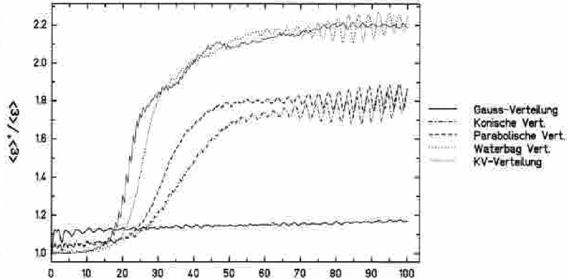
Cell Number

FIGURE 7: Emittance growth factors versus the number of cells obtained from particle simulations for initial K-V, waterbag, parabolic, conical, and Gaussian distributions at $\sigma_{0}=90^{\circ}$, $\sigma=41^{\circ}$.

Figure 7 shows the increase of the transverse rms emittance versus the number of cells for our five types of distribution functions. The initial offset of the non-K-V distributions is due to the homogenization effect of the particle density in real space mentioned in the previous chapter. According to the emittance-growth formulae derived in Section 2.3, with which the lower and the upper limits of this effect can be estimated, this leads to an initial growth of $1.3\%$ to $2.1\%$ for the waterbag, $2.7\%$ – $4.4\%$ for the parabolic, $3.2\%$ – $5.2\%$ for the conical, and $8.7\%$ – $13.8\%$ for the Gaussian distribution. This agrees with the simulation results plotted in Fig. 7, since the obtained initial emittance growth factors lie between these values.

The final saturation of the emittance growth leads to the value of $\simeq 2.3$, except for the conical and Gaussian distributions, which continue to increase at lower levels. The slope of the emittance growth decreases from the K-V towards the Gaussian distribution, and therefore the number of cells, where a saturation can be observed, if there is any, increases. This is due to the increasing spread in the individual particle tunes $\sigma$, which minimizes the effect of the resonance. This effect remains to be investigated.

For comparison, Fig. 8 shows the increase of the rms emittance versus the cell number of $\sigma_{0}=60^{\circ}$, $\sigma=25^{\circ}$. No structure resonance is present under these conditions in agreement with Ref. 1. So the rms emittance growth factors obtained from numerical simulations are only due to the initial homogenization of the charge density, amounting to $\simeq 1.7\%$ for the waterbag, $\simeq 4.0\%$ for the parabolic, $\simeq 5.0\%$ for the conical, and $12.5\%$ for the Gaussian distribution. These factors lie between the appropriate emittance growth factors evaluated with our formulae (indicated by the horizontal lines in Fig. 8).

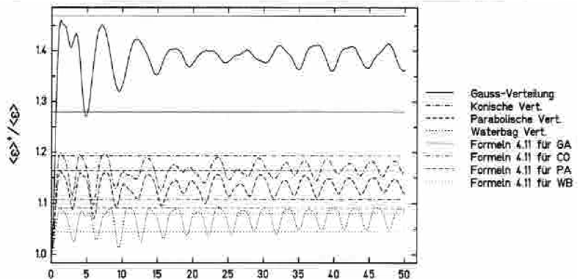
Cell Number

FIGURE 8: Emittance growth factors versus the number of cells obtained from particle simulations for initial K-V, waterbag, parabolic, conical, and Gaussian distributions at $\sigma_{0}=60^{\circ}$, $\sigma=25^{\circ}$.

3.2 K-V and Gaussian Distributions at Increasing Intensities

In view of the fact that a Gaussian distribution comes perhaps closest to a real beam, we investigated its behavior over a wide parameter range of decreasing $\sigma$ values (i.e., increasing intensity) and compared it with a K-V distribution. We made a large number of simulation runs for the two distributions at fixed values of $\sigma_{0}=90^{\circ}$ and $\sigma_{0}=60^{\circ}$ using as before the geometry of the GSI channel.

$(a)\,\,\,\sigma_{0}=90^{\circ}$

Figure 9 shows the rms emittance growth after $100$ cells for a K-V and a Gaussian distortion at $\sigma_{0}=90^{\circ}$ and various values of $\sigma$. As can be seen, the two types distribution functions behave quite differently:

• The K-V distribution shows the expected emittance growth due to a third-order instability in the region $60^{\circ}\geq\sigma\geq 38^{\circ}$. The sharp decrease of the emittance growth at $\sigma\simeq 38^{\circ}$ indicates that the third-order instability is no longer present. As $\sigma$ decreases, i.e., at higher intensities, the fourth- and higher-order modes take effect in the region $\sigma<37^{\circ}$.

• The Gaussian distribution shows a monotonic increase in the emittance growth factors as $\sigma$ decreases. One part of the emittance growth can be attributed to the homogenization effect discussed in Section $2.3$, since a sharp rise in rms emittance occurs within the first cell. The emittance growth as calculated from our formulae are indicated by the dashed line for the lower boundary value (Formula $1$) and by the dotted line for upper one (Formula $2$). It is seen that the actual emittance growth is considerably larger than the formulae predict. This difference suggests that the action of the resonances in the region $\sigma<60^{\circ}$ is still present.

$(b)\,\,\,\sigma_{0}=60^{\circ}$

Figure 10 shows the rms emittance growth after $50$ cells for a K-V and a Gaussian distribution at $\sigma_{0}=60^{\circ}$. For the K-V distribution, no emittance growth occurs above $\sigma=10^{\circ}$. Below that value, a small growth is obtained, which is due to a fourth-order instability mode.

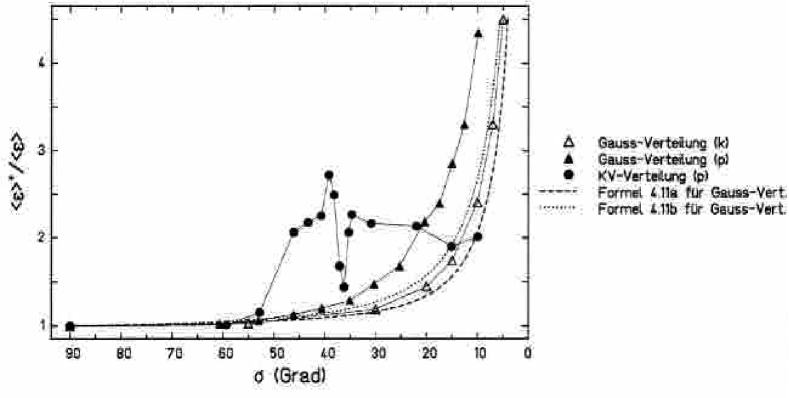
FIGURE 9: Emittance growth factors versus $\sigma$ after $100$ cells for initial K-V and Gaussian distributions at $\sigma_{0}=90^{\circ}$.

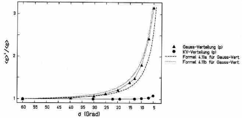
FIGURE 10: Emittance growth factors versus $\sigma$ after $50$ cells for initial K-V and Gaussian distributions at $\sigma_{0}=60^{\circ}$.

The emittance growth factors for Gaussian distribution obtained from particle simulations lie exactly between those calculated from the emittance growth formulae derived above, as the comparison of dotted analytical curves with the simulation results indicate. This suggests that the Gaussian distribution, like the K-V distribution is also stable with respect to fourth- and higher-order modes under these conditions, and that the emittance growth can be explained in terms of the homogenization effect. This explanation is confirmed by the fact, that in all simulation runs at values of $\sigma$ greater than $10^{\circ}$ no further emittance growth is observed after the initial change of the charge distribution in the first period of the channel.

4 CONCLUSIONS

The K-V distribution has been investigated by many authors, It has been found[1], that it shows a series of instabilities due to structure resonances in the case of a periodic transport system. A structure resonance of the $n$th order can be avoided, if $\sigma_{0}\leq 180^{\circ}/n$. These results have been confirmed by our simulation studies. The K-V distribution shows the typical third- and higher-order modes for $\sigma_{0}=90^{\circ}$. and the fourth- and higher-order instabilities for $\sigma_{0}=60^{\circ}$, leading in both cases to a growth of the rms emittance. The simulation studies have been extended to four non-K-V distributions: waterbag, parabolic, conical and Gaussian. Two types of additional effects have been found:

1. A damping of the structure resonances occurs, leading to a smaller slope in emittance growth. The action of the damping increases from the waterbag, parabolic, conical toward the Gaussian distribution.

2. A homogenization of the particle density in real space takes place within the first cell. This leads to an initial growth of the rms emittance due to transformation of field energy into kinetic and potential beam energy.

The effects of third- and higher-order instabilities are seen in the simulations of the non-K-V distribution, yet the typical patterns (a specific number of arms growing out of two dimensional $x,x^{\prime}$- and $y,y^{\prime}$-phase space projections) become more and more smoothed out. This effect increases from the waterbag towards the Gaussian distribution, where these patterns are no longer recognized.

The amount of the initial growth depends on the type of the initial distribution and also increases from the waterbag over the parabolic and conical towards the Gaussian distribution. For each distribution we calculated a factor $f$, which defines the difference between the field energy of the distribution and that of a K-V beam. Assuming first that this difference is transformed into kinetic and potential energy and secondly into kinetic energy only via homogenization of the charge density in real space, one obtains the estimate for the initial emittance growth

$$\sqrt{\left[1+f\cdot\left(\frac{{\sigma_{0}}^{2}}{\sigma^{2}}-1\right)\right]\left[1+f\cdot\left(1-\frac{\sigma^{2}}{{\sigma_{0}}^{2}}\right)\right]}<\frac{\langle\varepsilon\rangle^{+}}{\langle\varepsilon\rangle}<\sqrt{1+2f\cdot\left(\frac{{\sigma_{0}}^{2}}{\sigma^{2}}-1\right)}.$$

The results obtained with these formulae have been found in good agreement with those obtained by the simulation studies for $\sigma_{0}=60^{\circ}$ where no K-V instabilities are observed and where the “homogenization” is the only source of emittance growth. In the case of $\sigma_{0}=90^{\circ}$, the emittance growth factors are greater due to the additional action of structure resonances. Nevertheless it has been shown that the types of not self-consistent particle distributions treated in this paper show a specific increase of the rms emittance due to the internal matching of the charges to the linear external forces, even if they are perfectly rms-matched.

REFERENCES

- 1. I. Hofmann, L. J. Laslett, L. Smith, and I. Haber, Particle Accelerators, 13, 145 (1983).
- 2. I. M. Kapchinskij and V. V. Vladimirskij, Proc. Int. Conf. on High Energy Accelerators, CERN, Geneva, 1959, p. 274.
- 3. J. D. Lawson, E. Chojnacki, P. Loschialpo, W. Namkung, C. R. Prior, T. C. Randle, D. Reading, and M. Reiser, IEEE Trans. Nucl. Sci., 30, 2537 (1983).
- 4. J. Klabunde, M. Reiser, A. Schönlein, P. Spädtke, and J. Struckmeier, IEEE Trans. Nucl. Sci., 30, 2543 (1983).
- 5. J. Struckmeier and M. Reiser, “Theoretical Studies of Envelope Oscillations and Instabilities of Mismatched Intense Charged Particle Beams in Periodic Focusing Channels”, Particle Accelerators, 14, 227 (1984).
- 6. P. M. Lapostolle, IEEE Trans. Nucl. Sci., 18, 1101 (1971).
- 7. F. J. Sacherer, IEEE Trans. Nucl. Sci., 18, 1105 (1971).
- 8. B. Bru and M. Weiss, “Some Useful Formulae Concerning RMS-Values of Various Density Distributions”, CERN/MPS/LIN 74-1, Appendix I (1974).
- 9. M. Reiser, Particle Accelerators, 8, 167 (1978).