Fast Implicit Neural Representation Image Codec in Resource-limited Devices

Abstract.

Displaying high-quality images on edge devices, such as augmented reality devices, is essential for enhancing the user experience. However, these devices often face power consumption and computing resource limitations, making it challenging to apply many deep learning-based image compression algorithms in this field. Implicit Neural Representation (INR) for image compression is an emerging technology that offers two key benefits compared to cutting-edge autoencoder models: low computational complexity and parameter-free decoding. It also outperforms many traditional and early neural compression methods in terms of quality. In this study, we introduce a new Mixed Autoregressive Model (MARM) to significantly reduce the decoding time for the current INR codec, along with a new synthesis network to enhance reconstruction quality. MARM includes our proposed Autoregressive Upsampler (ARU) blocks, which are highly computationally efficient, and ARM from previous work to balance decoding time and reconstruction quality. We also propose enhancing ARU’s performance using a checkerboard two-stage decoding strategy. Moreover, the ratio of different modules can be adjusted to maintain a balance between quality and speed. Comprehensive experiments demonstrate that our method significantly improves computational efficiency while preserving image quality. With different parameter settings, our method can outperform popular AE-based codecs in constrained environments in terms of both quality and decoding time, or achieve state-of-the-art reconstruction quality compared to other INR codecs.

1. Introduction

Recent years have seen dramatic advancements in deep learning-based lossy image compression (Ballé et al., 2016, 2018; Minnen et al., 2018a; He et al., 2022). These advancements have led to significant progress, outperforming many traditional image codecs such as JPEG (Wallace, 1992) and BPG (Bellard, 2018) across common metrics like PSNR and MS-SSIM (Wang et al., 2003). Joint backward-and-forward adaptive entropy modeling is a crucial technique in these models, utilizing side information in forward adaptation and predictions from the causal context of each symbol in backward adaptation (Minnen et al., 2018b; Minnen and Singh, 2020; Cheng et al., 2020). In addition to neural image codecs based on autoencoders (AE), there has been an emergence of implicit neural representation (INR) in 3D applications, utilizing neural network weights to represent information, and this has spurred exploration into similar technologies in image compression. Dupont et al. (Dupont et al., 2021a) proposed using 2D coordinates as the input for the MLP and directly outputting the RGB value of the corresponding pixel. Expanding on this, Ladune et al. (Ladune et al., 2023) introduced COOL-CHIC, which utilizes trainable latent variables as the input for the MLP.

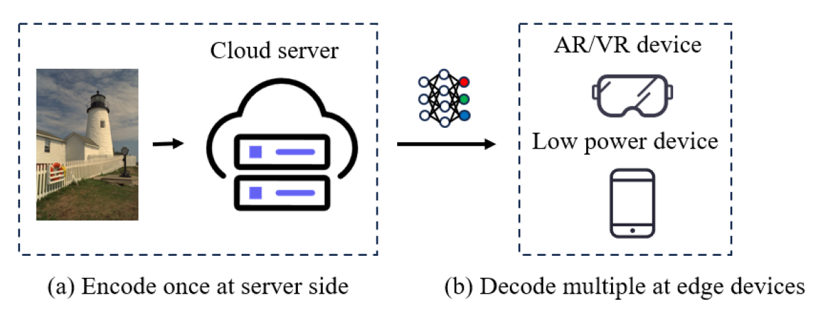
Figure 1. Asymmetric compression and decompression framework of the INR codec.

Although AE-based methods achieve better rate-distortion performance, INR-based methods offer several advantages. In the context of an asymmetric compression system, as shown in Fig. 1, edge devices often face power consumption or computing resource limitations that make it impractical to deploy AE-based methods. INR provides a low-complexity decoding method, which is essential for AR/VR devices and low-power devices such as smartphones or AR glasses. A single encoded bit stream can be decoded on many different devices to mitigate the heavy resource consumption during the encoding process completed at the server side. According to Leguay et al. (2023), INR-based methods achieve a similar BD-rate as HEVC and nearly two orders of magnitude less MACs (Multiplication-Accumulation) compared with AE-based methods. Moreover, unlike AE-based models, the decompression process of the INR codec does not require model parameters other than the transmitted part, resulting in a more lightweight decoder. Moreover, previous INR-based methods have certain limitations. While low MACs in COOL-CHIC-like methods do not necessarily guarantee fast decoding, the primary reason is that these methods employ a pixel-by-pixel approach to decode the latents, which is suitable for modeling the distribution of pixels but challenging to parallelize (Van Den Oord et al., 2016; Van den Oord et al., 2016). Other methods that do not have these issues have failed to achieve a sufficiently good rate-distortion performance (Dupont et al., 2021a, 2022; Strümpler et al., 2022). Few previous studies pay attention to both quality and decoding time, which are crucial in practical applications.

In this paper, we focus on improving decoding efficiency while keep reconstruction quality on resource-limited edge devices. Thorough experiments over representative datasets were performed, in which our method demonstrates superior efficiency in computational resource-constrained environment while maintaining competitive quality and achieves higher acceleration when relax the quality requirements. Our contributions include:

• We introduce parallelization-friendly AutoRegressive upsampler (ARU) blocks, which are highly computationally efficient and employ a two-pass checkerboard strategy to enhance the utilization of context information, improving the reconstruction quality.

• We create a novel Mixed AutoRegressive Model (MARM), whose ARU and ARM is adjustable to achieve a more flexible trade-off between quality and speed.

• We propose a new synthesis that combines MLP and CNN to further enhance the reconstruction quality.

2. Related Work

2.1. Neural Image Compression

Classical neural image compression methods extend the framework of transform encoding (Goyal, 2001). In this framework, both analysis transform $g_{a}(\boldsymbol{x};\phi_{g})$ and synthesis transform $g_{s}(\hat{\boldsymbol{y}};\theta_{g})$ use neural network parametrized by $\phi_{g}$ and $\theta_{g}$ as transform functions, rather than linear transforms. In coding procedure, latent representation $\boldsymbol{y}$ generated by $g_{a}(\boldsymbol{x};\phi_{g})$ is quantized to discrete $\hat{\boldsymbol{y}}$ and losslessly compressed using entropy encoder (Ballé et al., 2016).

The process of quantifying a continues $\boldsymbol{y}$ to a finite set of discrete values will bring problems of information loss and non-differentiable characteristic. The information loss leads to the rate-distortion trade-off

(1) $$\mathcal{L}_{\phi_{g},\theta_{g}}=D+\lambda R.$$

In training stage, the quantization is relaxed by adding standard uniform noise to make the full model differentiable

(2) $$q(\tilde{\boldsymbol{y}}|\boldsymbol{x},\theta_{g})=\prod_{i}\mathcal{U}(\tilde{y}_{i}|y_{i}-\frac{1}{2},\tilde{y}_{i}|y_{i}+\frac{1}{2}).$$

In the framework, the loss function equal to the standard negative evidence lower bound (ELBO) used in variational autoencoder (VAE) training.

There are a lot of papers follow the above framework. Ballé et al. (2018) add scale hyperprior to capture more structure information in latent representation. Minnen et al. (2018a) use an autoregressive and hierarchical context to exploit the probabilistic structure. Minnen and Singh (2020) investigate the inter-channel relation to accelerate the encoding and decoding process. He et al. (2022) use both inner-channel and inter-channel context models and improve the performance.

In these methods, users have to deploy the pre-trained models on both encoding and decoding sides, which may bring problems as depicted in the previous section. But at same time, many insights proposed by these works can also apply to INR-based methods.

2.2. Implicit Neural representation

Different from the end-to-end models that use real signals like images or videos as input, implicit neural representation (INR) models generally use coordinates as model input. The network itself is the compressed data representation. This idea thrives on 3D object representation. NeRF (Mildenhall et al., 2020) synthesizes novel views of complex scenes by an underlying continuous volumetric scene function. The function maps the 5D vector-valued input including coordination $(x,y,z)$ and 2D viewing direction $(\theta,\phi)$ to color $(r,g,b)$ and density $\sigma$. MLP is used to approximate the mapping function. To improve model performance, positional encoding is used to enhance visual quality and hierarchical volume sampling is used to accelerate training process.

In addition to NeRF, many insights are proposed by a large body of literature. Park et al. (2019) represent shapes as a learned continuous Signed Distance Function (SDF) from partial and noisy 3D input data. Chen and Zhang (2019) perform binary classification for point in space to identify whether the point is inside the shape. Then the shape could be generated from the result. Müller et al. (2022) proposed to use multi-resolution hash encoding to argument coordinate-based representation and achieve significant acceleration in both training and evaluation without sacrificing the quality.

INR is also used in image-relevant tasks. Chen et al. (2021) extends coordinate-based representation to 2D images and develops a method that can present a picture at arbitrary resolution. Dupont et al. (2021b) propose to generate parameters of the implicit function instead of grid signals such as images in generative models to improve the quality.

Although INR-based methods have succeeded in many areas, popularizing of the technique in compression is non-trivial. The main difference between compression and the tasks above is the model size. In the INR-based compression method, model parameters are also part of the information that needs to be transmitted, which raises the trade-off between model size and reconstruction quality.

2.3. INR Based image compression

In image compression, COIN (Dupont et al., 2021a) uses standard coordinate representation that directly maps 2D coordinates $(x,y)$ to color $(r,g,b)$, which allows variable resolution decoding and partial decoding. Along with architecture search and weight quantization to reduce the model size, COIN outperforms JPEG for low bit rate. COIN++ (Dupont et al., 2022) extends the idea of a generative INR method that compresses modulation rather than model weight to achieve data-agnostic compression. In some dataset, COIN++ achieve significant performance improvement.

However, in universal image compression, COIN and COIN++ failed to compete with AE-based neural image codec (Ballé et al., 2018) and JPEG for a high bit rate. Ladune et al. (2023) proposed COOL-CHIC that uses latent along with an autoregressive decoding process to achieve comparable RD performance to AE-based method with low complexity. Leguay et al. (2023) push the performance forward to surpass HEVC in many conditions by leveraging a learnable upsampling module and convolution-based synthesis.

One of the disadvantages of COOL-CHIC-like methods is the theoretical low complexity and slow decoding process because of highly serial decoding process. We propose to replace the ARM model in COOL-CHIC with a parallelization-friendly one to significantly reduce the decoding time.

3. Method

3.1. System Overview

In image compression task, we define $\boldsymbol{x}\in\mathbb{N}^{C\times H\times W}$ as the $H\times W$ image to be compressed with $C$ channels. For common RGB pictures, $C=3$. $\hat{\boldsymbol{x}}\in\mathbb{N}^{C\times H\times W}$ is the decoded image. As shown in Fig. 2, our model includes three modules: mixed autoregressive model $f_{\psi}$, upsampler $f_{\phi}$ and synthesis $f_{\theta}$. These networks are parameterized by $\psi$, $\phi$ and $\theta$ respectively.

$\hat{\boldsymbol{y}}$ is a set of pyramid-like multi-resolution latent variables with discrete values:

(3) $$\hat{\boldsymbol{y}}=\left\{\hat{y_{i}}\in\mathbb{Z}^{H_{i}\times W_{i}},i=0,1,\dots,L-1\right\},$$

where $H_{i}=\frac{H}{2^{L-i-1}},W_{i}=\frac{W}{2^{L-i-1}}$. Under these notations, the image is $\boldsymbol{x}$ encoded as $\{\psi,\phi,\theta,\hat{\boldsymbol{y}}\}$.

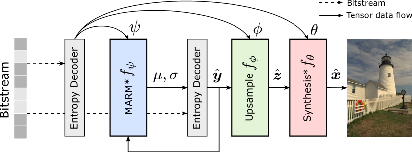
Figure 2. System architecture. The modules mark by * are proposed in this work to replace the original ones. $\psi$,$\phi$, $\theta$ are network parameters for MARM module, Upsample module and Synthesis module respectively. These parameters are decoded first to initialize the model. Then the MARM module decodes latents which are integer values matrices with pyramid shapes. Upsample module will transform these latents to a dense representation with shape $L\times H\times W$. Synthesis module transforms the dense tensor to image with $(r,g,b)$ channels and $H\times W$ shape. Note since the code length of $\psi,\phi,\theta$ is very small, we use original notation represents both quantized and unquantized version for simplicity.

When decompressing an image, the first step is decoding the network parameters $\psi$, $\phi$ and $\theta$ and initializing the whole model. Then $\hat{\boldsymbol{y}}$ is decoded from bitstream by $f_{\psi}$:

(4) $$\hat{\boldsymbol{y}}=f_{\psi}(\boldsymbol{b}),$$

where $\boldsymbol{b}$ represents bitstream. Like autoencoder codec, $f_{\psi}$ may have specific structure such as an autoregressive network (Leguay et al., 2023). Because making use of predictions from causal context of each symbol in this stage is very important to remove redundancy and reduce bit rate (Ballé et al., 2018; Minnen et al., 2018a; Minnen and Singh, 2020; Cheng et al., 2020). After that, a dense representation $\hat{\boldsymbol{z}}\in\mathbb{R}^{L\times H\times W}$ is obtained by the learnable upsampler $f_{\phi}$:

(5) $$\hat{\boldsymbol{z}}=f_{\phi}(\hat{\boldsymbol{y}}).$$

Finally, decoded image $\hat{\boldsymbol{x}}$ is reconstructed from $\hat{\boldsymbol{z}}$

(6) $$\hat{\boldsymbol{x}}=f_{\theta}(\hat{\boldsymbol{z}}).$$

For encoding stage, different from AE-based neural image codec, implicit neural representation based neural image codec does not require encoder. The encoding process of such methods is the process of training neural networks. Although the coding process is different, the final target function is the same:

(7) $$\mathcal{L}=D({\boldsymbol{x}},\hat{\boldsymbol{x}})+\lambda R(\hat{\boldsymbol{y}}),$$

where $D$ is distortion function such as mean squared error and $R$ approximate rate with entropy. Since the discrete value $\hat{\boldsymbol{y}}$ is non-differentiable, which is common to deep-learning compressor, we use a set of real value $\boldsymbol{y}$ with same shape as $\hat{\boldsymbol{y}}$ and a quantization function $Q$ in training

(8) $$\hat{\boldsymbol{y}}=Q(\boldsymbol{y}).$$

$Q$ could be either a fixed uniform scalar quantizer (Ballé et al., 2016) or $\epsilon$-STE quantizer (Leguay et al., 2023) according to training stage.

3.2. Mixed Autoregressive Model

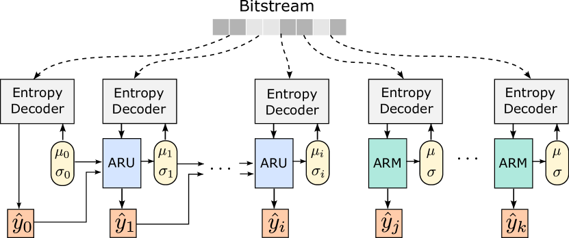
Figure 3. Network architecture of the MARM. Left part is channel-wise autoregressive model, which predict entropy parameters conditioned on previous latent. Right part correspond to inner-channel auto-regression model generation parameters pixel by pixel. Given the number of ARM blocks $M$ and total latents number $L$, we note $i=L-M-1$, $j=L-M$ and $k=L-1$ for simplicity. $\mu_{0}$ and $\sigma_{0}$ are initialized to tensor with 0 and $\exp(-0.5)$ respectively for all images. $\mu$ and $\sigma$ with subscription means the values output as a matrix rather than serially generated scalar for those without subscription.

Autoregressive network is widely used in casual context prediction (Minnen et al., 2018a; Leguay et al., 2023), which demonstrates the effectiveness of the structure in reducing redundancy of compressed representation. This is more clear if we decompose the second term of Eq. 7

(9) $$\begin{split}R(\hat{\boldsymbol{y}})=D_{KL}(q||p_{\psi})+H(\hat{\boldsymbol{y}}),\end{split}$$

where $D_{KL}$ stands for the Kullback-Leibler divergence and $H$ for Shannon’s entropy. The first term suggest the closer we approximate to real distribution $p$, the more bit we will save. In ARM model, $p_{\psi}$ is decomposed as:

(10) $$p_{\psi}(\hat{\boldsymbol{y}})=\prod_{l,i}p_{\psi}(\hat{y}_{l,i}|\mu_{l,i},\sigma_{l,i}),\text{where}\,\mu_{l,i},\sigma_{l,i}=f_{\psi}(\hat{y}_{l,<i}),$$

where $l$ means the $l$-th latent and $<i$ means all pixels in a flatten latent whose index is smaller than $i$. Obviously, the decoding proceeds pixel by pixel, which is time consuming and hard to parallelize. To alleviate such problem, our autoregressive upsampler (ARU) apply autoregressive decoding across latents. In other word, we use low-resolution latent to predict the decoding parameter of next high-resolution latent:

(11) $$p_{\psi}(\hat{\boldsymbol{y}})=\prod_{l}p_{\psi}(\hat{y}_{l}|\mu_{l},\sigma_{l}),$$

where $\mu_{l},\sigma_{l}=f_{\psi}(\hat{y}_{l-1},\mu_{l-1},\sigma_{l-1})$. This approach can significantly improve the parallelism of the autoregressive module and greatly enhance the computational performance. Similar technique is also used in some previous work (Reed et al., 2017).

While ARU block outperforms in efficiency, ARM can recognized more correlation between adjacent pixels because of locality inside each latent. So we integrate ARU and ARM to a Mixed AutoRegressive Model (MARM), as shown in Fig. 3. For low-resolution latents, which have more global information, ARU is used to accelerate decoding process. For high-resolution latents, we use ARM to capture more details such as textures. The ratio of two type blocks is controlled by a hyperparameter $M$, which means the number of ARM blocks in MARM. Note when $M=L$, the MARM becomes ARM.

3.3. Two Stages ARU

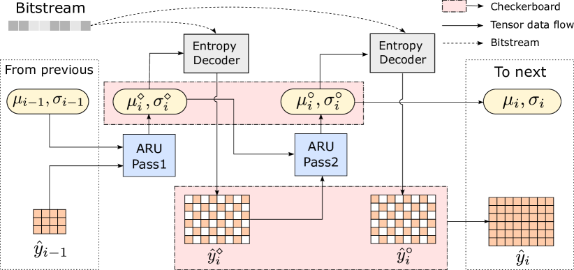
Figure 4. Network architecture of ARU. ARU uses previous parameter matrix $\mu_{i-1}$, $\sigma_{i-1}$ and latents as input. ARU pass1 output decoding parameters $\mu_{i}^{\diamond},\sigma_{i}^{\diamond}$ for anchors in latents. ARU Pass2 generate parameters for non-anchors conditioned on $\mu_{i}^{\diamond},\sigma_{i}^{\diamond}$ and anchors. Checkerboard means to merge anchor of the first tensor and non-anchor of the second tensor.

Although using low-resolution latent to predict higher-resolution ones is target to improve computational performance at the cost of reconstruction quality, the degradation can be reduced. Different from pixel-by-pixel correlation or cross resolution correlation, we can utilize the locality in only two pass in a checkerboard fashion. As shown in Fig. 4, we mark anchor in tensor $\hat{y}_{i}$, $\mu_{i}$, $\sigma_{i}$ (orange ones of $\hat{y}_{i}^{\diamond}$ in Fig.4 ) as $\hat{y}_{i}^{\diamond}$, $\mu_{i}^{\diamond}$, $\sigma_{i}^{\diamond}$, non-anchor (white ones of $\hat{y}_{i}^{\diamond}$ in Fig.4 ) as $\hat{y}_{i}^{\circ}$, $\mu_{i}^{\circ}$, $\sigma_{i}^{\circ}$ respectively. Following the notation, joint distribution of $\hat{y}_{i}$ can be written as

(12) $$\begin{split}p_{\psi}(\hat{y}_{i}|\mu_{i},\sigma_{i})&=p_{\psi}(\hat{y}_{i}^{\diamond}|\mu_{i},\sigma_{i})\cdot p_{\psi}(\hat{y}_{i}^{\circ}|\hat{y}_{i}^{\diamond},\mu_{i},\sigma_{i})\\ &=p_{\psi}(\hat{y}_{i}^{\diamond}|\mu_{i}^{\diamond},\sigma_{i}^{\diamond})\cdot p_{\psi}(\hat{y}_{i}^{\circ}|\mu_{i}^{\circ},\sigma_{i}^{\circ}).\end{split}$$

The anchor pixels only depend on information from previous low-resolution latent, and the correlation is fitted by $f_{\psi}^{\diamond}$:

(13) $$\mu_{i}^{\diamond},\sigma_{i}^{\diamond}=f_{\psi}^{\diamond}(\hat{y}_{i-1},\mu_{i-1},\sigma_{i-1}).$$

For decoding of non-anchor pixels, all previous information is available, including the decoded value of anchor $\hat{y}_{i}^{\diamond}$. As another form of making use of causal context information, ARU Pass2 can compute $\mu_{i}^{\circ}$ and $\sigma_{i}^{\circ}$ accordingly

(14) $$\mu_{i}^{\circ},\sigma_{i}^{\circ}=f_{\psi}^{\circ}(\hat{y}_{i}^{\diamond},\mu_{i}^{\diamond},\sigma_{i}^{\diamond}).$$

The idea of parallel predicting probability mass function of compressed representations have been investigated in some AE-based image or video codec (He et al., 2021; Li et al., 2023). Same as these method, INR codec also benefits from this design.

3.4. Mixed Synthesis module

Previous work have investigated the performance of full MLP (Ladune et al., 2023) and full convolutional network (Leguay et al., 2023) as synthesis. However the prior enforced by both structure may not apply for all input data. To enhance the generality of method, we combine MLP and convolution layer by a residual connection. This design further improves the reconstruction quality.

3.5. Complexity Analysis

In INR codec, the process of decoding latent takes part majority of decoding time in many cases. Given an image with $n=H\times W$ pixels, the total number latent pixels need to be decoded is $O(n)$. Because of serial decoding, time complexity is the same.

If we suppose parallel operations such as convolution operation over a feature map can be finished at $O(1)$, which is practical for not very large pictures in even low-power device with SIMD or NEON support, the decoding time complexity of MARM is $O((L-M)\log n+Mn)$. When $M=0$, the complexity of our method becomes $O(\log n)$, which surpass the previous work. When $M>L-M$, the complexity is similar to previous work. But in realistic setting, $n$ is finite, which means the constant factor is important as well. Actually, experiments support when $M\leq 2$, the acceleration is still significant.

4. Experiment

4.1. Datasets and Experiments Setup

The experiment use images from CLIC professional valid set and Kodak dataset. To ensure fairness in comparison, all learning-based model is implemented using PyTorch without special optimization. For AE-based models, we use the pre-trained model in CompressAI (Bégaint et al., 2020). Our model is implemented based on previous works (Ladune et al., 2023; Leguay et al., 2023), which use constriction package (Bamler, 2022) as entropy encoder. For simplicity, we only use newer version of COOL-CHIC (Leguay et al., 2023) as baseline since it has better decode quality and similar complexity. We note the work as COOL-CHICv2 in the rest of the paper.

We conduct our experiments on an edge device with quad-core Cortex-A57 and 4GB RAM, which is marked as edge. Considering the fast advancement of edge device, We also extend our experiments to server with high performance CPU. To simulate the computational resourece in edge device, all experiments is conducted on 1 CPU core at server, which is marked as server.

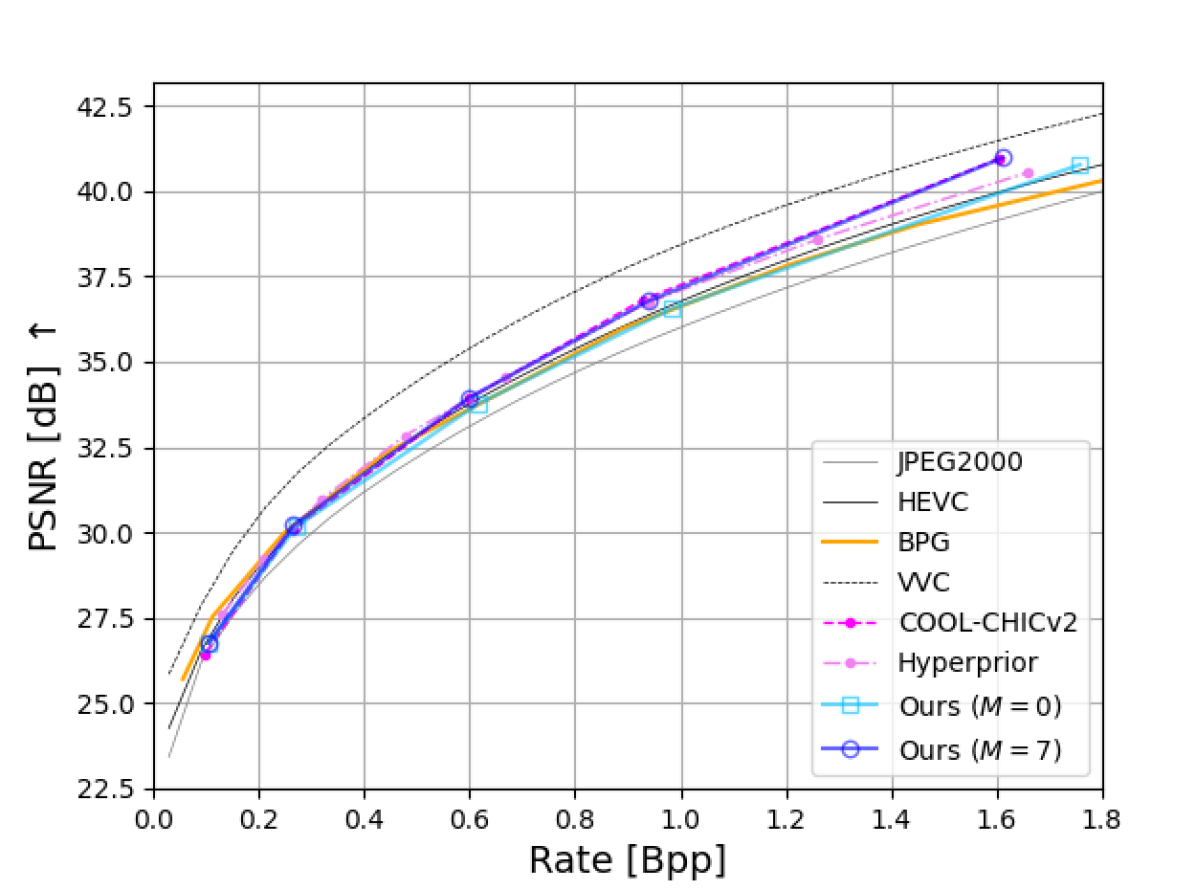
(a) RD curve of Kodak

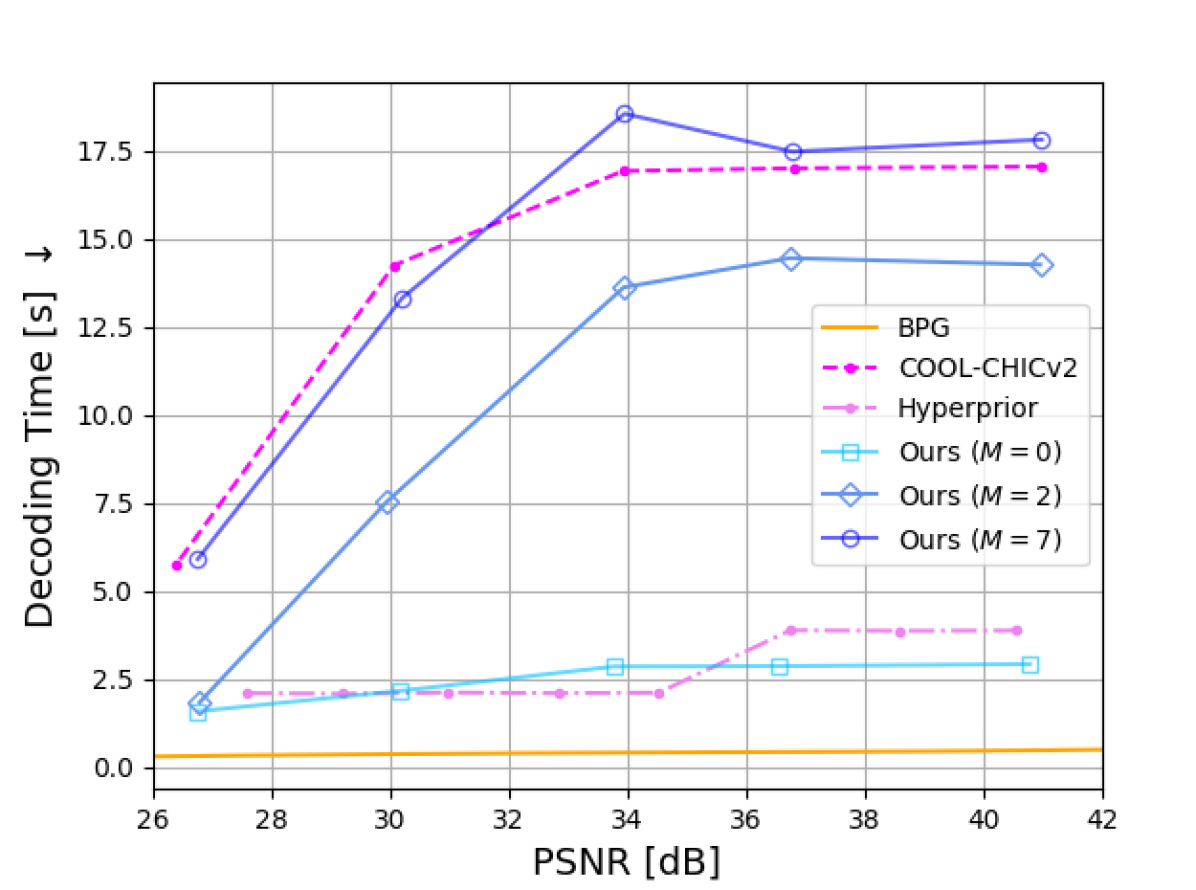
(b) Decoding time of Kodak on edge

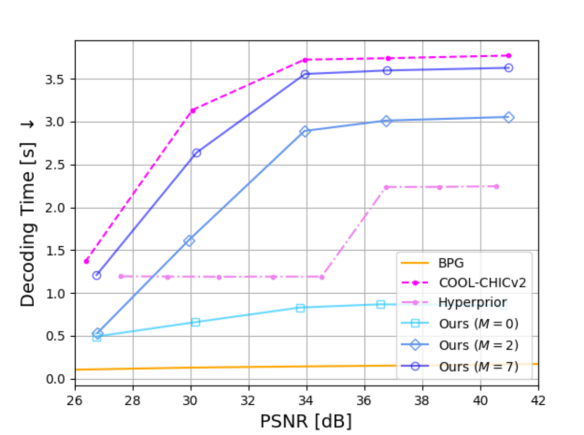
(c) Decoding time of Kodak on server

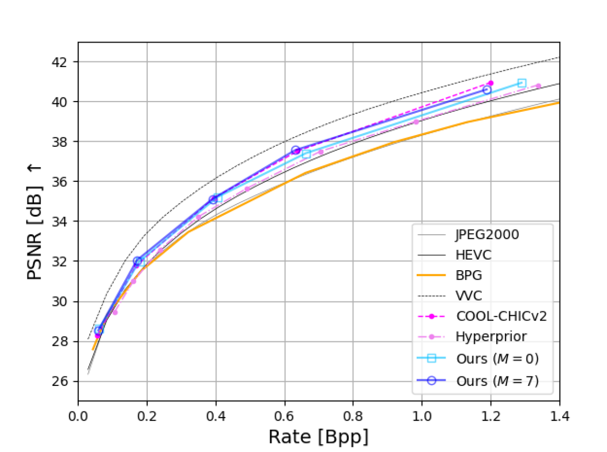
(d) RD curve of CLIC

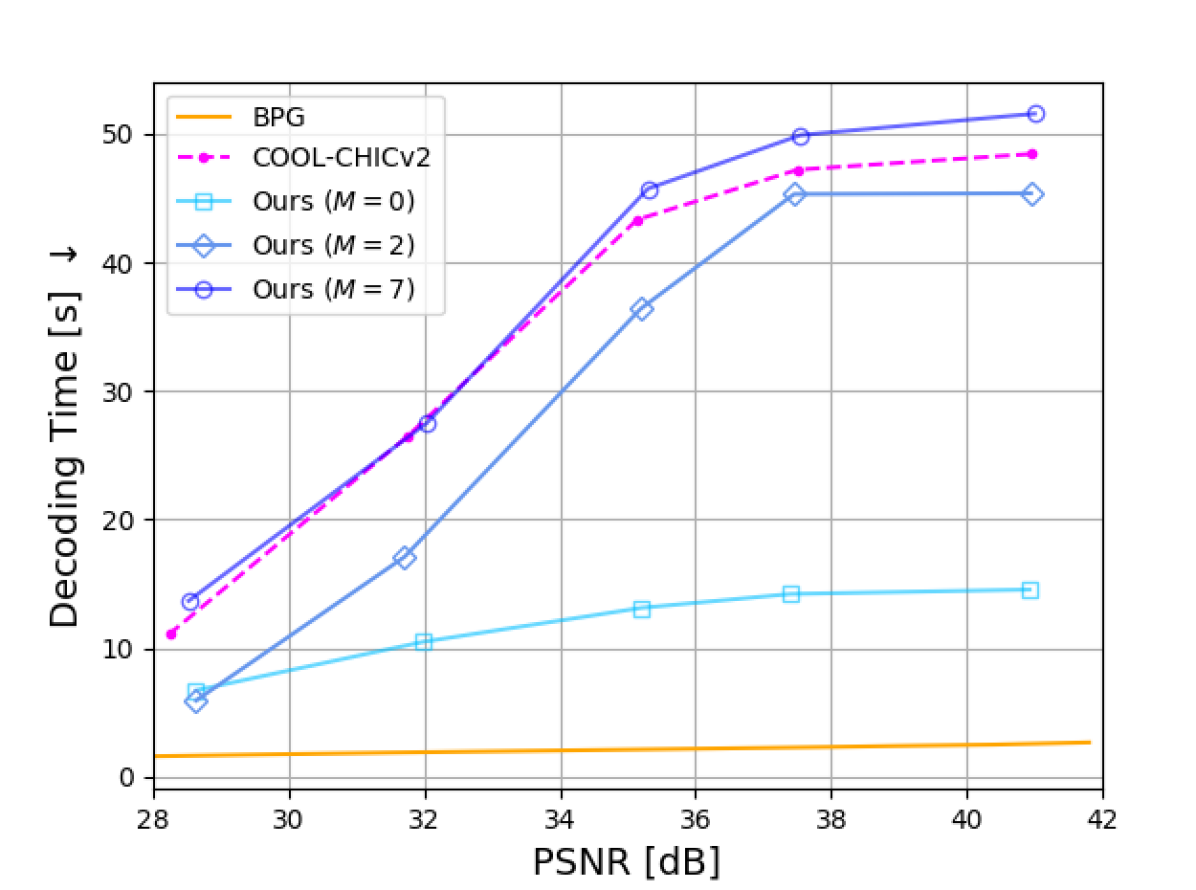
(e) Decoding time of CLIC on edge

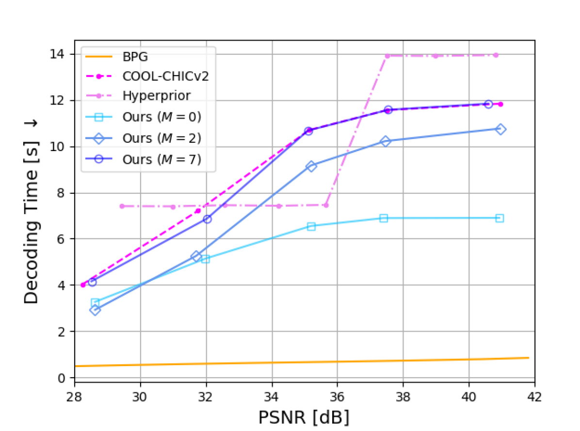
(f) Decoding time of CLIC on server

Figure 5. Main results of experiments. Fig. 5 and Fig. 5 shows the rate-distortion performance averaged over Kodak dataset and CLIC professional valid dataset respectively. Fig. 5, Fig. 5 , Fig. 5 and Fig. 5 shows the decoding time averaged over different dataset and different platform respectively. Hyperprior fails to decode on edge due to insufficient RAM. All COOL-CHIC-like methods aggregate the results over same $\lambda$. We observe our method achieves comparable reconstruction quality with COOL-CHICv2 on both kodak dataset and CLIC dataset when $M=7$. At the same time, we reduce time consumption of decoding on CPU by a large margin when use smaller $M$. If we relax quality restriction to set $M=0$ i.e. using pure ARU blocks in MARM module, the acceleration increases significantly.

4.2. Main Results

We use peak signal-to-noise ratios (PSNR) as quality measurement and bit-per-pixel (BPP) as coding efficiency metric. Fig. 5 and Fig. 5 illustrate the decompression quality results of our method. Not surprisingly, our method performs well on metric of reconstruction quality while fast method exceeds all COOL-CHIC-like method on decoding time.

To comprehensively evaluate the efficiency of a codec, we suggest to use the Time BD-rate (TBD-rate), which is a variant of BD-rate as the measurement. When calculating TBD-rate, We only need to replace BPP with decoding time in common BD-rate formula. More numerical results are shown in Table. LABEL:table:main_results. Our method achieve best quality or best decoding with different settings. We highlight that on CLIC dataset when $M=0$ our method outperforms Hyperprior model on both quality and decoding time.

Table 1. Numerical results of our method. Both BD rate and TBD rate are calculated relative to BPG on specific platform. Hyperprior fails to decode CLIC on edge as described before. Results marked by underline show our method surpasses Hyperprior on both quality and decoding time. FLOPs is normalized by pixels.

Method	Params	FLOPs	Kodak			CLIC
			BD Rate $\downarrow$	TBD/ Edge $\downarrow$	TBD/ Server $\downarrow$	BD Rate $\downarrow$	TBD/ Edge $\downarrow$	TBD/ Server $\downarrow$
Hyperprior	$5.90\times 10^{6}$	$1.041\times 10^{5}$	-2.4355	551.72	981.28	-8.3796	-	1314.42
COOL-CHICv2	$5.18\times 10^{5}$	$2.015\times 10^{3}$	-1.7798	3523.03	2245.73	-18.6662	1517.33	1251.07
Ours ($M=0$)	$5.72\times 10^{5}$	$2.481\times 10^{3}$	3.0817	522.71	443.40	-17.0435	469.45	779.20
Ours ($M=2$)	$5.28\times 10^{5}$	$2.864\times 10^{3}$	2.1380	2371.73	1469.43	-17.8065	1174.78	1014.03
Ours ($M=7$)	$5.27\times 10^{5}$	$2.889\times 10^{3}$	-2.9528	3576.42	2045.85	-20.5842	1610.31	1222.29

4.3. Ablation studys

As mentioned before, $M$ controls the ratio of ARU blocks and ARM blocks, and model performance is highly correlated to the parameter. Fig. 6 illustrates the overall decoding quality and efficiency.

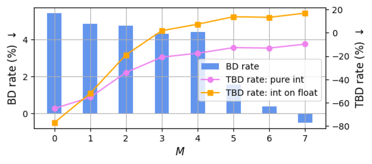
Figure 6. Quality and efficiency of different $M$. Both BD rate and TBD rate are computed relative to COOL-CHICv2 on Kodak dataset.

Table 2. Ablation results of the rate-distortion curve average over kodak dataset with different settings when $M=0$.

Module	Settings
Checkerboard	✓	✓
Mixed Synthesis	✓		✓
BD Rate $\downarrow$	0.0000	7.5453	7.1030

The trend of TBD-rate is easy to understand. More ARU block i.e. smaller $M$ leads to more significant acceleration. When $M$ increases, the performance improves accordingly. Especially when $M=7$, our model achieve state of the art RD performance. Besides, when $M=6$, the network of ARU is unnecessary, so the performance improves significantly comparing with $M<5$. For practical use, we suggest use smaller $M$ for better decoding speed and $M=L$ for best quality. Pure int and int-on-float are different decoding mode of entropy decode module. Since both mode output same result from same encoded bit stream, users may choose best one according to parameters setting and platform.

Table.LABEL:table:ablation illustrates the performance of checkerboard and our proposed new synthesis module. No checkerboard means we omit the second pass when decoding latent i.e. use $\mu_{i}^{\diamond},\sigma_{i}^{\diamond}$ directly to decode both anchors and no-anchors. No mixed synthesis means we use the original one in COOL-CHICv2. It is obvious that these two structures further improve the RD-performance.

5. Conclusion

This paper introduces a new module, MARM, designed to augment the current implicit neural representation image codec. Impressively, this is the first method to attain comparable performance in both reconstruction quality and decoding time. The MARM module enhances computational efficiency by utilizing the channel-wise autoregressive architecture in low-resolution latent and pixel-wise autoregressive mechanisms, ensuring the preservation of decompression quality. Our experimental results demonstrate that the alterations made result in a significant reduction in decoding time, without triggering substantial quality degradation.

References

- (1)
- Ballé et al. (2016) Johannes Ballé, Valero Laparra, and Eero P Simoncelli. 2016. End-to-end optimized image compression. arXiv preprint arXiv:1611.01704 (2016).
- Ballé et al. (2018) Johannes Ballé, David Minnen, Saurabh Singh, Sung Jin Hwang, and Nick Johnston. 2018. Variational image compression with a scale hyperprior. (2018).
- Bamler (2022) Robert Bamler. 2022. Understanding Entropy Coding With Asymmetric Numeral Systems (ANS): a Statistician’s Perspective. arXiv preprint arXiv:2201.01741 (2022).
- Bellard (2018) Fabrice Bellard. 2018. BPG Image format. https://bellard.org/bpg/
- Bégaint et al. (2020) Jean Bégaint, Fabien Racapé, Simon Feltman, and Akshay Pushparaja. 2020. CompressAI: a PyTorch library and evaluation platform for end-to-end compression research. (2020).
- Chen et al. (2021) Yinbo Chen, Sifei Liu, and Xiaolong Wang. 2021. Learning continuous image representation with local implicit image function. In Proceedings of the IEEE/CVF conference on computer vision and pattern recognition. 8628–8638.
- Chen and Zhang (2019) Zhiqin Chen and Hao Zhang. 2019. Learning implicit fields for generative shape modeling. In Proceedings of the IEEE/CVF Conference on Computer Vision and Pattern Recognition. 5939–5948.
- Cheng et al. (2020) Zhengxue Cheng, Heming Sun, Masaru Takeuchi, and Jiro Katto. 2020. Learned image compression with discretized gaussian mixture likelihoods and attention modules. In Proceedings of the IEEE/CVF conference on computer vision and pattern recognition. 7939–7948.
- Dupont et al. (2021a) Emilien Dupont, Adam Goliński, Milad Alizadeh, Yee Whye Teh, and Arnaud Doucet. 2021a. Coin: Compression with implicit neural representations. arXiv preprint arXiv:2103.03123 (2021).
- Dupont et al. (2022) Emilien Dupont, Hrushikesh Loya, Milad Alizadeh, Adam Golinski, Yee Whye Teh, and Arnaud Doucet. 2022. Coin++: Data agnostic neural compression. arXiv preprint arXiv:2201.12904 1, 2 (2022), 4.
- Dupont et al. (2021b) Emilien Dupont, Yee Whye Teh, and Arnaud Doucet. 2021b. Generative Models as Distributions of Functions. (2021).
- Goyal (2001) V. K Goyal. 2001. Theoretical foundations of transform coding. IEEE Signal Processing Magazine 18, 5 (2001), 9–21.
- He et al. (2022) Dailan He, Ziming Yang, Weikun Peng, Rui Ma, Hongwei Qin, and Yan Wang. 2022. ELIC: Efficient Learned Image Compression with Unevenly Grouped Space-Channel Contextual Adaptive Coding. arXiv e-prints (2022).
- He et al. (2021) Dailan He, Yaoyan Zheng, Baocheng Sun, Yan Wang, and Hongwei Qin. 2021. Checkerboard context model for efficient learned image compression. In Proceedings of the IEEE/CVF Conference on Computer Vision and Pattern Recognition. 14771–14780.
- Ladune et al. (2023) Théo Ladune, Pierrick Philippe, Félix Henry, Gordon Clare, and Thomas Leguay. 2023. Cool-chic: Coordinate-based low complexity hierarchical image codec. In Proceedings of the IEEE/CVF International Conference on Computer Vision. 13515–13522.
- Leguay et al. (2023) Thomas Leguay, Théo Ladune, Pierrick Philippe, Gordon Clare, and Félix Henry. 2023. Low-complexity Overfitted Neural Image Codec. arXiv preprint arXiv:2307.12706 (2023).
- Li et al. (2023) Jiahao Li, Bin Li, and Yan Lu. 2023. Neural video compression with diverse contexts. In Proceedings of the IEEE/CVF Conference on Computer Vision and Pattern Recognition. 22616–22626.
- Mildenhall et al. (2020) Ben Mildenhall, Pratul P. Srinivasan, Matthew Tancik, Jonathan T. Barron, Ravi Ramamoorthi, and Ren Ng. 2020. NeRF: Representing Scenes as Neural Radiance Fields for View Synthesis.
- Minnen et al. (2018a) David Minnen, Johannes Ballé, and George Toderici. 2018a. Joint Autoregressive and Hierarchical Priors for Learned Image Compression. (2018).
- Minnen and Singh (2020) David Minnen and Saurabh Singh. 2020. Channel-wise Autoregressive Entropy Models for Learned Image Compression.
- Minnen et al. (2018b) David Minnen, George Toderici, Saurabh Singh, Sung Jin Hwang, and Michele Covell. 2018b. Image-dependent local entropy models for learned image compression. In 2018 25th IEEE International Conference on Image Processing (ICIP). IEEE, 430–434.
- Müller et al. (2022) Thomas Müller, Alex Evans, Christoph Schied, and Alexander Keller. 2022. Instant neural graphics primitives with a multiresolution hash encoding. ACM Transactions on Graphics (ToG) 41, 4 (2022), 1–15.
- Park et al. (2019) Jeong Joon Park, Peter Florence, Julian Straub, Richard Newcombe, and Steven Lovegrove. 2019. Deepsdf: Learning continuous signed distance functions for shape representation. In Proceedings of the IEEE/CVF conference on computer vision and pattern recognition. 165–174.
- Reed et al. (2017) Scott Reed, Aäron Oord, Nal Kalchbrenner, Sergio Gómez Colmenarejo, Ziyu Wang, Yutian Chen, Dan Belov, and Nando Freitas. 2017. Parallel multiscale autoregressive density estimation. In International conference on machine learning. PMLR, 2912–2921.
- Strümpler et al. (2022) Yannick Strümpler, Janis Postels, Ren Yang, Luc Van Gool, and Federico Tombari. 2022. Implicit neural representations for image compression. In European Conference on Computer Vision. Springer, 74–91.
- Van den Oord et al. (2016) Aaron Van den Oord, Nal Kalchbrenner, Lasse Espeholt, Oriol Vinyals, Alex Graves, et al. 2016. Conditional image generation with pixelcnn decoders. Advances in neural information processing systems 29 (2016).
- Van Den Oord et al. (2016) Aäron Van Den Oord, Nal Kalchbrenner, and Koray Kavukcuoglu. 2016. Pixel recurrent neural networks. In International conference on machine learning. PMLR, 1747–1756.
- Wallace (1992) Gregory K Wallace. 1992. The JPEG still picture compression standard. IEEE transactions on consumer electronics 38, 1 (1992), xviii–xxxiv.
- Wang et al. (2003) Zhou Wang, Eero P Simoncelli, and Alan C Bovik. 2003. Multiscale structural similarity for image quality assessment. In The Thrity-Seventh Asilomar Conference on Signals, Systems & Computers, 2003, Vol. 2. Ieee, 1398–1402.