Work statistics at first-passage times

Abstract

We investigate the work fluctuations in an overdamped non-equilibrium process that is stopped at a stochastic time. The latter is characterized by a first passage event that marks the completion of the non-equilibrium process. In particular, we consider a particle diffusing in one dimension in the presence of a time-dependent potential $U(x,t)=k|x-vt|^{n}/n$, where $k>0$ is the stiffness and $n>0$ is the order of the potential. Moreover, the particle is confined between two absorbing walls, located at $L_{\pm}(t)$, that move with a constant velocity $v$ and are initially located at $L_{\pm}(0)=\pm L$. As soon as the particle reaches any of the boundaries, the process is said to be completed and here, we compute the work done $W$ by the particle in the modulated trap upto this random time. Employing the Feynman-Kac path integral approach, we find that the typical values of the work scale with $L$ with a crucial dependence on the order $n$. While for $n>1$, we show that $W\sim L^{1-n}~{}\exp\left[\left({kL^{n}}/{n}-vL\right)/D\right]$ for large $L$, we get an algebraic scaling of the form $W\sim L^{n}$ for the $n<1$ case. The marginal case of $n=1$ is exactly solvable and our analysis unravels three distinct scaling behaviours: (i) $W\sim L$ for $v>k$, (ii) $W\sim L^{2}$ for $v=k$ and (iii) $W\sim\exp\left[{-(v-k)L}\right]$ for $v<k$. For all cases, we also obtain the probability distribution associated with the typical values of $W$. Finally, we observe an interesting set of relations between the relative fluctuations of the work done and the first-passage time for different $n$ – which we argue physically. Our results are well supported by the numerical simulations.

1 Introduction

Stochastic thermodynamics generally provides a thermodynamic framework to nano-scaled systems subjected to thermal fluctuations, even when they are driven arbitrarily far from the equilibrium [1, 2, 3]. Contrary to classical equilibrium thermodynamics, one now has well-defined probability distributions of the thermodynamic quantities such as heat, work and entropy production [4, 5]. Furthermore, stochastic thermodynamics can be used to derive several fundamental relations such as fluctuation theorems [6, 7, 8, 9, 10, 11, 12], uncertainty relations [13, 14, 15, 16, 17, 18, 19, 20, 21, 22, 23] and thermodynamic speed limits [24, 25, 26, 27, 28, 29, 30, 31, 32, 33, 34, 35, 36].

Recently, there has been a growing interest in the study of the thermodynamic quantities until a particular event of interest has occurred for the first time [37, 38, 39, 40, 41, 42, 43, 44, 45, 46, 47, 48, 23]. Examples include the escape of a colloidal particle from a metastable state or stretching of a polymer till a certain length is attained [41]. Since the underlying dynamics is stochastic, the time at which these events take place also varies from realisation to realisation. This drastically changes the properties of the thermodynamic quantities compared to situations where the observation time is fixed for all realisations. For instance, the bound on the average work picks up a non-trivial correction term due to the fact that the system is generally out of equilibrium at the end of the first-passage time [41]. Similar observation has also been made for the efficiency of heat engines [40]. In fact, based on the martingale theory, many new results on the integral fluctuation theorem and stopping times for entropy production have been analytically obtained [49]. Despite these general results, the number of thermodynamic first-passage problems that have been solved exactly, seems to be very limited. In this paper, we aim to partially fill this gap by studying an analytically tractable class of models, where one can get exact results for the moment generating function associated with the mechanical work.

In order to study this, we reformulate the work done as a first-passage functional of the stochastic process [50]. Statistical properties of such functionals have been quite extensively studied in the literature by deploying the celebrated Feynman-Kac formalism suitably adapted for first-passage problems [51]. Based on this formalism, these functionals have been shown to have many applications in fields ranging from queue theory [52], sandpile and percolation models [53, 54] to disordered systems [55], among others [56, 57, 58]. Moreover, they have been studied for diverse stochastic processes such as diffusion and drift-diffusion [59, 60, 61, 62], random acceleration [63], Lévy process [64], Ornstein-Uhlenbeck particle [65, 66] and resetting processes [67, 68]. In this paper, we are interested in using these tools and techniques to calculate the moments and the distribution of the work done by a diffusing particle subjected to a time-dependent potential $U(x,t)=\frac{k}{n}|x-vt|^{n}$ with order $n>0$. In particular, we show that the work can be reformulated as a first-passage functional and one can then employ the Feynman-Kac formalism to investigate its statistical properties.

The rest of the paper is structured as follows: In Section 2, we introduce our model and present a general formalism to study the work done. We first focus on the analytically tractable cases of the linear potential $(n=1)$ in Section 3 and the harmonic potential ($n=2$) in Section 4. The insights gained from these two cases become instrumental in dealing with the general $n$ in Section 5. We then discuss an interesting relation between the work done and the first-passage time in Section 6. Finally, in Section 7, we present the conclusion and make some future remarks.

2 Model and general formulation of the problem

We consider a one-dimensional diffusing particle whose position, in presence of a time-dependent potential $U(x,t)$, evolves according to an overdamped Langevin equation

$$\frac{dx}{dt}=-\frac{\partial U(x,t)}{\partial x}+\sqrt{2D}~{}\eta(t),$$ (1)

where $\eta(t)$ is the Gaussian white noise with zero mean and delta temporal correlation and $D$ is the diffusion constant. The initial position of the particle will be denoted as $x_{0}$. Moreover, we choose the potential $U(x,t)$ to be a confining potential with stiffness $k~{}(>0)$ and we let it move with a constant velocity $v~{}(>0)$:

$$U(x,t)=\frac{k}{n}~{}\big{|}x-vt\big{|}^{n},~{}~{}~{}~{}~{}\text{with }n>0.$$ (2)

Finally, we will assume the existence of two absorbing walls located at positions $L_{\pm}(t)$ that themselves move with the same constant velocity $v$, i.e. $L_{\pm}(t)=\pm L+vt$, with $-L<x_{0}<L$.

As mentioned in the introduction, we are interested in the work distribution of first-passage time problems. Here, we allow the particle to move until it touches one of the absorbing boundaries at $L_{\pm}(t)$. Let us denote this time by $t_{f}$ and the corresponding trajectory as $\{x(\tau)\}$ with $0\leq\tau\leq t_{f}$. We then calculate the work done up to time $t_{f}$ as [4, 69, 70, 71]

$$W(x_{0}) =\int_{0}^{t_{f}}d\tau~{}\frac{\partial U(x(\tau),\tau)}{\partial\tau}=-kv\int_{0}^{t_{f}}d\tau~{}\operatorname{sgn}\Big{(}x(\tau)-v\tau\Big{)}~{}\big{|}x(\tau)-v\tau\big{|}^{n-1},$$ (3)

$$\text{with }t_{f} =\text{min}\{\ \tau:x(\tau)\geq L_{+}(\tau),~{}\text{or }x(\tau)\leq L_{-}(\tau)\}.$$ (4)

Since the motion is random, we get different values of $t_{f}$ for different realisations. This indicates that in contrast to the usual case of fixed observation time, the definition of work in Eq. (3) possesses two sources of stochasticity - one arises due to the random trajectory $\{x(\tau)\}$ and the other stems from random first-passage time $t_{f}$.

In order to derive the statistics of $W(x_{0})$, we reformulate the work done as a first-passage functional which has been extensively studied in the literature [50]. To see this, let us first perform a change of variable as

$$\xi(t)=x(t)-vt,$$ (5)

and recast the Langevin equation and the work done in terms of this new co-moving variable:

$$\frac{\partial\xi}{\partial t}=-k\operatorname{sgn}\left(\xi(t)\right)\big{|}\xi(t)\big{|}^{n-1}-v+\sqrt{2D}~{}\eta(t),$$ (6)

$$W(x_{0})=-kv\int_{0}^{t_{f}}d\tau~{}\operatorname{sgn}\Big{(}\xi(\tau)\Big{)}~{}|\xi(\tau)|^{n-1}.$$ (7)

Meanwhile, the first-passage time $t_{f}$, in the co-moving frame, simply becomes the time at which the particle moves out of the fixed interval $[-L,L]$ for the first time. Therefore, by suitably defining the variable $\xi(t)$, we have been able to recast the entire problem with fixed absorbing walls. Following [51, 50], one can now derive a backward differential equation for the moment generating function

$$\centering Q(p,\xi_{0})=\left\langle e^{-pW(\xi_{0})}\right\rangle=\left\langle\exp\left[kpv\int_{0}^{t_{f}}d\tau~{}\operatorname{sgn}\Big{(}\xi(\tau)\Big{)}~{}\big{|}\xi(\tau)\big{|}^{n-1}\right]\right\rangle,\@add@centering$$ (8)

with $\xi_{0}=\xi(t=0)=x_{0}$ and the averaging $\left\langle...\right\rangle$ involves averaging both with respect to the trajectories as well as the first-passage time $t_{f}$. To do this, we now look at a trajectory of $\xi(\tau)$ from $\tau=0$ to $\tau=t_{f}$ and break it into two parts: (i) a left interval $[0,\Delta t]$ and (ii) a right interval $[\Delta t,t_{f}]$ with $\Delta t\to 0$. At the end of the left interval, the variable $\xi(t)$ takes the value $\xi(\Delta t)=\xi_{0}-\left[k\operatorname{sgn}(\xi_{0})|\xi_{0}|^{n-1}+v\right]\Delta t+\sqrt{2D}~{}\Delta t~{}\eta(0)$. In the remaining time interval $(t_{f}-\Delta t)$, the particle starting from $\xi(\Delta t)$ moves out of the interval $[-L,L]$. Therefore, decomposing the integral in Eq. (8) as $\int_{0}^{t_{f}}=\int_{0}^{\Delta t}+\int_{\Delta t}^{t_{f}}$, we obtain

$$Q(p,\xi_{0}) \simeq\left\langle\exp\left[kpv\operatorname{sgn}(\xi_{0})\big{|}\xi_{0}\big{|}^{n-1}\Delta t\right]~{}Q(p,\xi(\Delta t))\right\rangle,$$ (9)

$$\simeq\left[1+kpv\operatorname{sgn}(\xi_{0})\big{|}\xi_{0}\big{|}^{n-1}\Delta t\right]~{}\left\langle Q(p,\xi(\Delta t))\right\rangle.$$ (10)

Inserting the expression of $\xi(\Delta t)$ and performing the expansion in $\Delta t$, we obtain the following differential equation for $Q(p,\xi_{0})$ as $\Delta t\to 0$:

$$D\frac{\partial^{2}Q(p,\xi_{0})}{\partial\xi_{0}^{2}}-\Big{(}kf_{n}(\xi_{0})+v\Big{)}\frac{\partial Q(p,\xi_{0})}{\partial\xi_{0}}+kpvf_{n}(\xi_{0})~{}Q(p,\xi_{0})=0,$$ (11)

where $f_{n}(\xi_{0})=\operatorname{sgn}(\xi_{0})\big{|}\xi_{0}\big{|}^{n-1}$. This equation has to be solved in the domain $-L\leq\xi_{0}\leq L$ and it a differential equation in the initial position $\xi_{0}$. This approach is referred to as a“backward” approach as it involves varying the initial position instead of the final one. Moreover it is a second order differential equation. Thus, we need two boundary conditions to solve it. These conditions can be obtained by analysing the behaviour of $Q(p,\xi_{0})$ at $\xi_{0}=\pm L$. For these two cases, the particle is already at the edge of the interval and gets instantly absorbed. Thus, for both cases, we have $t_{f}=0$ which implies $W(\pm L)=0$ from Eq. (7). Plugging this in Eq. (8), we obtain

$$Q(p,\xi_{0}=\pm L)=1.$$ (12)

The goal now is to solve the backward Eq. (11) with these boundary conditions and then utilize it to obtain the moments of $W(x_{0})$ as

$$\left\langle W^{m}(\xi_{0})\right\rangle=(-1)^{m}\frac{\partial^{m}Q(p,\xi_{0})}{\partial p^{m}}\bigg{|}_{p=0}.$$ (13)

One can also obtain the full probability distribution by performing the inverse transformation with respect to the $p$-variable in Eq. (8). In what follows, we first illustrate this rigorously for the analytically tractable cases $n=1$ and $n=2$. Then, we will combine the intuition gained in these solvable cases with Eq. (11) to derive some general results for arbitrary $n$.

3 Linear potential $(n=1)$

Let us first look at the $n=1$ case for which we can solve the backward Eq. (11) analytically. For this case, the Langevin equation (6) takes the form

$$\frac{\partial\xi}{\partial t}=-k\operatorname{sgn}\left(\xi(t)\right)-v+\sqrt{2D}~{}\eta(t).$$ (14)

In essence, this is a drift-diffusion process in which the particle experiences two distinct drifts. The first one involves a drift with a magnitude $k$, that tries to pull the particle back to the origin. The second one involves a drift of magnitude $v$ that tends to take the particle away from the origin along the negative $x$ direction. The behaviour of the particle varies depending on which of the two terms dominate. To see this in the context of work done, let us proceed to solve the backward Eq. (11). Depending on the sign of the initial position $\xi_{0}$, we can split the backward equation as

$$\begin{cases}\left[\partial^{2}_{\xi_{0}}-\mu\partial_{\xi_{0}}+\frac{kvp}{D}\right]Q(p,\xi_{0})=0\text{ , for }\xi_{0}>0\\ \left[\partial^{2}_{\xi_{0}}-\gamma\partial_{\xi_{0}}-\frac{kvp}{D}\right]Q(p,\xi_{0})=0\text{ , for }\xi_{0}<0,\end{cases}$$ (15)

where $\mu=(v+k)/D$, $\gamma=(v-k)/D$. Solving this set of equations yields

$$\centering Q(p,\xi_{0})\@add@centering =\begin{cases}K_{1}(p)e^{\lambda_{+}(p)\xi_{0}}+K_{2}(p)e^{\lambda_{-}(p)\xi_{0}}\text{ , for }\xi_{0}>0\\ K_{3}(p)e^{\sigma_{+}(p)\xi_{0}}+K_{4}(p)e^{\sigma_{-}(p)\xi_{0}}\text{ , for }\xi_{0}<0,\end{cases}$$ (16)

$$\text{with }\lambda_{\pm}(p) =\frac{1}{2}\left(\mu\pm\sqrt{\mu^{2}-\frac{4kvp}{D}}\right)~{}\text{and }\sigma_{\pm}(p)=\frac{1}{2}\left(\gamma\pm\sqrt{\gamma^{2}+\frac{4kvp}{D}}\right).$$ (17)

To compute the $K(p)$-functions, we will need four conditions. Two of these are the boundary conditions $Q(p,\xi_{0}=\pm L)$ which are given in Eq. (12). The other two can be obtained by looking at the behaviour of $Q(p,\xi_{0})$ and its derivative in the vicinity of $\xi_{0}=0$. Integrating the backward Eq. (11) from $-\epsilon$ to $+\epsilon$ and then taking $\epsilon\to 0^{+}$, we obtain

$$\centering\begin{cases}Q(p,\xi_{0}\to 0^{+})=Q(p,\xi_{0}\to 0^{-}),\\ \partial_{\xi_{0}}Q(p,\xi_{0})\big{|}_{\xi_{0}\to 0^{+}}=\partial_{\xi_{0}}Q(p,\xi_{0})\big{|}_{\xi_{0}\to 0^{-}}.\end{cases}\@add@centering$$ (18)

Using these conditions, it is possible to compute all $K(p)$-functions as

$$K_{1}(p) =\frac{\left(\sigma_{-}-\sigma_{+}\right)e^{\lambda_{-}L}+\left(\sigma_{+}-\lambda_{-}\right)e^{-\sigma_{-}L}+\left(\lambda_{-}-\sigma_{-}\right)e^{-\sigma_{+}L}}{e^{\lambda_{+}L}[\left(\sigma_{+}-\lambda_{-}\right)e^{-\sigma_{-}L}+\left(\lambda_{-}-\sigma_{-}\right)e^{-\sigma_{+}L}]+e^{\lambda_{-}L}[\left(\lambda_{+}-\sigma_{+}\right)e^{-\sigma_{-}L}+\left(\sigma_{-}-\lambda_{+}\right)e^{-\sigma_{+}L}]},$$

$$K_{2}(p) =\frac{\left(\sigma_{+}-\sigma_{-}\right)e^{\lambda_{+}L}+\left(\lambda_{+}-\sigma_{+}\right)e^{-\sigma_{-}L}+\left(\sigma_{-}-\lambda_{+}\right)e^{-\sigma_{+}L}}{e^{\lambda_{+}L}[\left(\sigma_{+}-\lambda_{-}\right)e^{-\sigma_{-}L}+\left(\lambda_{-}-\sigma_{-}\right)e^{-\sigma_{+}L}]+e^{\lambda_{-}L}[\left(\lambda_{+}-\sigma_{+}\right)e^{-\sigma_{-}L}+\left(\sigma_{-}-\lambda_{+}\right)e^{-\sigma_{+}L}]},$$

$$K_{3}(p) =\frac{\left(\lambda_{+}-\sigma_{-}\right)e^{\lambda_{-}L}+\left(\sigma_{-}-\lambda_{-}\right)e^{\lambda_{+}L}+\left(\lambda_{-}-\lambda_{+}\right)e^{-\sigma_{-}L}}{e^{\lambda_{+}L}[\left(\sigma_{+}-\lambda_{-}\right)e^{-\sigma_{-}L}+\left(\lambda_{-}-\sigma_{-}\right)e^{-\sigma_{+}L}]+e^{\lambda_{-}L}[\left(\lambda_{+}-\sigma_{+}\right)e^{-\sigma_{-}L}+\left(\sigma_{-}-\lambda_{+}\right)e^{-\sigma_{+}L}]},$$

$$K_{4}(p) =\frac{\left(\lambda_{+}-\sigma_{+}\right)e^{\lambda_{-}L}+\left(\sigma_{+}-\lambda_{-}\right)e^{\lambda_{+}L}+\left(\lambda_{-}-\lambda_{+}\right)e^{-\sigma_{+}L}}{e^{\lambda_{+}L}[\left(\sigma_{+}-\lambda_{-}\right)e^{-\sigma_{-}L}+\left(\lambda_{-}-\sigma_{-}\right)e^{-\sigma_{+}L}]+e^{\lambda_{-}L}[\left(\lambda_{+}-\sigma_{+}\right)e^{-\sigma_{-}L}+\left(\sigma_{-}-\lambda_{+}\right)e^{-\sigma_{+}L}]},$$

and inserting them in Eq. (16), we get for $\xi_{0}=0$

$$Q(p,0)=K_{1}(p)+K_{2}(p).$$ (19)

This gives us the exact form of the moment-generating function for the case of linear potential. By taking derivative of Eq. (19) suitably with respect to $p$, we can now obtain all moments of the work $W$. For instance, we find the mean as

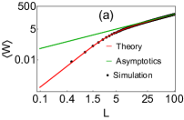
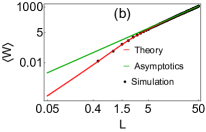
Figure 1: Plots of the mean work $\left\langle W\right\rangle$ for the linear $n=1$ potential for (a) $\gamma>0~{}(v=1,~{}k=0.5)$, (b) $\gamma=0~{}(v=k=1)$ and $\gamma<0~{}(v=0.5,~{}k=1)$. For all panels, the red curve corresponds to the exact result in Eq. (20) and the green curve is the asymptotic expression in Eq. (21). We have chosen $D=1$.

$$\centering\left\langle W\right\rangle=\left(\frac{kv}{\gamma{D}\mu}\right)\frac{(\gamma+\mu)\left[e^{\mu L}+e^{-\gamma L}-e^{(\mu-\gamma)L}-1\right]-\gamma\mu L\left[e^{\mu L}-e^{-\gamma L}\right]}{\gamma\left[1-e^{\mu L}\right]-\mu\left[1-e^{-\gamma L}\right]}.\@add@centering$$ (20)

Here, we have introduced the simplified notation $\left\langle W^{m}\right\rangle$ instead of $\left\langle W^{m}(0)\right\rangle$. To gain some physical insights, let us look at the asymptotic behaviour of this mean as $L$ becomes large. This behaviour turns out to crucially depend on the signature of the parameter $\gamma$ and we find

$$\left\langle W\right\rangle\simeq\begin{cases}\frac{kvL}{\gamma D},~{}~{}~{}~{}~{}~{}~{}~{}~{}~{}~{}~{}~{}~{}\text{for }\gamma>0,\\ \frac{v^{2}L^{2}}{2D},~{}~{}~{}~{}~{}~{}~{}~{}~{}~{}~{}~{}~{}\text{for }\gamma=0,\\ \frac{2kv^{2}}{\gamma^{2}D^{2}\mu}~{}e^{-\gamma L},~{}~{}~{}~{}\text{for }\gamma<0.\end{cases}$$ (21)

Physically, for $\gamma<0$ (or equivalently $v<k$), the drift $v$ in Eq. (6) is not strong enough for the particle to overcome the force $k$. Thus, the particle typically takes exponentially large time to reach the absorbing walls which, in turn, gives rise to exponentially large value of the work. On the other hand, for $\gamma>0$ (or equivalently $v>k$), the particle can easily overcome the constant force and reach the absorbing walls with relatively high probability. Therefore, we get smaller values of the work which scales linearly with $L$. For the marginal case $\gamma=0$, we anticipate the scaling to lie somewhere in between $\gamma>0$ and $\gamma<0$ cases. In Figure 1, we have compared these asymptotic results and their exact expressions in Eq. (20) with the numerical simulation of the Langevin equation (1).

After analysing the mean, we now proceed to compute the full probability distribution of the work. For this, we need to perform the inverse Laplace transformation of $Q(p,0)$ in Eq. (19). For large $L$, we saw that the work typically takes a large positive value for all values of $\gamma$. In terms of $p$-variable, this translates to taking small $p$ limit of the moment generating function. Taking $p\to 0$ limit in Eq. (19), we find that $Q(p,0)$ also takes different forms depending on the signature of $\gamma$. In A, we have rigorously derived these forms for large $L$ and found

$$Q(p,0)\simeq\begin{cases}\exp\left(\frac{\gamma L}{2}-\frac{L}{2}\sqrt{\gamma^{2}+\frac{4vkp}{D}}\right),~{}~{}~{}~{}~{}~{}~{}~{}~{}~{}~{}~{}~{}~{}~{}~{}~{}~{}~{}~{}\text{for }\gamma>0,\\ \\ \frac{\mu\left\{\exp(2\alpha L\sqrt{p})-1\right\}+2\beta\sqrt{p}\exp(\alpha L\sqrt{p})}{\mu\left\{\exp(2\alpha L\sqrt{p})-1\right\}+\beta\sqrt{p}~{}\left\{\exp(2\alpha L\sqrt{p})+1\right\}},~{}~{}~{}~{}~{}~{}~{}~{}~{}~{}\text{for }\gamma=0,\\ \\ \left[1+p\left\langle W\right\rangle\left(1+\frac{kvL}{D\big{|}\gamma\big{|}}p\right)\right]^{-1},~{}~{}~{}~{}~{}~{}~{}~{}~{}~{}~{}~{}~{}~{}~{}~{}~{}\text{for }\gamma<0,\end{cases}$$ (22)

where $\alpha=v/\sqrt{D}$ and $\beta=\alpha\left(e^{\mu L}-1\right)$. For $\gamma\neq 0$, we can perform the inverse Laplace transformation explicitly and obtain the distribution of work to be

$$P(W)\simeq\begin{cases}L\sqrt{\frac{kv}{4\pi DW^{3}}}\exp\left[-\frac{D\gamma^{2}}{4kvW}\left(W-\frac{kvL}{D}\right)^{2}\right],~{}~{}~{}~{}~{}\text{for }\gamma>0,\\ \\ \frac{1}{\left\langle W\right\rangle}\left[\exp\left(-\frac{W}{\left\langle W\right\rangle}\right)-\exp\left(-\frac{D\big{|}\gamma\big{|}W}{kvL}\right)\right],~{}~{}~{}~{}\text{for }\gamma<0.\end{cases}$$ (23)

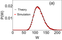
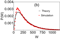
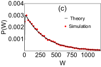
Figure 2: Distribution of the work done by the particle for the linear potential $(n=1)$ for (a) $\gamma>0~{}(v=1,~{}k=0.5,~{}L=120)$, (b) $\gamma=0~{}(v=k=1,~{}L=25)$ and $\gamma<0~{}(v=0.3,~{}k=1,~{}L=10)$. The theoretical expressions are given in Eqs. (23) and (25). We have chosen $D=1$.

On the other hand, for $\gamma=0$, we perform the expansion

$$Q(p,0)\simeq\frac{1}{1+\frac{L^{2}\alpha^{2}}{2}p+\frac{L^{4}\alpha^{4}}{24}p^{2}},$$ (24)

and then carry out the inversion with respect to $p$ to obtain

$$P(W)\simeq\frac{4\sqrt{3}}{L^{2}\alpha^{2}}~{}\exp\left(-\frac{6W}{L^{2}\alpha^{2}}\right)~{}\sinh\left(\frac{2\sqrt{3}W}{L^{2}\alpha^{2}}\right),~{}~{}~{}~{}\text{for }\gamma=0.$$ (25)

In Figure 2, we have compared our analytic results with the same obtained from numerical simulations. We observe excellent match between the derived results and numerics for $\gamma\neq 0$. Contrarily for $\gamma=0$, we see a departure at smaller values of $W$ [see middle panel in Figure 2]. This stems from the fact that we have truncated the series in Eq. (24) at $p^{2}$ and ignored the higher order terms. While this is valid for large values of $W$ (which in the Laplace domain corresponds to small $p$), it becomes less accurate for smaller values of $W$ (which corresponds to large $p$). Thus, for a more accurate match at small $W$, one needs to consider higher order terms in Eq. (24).

Furthermore, the distribution of $W$ for these different cases turn out to be completely different. For instance, as seen in panel (a) in Figure 2 for $\gamma>0$, the distribution close to the mean can be effectively approximated by a Gaussian form. This can also be seen in Eq. (23) where we can replace $W\simeq\left\langle W\right\rangle$ in the vicinity of the mean and the distribution then simply becomes a Gaussian distribution. However, as we move towards the tail, this approximation ceases to remain valid and one needs to consider the full non-Gaussian form of the distribution. Contrarily, for $\gamma\leq 0$, the distribution is strictly (always) non-Gaussian with exponentially decaying tails. In fact, as illustrated in Figure 2, the distributions for $\gamma\leq 0$ become highly skewed compared to the $\gamma>0$ case.

One can also use the simplified expressions of $Q(p,0)$ in Eq. (24) to calculate the higher moments of work. For example, using Eq. (13), we obtain the second moment of $W$ to be

$$\left\langle W^{2}\right\rangle\simeq\begin{cases}\left\langle W\right\rangle^{2}+\frac{2k^{2}v^{2}L}{\gamma^{3}D^{2}},~{}~{}~{}~{}~{}~{}~{}~{}~{}~{}~{}~{}~{}~{}\text{for }\gamma>0,\\ \frac{5v^{4}L^{4}}{12D^{2}},~{}~{}~{}~{}~{}~{}~{}~{}~{}~{}~{}~{}~{}~{}~{}~{}~{}~{}~{}~{}~{}~{}~{}~{}~{}~{}\text{for }\gamma=0,\\ 2\left\langle W\right\rangle^{2}-\frac{2kvL}{D\big{|}\gamma\big{|}}\left\langle W\right\rangle,~{}~{}~{}~{}~{}~{}~{}\text{for }\gamma<0.\end{cases}$$ (26)

Once again, we see the emergence of different large-$L$ behaviours for different signatures of $\gamma$, stemming essentially from the same underlying physical reasoning as discussed in the context of the mean.

4 Harmonic potential $(n=2)$

We now consider the other solvable case of harmonic potential. For this case, the backward equation (11) takes the form

$$\centering\left[D\partial_{\xi_{0}}^{2}-{(k\xi_{0}+v)}\partial_{\xi_{0}}+kpv\xi_{0})\right]Q(p,\xi_{0})=0.\@add@centering$$ (27)

Solving this, we obtain

$$Q(p,\xi_{0})=\left[\mathbb{K}_{1}(p)~{}H_{\Lambda(p)}\Big{(}\mathcal{R}(p,\xi_{0})\Big{)}+\mathbb{K}_{2}(p)~\,{}_{1}F_{1}\left(-\frac{\Lambda(p)}{2};\frac{1}{2};\mathcal{R}(p,\xi_{0})^{2}\right)\right]e^{pv\xi_{0}},$$

$$\text{with }\Lambda(p)=\frac{pv^{2}({D}p-1)}{k},~{}~{}~{}\text{and }\mathcal{R}(p,x)=\frac{kx-2{D}pv+v}{\sqrt{2{D}k}},$$ (28)

where $H_{m}(x)$ stands for the Hermite polynomial and $\,{}_{1}F_{1}(m;1/2;x)$ is the Kummer confluent hypergeometric function. The other two functions $\mathbb{K}_{1}(p)$ and $\mathbb{K}_{2}(p)$ can be evaluated using the absorbing boundary conditions in Eq. (12) and we find

$$\centering\mathbb{K}_{1}(p)\@add@centering =\frac{e^{pvL}\,_{1}F_{1}\left(-\frac{\Lambda(p)}{2};\frac{1}{2};\mathcal{R}\left(p,L\right){}^{2}\right)-e^{-pvL}\,_{1}F_{1}\left(-\frac{\Lambda(p)}{2};\frac{1}{2};\mathcal{R}\left(p,-L\right){}^{2}\right)}{H_{\Lambda(p)}\Big{(}\mathcal{R}\left(p,-L\right)\Big{)}\,_{1}F_{1}\left(-\frac{\Lambda(p)}{2};\frac{1}{2};\mathcal{R}\left(p,L\right){}^{2}\right)-H_{\Lambda(p)}\Big{(}\mathcal{R}\left(p,L\right)\Big{)}\,_{1}F_{1}\left(-\frac{\Lambda(p)}{2};\frac{1}{2};\mathcal{R}\left(p,-L\right){}^{2}\right)},$$ (29)

$$\mathbb{K}_{2}(p) =-\frac{e^{pvL}H_{\Lambda(p)}\Big{(}\mathcal{R}\left(p,L\right)\Big{)}-e^{-pvL}H_{\Lambda(p)}\Big{(}\mathcal{R}\left(p,-L\right)\Big{)}}{H_{\Lambda(p)}\Big{(}\mathcal{R}\left(p,-L\right)\Big{)}\,_{1}F_{1}\left(-\frac{\Lambda(p)}{2};\frac{1}{2};\mathcal{R}\left(p,L\right){}^{2}\right)-H_{\Lambda(p)}\Big{(}\mathcal{R}\left(p,L\right)\Big{)}\,_{1}F_{1}\left(-\frac{\Lambda(p)}{2};\frac{1}{2};\mathcal{R}\left(p,-L\right){}^{2}\right)}.$$ (30)

Now by taking the derivative of $Q(p,\xi_{0})$, we can find all moments of work done. In Figure 3, we have illustrated this for the mean and the second moment of $W$ by numerically carrying out the derivative of Eq. (28). As seen from this plot, our results are consistent with the numerical simulations. Later, we will derive these moments exactly by using a slightly different (but related) method and show that for large $L$

$$\left\langle W\right\rangle\sim L^{-1}\exp\left[\frac{1}{D}\left(\frac{kL^{2}}{2}-vL\right)\right],$$ (31)

while the second moment of $W$ behaves as

$$\left\langle W^{2}\right\rangle\simeq 2\left\langle W\right\rangle^{2}.$$ (32)

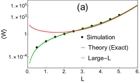
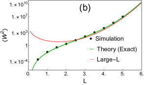
Figure 3: First two moments of the work done by the particle in presence of the harmonic potential $(n=2)$. In both panels, green curves are obtained by numerically differentiating the moment-generating function in Eq. (28), while red curves are the asymptotic results in Eqs. (31) and (32). We have chosen $v=k=D=1$.

We have verified these scaling behaviours in Figure 3 along with their exact counterparts.

Having looked at the first two moments, we next proceed to calculate the distribution of $W$. Obtaining the distribution using $Q(p,\xi_{0})$ in Eq. (28) analytically seems daunting. Nevertheless, in B we have provided a heuristic calculation that correctly gives the distribution for typical values of $W$ at large $L$. In particular, we find

$$P(W)\simeq\frac{2\exp\left(-\frac{\left\langle W\right\rangle}{2\left\langle W\right\rangle^{2}-\left\langle W^{2}\right\rangle}W\right)}{\sqrt{2\left\langle W^{2}\right\rangle-3\left\langle W\right\rangle^{2}}}~{}\sinh\left(\frac{\sqrt{2\left\langle W^{2}\right\rangle-3\left\langle W\right\rangle^{2}}}{2\left\langle W\right\rangle^{2}-\left\langle W^{2}\right\rangle}W\right),$$ (33)

as $L$ becomes large. We have compared this expression with the numerical simulations in Figure 4 and we observe an excellent match between them. For large $W$, the distribution decays exponentially as $\sim\exp\left(-W/\zeta_{W}\right)$ with the decay constant $\zeta_{W}=\frac{2\left\langle W\right\rangle^{2}-\left\langle W^{2}\right\rangle}{\left\langle W\right\rangle-\sqrt{2\left\langle W^{2}\right\rangle-3\left\langle W\right\rangle^{2}}}$. This is in stark contrast with the case of the fixed observation time, where distribution of $W$ for $n=2$ case just turns out to be a Gaussian function [69, 72]. In fact, the exponential decay turns out to be the hallmark property for the work distributions of all potentials with $n>1$ under a first-passage time as we discuss later.

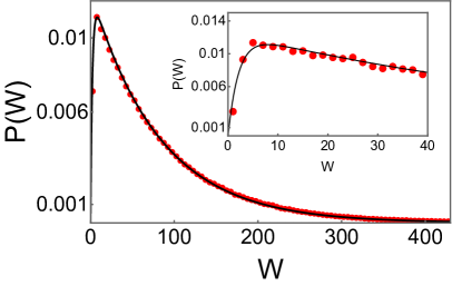
Figure 4: Probability distribution of the work done $W$ for the time-dependent harmonic potential $(n=2)$. Analytic expression in Eq. (33) is plotted in black and the simulation data are shown in red. Inset shows the comparison for small values of $W$. Parameters chosen are $v=k=D=1$, $L=4$.

5 General $n$

Having examined the analytically tractable cases, we now shift our focus to deriving general results applicable to arbitrary $n~{}(>0)$. While solving the backward equation (11) directly for a general $n$ is a challenging task, we can utilize it to derive a differential equation governing the moments of $W$, which we can subsequently solve. These moments can then be employed to deduce the behaviour of the distribution of $W$ for large $L$ as done for the linear and harmonic cases previously. Writing the $m$-th moment of $W$ as $\left\langle W^{m}(\xi_{0})\right\rangle=W_{m}(\xi_{0})$, we take the derivative with respect to $p$ in Eq. (11) to obtain

$$D\frac{d^{2}W_{m}(\xi_{0})}{d\xi_{0}^{2}}-\Big{(}kf_{n}(\xi_{0})+v\Big{)}\frac{dW_{m}(\xi_{0})}{d\xi_{0}}=mvkf_{n}(\xi_{0})W_{m-1}(\xi_{0}),$$ (34)

where $W_{0}(\xi_{0})=1$ and $f_{n}(\xi_{0})=\operatorname{sgn}(\xi_{0})\big{|}\xi_{0}\big{|}^{n-1}$. For $m=1$, the solution of this equation is given by

$$W_{1}\left(\xi_{0}\right) =\mathcal{B}+\mathcal{A}\operatorname{sgn}\left(\xi_{0}\right)\int_{0}^{\big{|}\xi_{0}\big{|}}dy~{}\mathcal{G}_{\operatorname{sgn}\left(\xi_{0}\right)}(y)+\operatorname{sgn}\left(\xi_{0}\right)\frac{kv}{D}\int_{0}^{\big{|}\xi_{0}\big{|}}dy~{}\mathcal{G}_{\operatorname{sgn}\left(\xi_{0}\right)}(y)\int_{0}^{y}dz~{}\frac{z^{n-1}}{\mathcal{G}_{\operatorname{sgn}\left(\xi_{0}\right)}(z)},$$

$$\text{with }\mathcal{G}_{\pm}(x)=\exp\left[\frac{1}{D}\left(\frac{kx^{n}}{n}\pm vx\right)\right],$$ (35)

and the constants $\mathcal{A}$ and $\mathcal{B}$ can be computed using the condition $W_{1}\left(\xi_{0}=\pm L\right)=0$. For $\xi_{0}=0$, the solution in Eq. (35) reduces to

$$\left\langle W\right\rangle=\frac{kv}{D}\frac{\left(\int_{0}^{L}dy~{}\mathcal{G}_{+}(y)\right)\left(\int_{0}^{L}dy~{}\mathcal{G}_{-}(y)\int_{0}^{y}dz~{}\frac{z^{n-1}}{\mathcal{G}_{-}(z)}\right)-\left(\int_{0}^{L}dy~{}\mathcal{G}_{-}(y)\right)\left(\int_{0}^{L}dy~{}\mathcal{G}_{+}(y)\int_{0}^{y}dz~{}\frac{z^{n-1}}{\mathcal{G}_{+}(z)}\right)}{\int_{0}^{L}dy~{}\left[\mathcal{G}_{+}(y)+\mathcal{G}_{-}(y)\right]}.$$ (36)

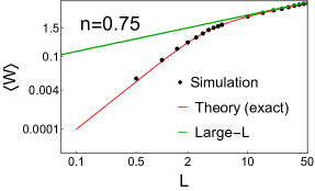
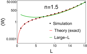
Figure 5: Illustration of the average work $\left\langle W\right\rangle$ performed by the particle in potentials with $n$ values $0.75$ and $1.5$. The theoretical plot is based on the expression in Eq. (36), presenting the exact calculation. In addition, the asymptotic large-$L$ results are given in Eq. (37). Parameters chosen are $k=0.5,~{}v=D=1$.

This is an exact expression of the mean valid for all $n$. Although analytically integrating in this expression turns out to be challenging in general, one can simplify the expression and obtain the leading order behaviour of $\left\langle W\right\rangle$ in the large-$L$ limit. As shown in C, this turns out to depend on the exponent $n$ and we get qualitatively different results depending on whether $n$ is greater or smaller than $1$. In particular, we have shown in C that

$$\left\langle W\right\rangle\sim\begin{cases}L^{1-n}~{}\exp\left[\frac{1}{D}\left(\frac{kL^{n}}{n}-vL\right)\right],~{}~{}~{}~{}~{}~{}\text{for }n>1,\\ L^{n},~{}~{}~{}~{}~{}~{}~{}~{}~{}~{}~{}~{}~{}~{}~{}~{}~{}~{}~{}~{}~{}~{}~{}~{}~{}~{}~{}~{}~{}~{}~{}~{}~{}~{}~{}~{}\text{for }n<1.\end{cases}$$ (37)

Let us now try to understand the difference between $n>1$ and $n<1$ cases physically. When the potential is sufficiently confining ($n>1$ case), the motion of the particle is heavily restricted due to the confining potential. Thus, typically the particle will be located away from the absorbing walls at $\pm L$ and it will hit them very rarely. Therefore, for $n>1$, the first-passage time to reach the walls is typically high which in turn gives large value for the work. On the other hand, for $n<1$, while the potential is still confining, the corresponding force decays with increasing distance. Hence, in Eq. (6), the drift $v$ term is always dominating beyond a certain distance. As a result, we get relatively smaller values of the first-passage time and hence the work.

In Figure 5, we have compared the exact result in Eq. (36) with the same obtained from the numerical simulations for $n<1$ (left panel) and $n>1$ (right panel). We observe an excellent agreement between the theory and the numerics for both cases. In addition to this, we have also presented a comparison of the large-$L$ expressions in Eq. (37) for the two cases. We find that Eq. (37) converges to the exact result as we take larger values of $L$.

So far in this section, we have solved Eq. (34) only for the mean $(m=1)$. But one can also utilize it to obtain the higher moments of $W$. A similar analysis for $m=2$ gives

$$\left\langle W^{2}\right\rangle=\frac{\left(\int_{0}^{L}dy~{}\mathcal{G}_{+}(y)\right)\left(\int_{0}^{L}dy~{}\mathcal{G}_{-}(y)\int_{0}^{y}dz~{}\frac{z^{n-1}W_{1}(-z)}{\mathcal{G}_{-}(z)}\right)-\left(\int_{0}^{L}dy~{}\mathcal{G}_{-}(y)\right)\left(\int_{0}^{L}dy~{}\mathcal{G}_{+}(y)\int_{0}^{y}dz~{}\frac{z^{n-1}W_{1}(z)}{\mathcal{G}_{+}(z)}\right)}{(2kv)^{-1}D\int_{0}^{L}dy~{}\left[\mathcal{G}_{+}(y)+\mathcal{G}_{-}(y)\right]}.$$ (38)

with the asymptotic behaviour derived in D to be

$$\left\langle W^{2}\right\rangle\simeq\begin{cases}2\left\langle W\right\rangle^{2},~{}~{}~{}~{}~{}~{}\text{for }n>1,\\ \left\langle W\right\rangle^{2},~{}~{}~{}~{}~{}~{}~{}~{}\text{for }n<1.\end{cases}$$ (39)

Note that these expressions only provide the leading order behaviour in $L$ and there are still sub-leading corrections that depend on model parameters $v$ and $k$. Interestingly, it turns out that one can use the first two moments to heuristically calculate the probability distribution describing the typical fluctuations of the work [as done before for $n=2$]. We refer to B for this calculation where we show

$$P(W)\simeq\frac{2\exp\left(-\frac{\left\langle W\right\rangle}{2\left\langle W\right\rangle^{2}-\left\langle W^{2}\right\rangle}W\right)}{\sqrt{2\left\langle W^{2}\right\rangle-3\left\langle W\right\rangle^{2}}}~{}\sinh\left(\frac{\sqrt{2\left\langle W^{2}\right\rangle-3\left\langle W\right\rangle^{2}}}{2\left\langle W\right\rangle^{2}-\left\langle W^{2}\right\rangle}W\right),~{}~{}~{}~{}~{}\text{for }n>1.$$ (40)

We emphasize that this expression only describes the typical fluctuations of $W$ around the mean for $n>1$ and will not capture the regimes far away from the mean. In Figure 6 (left panel), we have compared this with the numerics for $n=1.5$. We notice an excellent agreement between them. Next, we address the case where $n<1$. As observed in the instance of $n=1$ with $\gamma>0$, one needs to solve the complete backward equation (11) in order to obtain $Q(p,0)$. While achieving this for $n=1$ is feasible, doing the same analytically for arbitrary $n<1$ turns out to be difficult. However, based on extensive numerical simulation, we find that for $n<1$ also, the distribution has the same form (around the mean) as for $n=1$ with $\gamma>0$ in Eq. (23). This leads us to assume

$$P(W)\simeq\frac{1}{\sqrt{\mathbb{A}_{1}W^{3}}}~{}\exp\left[-\frac{\mathbb{A}_{2}}{W}\left(W-\mathbb{A}_{3}\right)^{2}\right],~{}~{}~{}~{}\text{for }n<1,$$ (41)

for large $L$. Here $\mathbb{A}_{1}$ and $\mathbb{A}_{2}$ and $\mathbb{A}_{3}$ are constants that depend on the parameters of the model. To compute them, we use the normalisation condition and the fact that the first two moments are given. We then obtain

$$\mathbb{A}_{1} =\frac{2\pi\left(\left\langle W^{2}\right\rangle-\left\langle W\right\rangle^{2}\right)}{\left\langle W\right\rangle^{3}},~{}~{}~{}\mathbb{A}_{2}=\frac{\left\langle W\right\rangle}{2\left[\left\langle W^{2}\right\rangle-\left\langle W\right\rangle^{2}\right]},~{}~{}~{}~{}\mathbb{A}_{3}=\left\langle W\right\rangle.$$ (42)

Plugging these constants in Eq. (41) gives

$$P(W)\simeq\sqrt{\frac{\left\langle W\right\rangle^{3}}{2\pi W^{3}\left(\left\langle W^{2}\right\rangle-\left\langle W\right\rangle^{2}\right)}}~{}\exp\left[-\frac{\left\langle W\right\rangle\left(W-\left\langle W\right\rangle\right)^{2}}{2W\left[\left\langle W^{2}\right\rangle-\left\langle W\right\rangle^{2}\right]}\right],~{}~{}~{}~{}\text{for }n<1.$$ (43)

The right panel in Figure 6 shows a comparison of Eq. (43) with the same obtained from the numerical simulations for $n=0.75$. An excellent match between them validates our results. In summary, we have derived the exact expressions for the first two moments and their large-$L$ forms in this section, applicable for all values of $n$. We then combined these expressions with a heuristic analysis to obtain the probability distribution of $W$ for large values of $L$ across all $n$ values.

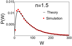
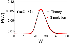
Figure 6: Comparison of the probability distribution of $W$ outlined in Eqs. (40) and (43) is presented in the left panel for $n>1$ and $L=10$ and the right panel for $n<1$ and $L=100$. We have set the parameters as $k=0.5$, $v=D=1$ for this comparison using numerical simulations.

6 Relation with the first-passage time

So far, we have studied the statistics of the work done till the particle reaches one of the walls at $L_{\pm}(t)$ for the first time. Deploying a backward approach in terms of the co-moving variable $\xi(t)$, we have been able to compute the first two moments and the probability distribution of $W$ for large $L$. In the remaining part of our paper, we show that the fluctuations of the work done $W$ bear an interesting relation with the fluctuations of the first-passage time $t_{f}$ defined in Eq. (4). In order to see this, we first write a backward equation for the moments $T_{m}(\xi_{0})=\left\langle t_{f}^{m}(\xi_{0})\right\rangle$ of the first-passage time as done before in Eq. (34) for the work done [51, 50]

$$D\frac{d^{2}T_{m}(\xi_{0})}{d\xi_{0}^{2}}-\Big{(}kf_{n}(\xi_{0})+v\Big{)}\frac{dT_{m}(\xi_{0})}{d\xi_{0}}=-mT_{m-1}(\xi_{0}),$$ (44)

where $T_{0}(\xi_{0})=1$ and $f_{n}(\xi_{0})=\operatorname{sgn}(\xi_{0})\big{|}\xi_{0}\big{|}^{n-1}$. Meanwhile the moments satisfy the boundary conditions $T_{m}\left(\xi_{0}=\pm L\right)=0$, since the particle gets instantly absorbed if its initial position coincides with one of the absorbing walls. Solving Eq. (44) in the same way as done in Section 5, we obtain for $m=1$

$$T_{1}\left(\xi_{0}\right) =\mathcal{B}_{1}+\mathcal{B}_{2}\operatorname{sgn}\left(\xi_{0}\right)\int_{0}^{\big{|}\xi_{0}\big{|}}dy~{}\mathcal{G}_{\operatorname{sgn}\left(\xi_{0}\right)}(y)-\frac{1}{D}\int_{0}^{\big{|}\xi_{0}\big{|}}dy~{}\mathcal{G}_{\operatorname{sgn}\left(\xi_{0}\right)}(y)\int_{0}^{y}\frac{dz}{\mathcal{G}_{\operatorname{sgn}\left(\xi_{0}\right)}(z)},$$ (45)

with functions $\mathcal{G}_{\pm}(y)$ given in Eq. (35). Constants $\mathcal{B}_{1}$ and $\mathcal{B}_{2}$ can be evaluated using the boundary conditions $T_{1}\left(\xi_{0}=\pm L\right)=0$. For $\xi_{0}=0$, the mean $\left\langle t_{f}\right\rangle=T_{1}(0)$ is given by

$$\left\langle t_{f}\right\rangle=\frac{1}{D}\frac{\left(\int_{0}^{L}dy~{}\mathcal{G}_{+}(y)\right)\left(\int_{0}^{L}dy~{}\mathcal{G}_{-}(y)\int_{0}^{y}\frac{dz}{\mathcal{G}_{-}(z)}\right)+\left(\int_{0}^{L}dy~{}\mathcal{G}_{-}(y)\right)\left(\int_{0}^{L}dy~{}\mathcal{G}_{+}(y)\int_{0}^{y}\frac{dz}{\mathcal{G}_{+}(z)}\right)}{\int_{0}^{L}dy~{}\left[\mathcal{G}_{+}(y)+\mathcal{G}_{-}(y)\right]},$$ (46)

For large $L$, the integrations in this expression can be approximately carried out as done for the work done. Proceeding similarly in C, we find

$$\left\langle t_{f}\right\rangle\sim\begin{cases}L^{1-n}~{}\exp\left[\frac{1}{D}\left(\frac{kL^{n}}{n}-vL\right)\right],~{}~{}~{}~{}~{}~{}\text{for }n>1,\\ L,~{}~{}~{}~{}~{}~{}~{}~{}~{}~{}~{}~{}~{}~{}~{}~{}~{}~{}~{}~{}~{}~{}~{}~{}~{}~{}~{}~{}~{}~{}~{}~{}~{}~{}~{}~{}~{}\text{for }n<1.\end{cases}$$ (47)

while for the marginal case of $n=1$, we obtain

$$\left\langle t_{f}\right\rangle\simeq\begin{cases}\frac{L}{\gamma D},~{}~{}~{}~{}~{}~{}~{}~{}~{}~{}~{}~{}~{}~{}~{}\text{for }\gamma>0,\\ \frac{L^{2}}{2D},~{}~{}~{}~{}~{}~{}~{}~{}~{}~{}~{}~{}~{}~{}~{}\text{for }\gamma=0,\\ \frac{2k}{\gamma^{2}D^{2}\mu}~{}e^{-\gamma L},~{}~{}~{}~{}\text{for }\gamma<0,\end{cases}~{}~{}~{}~{}(n=1).$$ (48)

Both Eqs. (47) and (48) give the leading order behaviours in $L$. Similarly, for $m=2$, one can solve Eq. (44) to show that the second moment $\left\langle t_{f}^{2}\right\rangle=\left\langle T_{m}(\xi_{0}=0)\right\rangle$ reads

$$\left\langle t_{f}^{2}\right\rangle=\frac{\left(\int_{0}^{L}dy~{}\mathcal{G}_{+}(y)\right)\left(\int_{0}^{L}dy~{}\mathcal{G}_{-}(y)\int_{0}^{y}dz~{}\frac{T_{1}(-z)}{\mathcal{G}_{-}(z)}\right)+\left(\int_{0}^{L}dy~{}\mathcal{G}_{-}(y)\right)\left(\int_{0}^{L}dy~{}\mathcal{G}_{+}(y)\int_{0}^{y}dz~{}\frac{T_{1}(z)}{\mathcal{G}_{+}(z)}\right)}{2^{-1}D\int_{0}^{L}dy~{}\left[\mathcal{G}_{+}(y)+\mathcal{G}_{-}(y)\right]}.$$ (49)

For large $L$, one can again simplify this expression [see D] and obtain

$$\left\langle t_{f}^{2}\right\rangle\simeq\begin{cases}2\left\langle t_{f}\right\rangle^{2},~{}~{}~{}~{}~{}~{}\text{for }n>1,\\ \left\langle t_{f}\right\rangle^{2},~{}~{}~{}~{}~{}~{}~{}~{}\text{for }n<1,\end{cases}$$ (50)

and for $n=1$, one gets

$$\left\langle t_{f}^{2}\right\rangle\simeq\begin{cases}\left\langle t_{f}\right\rangle^{2}+\frac{2L}{D^{2}\gamma^{3}},~{}~{}~{}~{}~{}~{}~{}~{}~{}\text{for }\gamma>0,\\ \frac{5L^{4}}{12D^{2}},~{}~{}~{}~{}~{}~{}~{}~{}~{}~{}~{}~{}~{}~{}~{}~{}~{}~{}~{}\text{for }\gamma=0,\\ 2\left\langle t_{f}\right\rangle^{2},~{}~{}~{}~{}~{}~{}~{}~{}~{}~{}~{}~{}~{}~{}~{}~{}\text{for }\gamma<0.\end{cases}~{}~{}~{}~{}(n=1).$$ (51)

Once again in Eq. (50), we only obtain the leading order asymptotic expression in $L$. However, there will be sub-leading corrections that depend on parameters $v$ and $k$ and we do not delve into these corrections in Eq. (50).

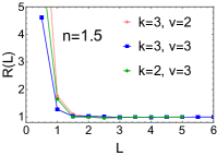
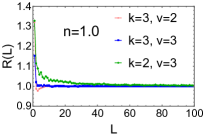
Figure 7: Simulation results for the ratio $R(L)$ defined in Eq. (53) for three cases of $n>1$, $n=1$ and $n<1$. For every $n$, we have considered scenarios with $v<k$ (pink), $v=k$ (blue) and $v>k$ (green).

Next to see the connection of the first-passage time with the work done, we define their coefficents of variation as

$$\text{CV}\big{|}_{W}=\sqrt{\frac{\left\langle W^{2}\right\rangle-\left\langle W\right\rangle^{2}}{\left\langle W\right\rangle^{2}}},~{}~{}~{}~{}\text{and }~{}~{}~{}\text{CV}\big{|}_{t_{f}}=\sqrt{\frac{\left\langle t_{f}^{2}\right\rangle-\left\langle t_{f}\right\rangle^{2}}{\left\langle t_{f}\right\rangle^{2}}},$$ (52)

and then look at the following ratio

$$R(L)=\left(\frac{\text{CV}\big{|}_{W}}{\text{CV}\big{|}_{t_{f}}}\right)^{2}.$$ (53)

For $n=1$, one can plug the analytic expressions of first and second moments of $W$ and $t_{f}$ derived in the previous sections and show that the ratio $R(L)$ converges to the value $1$ as the length $L$ becomes large for all values of $v$ and $k$. Similarly, for $n>1$, one can use the asymptotic results $\left\langle W^{2}\right\rangle\simeq 2\left\langle W\right\rangle^{2}$ and $\left\langle t_{f}^{2}\right\rangle\simeq 2\left\langle t_{f}\right\rangle^{2}$ to show that both $\text{CV}\big{|}_{W}$ and $\text{CV}\big{|}_{t_{f}}$ individually go to $1$. This indicates that the ratio $R(L)$ also converges to $1$ for larger $L$ for $n>1$. However for $n<1$, an analytical calculation of $R(L)$ remains unlikely. As indicated in Eqs. (39) and (50), for the case of $n<1$, one needs to have the knowledge of the sub-leading corrections in $L$ within the expressions of $\langle W^{2}\rangle$ and $\langle t_{f}^{2}\rangle$ in order to compute the $CV$-s. Moreover, extracting these corrections analytically from the exact expression turns out to be difficult and our analysis in Eqs. (39) and (50) cannot capture these details. In Figure 7, we have plotted the ratio $R(L)$ as a function of the initial wall separation $L$ for different values of the exponent $n$. For $n\geq 1$, we find that $R(L)$ indeed saturates to the universal value equal to one at large $L$ independent of the model parameters $k$, $v$ and $D$. On the other hand, for $n<1$, the large-$L$ behaviour of $R(L)$ depends on these parameters. For instance, in Figure 7 [right panel], we see that the saturation values for $v=3,~{}k=3$ (shown in blue) and $v=3,~{}k=2$ (shown in green) are completely different for $n=0.8$. On the other hand, for $v=2,~{}k=3$ (shown in pink), $R(L)$ increases monotonically at large $L$ and does not saturate to a constant value. This is possibly due to the fact that the saturation of $R(L)$ only takes place at large $L$, i.e. for $L\gg L_{\text{th}}$, where $L_{\text{th}}$ is some threshold length. For a given $n$, the threshold $L_{\text{th}}$ also depends on the parameters $v$ and $k$. In Figure 7 [right panel], we find that $L_{\text{th}}\sim 50$ for the green curve $\left(k/v<1\right)$ whereas $L_{\text{th}}\sim 500$ for the blue one $\left(k/v=1\right)$. Thus, we see a consistent rise in the value of $L_{\text{th}}$ as the ratio $k/v$ starts to increase. Following this trend, we anticipate $L_{\text{th}}$ to be very large for the pink curve $\left(k/v>1\right)$. Probing such large $L$ values in simulations is computationally expensive. Thus, we observe that $R(L)$ increases for the pink curve since we are still in the regime $L\ll L_{\text{th}}$. However, if we go to very large $L$ values (beyond what is considered in the figure), we anticipate $R(L)$ to converge to a constant value even for the pink curve $(v=2,~{}k=3)$.

7 Conclusion

In summary, we have analyzed the work statistics in a driven overdamped system in one dimension. In contrast to the conventional cases where the observables are usually measured upto a fixed time, here we measure the work upto a random first passage time that is conditioned on a certain criterion. We employ the Feynman-Kac path integral approach to compute the work functional in various set-ups consisting of potentials of different configurations. We provide a comprehensive analysis of the work fluctuations which shows a rich behavior as a function of the potential strength, the external drive and the interval over which the particle moves. Furthermore, we showed an interesting symmetry relation between the signal-to-noise relation or the variability of the work and that of the first-passage time. To understand this phenomena better, we also delved deeper into the attributing physical conditions. Notably, our results illustrate a marked difference in the work statistics between systems driven up to a fixed time and a first-passage time.

Moving forward, it would be interesting to study the generality of the “variability relation” in other systems and to identify any unifying physics behind it. There has been a myriad of studies in recent times in the field of stochastic thermodynamics involving various other thermodynamic observables such as injected power, dissipated heat or entropy production. It is only natural to study the same also within our set-up and will be pursued elsewhere. Furthermore, our model could also be useful to study existing thermodynamic bounds for first-passage-time problems [73, 24, 41, 37]. Concluding, we believe that our results can be tested using optical trap experiments [72, 74, 75] which may unfold another layer of interesting observations.

Appendix A Large-$L$ behaviour of $Q(p,0)$ for the linear potential

In this appendix, we provide the derivation of the simplified expression of the moment generating function $Q(p,0)$ for large $L$ as written in Eq. (22). For this, we first rewrite the exact expression of $Q(p,0)$ in Eq. (19) as,

$$Q(p,0)=\frac{\mathcal{N}(p)}{\mathcal{D}(p)},$$ (54)

where the functions $\mathcal{N}(p)$ and $\mathcal{D}(p)$ are given by

$$\mathcal{N}(p) =\left[\lambda_{+}(p)-\lambda_{-}(p)\right]\left[e^{-\sigma_{+}(p)L}-e^{-\sigma_{-}(p)L}\right]+\left[\sigma_{+}(p)-\sigma_{-}(p)\right]\left[e^{\lambda_{-}(p)L}-e^{\lambda_{+}(p)L}\right],$$ (55)

$$\mathcal{D}(p) =\left[\lambda_{-}(p)-\sigma_{+}(p)\right]e^{\left[\lambda_{+}(p)-\sigma_{-}(p)\right]L}+\left[\sigma_{+}(p)-\lambda_{+}(p)\right]e^{\left[\lambda_{-}(p)-\sigma_{-}(p)\right]L}$$

$$~{}~{}~{}~{}~{}~{}~{}~{}~{}~{}~{}~{}~{}~{}+\left[\lambda_{+}(p)-\sigma_{-}(p)\right]e^{\left[\lambda_{-}(p)-\sigma_{+}(p)\right]L}+\left[\sigma_{-}(p)-\lambda_{-}(p)\right]e^{\left[\lambda_{+}(p)-\sigma_{+}(p)\right]L},$$ (56)

with $\lambda_{\pm}(p)$ and $\sigma_{\pm}(p)$ given in Eq (17). In order to simplify this expression further, we first note that the work done by the particle typically attains a large positive value which scales either algebraically or exponentially with the length $L$, as seen from the expression of $\left\langle W\right\rangle$ in Eq. (21). In terms of $p$-variable, this translates to taking the $p\to 0$ limit in $Q(p,0)$. However, for small $p$, the leading order form of $Q(p,0)$ crucially depends on the signature of $\gamma$. Below we consider these different cases separately.

A.1 $\gamma>0$ case

For $p\to 0$ limit, we find that $\sigma_{+}(p)\simeq\gamma$, $\lambda_{+}(p)\simeq\mu$, whereas both $\sigma_{-}(p)$ and $\lambda_{-}(p)$ are of order $\sim p$. Therefore, we find that $\mathcal{N}(p)\simeq-\gamma e^{\mu L}$ and $\mathcal{D}(p)\simeq-\gamma e^{\left[\mu-\sigma_{-}(p)\right]L}$. Plugging this in Eq. (54), we find

$$Q(p,0)\simeq\exp\left[\sigma_{-}(p)L\right],~{}~{}~{}~{}~{}\text{for }\gamma>0.$$ (57)

A.2 $\gamma<0$ case

On the other hand, for $\gamma<0$, we find $\sigma_{-}(p)\simeq\gamma$, $\lambda_{+}(p)\simeq\mu$, while both $\sigma_{+}(p)$ and $\lambda_{-}(p)$ are linear order in $p$. This implies that to the leading order, we have

$$\mathcal{N}(p) \simeq\left[\sigma_{-}(p)-\sigma_{+}(p)\right]e^{\lambda_{+}(p)L},$$ (58)

$$\mathcal{D}(p) \simeq e^{\lambda_{+}(p)L}\left[e^{-\sigma_{+}(p)L}\Big{(}\sigma_{-}(p)-\lambda_{-}(p)\Big{)}+e^{-\sigma_{-}(p)L}\Big{(}\lambda_{-}(p)-\sigma_{+}(p)\Big{)}\right].$$ (59)

Inserting these expressions in Eq. (54) and performing the small $p$ expansion further, we obtain

$$Q(p,0)\simeq\left[1+p\left\langle W\right\rangle\left(1+\frac{kvL}{D\big{|}\gamma\big{|}}p\right)\right]^{-1},~{}~{}~{}~{}\text{for }\gamma<0.$$ (60)

A.3 $\gamma=0$ case

For this case, we have $\lambda_{+}(p)\simeq\mu$, $\lambda_{-}(p)\simeq v^{2}p/\mu D$ and $\sigma_{\pm}(p)=\pm\sqrt{v^{2}p/D}$. Plugging this in Eq. (54) and performing the small $\lambda_{-}$ expansion we find

$$Q(p,0)\simeq\frac{\mu\left\{\exp(2\alpha L\sqrt{p})-1\right\}+2\beta\sqrt{p}\exp(\alpha L\sqrt{p})}{\mu\left\{\exp(2\alpha L\sqrt{p})-1\right\}+\beta\sqrt{p}~{}\left\{\exp(2\alpha L\sqrt{p})+1\right\}},~{}~{}~{}~{}~{}~{}\text{for }\gamma=0.$$ (61)

Appendix B Heuristic derivation of the distribution $P(W)$ for $n>1$

In this appendix, we will give a hand-waving derivation of the distribution of the work done in Eq. (40) for $n>1$. To begin with, we first recall that for large $L$, the work done typically attains large positive values as indicated by Eq. (37). In terms of the moment generating function $Q(p,0)$, this corresponds to performing a small $p$ approximation. Indeed, for the case of linear potential, this led us to obtain a simplified expression of $Q(p,0)$ in Eq. (22). In fact, for all $n>1$, we find that the moment-generating function can be expressed as

$$Q(p,0) \simeq 1-p\left\langle W\right\rangle+\frac{\left\langle W^{2}\right\rangle}{2}p^{2},$$ (62)

$$\simeq\left[1+p\left\langle W\right\rangle+p^{2}\left(\left\langle W\right\rangle^{2}-\frac{\left\langle W^{2}\right\rangle}{2}\right)\right]^{-1},$$ (63)

for large $L$ with moments $\left\langle W\right\rangle$ and $\left\langle W^{2}\right\rangle$ given in Eqs. (36) and (38) respectively. Performing the inverse Laplace transformation, we then obtain

$$P(W)\simeq\frac{2\exp\left(-\frac{\left\langle W\right\rangle}{2\left\langle W\right\rangle^{2}-\left\langle W^{2}\right\rangle}W\right)}{\sqrt{2\left\langle W^{2}\right\rangle-3\left\langle W\right\rangle^{2}}}~{}\sinh\left(\frac{\sqrt{2\left\langle W^{2}\right\rangle-3\left\langle W\right\rangle^{2}}}{2\left\langle W\right\rangle^{2}-\left\langle W^{2}\right\rangle}W\right),~{}~{}~{}~{}~{}\text{for }n>1.$$ (64)

This expression has been presented in Eq. (40) in the main text.

Appendix C Asymptotic behaviour of the mean work for large $L$

Here, we derive the simplified expression of the mean work $\left\langle W\right\rangle$ for large $L$. The exact expression was derived in Eq. (36) which we rewrite here as

$$\left\langle W\right\rangle=\frac{kv}{D}\frac{\mathcal{J}_{+}(L)~{}\mathcal{I}_{-}(L)-\mathcal{J}_{-}(L)~{}\mathcal{I}_{+}(L)}{\mathcal{J}_{+}(L)+\mathcal{J}_{-}(L)},$$ (65)

with $$\mathcal{J}_{\pm}(L)=\int_{0}^{L}dy~{}\mathcal{G}_{\pm}(y),~{}~{}\text{and}~{}~{}\mathcal{I}_{\pm}(L)=\int_{0}^{L}dy~{}\mathcal{G}_{\pm}(y)\int_{0}^{y}dz~{}\frac{z^{n-1}}{\mathcal{G}_{\pm}(z)},$$ (66)

where $\mathcal{G}_{\pm}(y)$ are given in Eq. (35). In order to find the large-$L$ behaviour of $\left\langle W\right\rangle$, we have to calculate the corresponding forms of the functions $\mathcal{J}_{\pm}(L)$ and $\mathcal{I}_{\pm}(L)$. These however turn out to depend on the exponent $n$ and we get different forms depending on whether $n$ is greater or smaller than $1$. Below we consider these two cases separately.

C.1 $n>1$ case

For $n>1$, both $\mathcal{G}_{\pm}(y)$ functions have faster than exponential growth for large argument. This indicates that both $\mathcal{J}_{\pm}(L)$ also grow with $L$. To see this, we write them as

$$\mathcal{J}_{\pm}(L) =\int_{0}^{L}dy~{}\exp\left[\frac{1}{D}\left(\frac{ky^{n}}{n}\pm vy\right)\right],$$ (67)

$$=L\int_{0}^{1}d\omega~{}\exp\left[\frac{1}{D}\left(\frac{k\omega^{n}L^{n}}{n}\pm v\omega L\right)\right],~{}~{}~{}~{}(\omega=y/L).$$ (68)

For large $L$, the integrand has a maximum value at $\omega=1$. Moreover, this value increases with $L$. Therefore, for large $L$, the overall integration in Eq. (68) will get major contribution from the vicinity of $\omega=1$. Performing an expansion of the integrand in Eq. (68) around $y=1-u$ and keeping the leading order in $u$, we get the large-$L$ behaviour of $\mathcal{J}_{\pm}(L)$ as

$$\mathcal{J}_{\pm}(L) \sim L~{}\exp\left[\frac{1}{D}\left(\frac{kL^{n}}{n}\pm vL\right)\right]\times\int_{0}^{1}du~{}\exp\left[-\frac{u}{D}\left(kL^{n}\pm vL\right)\right],$$ (69)

$$\sim L^{1-n}~{}\exp\left[\frac{1}{D}\left(\frac{kL^{n}}{n}\pm vL\right)\right].$$ (70)

We next turn to $\mathcal{I}_{\pm}(L)$. Rewriting their forms from Eq. (66)

$$\mathcal{I}_{\pm}(L) =\int_{0}^{L}dy~{}~{}\exp\left[\frac{1}{D}\left(\frac{ky^{n}}{n}\pm vy\right)\right]\int_{0}^{y}dz~{}z^{n-1}\exp\left[-\frac{1}{D}\left(\frac{kz^{n}}{n}\pm vz\right)\right],$$ (71)

$$=L\int_{0}^{1}d\omega~{}\exp\left[\frac{1}{D}\left(\frac{k\omega^{n}L^{n}}{n}\pm v\omega L\right)\right]~{}\int_{0}^{\omega L}dz~{}z^{n-1}\exp\left[-\frac{1}{D}\left(\frac{kz^{n}}{n}\pm vz\right)\right].$$ (72)

Let us first analyse the integration over $z$ for large values of $L$. By Changing the variable $u=kz^{n}/nD$, this integral can be rewritten as

$$\int_{0}^{\omega L}dz~{}z^{n-1} \exp\left[-\frac{1}{D}\left(\frac{kz^{n}}{n}\pm vz\right)\right]$$ (73)

$$\sim\int_{0}^{\frac{kw^{n}L^{n}}{nD}}du~{}e^{-u}\sum_{i=0}^{\infty}\left(\mp\frac{v}{D}\right)^{i}~{}\left(\frac{Dn}{k}\right)^{\frac{i}{n}}\frac{u^{\frac{i}{n}}}{i!},$$ (74)

$$\sim\sum_{i=0}^{\infty}\left(\mp\frac{v}{D}\right)^{i}~{}\left(\frac{Dn}{k}\right)^{\frac{i}{n}}\frac{\Gamma\left(1+i/n\right)}{i!},~{}~{}~{}~{}~{}~{}~{}~{}\text{as }L\to\infty.$$ (75)

The sum converges for $n>1$. This implies that the integration over $z$ in Eq. (72) becomes independent of $wL$ as $L$ becomes very large (for a given $\omega$) and $\mathcal{I}_{\pm}(L)$ accordingly takes the form

$$\mathcal{I}_{\pm}(L) \sim L\int_{0}^{1}d\omega~{}\exp\left[\frac{1}{D}\left(\frac{k\omega^{n}L^{n}}{n}\pm v\omega L\right)\right],$$ (76)

$$\sim L^{1-n}~{}\exp\left[\frac{1}{D}\left(\frac{kL^{n}}{n}\pm vL\right)\right],$$ (77)

where the second line follows from Eq. (70). Combining this result with the expressions of $\mathcal{J}_{\pm}(L)$ in Eq. (70) and plugging all of them in Eq. (65), we find

$$\left\langle W\right\rangle\sim L^{1-n}~{}\exp\left[\frac{1}{D}\left(\frac{kL^{n}}{n}-vL\right)\right],~{}~{}~{}~{}\text{for }n>1\text{ and large }L.$$ (78)

C.2 $n<1$ case

Let us now derive the large-$L$ expression of the mean work $\left\langle W\right\rangle$ for $n<1$. Looking at Eq. (65), this again translates to calculating the functions $\mathcal{J}_{\pm}(L)$ and $\mathcal{I}_{\pm}(L)$. We first notice that even for $n<1$, $\mathcal{G}_{+}(y)$ has a faster than exponential growth for large $y$. Therefore, one can follow a similar approach as described in Section C.1 for $\mathcal{J}_{+}(L)$ and $\mathcal{I}_{+}(L)$ and obtain

$$\begin{cases}&\mathcal{J}_{+}(L)\sim\exp\left[\frac{1}{D}\left(\frac{kL^{n}}{n}+vL\right)\right],\\ &\mathcal{I}_{+}(L)\sim\exp\left[\frac{1}{D}\left(\frac{kL^{n}}{n}+vL\right)\right],\end{cases}~{}~{}~{}~{}~{}(\text{for large }L).$$ (79)

On the other hand, $\mathcal{G}_{-}(y)$ for $n<1$ is a decaying function for large $y$ and requires a different approach. To this end, we recast $\mathcal{J}_{-}(L)$ as

$$\mathcal{J}_{-}(L)=\int_{0}^{L}dy~{}e^{-vy/D}~{}\sum_{i=0}^{\infty}\left(\frac{k}{nD}\right)^{i}\frac{y^{ni}}{i!},$$ (80)

and carry out the integration over $y$ for $L\to\infty$ to yield

$$\mathcal{J}_{-}(L)\sim\sum_{i=0}^{\infty}\left(\frac{k}{D^{1-n}n~{}v^{n}}\right)^{i}~{}\frac{\Gamma\left(1+ni\right)}{i!}.$$ (81)

For $n<1$, this is a convergent sum. Hence $\mathcal{J}_{-}(L)$ becomes independent of $L$ for this case. Next we turn to $\mathcal{I}_{-}(L)$ whose explicit expression follows from Eq. (66) as

$$\mathcal{I}_{-}(L)=\int_{0}^{L}dy~{}~{}\exp\left[-\frac{1}{D}\left(vy-\frac{ky^{n}}{n}\right)\right]\int_{0}^{y}dz~{}z^{n-1}\exp\left[\frac{1}{D}\left(vz-\frac{kz^{n}}{n}\right)\right].$$ (82)

By changing the variables $y=\omega L$ and $z=u\omega L$, this expression becomes

$$\mathcal{I}_{-}(L)=L^{n+1}\int_{0}^{1}d\omega~{}\omega^{n}\exp\left[-\frac{\omega L}{D}\left(v-\frac{k}{n\left(\omega L\right)^{1-n}}\right)\right]\int_{0}^{1}du~{}u^{n-1}~{}\exp\left[\frac{u\omega L}{D}\left(v-\frac{k}{n\left(u\omega L\right)^{1-n}}\right)\right].$$

For large $L$ and fixed $\omega$ and $u$, one can simplify this expression as

$$\mathcal{I}_{-}(L) \simeq L^{n+1}\int_{0}^{1}d\omega~{}\omega^{n}\exp\left[-\frac{v\omega L}{D}\right]\int_{0}^{1}du~{}u^{n-1}~{}\exp\left[\frac{vu\omega L}{D}\right],$$ (83)

$$\simeq L^{n+1}\int_{0}^{1}d\omega~{}\omega^{n}\exp\left(-\frac{v\omega L}{D}\right)~{}\left(-\frac{D}{v\omega L}\right)^{n}\left[\Gamma\left(n\right)-\Gamma\left(n,-\frac{v\omega L}{D}\right)\right].$$ (84)

Using the approximate form of the gamma function as $\Gamma\left(n,-x\right)\stackrel{{\scriptstyle x\to\infty}}{{~{}\simeq~{}}}(-x)^{n-1}~{}e^{x}$ and then performing the integration over $\omega$ gives

$$\mathcal{I}_{-}(L)\simeq\frac{D}{nv}L^{n},~{}~{}~{}\text{for large }L.$$ (85)

Finally, using this result along with the results derived in Eqs. (79) and (81) and inserting all of them in Eq. (66), we obtain the large-$L$ behaviour of the mean work as

$$\left\langle W\right\rangle\simeq\frac{kv}{D}~{}\mathcal{I}_{-}(L)\sim L^{n},~{}~{}~{}~{}\text{for }n<1.$$ (86)

Eqs. (78) and (86) have been quoted in Eq. (37) in the main text.

Appendix D Variance of the work done for large $L$

In this appendix, we will derive the simplified leading-order expression for the variance $\left\langle W^{2}\right\rangle$ of the work done for large $L$. The starting point is the exact expression in Eq. (38) which we rewrite as

$$\left\langle W^{2}\right\rangle=\frac{2kv}{D}~{}\frac{\mathcal{J}_{+}(L)~{}\mathcal{Y}_{-}(L)-\mathcal{J}_{-}(L)~{}\mathcal{Y}_{+}(L)}{\mathcal{J}_{+}(L)+\mathcal{J}_{-}(L)},$$ (87)

where $\mathcal{J}_{\pm}(L)$ are given in Eq. (66) and functions $\mathcal{Y}_{\pm}(L)$ are

$$\mathcal{Y}_{\pm}(L)=\int_{0}^{L}dy~{}\mathcal{G}_{\pm}(y)\int_{0}^{y}dz~{}W_{1}(\pm z)~{}\frac{z^{n-1}}{\mathcal{G}_{\pm}(z)},$$ (88)

with $\mathcal{G}_{\pm}(y)$ defined in Eq. (35). In order to find the large-$L$ expression of $\left\langle W^{2}\right\rangle$, we have to calculate the corresponding form of these functions. Meanwhile, we computed $\mathcal{J}_{\pm}(L)$ in C and showed that they take different forms depending on whether the exponent $n$ is greater than or smaller than one. In the following, we carry out the same analysis for $\mathcal{Y}_{\pm}(L)$.

D.1 $n>1$ case

Let us write the explicit expression of $\mathcal{Y}_{\pm}(L)$

$$\mathcal{Y}_{\pm}(L) =\int_{0}^{L}dy~{}~{}\exp\left[\frac{1}{D}\left(\frac{ky^{n}}{n}\pm vy\right)\right]\int_{0}^{y}dz~{}z^{n-1}~{}W_{1}(\pm z)~{}\exp\left[-\frac{1}{D}\left(\frac{kz^{n}}{n}\pm vz\right)\right].$$ (89)

Looking at this, we first notice that for $y$ integration, the integrand has a faster than exponential growth. This implies that at large $L$, this integration will be dominated predominantly by the larger values of $y$. On the other hand, the integration over $z$ is damped due to the presence of the decaying exponential term. Therefore, even though $y$ takes larger values, the integration over $z$ will still be dominated by small values of $z$ (more precisely $z\ll L$). This allows us to replace $W_{1}(\pm z)\simeq W_{1}(0)$ in Eq. (89) and recast it as

$$\mathcal{Y}_{\pm}(L)\simeq W_{1}(0)~{}\mathcal{I}_{\pm}(L),$$ (90)

where $\mathcal{I}_{\pm}(L)$ are given in Eq. (66). Inserting this in Eq. (87) then yields

$$\left\langle W^{2}\right\rangle\simeq\frac{2kv\left\langle W\right\rangle}{D}\frac{\mathcal{J}_{+}(L)~{}\mathcal{I}_{-}(L)-\mathcal{J}_{-}(L)~{}\mathcal{I}_{+}(L)}{\mathcal{J}_{+}(L)+\mathcal{J}_{-}(L)},$$ (91)

after which we use Eq. (65) to obtain

$$\left\langle W^{2}\right\rangle\simeq 2\left\langle W\right\rangle^{2},~{}~{}~{}~{}\text{for large }L.$$ (92)

D.2 $n<1$ case

We now turn to the other case of $n<1$. First recall that in C.2, we showed that the functions $\mathcal{J}_{\pm}(L)$ for this case scale as

$$\begin{cases}&\mathcal{J}_{+}(L)\sim\exp\left[\frac{1}{D}\left(\frac{kL^{n}}{n}+vL\right)\right],\\ &\mathcal{J}_{-}(L)\sim\text{independent of }L,\end{cases}~{}~{}~{}~{}~{}(\text{for large }L).$$ (93)

Similarly, for $\mathcal{Y}_{+}(L)$, we notice that $\mathcal{G}_{+}(y)$ is a growing function in $y$ even for $n<1$. This indicates that the approximations used in deriving Eq. (90) for $\mathcal{Y}_{+}(L)$ will remain valid also for $n<1$ and we have

$$\mathcal{Y}_{+}(L)\sim L^{n}~{}\exp\left[\frac{1}{D}\left(\frac{kL^{n}}{n}+vL\right)\right].$$ (94)

However $\mathcal{Y}_{-}(L)$ has to be treated in a different way since $\mathcal{G}_{-}(y)$ is now a decaying function at large $y$. To this end, we first change the variables $y=\omega L$ and $z=u\omega L$ in Eq. (88) and rewrite it as

$$\mathcal{Y}_{-}(L)= L^{n+1}\int_{0}^{1}d\omega~{}\omega^{n}\exp\left[-\frac{\omega L}{D}\left(v-\frac{k}{n\left(\omega L\right)^{1-n}}\right)\right]$$

$$~{}~{}~{}~{}~{}~{}~{}~{}\times\int_{0}^{1}du~{}u^{n-1}~{}W_{1}(-u\omega L)\exp\left[\frac{u\omega L}{D}\left(v-\frac{k}{n\left(u\omega L\right)^{1-n}}\right)\right].$$ (95)

Taking large $L$ limit for fixed $\omega$ and $u$, this simplifies to

$$\mathcal{Y}_{-}(L)\simeq L^{n+1}\int_{0}^{1}d\omega~{}\omega^{n}\exp\left[-\frac{v\omega L}{D}\right]\int_{0}^{1}du~{}u^{n-1}~{}~{}W_{1}(-u\omega L)~{}\exp\left[\frac{vu\omega L}{D}\right].$$ (96)

This expression is similar to Eq. (83) except for the presence of $W_{1}(-u\omega L)$ term. In D.3, we show that

$$W_{1}(-u\omega L)\simeq\left\langle W\right\rangle(1-\omega^{n}u^{n}),~{}~{}~{}~{}\text{for large }L.$$ (97)

Plugging this expression in Eq. (96) and performing the approximations as done in Eq. (83) yields

$$\mathcal{Y}_{-}(L)\simeq\frac{\left\langle W\right\rangle}{2}~{}\mathcal{I}_{-}(L).$$ (98)

Recall that both $\left\langle W\right\rangle$ and $\mathcal{I}_{-}(L)$ scale as $\sim L^{n}$ for large $L$ [see Eq. (86)] which implies that $\mathcal{Y}_{-}(L)\sim L^{2n}$.

We now have all functions needed to compute $\left\langle W^{2}\right\rangle$ in Eq. (87). Inserting the functions $\mathcal{J}_{\pm}(L)$ and $\mathcal{Y}_{\pm}(L)$ from Eqs. (93), (94) and (98) in Eq. (87), we finally obtain for $n<1$

$$\left\langle W^{2}\right\rangle \simeq\frac{kv\left\langle W\right\rangle}{D}~{}\mathcal{I}_{-}(L),$$ (99)

$$\simeq\left\langle W\right\rangle^{2},~{}~{}\text{[using Eq.~{}\eqref{apeen-mean-work-eq-13}]}.$$ (100)

D.3 Proof of Eq. (97)

In the remaining part of this section, we provide a derivation of Eq. (97) which was instrumental in deriving $\left\langle W^{2}\right\rangle$ for $n<1$ case. Following Eq. (35), we can write the mean work as

$$W_{1}(-u\omega L)=\left\langle W\right\rangle-\mathcal{A}~{}\mathcal{J}_{-}(u\omega L)-\frac{kv}{D}~{}\mathcal{I}_{-}(u\omega L).$$ (101)

For $n<1$, $J_{-}(u\omega L)$ is independent of $L$ as indicated in Eq. (93) whereas $I_{-}(u\omega L)$ scales as $\sim u^{n}\omega^{n}L^{n}$ [shown in Eq. (85)]. Using this in Eq. (101), we obtain

$$W_{1}(-u\omega L) \simeq\left\langle W\right\rangle-\frac{k}{n}u^{n}\omega^{n}L^{n},$$ (102)

$$\simeq\left\langle W\right\rangle\left(1-u^{n}\omega^{n}\right).$$ (103)

This proved the result in Eq. (97).

References

References

- [1] Seifert U 2012 Reports on Progress in Physics 75 126001 URL https://dx.doi.org/10.1088/0034-4885/75/12/126001
- [2] Van den Broeck C and Esposito M 2015 Physica A: Statistical Mechanics and its Applications 418 6–16 URL https://www.sciencedirect.com/science/article/pii/S037843711400346X
- [3] Peliti L and Pigolotti S 2021 Stochastic Thermodynamics: An Introduction (Princeton University Press) ISBN 978-0691201771
- [4] Sekimoto K 1998 Progress of Theoretical Physics Supplement 130 17–27 URL https://doi.org/10.1143/PTPS.130.17
- [5] Seifert U 2005 Phys. Rev. Lett. 95(4) 040602 URL https://link.aps.org/doi/10.1103/PhysRevLett.95.040602
- [6] Crooks G E 1999 Phys. Rev. E 60(3) 2721–2726 URL https://link.aps.org/doi/10.1103/PhysRevE.60.2721
- [7] Crooks G E 2000 Phys. Rev. E 61(3) 2361–2366 URL https://link.aps.org/doi/10.1103/PhysRevE.61.2361
- [8] Hayashi K, Ueno H, Iino R and Noji H 2010 Phys. Rev. Lett. 104(21) 218103 URL https://link.aps.org/doi/10.1103/PhysRevLett.104.218103
- [9] Jarzynski C 1997 Phys. Rev. Lett. 78(14) 2690–2693 URL https://link.aps.org/doi/10.1103/PhysRevLett.78.2690
- [10] Evans D J and Searles D J 1994 Phys. Rev. E 50(2) 1645–1648 URL https://link.aps.org/doi/10.1103/PhysRevE.50.1645
- [11] Gallavotti G and Cohen E 1995 Journal of Statistical Physics 80 931–970 URL https://doi.org/10.1007/BF02179860
- [12] Gupta D, Plata C A and Pal A 2020 Physical review letters 124 110608
- [13] Barato A C and Seifert U 2015 Phys. Rev. Lett. 114(15) 158101 URL https://link.aps.org/doi/10.1103/PhysRevLett.114.158101
- [14] Gingrich T R, Horowitz J M, Perunov N and England J L 2016 Phys. Rev. Lett. 116(12) 120601 URL https://link.aps.org/doi/10.1103/PhysRevLett.116.120601
- [15] Proesmans K and den Broeck C V 2017 Europhysics Letters 119 20001 URL https://dx.doi.org/10.1209/0295-5075/119/20001
- [16] Hasegawa Y and Van Vu T 2019 Phys. Rev. Lett. 123(11) 110602 URL https://link.aps.org/doi/10.1103/PhysRevLett.123.110602
- [17] Timpanaro A M, Guarnieri G, Goold J and Landi G T 2019 Phys. Rev. Lett. 123(9) 090604 URL https://link.aps.org/doi/10.1103/PhysRevLett.123.090604
- [18] Koyuk T and Seifert U 2019 Phys. Rev. Lett. 122(23) 230601 URL https://link.aps.org/doi/10.1103/PhysRevLett.122.230601
- [19] Proesmans K and Horowitz J M 2019 Journal of Statistical Mechanics: Theory and Experiment 2019 054005 URL https://dx.doi.org/10.1088/1742-5468/ab14da
- [20] Harunari P E, Fiore C E and Proesmans K 2020 Journal of Physics A: Mathematical and Theoretical 53 374001 URL https://dx.doi.org/10.1088/1751-8121/aba05e
- [21] Pal S, Saryal S, Segal D, Mahesh T S and Agarwalla B K 2020 Phys. Rev. Res. 2(2) 022044 URL https://link.aps.org/doi/10.1103/PhysRevResearch.2.022044
- [22] Pal A, Reuveni S and Rahav S 2021 Phys. Rev. Res. 3(1) 013273 URL https://link.aps.org/doi/10.1103/PhysRevResearch.3.013273
- [23] Pal A, Reuveni S and Rahav S 2021 Phys. Rev. Res. 3(3) L032034 URL https://link.aps.org/doi/10.1103/PhysRevResearch.3.L032034
- [24] Falasco G and Esposito M 2020 Phys. Rev. Lett. 125(12) 120604 URL https://link.aps.org/doi/10.1103/PhysRevLett.125.120604
- [25] Kuznets-Speck B and Limmer D T 2021 Proceedings of the National Academy of Sciences 118 e2020863118 URL https://www.pnas.org/doi/abs/10.1073/pnas.2020863118
- [26] Yan L L, Zhang J W, Yun M R, Li J C, Ding G Y, Wei J F, Bu J T, Wang B, Chen L, Su S L, Zhou F, Jia Y, Liang E J and Feng M 2022 Phys. Rev. Lett. 128(5) 050603 URL https://link.aps.org/doi/10.1103/PhysRevLett.128.050603
- [27] Shiraishi N, Funo K and Saito K 2018 Phys. Rev. Lett. 121(7) 070601 URL https://link.aps.org/doi/10.1103/PhysRevLett.121.070601
- [28] Aurell E, Mejía-Monasterio C and Muratore-Ginanneschi P 2011 Phys. Rev. Lett. 106(25) 250601 URL https://link.aps.org/doi/10.1103/PhysRevLett.106.250601
- [29] Ito S and Dechant A 2020 Phys. Rev. X 10(2) 021056 URL https://link.aps.org/doi/10.1103/PhysRevX.10.021056
- [30] Aurell E, Gawȩdzki K, Mejía-Monasterio C, Mohayaee R and Muratore-Ginanneschi P 2012 Journal of Statistical Physics 147 487–505 URL https://doi.org/10.1007/s10955-012-0478-x
- [31] Zhen Y Z, Egloff D, Modi K and Dahlsten O 2021 Phys. Rev. Lett. 127(19) 190602 URL https://link.aps.org/doi/10.1103/PhysRevLett.127.190602
- [32] Sivak D A and Crooks G E 2012 Phys. Rev. Lett. 108(19) 190602 URL https://link.aps.org/doi/10.1103/PhysRevLett.108.190602
- [33] Proesmans K, Ehrich J and Bechhoefer J 2020 Phys. Rev. Lett. 125(10) 100602 URL https://link.aps.org/doi/10.1103/PhysRevLett.125.100602
- [34] Proesmans K, Ehrich J and Bechhoefer J 2020 Phys. Rev. E 102(3) 032105 URL https://link.aps.org/doi/10.1103/PhysRevE.102.032105
- [35] Van Vu T and Saito K 2022 Phys. Rev. Lett. 128(1) 010602 URL https://link.aps.org/doi/10.1103/PhysRevLett.128.010602
- [36] Dechant A 2022 Journal of Physics A: Mathematical and Theoretical 55 094001 URL https://dx.doi.org/10.1088/1751-8121/ac4ac0
- [37] Neri I, Roldán E and Jülicher F 2017 Phys. Rev. X 7(1) 011019 URL https://link.aps.org/doi/10.1103/PhysRevX.7.011019
- [38] Chétrite R, Gupta S, Neri I and Roldán E 2019 Europhysics Letters 124 60006 URL https://dx.doi.org/10.1209/0295-5075/124/60006
- [39] Manzano G, Fazio R and Roldán E 2019 Phys. Rev. Lett. 122(22) 220602 URL https://link.aps.org/doi/10.1103/PhysRevLett.122.220602
- [40] Neri I, Roldán E, Pigolotti S and Jülicher F 2019 Journal of Statistical Mechanics: Theory and Experiment 2019 104006 URL https://dx.doi.org/10.1088/1742-5468/ab40a0
- [41] Neri I 2020 Phys. Rev. Lett. 124(4) 040601 URL https://link.aps.org/doi/10.1103/PhysRevLett.124.040601
- [42] Chétrite R and Gupta S 2011 Journal of Statistical Physics 143 543–584 URL https://doi.org/10.1007/s10955-011-0184-0
- [43] Neri I 2022 SciPost Phys. 12 139 URL https://scipost.org/10.21468/SciPostPhys.12.4.139
- [44] Roldán E, Neri I, Dörpinghaus M, Meyr H and Jülicher F 2015 Phys. Rev. Lett. 115(25) 250602 URL https://link.aps.org/doi/10.1103/PhysRevLett.115.250602
- [45] Neri I 2022 Journal of Physics A: Mathematical and Theoretical 55 304005 URL https://dx.doi.org/10.1088/1751-8121/ac736b
- [46] Singh S, Menczel P, Golubev D S, Khaymovich I M, Peltonen J T, Flindt C, Saito K, Roldán E and Pekola J P 2019 Phys. Rev. Lett. 122(23) 230602 URL https://link.aps.org/doi/10.1103/PhysRevLett.122.230602
- [47] Manzano G and Roldán E 2022 Phys. Rev. E 105(2) 024112 URL https://link.aps.org/doi/10.1103/PhysRevE.105.024112
- [48] Neri I and Polettini M 2023 SciPost Phys. 14 131 URL https://scipost.org/10.21468/SciPostPhys.14.5.131
- [49] Roldán E, Neri I, Chétrite R, Gupta S, Pigolotti S, Jülicher F and Sekimoto K 2023 (Preprint arXiv:2210.09983) URL https://doi.org/10.48550/arXiv.2210.09983
- [50] Majumdar S N 2005 Current Science 89 93–129 URL https://www.worldscientific.com/doi/abs/10.1142/9789812772718_0006
- [51] Kac M 1949 Transactions of the American Mathematical Society 65 1–13 URL http://www.jstor.org/stable/1990512
- [52] Kearney M J 2004 Journal of Physics A: Mathematical and General 37 8421 URL https://dx.doi.org/10.1088/0305-4470/37/35/002
- [53] Dhar D and Ramaswamy R 1989 Phys. Rev. Lett. 63(16) 1659–1662 URL https://link.aps.org/doi/10.1103/PhysRevLett.63.1659
- [54] Prellberg T and Brak R 1995 Journal of Statistical Physics 78 701–730
- [55] Dean D S and Majumdar S N 2001 Journal of Physics A: Mathematical and General 34 L697 URL https://dx.doi.org/10.1088/0305-4470/34/49/102
- [56] Richard C 2002 Journal of Statistical Physics 108 459–493
- [57] Majumdar S N and Kearney M J 2007 Phys. Rev. E 76(3) 031130 URL https://link.aps.org/doi/10.1103/PhysRevE.76.031130
- [58] Alan J Bray S N M and Schehr G 2013 Advances in Physics 62 225–361 URL https://doi.org/10.1080/00018732.2013.803819
- [59] Abundo M 2013 Methodology and Computing in Applied Probability 15 85–103
- [60] Kearney M J and Majumdar S N 2005 Journal of Physics A: Mathematical and General 38 4097 URL https://dx.doi.org/10.1088/0305-4470/38/19/004
- [61] Majumdar S N and Meerson B 2020 Journal of Statistical Mechanics: Theory and Experiment 2020 023202 URL https://dx.doi.org/10.1088/1742-5468/ab6844
- [62] Abundo M and Vescovo D 2017 Methodology and Computing in Applied Probability 19 985–996
- [63] Meerson B 2023 Phys. Rev. E 107(6) 064122 URL https://link.aps.org/doi/10.1103/PhysRevE.107.064122
- [64] Abundo M and Furia S 2019 Methodology and Computing in Applied Probability 21 1283–1302
- [65] Kearney M J and Martin R J 2021 Journal of Physics A: Mathematical and Theoretical 54 055002 URL https://dx.doi.org/10.1088/1751-8121/abd677
- [66] Abundo M 2021 Stochastic Analysis and Applications 41 358–376 URL https://doi.org/10.1080/07362994.2021.2018335
- [67] Singh P and Pal A 2022 Journal of Physics A: Mathematical and Theoretical 55 234001 URL https://dx.doi.org/10.1088/1751-8121/ac677c
- [68] Dubey A and Pal A 2023 Journal of Physics A: Mathematical and Theoretical 56 435002 URL https://dx.doi.org/10.1088/1751-8121/acf748
- [69] van Zon R and Cohen E G D 2003 Phys. Rev. E 67(4) 046102 URL https://link.aps.org/doi/10.1103/PhysRevE.67.046102
- [70] van Zon R and Cohen E G D 2003 Phys. Rev. Lett. 91(11) 110601 URL https://link.aps.org/doi/10.1103/PhysRevLett.91.110601
- [71] Mazonka O and Jarzynski C 1999 (Preprint arXiv:cond-mat/9912121) URL https://doi.org/10.48550/arXiv.cond-mat/9912121
- [72] Ciliberto S 2017 Physical Review X 7 021051
- [73] Gingrich T R and Horowitz J M 2017 Physical review letters 119 170601
- [74] Proesmans K, Dreher Y, Gavrilov M, Bechhoefer J and Van den Broeck C 2016 Physical Review X 6 041010
- [75] Nalupurackal G, Lokesh M, Suresh S, Roy S, Chakraborty S, Goswami J, Pal A and Roy B New Journal of Physics