Linear stability and spectral modal decomposition of three-dimensional turbulent wake flow of a generic high-speed train

Abstract

This work investigates the spatio-temporal evolution of coherent structures in the wake of a generic high-speed train, based on a three-dimensional database from large eddy simulation. Spectral proper orthogonal decomposition is used to extract energy spectra and energy ranked empirical modes for both symmetric and antisymmetric components of the fluctuating flow field. The spectrum of the symmetric component shows overall higher energy and more pronounced low-rank behavior compared to the antisymmetric one, with the most dominant symmetric mode at $\omega=3.437$ characterized by vortex shedding in the near wake and constant streamwise wavenumber structures in the far wake. The mode bispectrum further reveals the dominant role of self-interaction of the symmetric component, leading to first harmonic and subharmonic triads of the fundamental frequency, with remarkable deformation of the mean field. Then, the stability of the three dimensional wake flow is analyzed based on two-dimensional local linear stability analysis. Temporal stability analysis is first performed for both the near wake and the far wake regions, showing a more unstable condition in the near wake region. The absolute frequency of the near-wake eigenmode is determined based on spatio-temporal analysis, then tracked along the streamwise direction to find out the global mode growth rate and frequency, which indicate a marginally stable global mode oscillating at a frequency very close to the most dominant SPOD mode. The global mode wavemaker is then located, and the structural sensitivity is calculated based on the direct and adjoint modes derived from a local spatial analysis, with the maximum value localized within the recirculation region close to the train tail. Finally, the global mode shape is computed by tracking the most spatially unstable eigenmode in the far wake, and the alignment with the SPOD mode is computed as a function of streamwise location. By combining data-driven and theoretical approaches, the mechanisms of coherent structures in complex wake flows are well identified and isolated.

1 Introduction

In the face of climate change, high-speed rail has gradually developed to become the key to decarbonizing transportation. As a bluff body operating at high Reynolds number ($\mathit{Re}$), the flow around a high-speed train exhibits complex characteristics of a fully developed three-dimensional turbulent flow (Schetz, 2001). The unsteady aerodynamics of high-speed trains is then directly characterized by the fluctuating aerodynamic forces and induced slipstreams. Therefore, understanding the dominant dynamics in the complex turbulent flow around the train is crucial to improving and optimizing aerodynamic performance. For this purpose, the search for and identification of physically significant coherent structures, or modes, is a suitable method (Taira et al., 2017). In fact, extracting and understanding the physical mechanisms of instability in complex three-dimensional turbulent flow has been attracting research interest for several decades but remains challenging. In particular, the complexity of the base flow, as well as the high demand for computational resources, causes huge difficulties in solving this problem (Theofilis, 2011). However, due to the increasing demand for transportation efficiency, passenger comfort, and operational safety, extracting and understanding the mechanisms of instability in the flow around the train is still of great research interest and significant engineering importance.

Despite its aerodynamic design, the high-speed train exhibits bluff-body flow characteristics reminiscent of those of the well-studied Ahmed body (Ahmed et al., 1984; Lienhart et al., 2002). Three important structures can be identified in the wake of the body: a recirculation bubble over the slanted surface, a pair of longitudinal C-pillar vortices generated from the two side edges of the slanted surface, and a recirculation zone behind the rear vertical base. Several studies have focused on the interaction and control strategies of these structures. In Zhang et al. (2015); Liu et al. (2021), the unsteady characteristics of Ahmed bodies in the high- and low-drag regimes were investigated using multiple experimental techniques. On the basis of these findings, several steady blow drag reduction strategies have been successfully developed Zhang et al. (2018); Li et al. (2022). Meanwhile, random switching between two reflectional-symmetry breaking states of the wake has been investigated in Grandemange et al. (2013); He et al. (2021a), with appropriate strategies altering the natural bi-stability of the wake proposed in Grandemange et al. (2014); Evstafyeva et al. (2017); Haffner et al. (2020).

However, the full picture of the three-dimensional coherent structures in the wake, as well as the associated instability information, remains limited. Therefore, further interpretation and understanding of the physical mechanisms that generate disturbances in the flow are limited. In particular, for more aerodynamically shaped high-speed trains, the identification of the flow structures mentioned above is less obvious. To extend understanding and control of wake dynamics in a more complex situation, modal decomposition (Taira et al., 2017) of the three-dimensional flow must be taken into consideration, which is the objective of this work.

Data-driven analysis has proven to be an effective method to extract coherent structures from flow snapshots as empirical modes. The most classic and widely used data-driven approach, proper orthogonal decomposition (POD), was first introduced to the field of fluid dynamics by Lumley (1967, 1970). In this approach, the flow is represented as a mean and a superposition of space-time-dependent modes. These resulting modes can then be used for a variety of purposes, from classification to reduced order modeling to control (Rowley & Dawson, 2017; Taira et al., 2017). Meanwhile, many other empirical approaches have been proposed. For example, the Balanced POD (Rowley, 2005) which serves as an expansion for linear input-output relationships, and Dynamic Mode Decomposition (DMD) (Schmid, 2010) which approximates the dynamics of a higher-order system through a combination of linearly growing or decaying modes.

In this paper, we focus on the application of the spectral form of POD, which is called spectral proper orthogonal decomposition (SPOD). This method is derived from the space-time formulation of POD for statistically stationary flow. The resulting modes, which oscillate at a single frequency, are orthogonal under a space-time inner product. In general, SPOD combines the advantages of the classical POD and DMD for statistically stationary flows, meanwhile, it provides an improved robustness over these two methods Towne et al. (2018). Furthermore, this method has been further extended to achieve more features, such as frequency-time (Nekkanti & Schmidt, 2021) and triadic interaction Schmidt (2020) analysis, or better convergence (Blanco et al., 2022; Schmidt, 2022) and lower computational cost (Schmidt & Towne, 2019), and therefore has received increasing interest in identifying coherent turbulent structures that are physically meaningful in various flow problems. These applications include jet (Schmidt et al., 2018), pipe flow (Abreu et al., 2020), flow around airfoils (Abreu et al., 2021), disk wake (Nidhan et al., 2022), and various industrial flows (Haffner et al., 2020; He et al., 2021b; Li et al., 2021a; Wang et al., 2022b).

Considering vehicle wake flow, coherent structures represented by empirical modes are within the research scope of several studies listed above (He et al., 2021a; Grandemange et al., 2013; Haffner et al., 2020; Li et al., 2021a). However, these applications are limited to two-dimensional planes in the wake, which do not fully capture the complex three-dimensional space-time coherent structures in the flow. Therefore, this study further extends the previous results shown in Li et al. (2021a) where a parameter study using a two-dimensional database from train wake flow is performed, to find coherent structures from a global perspective. However, although SPOD extracts modes related to the dominant fluctuation of the flow, this method is purely data-driven and model-free. As such, it does not reveal the mechanisms driving the coherent structures. However, it includes all non-linear dynamics and may reveal interactions between the structures in a quantitative manner. To further search for the instability mechanisms, one may use either stochastic low order dynamic models (Rigas et al., 2015; Sieber et al., 2021) or a mean field stability analysis.

Mean field linear stability analysis is considered to provide further insight into the mechanisms driving the flow dynamics. It is known that a self-excited oscillation can be described by an unstable global mode (Chomaz, 2005) derived from a global stability analysis. Recently, improved feasibility of large-scale linear algebra computations enables tri-global stability analysis of flows with three inhomogeneous directions (Theofilis, 2011). Some applications include boundary layer flows with isolated roughness elements (Loiseau et al., 2014; Kurz & Kloker, 2016; Ma & Mahesh, 2022), lid-driven cavity flows (Paredes, 2014; Gómez et al., 2014), jets in crossflow (Regan & Mahesh, 2017), and wakes of rectangular prisms (Zampogna & Boujo, 2023). When mean flows display homogeneity in the direction normal to convective motion, the Bi-Global stability approach can be utilized. This approach considers two-dimensional modes with a spatial wavenumber in the third dimension, and has been applied to a broad range of canonical flow Theofilis (2003, 2011), as well as complex technical flows including swirling flows (Kaiser et al., 2018; Müller et al., 2020), reacting flows (Casel et al., 2022; Wang et al., 2022a), turbo-machinery flows (Müller et al., 2022) and two-phase flows (Schmidt & Oberleithner, 2023). For mean flows weakly evolving in the convection direction, either the tri-global or bi-global method can be applied locally, i.e. local one-dimensional analysis in the lines normal to the streamwise direction to construct bi-global instability. As reviewed by Huerre & Monkewitz (1990), the method is based on a spatio-temporal analysis of the local velocity profile invoking the WKBJ approximation. The relationship between local absolute instability and global modes can be found in Monkewitz et al. (1993); Chomaz (2005), which concluded that a region of local absolute instability is a necessary condition for the existence of global instability. Comparisons between results of local and global stability analysis can be found in Giannetti & Luchini (2007); Juniper et al. (2011); Juniper & Pier (2015); Kaiser et al. (2018); Demange et al. (2022). In general, local stability analyses require less computational memory than global stability analyzes, since they convert a large matrix eigenvalue problem into several small independent matrix eigenvalue problems (Juniper & Pier, 2015). Meanwhile, as the local linearized Navier-Stokes equation is solved at each discrete streamwise position, the eigenvalues can be continuously tracked to provide an accurate spatial description of the mode. Therefore, local stability analysis is still widely used for flows beyond the range of global analysis (Pier, 2008; Oberleithner et al., 2011; Rukes et al., 2016).

To the best of the author’s knowledge, there are limited studies regarding the linear instability mechanisms of fully developed turbulent wake flows behind vehicles. Zampogna & Boujo (2023) investigated the global stability of rectangular prisms with rounded front edges, which approximate the geometry of the Ahmed body. However, this study considered a laminar flow without ground effect, such that the problem could be treated with two symmetries. From a more practical perspective, flows behind high-speed trains may consist of a series of vortex structures that are subject only to a spanwise symmetry condition. In addition, the spatial and temporal evolution of these vortex structures differs greatly from free-evolving structures due to the presence of the ground (Schetz, 2001). Up to now, the instability mechanisms in typical vehicle wakes of high industrial relevance remain an unanswered question. Is there a linear global mode that drives the instability in the turbulent wake? How does the linear global mode compare to the leading SPOD mode? Which part of the wake serves as the origin of the global instability and is most sensitive to external forcing? These questions need to be answered to serve as a basis for further optimizations, while extending the applications of these two approaches to more complex flow problems and higher $\mathit{Re}$.

Since the flow problem considered is only subject to spanwise symmetry, the tri-global stability with three inhomogeneous directions should be considered. The WKBJ approximation then converts the three-dimensional linearized problem into several two-dimensional local problems to account for global instability. This is generally a more complex situation than the research shown in Juniper & Pier (2015); Rukes et al. (2016); Kaiser et al. (2018), where local one-dimensional analyzes are used to construct the bi-global mode. Meanwhile, the parallelism or weak non-parallelism in local analysis could be a strong assumption (Chomaz, 2005; Pier, 2008; Rukes et al., 2016; Puckert & Rist, 2018) in the flow problem considered. How nonparallelism would affect the results of global instability and how to deal with nonparallelism in the complex base flow are also important issues to be solved.

The outline of the paper is as follows. The large eddy simulation setup used to obtain the three-dimensional flow field around the train is shown in $\S$2, along with the description of the time-averaged wake-flow structures. In $\S$3, we use SPOD to extract the dominant empirical modes and provide a first insight into the spatio-temporal characteristic of the coherent structures. Meanwhile, bispectral mode decomposition is considered to compute frequency triads, which explains the features in the SPOD spectrum. The tri-global stability mode obtained from two-dimensional local stability analysis is presented in $\S$4. In $\S$5, we compare the SPOD mode with the linear global mode at each streamwise location, and the mechanism of the fundamental instability is interpreted based on the comparison results. The main findings and conclusions are summarized in $\S$6.

2 Flow problem description

2.1 Large Eddy Simulation

The database for both the data-driven and theoretical mode calculations is obtained from a large eddy simulation performed with the commercial code STAR-CCM+ 14.02. A complete description of the numerical setup and validation can be found in Li et al. (2021b), here only the essential information is presented.

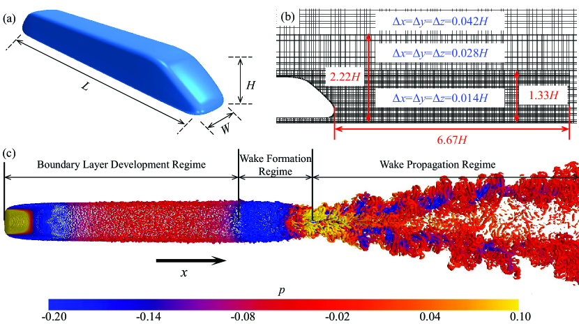
Figure 1: Large Eddy Simulation setup. (a) Geometric model; (b) Distribution of computational grid; (c) Instantaneous snapshot of vortex structures.

A simplified version of the Intercity-Express 2 (ICE2), also known as the aerodynamic train model (ATM), is considered. The simulation is carried out on the scale of 1:10, resulting in the height of the model $H=0.36m$, the width of the model $W=0.30m$ and the length of the model $L=2.5m$, as shown in figure 1(a). To simulate the relative motion between the train and the surrounding environment, the upstream boundary, located 10$H$ from the train head, is assigned the inflow velocity $U_{\infty}$. Meanwhile, the ground boundary, with a distance to the train bottom surface of 0.15$H$, is defined with the same moving velocity. The resulting $\mathit{Re}$ based on the height of the train and $U_{\infty}$ is $9.5\times 10^{4}$. The downstream boundary is located 30$H$ from the train tail, with a zero static pressure outlet condition. On the side and roof of the computational domain, the symmetry plane boundary condition is assigned, with a distance of 10$H$ from the train model. The computational domain is then discretized using unstructured hexahedral volume meshes, with the wall normal and wall parallel distances expressed in viscous units, respectively ${\Delta}y^{+}=0.16$ and ${\Delta}x^{+}={\Delta}z^{+}=28$ for cells attached to the train surface, as shown in figure 1(b). The total number of volume meshes used in the study is 46.8 million.

In the current research, the large eddy simulation based on the wall-adapting local-eddy viscosity (WALE) subgrid-scale model is chosen. The use of a novel form of the velocity gradient tensor in the WALE subgrid scale model allows for much more universal model coefficients compared to other widely used subgrid scale models. Meanwhile, the WALE subgrid scale model does not require any form of near-wall damping but automatically provides accurate scaling at the walls. More details about the WALE subgrid scale model can be found in Nicoud & Ducros (1999). An implicit unsteady segregated incompressible finite-volume solver is used, with the convective terms discretized based on a bounded central-differencing scheme, and the diffusion and turbulence terms are discretized with the second-order upstream scheme. The time marching procedure is performed using the implicit second-order accurate three-time level scheme, with the discretized convective time step set to $0.0067t^{*}$ ($t^{*}=W/U_{\infty}$), which leads to the Courant-Friedrichs-Lewy number below unity in most of the computational grids. The simulation was first run for $66.7t^{*}$ in order to reach a statistically stationary state, and then was run for a duration of $800t^{*}$ to collect field data. An instantaneous scene of the flow structures around the generic high-speed train, which briefly illustrates the formation of the turbulent wake, is shown in 1(c).

The three-dimensional snapshot database is continuously collected from a square box extending from $x/W=-1.33$ upstream of the tail nose tip to $x/W=6.67$ downstream of the tail nose tip, $y/W=1.33$ from the center plane of the train in both spanwise directions, and $z/W=1.33$ from the ground in the vertical direction. The time step between two consecutive snapshots is $0.1t^{*}$, resulting in a total of 8000 snapshots collected during the simulation. These values have been shown to be sufficient to produce well-converged SPOD results according to the parametric study shown in Li et al. (2021a).

2.2 Mean flow properties

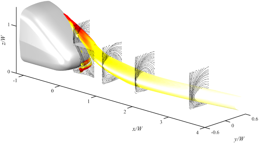
Figure 2: Time-averaged mean flow structures visualized by iso-surface of vortex identification criterion $\Omega=0.6$ and streamlines.

We consider the time-averaged field as the base state for the linear stability analysis and introduce it in this section. Furthermore, prior knowledge of the mean field will facilitate understanding of the physics associated with the extracted coherent structures. In figure 2, the time-averaged sectional streamlines are shown at several representative locations. Meanwhile, vortex regions are identified by the isosurface of $\Omega$ (Liu et al., 2016), colored by the magnitude of the vorticity. The $\Omega$-method works as a vortex identification criterion similar to the $Q$-criterion and ${\lambda}_{2}$-criterion, however, it is less sensitive to threshold value to capture both strong and weak vortices in different cases. Note that the wake flow is symmetric about the central plane after long-term time averaging, so only the $y>0$ half is shown here for better visualization.

It can be observed that, the attached flow on the slanted and bottom surfaces of the tail propagates downstream and approaches the rear end. Then, the strong adverse pressure near the tail nose point forces the attached flow particles to separate from the train surfaces, forming the spanwise vortex pair located just behind the tail nose point. Meanwhile, in addition to the flow structures related to the separation near the rear end, we can also observe the longitudinal vortex located above the side edge of the slanted surface of the tail, which is similar in nature to the C-pillar vortex in the Ahmed body wake flow Zhang et al. (2015); Liu et al. (2021); He et al. (2021a); Li et al. (2022). This pair of longitudinal vortex is formed by flow separation from the side surface, which exerts a strong pressure-suction effect in this area and continuously rolls up flow particles from the slanted surface. As the longitudinal vortex propagates downstream, it gradually increases in diameter and lifts away from the tail surface, moving toward the ground along the tail side edge. Due to the strong downwash from the slanted surface, the trailing vortex can be observed to move away from the central symmetry plane as it travels downstream. At $x/W\approx 1.5$, the longitudinal vortex structure attaches to the ground and then propagates nearly parallel to the ground in the downstream wake. In general, the mean field is fully three-dimensional in the near wake region, and its complexity gradually decreases downstream of the solid body, developing to be nearly parallel downstream of $x/W\approx 2.0$. The two main features, the spanwise recirculation bubble and the streamwise vortex pair, should be related to the mean field instability due to the strong velocity gradient and will therefore be discussed further in the following content.

3 Data-driven coherent structure identification

3.1 Symmetric & antisymmetric decomposition

Based on the spanwise symmetry of the described flow problem, fluctuations of the sampled flow field can be divided into symmetric and antisymmetric contributions (Hack & Schmidt, 2021). To properly isolate coherent structures defined by the two different types of fluctuations, an additive decomposition was applied to the collected snapshot data before extracting empirical modes. Defining the fluctuating part of the flow field as

$$\mathbf{q}^{\prime}(t)=\mathbf{q}(t)-\bar{\mathbf{q}}=\begin{bmatrix}u(x,y,z,t)-\bar{u}(x,y,z)\\ v(x,y,z,t)-\bar{v}(x,y,z)\\ w(x,y,z,t)-\bar{w}(x,y,z)\\ p(x,y,z,t)-\bar{p}(x,y,z)\end{bmatrix}=\begin{bmatrix}u^{\prime}(x,y,z,t)\\ v^{\prime}(x,y,z,t)\\ w^{\prime}(x,y,z,t)\\ p^{\prime}(x,y,z,t)\end{bmatrix}$$ (1)

where $\bar{\left(.\right)}$ denotes the time-averaged flow quantities and $\left(.\right)^{\prime}$ is the fluctuating part. Then, the spanwise symmetric and antisymmetric contributions can be obtained using the following expression.

$$\mathbf{q}^{\prime}_{S}(t)=\frac{1}{2}\begin{bmatrix}u^{\prime}(x,y,z,t)+u^{\prime}(x,-y,z,t)\\ v^{\prime}(x,y,z,t)-v^{\prime}(x,-y,z,t)\\ w^{\prime}(x,y,z,t)+w^{\prime}(x,-y,z,t)\\ p^{\prime}(x,y,z,t)+p^{\prime}(x,-y,z,t)\end{bmatrix}$$ (2)

$$\mathbf{q}^{\prime}_{A}(t)=\frac{1}{2}\begin{bmatrix}u^{\prime}(x,y,z,t)-u^{\prime}(x,-y,z,t)\\ v^{\prime}(x,y,z,t)+v^{\prime}(x,-y,z,t)\\ w^{\prime}(x,y,z,t)-w^{\prime}(x,-y,z,t)\\ p^{\prime}(x,y,z,t)-p^{\prime}(x,-y,z,t)\end{bmatrix}$$ (3)

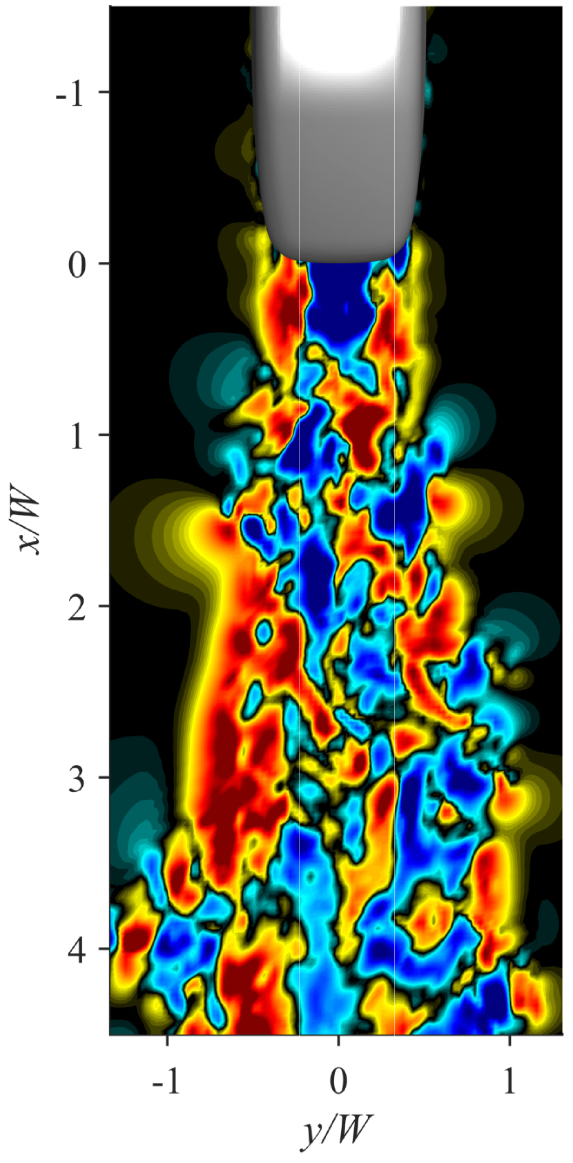
a

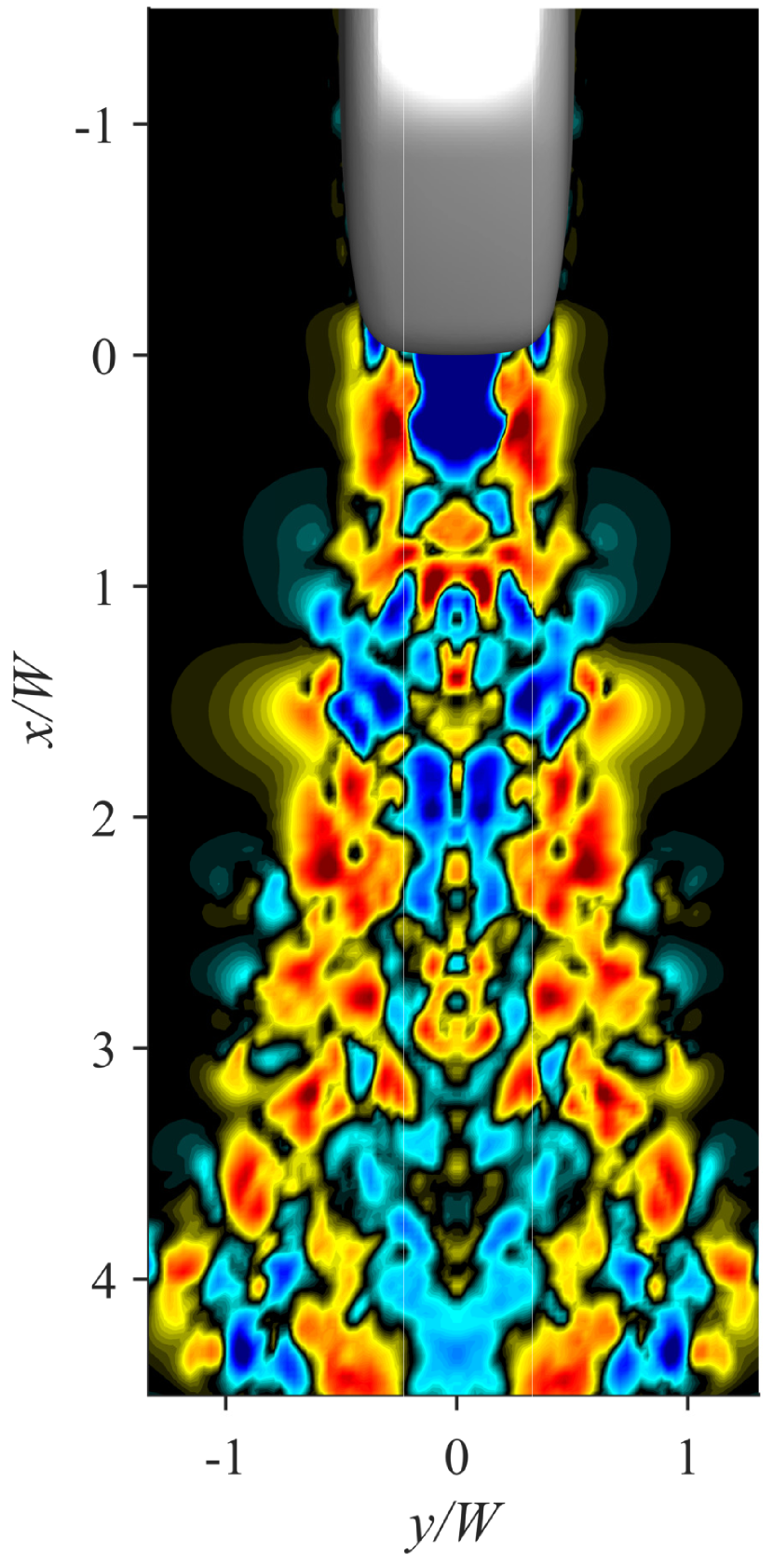
b

c

Figure 3: Symmetric & antisymmetric decomposition on instantaneous snapshot. (a) Original field; (b) Symmetric component; (c) antisymmetric component.

A visualization of one snapshot of the fluctuating streamwise velocity field, together with the contributions from the symmetric and antisymmetric components, is shown in figure 3.

The spanwise symmetrical and anti-symmetrical contributions of all collected samples are arranged into two separate data matrices as

$$\mathbf{Q}_{S} =\begin{bmatrix}\mathbf{q}^{\prime}_{S,1}&\mathbf{q}^{\prime}_{S,2}&...&\mathbf{q}^{\prime}_{S,n_{\rm{t}}}\end{bmatrix}$$ (4a)

$$\mathbf{Q}_{A} =\begin{bmatrix}\mathbf{q}^{\prime}_{A,1}&\mathbf{q}^{\prime}_{A,2}&...&\mathbf{q}^{\prime}_{A,n_{\rm{t}}}\end{bmatrix}$$ (4b)

The two independent data matrices then serve as the basis for extracting and analyzing, respectively, the symmetric and antisymmetric empirical modes. Note that, due to the zero-integral property of an even and an odd function in the sampling domain, the symmetric and antisymmetric modes yield mutual orthogonality (Hack & Schmidt, 2021).

3.2 Spectral proper orthogonal decomposition

The SPOD approach seeks modes that are optimal in terms of the space-time inner product defined as

$$\int_{-\infty}^{\infty}\int_{\Omega}\mathbf{q}^{H}(\mathbf{x},t)\mathbf{q}(\mathbf{x},t){\rm{d}}\mathbf{x}{\rm{d}}t$$ (5)

where the superscript $\left(.\right)^{H}$ denotes the Hermitian transpose. This problem is solved with SPOD by extending the database to the frequency domain, and searching for spatially orthogonal basis at each discrete frequency, following the standard POD routine. The derived modes can then optimally represent space-time flow statistics (Schmidt et al., 2018; Towne et al., 2018).

To do this, the snapshot database is first segmented into $n_{\rm{blk}}$ overlapping blocks, with $n_{\rm{DFT}}$ snapshots in each individual block. Note that to avoid zero padding in the discrete Fourier transform, $n_{\rm{DFT}}=256$ is used in our study, and the resulting angular frequency resolution is 0.245. An overlap of $50\%$ is used, as a larger overlap number does not improve the spectral estimation results (Schmidt & Colonius, 2020). With the above parameters, $n_{\rm{blk}}$ can be determined with the value of 61, which is sufficient for well-converged SPOD energy spectrum and modes (Schmidt & Colonius, 2020). Along with an appropriate window function, a discrete Fourier transform is applied to each block.

$$\mathbf{\hat{Q}}^{(l)} =\mathcal{F}\left(\begin{bmatrix}\mathbf{q}^{\prime(l)}_{1}&\mathbf{q}^{\prime(l)}_{2}&...&\mathbf{q}^{\prime(l)}_{n_{\rm{DFT}}}\end{bmatrix}\right)$$ (6)

$$=\ \ \ \ \ \begin{bmatrix}\mathbf{\hat{q}}^{(l)}_{1}&\ \mathbf{\hat{q}}^{(l)}_{2}&...&\mathbf{\hat{q}}^{(l)}_{n_{\rm{freq}}}\end{bmatrix}$$

Note that the procedures in this section apply to both symmetric and antisymmetric components, so the subscripts $\left(.\right)_{S}$ and $\left(.\right)_{A}$ are not shown in the equations for simplicity. Then all Fourier realizations at the $k$-th frequency are collected into a new data matrix.

$$\mathbf{\hat{Q}}_{k}=\begin{bmatrix}\mathbf{\hat{q}}^{(1)}_{k}&\ \mathbf{\hat{q}}^{(2)}_{k}&...&\mathbf{\hat{q}}^{(n_{\rm{blk}})}_{k}\end{bmatrix}$$ (7)

At this point, the workflow would be to find a set of orthogonal basis that gives the approximation of

$$\mathbf{\hat{q}}^{(i)}_{k}=\sum_{j=1}^{m}a^{(i)}_{k_{j}}\mathbf{\phi}_{k_{j}}$$ (8)

This can be easily done by computing the eigenvectors of the cross spectral density (CSD) matrix as shown in Schmidt & Towne (2019). However, this would lead to a high computational cost, since the number of spatial points is much larger than $n_{\rm{blk}}$. In practice, a more economical and efficient method consists in calculating is

$$\mathbf{S}_{k}=\left({\mathbf{\hat{Q}}_{k}}^{H}\mathbf{W}{\mathbf{\hat{Q}}_{k}}\right)/n_{\rm{blk}}$$ (9)

and solving the eigenvalue problem defined by

$$\mathbf{S}_{k}=\mathbf{U}_{k}\mathbf{\Lambda}_{k}\mathbf{U}_{k}^{H}$$ (10)

where $\mathbf{W}$ is the diagonal matrix containing weight information of each flow quantity at each sampling node, and the resulting eigenvalue matrix $\mathbf{U}_{k}$ serves as coefficients that expand the SPOD modes in Fourier realizations of each block (Nekkanti & Schmidt, 2021). The SPOD modes can be recovered by

$$\mathbf{\Phi}_{k}=\frac{1}{\sqrt{n_{\rm{blk}}}}\mathbf{\hat{Q}}_{k}\mathbf{U}_{k}\mathbf{\Lambda}_{k}^{-1/2}$$ (11)

The matrices $\mathbf{\Lambda}_{k}={\rm{diag}}\left(\lambda_{k_{1}},\lambda_{k_{2}},...,\lambda_{k_{n_{blk}}},\right)$ contains the SPOD energies.

The weight matrix in 9 defines the energy norm used in SPOD, thus determining physical process to be highlighted (Colonius et al., 2002). Here, the weight matrix is given as

$$\mathbf{W}=\int_{\Omega}\begin{bmatrix}1&&&\\ &1&&\\ &&1&\\ &&&0\end{bmatrix}{\rm{d}}V$$ (12)

so that the turbulent kinetic energy (TKE) norm can be defined. The pressure component in the data matrix does not contribute to the matrix $\mathbf{S}_{k}$, therefore, the energy spectrum is based only on the turbulent kinetic energy. By applying the snapshot method, the pressure modes associated with coherent structures based on TKE can be recovered.

3.3 SPOD energy spectra & modes

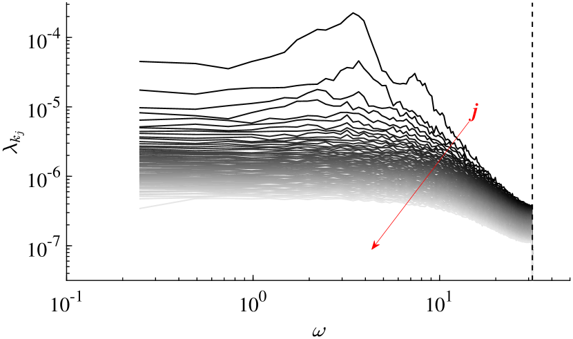
a

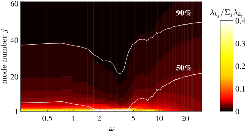
b

c

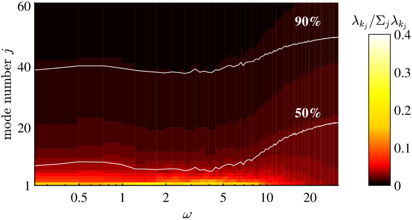
d

Figure 4: SPOD mode energy spectrum. The left column shows the spectral curves with the shading of the line color representing the increase in the mode number. The right column shows the percentage of energy that each mode accounts for as a function of frequency, with solid lines indicating that the cumulative energy represents $50\%$ and $90\%$ of the total energy at each frequency. (a,b) Symmetric component; (c,d) antisymmetric component.

SPOD solves the eigenvalue problems at each discrete frequency independently, and produces energy-ranked eigenvalues. Therefore, the energy distributions of different modes at each frequency can be best visualized in the form of a spectrum (Schmidt et al., 2018). The left column in figure 4 shows SPOD spectra for both symmetric and antisymmetric components. Meanwhile, the cumulative energy content and the percentage of energy accounted for by each mode as a function of frequency are shown in the right column. The symmetric component displays a higher overall energy level compared to the antisymmetric component, indicating its dominant role in the dynamics of the turbulent wake. The low-rank behavior, characterized by a large separation between the first and second modes, also appears to be more pronounced in the symmetric component. In particular, in the angular frequency ranges of $2<\omega<4$ of the symmetric component, the first modes contribute more than $50\%$ of the fluctuating energy according to figure 4(b). The frequency of the dominant symmetric coherent structure is $\omega=3.437$ as shown in figure 4(a). Additionally, the spectral energy concentration at $\omega\approx 6.9$, and a less pronounced peak around $\omega\approx 1.7$ can be identified respectively. These two angular frequencies could be associated with the first harmonic and subharmonic of the fundamental instability. This will be further investigated by checking the mode bi-spectrum, as the SPOD spectral curves cannot give direct insight into the frequency triads.

Figure 5: Spatial distribution of the most dominated SPOD mode ($\omega=3.437$) visualized based on iso-surface of the streamwise velocity component.

In figure 5, the spatial distribution of the leading SPOD mode is visualized based on the iso-surface of the streamwise velocity component. Overall, the three-dimensional mode is characterized by structures of different scales and shapes at different locations, which should be attributed to the complexity of the mean flow. In the near wake region, spanwise coherent vortex shedding can be observed from the recirculation region just behind the train tail. The coherent structures generated in span move downstream and gradually approach the ground due to effect of the moving ground (Wang et al., 2023). Meanwhile, we can also observe that the upper spanwise coherent structure rolls up at both lateral ends, and gradually stretches to be inclined in downstream direction due to its interaction with the longitudinal vortex pair. Once fully attached to the ground, the spanwise structures vanish and separate at the symmetry plane to evolve into far wake coherent structures at $x/W>1.5$. The far wake coherent structure displays a nearly constant streamwise wavelength, indicating that the far wake can be considered as nearly parallel in the streamwise direction.

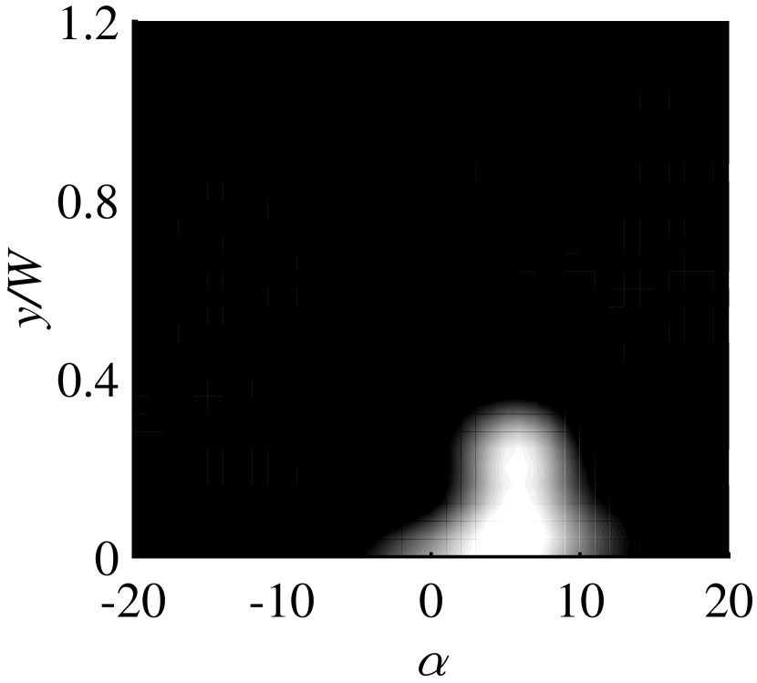
a

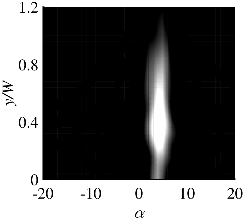
b

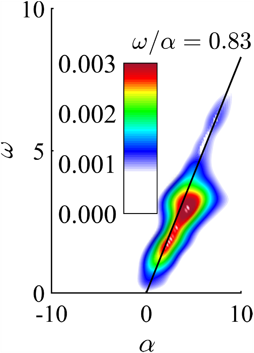
c

Figure 6: Streamwise wavenumber based on SPOD modes. (a) $0<x/H<1$ at $\omega=3.437$; (b) $1<x/H<6.67$ at $\omega=3.437$; (c) Angular frequency - streamwise wavenumber diagram.

To better quantify the frequency-wavenumber characteristics, a streamwise Fourier transform is applied to the streamwise velocity component of the SPOD modes, to convert the signal into the domain of streamwise wavenumber $\alpha$. Due to the dominant role of the symmetric perturbation in the wake, only symmetric modes are considered. First, the power spectral density (PSD) of the leading mode is averaged along the vertical direction, and plotted as a function of spanwise location and streamwise wavenumber in figure 6(a,b). Meanwhile, we isolate the mechanism in near wake and far wake regions by using two different window functions that constrain the signal to $0<x/W<1$ and $1<x/W<6.67$. The results are shown in figure 6(a) and figure 6(b), respectively. In the near-wake region, the maximum PSD is located in the symmetric plane, with $\alpha\approx 8$. We can also observe that the high PSD value occurs over a wide range of $\alpha$, which can be attributed to the growth of the wavelength of the spanwise vortex shedding mode. In the far wake region, the coherent structure has a nearly constant streamwise wavenumber, with the maximum PSD located away from the symmetry plane. This is consistent with what is shown in figure 5. Then for the first SPOD mode at all discrete frequency points, a window function including both near-wake and far-wake is used to compute the PSD distribution, followed by the averaging over all cross-flow locations, to construct the frequency-wavenumber diagram shown in figure 6(c). In general, a constant phase velocity of 0.83 can be observed across the angular frequency range. This value is typical of the Kelvin-Helmholtz instability wave and is related to the shear layer of the far wake counter-rotating vortex pair. Since the frequency-wavenumber diagram includes both near-wake and far-wake instability waves, the phase velocity tends to decrease at frequencies with a pronounced low rank due to the near-wake mode.

3.4 Triadic interactions

A frequency triad is described by the interaction of two structures at frequencies $\omega_{k}$ and $\omega_{l}$, resulting in a third structure at frequency $\omega_{k+l}$, obeying the condition $\omega_{k}\pm\omega_{l}\pm\omega_{k+l}=0$. As introduced previously, the SPOD energy spectrum shows at which frequency the flow is dominated by coherent structures, but does not contain information on frequency triads. In our case, the harmonic triads and the broadband low-rank behavior are of great importance for a more detailed interpretation of the wake dynamics. Here, bispectral mode decomposition (Schmidt, 2020) is used to estimate the mode bispectrum

For a given one-dimensional signal $q(t)$, the bispectrum can be expressed as

$$\mathbf{S}_{qqq}\left(k,l\right) =\int_{-\infty}^{\infty}\int_{-\infty}^{\infty}E\left[q(t)q(t-\tau_{k})q(t-\tau_{l})\right]{\rm{exp}}({-\rm{i}}(\omega_{k}\tau_{k}+\omega_{l}\tau_{l})){\rm{d}}\tau_{k}{\rm{d}}\tau_{l}$$ (13)

$$=\lim\limits_{T\to\infty}\frac{1}{T}E\left[\hat{q}(\omega_{k})^{\ast}\hat{q}(\omega_{l})^{\ast}\hat{q}(\omega_{k}+\omega_{l})\right]$$

where the superscript $\left(.\right)^{\ast}$ is the scalar complex conjugate, $E\left[.\right]$ is the expectation value, $\tau$ is the time lag, and $\hat{q}(\omega_{k})$ and $\hat{q}(\omega_{l})$ are the $k$-th and $l$-th components of $\hat{q}$.

The BMD constitutes an analogy to the classical bispectrum for multidimensional signals (Schmidt & Oberleithner, 2023). The principle of BMD is to construct

$$b\left(\omega_{k},\omega_{l}\right)\equiv{E}\left[\int_{\Omega}\hat{\mathbf{q}}_{k}^{\ast}\circ\hat{\mathbf{q}}_{l}^{\ast}\circ\hat{\mathbf{q}}_{k+l}\rm{d}\mathbf{x}\right]=E\left[\hat{\mathbf{q}}_{k\circ{l}}^{H}\mathbf{W}\hat{\mathbf{q}}_{k+l}\right]$$ (14)

where $\circ$ denotes the spatial entry-wise product, and $\hat{\mathbf{q}}_{k\circ{l}}$ the shorthand for $\hat{\mathbf{q}}_{k}\circ\hat{\mathbf{q}}_{l}$. To give the approximation of the expectation value, again the DFT realizations of $\hat{\mathbf{q}}_{k\circ{l}}$ and $\hat{\mathbf{q}}_{k+{l}}$ are rearranged into

$$\mathbf{\hat{Q}}_{k\circ{l}} \equiv\begin{bmatrix}\mathbf{\hat{q}}^{(1)}_{k\circ{l}}&\ \mathbf{\hat{q}}^{(2)}_{k\circ{l}}&...&\mathbf{\hat{q}}^{(n_{\rm{blk}})}_{k\circ{l}}\end{bmatrix}$$ (15a)

$$\mathbf{\hat{Q}}_{k+{l}} \equiv\begin{bmatrix}\mathbf{\hat{q}}^{(1)}_{k+{l}}&\ \mathbf{\hat{q}}^{(2)}_{k+{l}}&...&\mathbf{\hat{q}}^{(n_{\rm{blk}})}_{k+{l}}\end{bmatrix}$$ (15b)

Then the bispectral modes $\mathbf{\phi}_{k+{l}}$, which are linear combinations of Fourier modes, and cross-frequency fields $\mathbf{\phi}_{k\circ{l}}$, which are maps of phase alignment between two frequency components, are introduced. These two fields share a common set of expansion coefficients, $\mathbf{a}_{i}$, which expand the vectors into the spaces spanned by the ensembles of realizations of $\mathbf{\hat{q}}_{k+{l}}$ and $\mathbf{\hat{q}}_{k\circ{l}}$. A compact form can be given as

$$\mathbf{\phi}^{(i)}_{k\circ{l}} =\mathbf{\hat{Q}}_{k\circ{l}}\mathbf{a}_{i}$$ (16a)

$$\mathbf{\phi}^{(i)}_{k+l} =\mathbf{\hat{Q}}_{k+l}\mathbf{a}_{i}$$ (16b)

By now, the goal of BMD is to seek the set of expansion coefficients $\mathbf{a}_{1}$ that maximizes the absolute value of $b\left(\omega_{k},\omega_{l}\right)$. To find the optimal $\mathbf{a}_{1}$, the weighted bispectral density matrix is introduced.

$$\mathbf{B}=\frac{1}{n_{\rm{blk}}}\mathbf{\hat{Q}}_{k\circ{l}}^{H}\mathbf{W}\mathbf{\hat{Q}}_{k+l}$$ (17)

It can be the found that the maximize problem is equivalent to finding the vector $\mathbf{a}_{1}$ associated with the numerical radius of $\mathbf{B}$

$$r(\mathbf{B})={\rm{max}}\left|\frac{\mathbf{a}_{1}^{H}\mathbf{B}\mathbf{a}_{1}}{\mathbf{a}_{1}^{H}\mathbf{a}_{1}}\right|$$ (18)

Then this value is referred as the complex mode bispectrum. For a detailed mathematical derivation and algorithmic implementation, the reader is referred to Schmidt (2020).

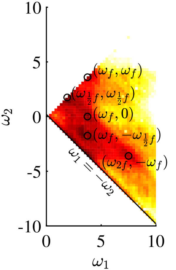
a

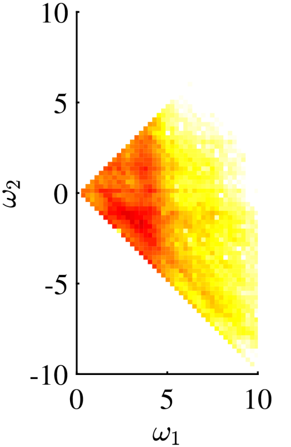
b

c

Figure 7: Mode bispectrum in both the sum and difference regions. (a) Self interaction of symmetric component; (b) Interaction of symmetric and antisymmetric components with $\omega_{1}$ the symmetric component and $\omega_{2}$ the antisymmetric component; (c) Interaction of symmetric and antisymmetric components with $\omega_{1}$ the antisymmetric component and $\omega_{2}$ the symmetric component.

Here, the mode bispectrum is computed using the same spectral estimation parameters as in the SPOD of $\S$3.2. Due to the high-energy contribution of the symmetric component, both its self-interaction and the interaction with the antisymmetric component are of interest to study. Note that the third frequency component resulting from the mutual interaction of symmetric and antisymmetric components is always antisymmetric.

In figure 7, the mode bispectrum are shown. Here, the self-interaction of the symmetric component shown in figure 7(a) is identified with several distinct peaks, while the interaction between symmetric and antisymmetric components presented in figure 7(b,c) contains less information and therefore is not interpreted. We refer to $\omega_{f}$ as the fundamental frequency detected in SPOD. Conceptually, the triplet $(\omega_{f},0,\omega_{f})$ on the mode bispectrum can be regarded as the coherent perturbation driven by the mean flow. However, in BMD, only quadratic terms are considered, so the value on the $\omega_{1}$-axis should not be interpreted. Then a local maximum of the distribution can be found that corresponds to the sum interaction of the fundamental instability with itself, generating the first harmonic at twice the fundamental frequency via the triad $(\omega_{f},\omega_{f},2\omega_{f})$. At the same time, the doublets $(2\omega_{f},-\omega_{f})$ and $(\frac{1}{2}\omega_{f},\frac{1}{2}\omega_{f})$, which include the first harmonic and subharmonic, respectively, feed back into $\omega_{f}$. Then the triad $(\omega_{f},-\frac{1}{2}\omega_{f},\frac{1}{2}\omega_{f})$ can also be found that contributes to the subharmonic frequency. The mean field distortion, indicated by the peak values along line $\omega_{1}=-\omega_{2}$ can be identified over a wide frequency range.

Based on the presented results, the important dynamics that characterize the frequency-domain energy distribution of the flow can be explained as follows: As the flow oscillates at $\omega_{f}$, the dominant coherent structure meanwhile drives its first harmonic and subharmonic through the energy cascade process. These coherent structures interact with each other through multiple triads and feed back into the related frequencies. At the same time, they continuously modify the mean field and lead to distortion of the base flow. As the dominant coherent structure is driven by the mean flow, its oscillating frequency constantly deviates from $\omega_{f}$. With the continuous evolution of the described process, the flow finally appears to be low-rank in the wide frequency range as shown in figure 4.

4 Physics-based coherent structure modelling

Linear global stability analysis is conducted to identify the mechanisms that drive the dominant coherent structure identified in the SPOD. In this work, instead of directly solving the three-dimensional stability equation, we conduct a two-dimensional local analysis to obtain more local information while reducing computational resource. In this manner, the flow is assumed to be weakly nonparallel in the streamwise direction. Then the full three-dimensional matrix eigenvalue problem is replaced by several local independent matrix problems, each based on the two-dimensional cross-flow planes at different streamwise locations. To determine the global mode, the concept of local convective / absolute instability is applied within the WKBJ approximation (Huerre & Monkewitz, 1990). To be clear, the approach used in the research does not conceptually correspond to the bi-global analysis (Theofilis, 2011), but is similar to the approach used in Huerre & Monkewitz (1990); Monkewitz et al. (1993); Juniper et al. (2014), in which the bi-global stability is approximated using one-dimensional local analysis.

4.1 Linearized operator and treatment of the nonparallel flow

Coherent structures can be described by the triple decomposition (Reynolds & Hussain, 1972), which leads to a further decomposition of the fluctuating component into coherent and stochastic parts as

$$\mathbf{q}^{\prime}(\mathbf{x},t)=\mathbf{\widetilde{q}}(\mathbf{x},t)+\mathbf{q}^{\prime\prime}(\mathbf{x},t)$$ (19)

where $\mathbf{\widetilde{q}}(\mathbf{x},t)$ is the coherent fluctuation part and $\mathbf{q}^{\prime\prime}(\mathbf{x},t)$ is the stochastic fluctuation part. This decomposition is substituted into both the momentum and continuity equations, and both are time-averaged and phase-averaged. Then by subtracting the time-averaged set of equations from the phase-averaged set of equations, the equations governing the evolution of coherent structures can be written (Reynolds & Hussain, 1972)

$$\frac{\partial{\mathbf{\widetilde{u}}}}{\partial{t}}+(\mathbf{\widetilde{u}}\cdot\nabla)\mathbf{\bar{u}}+(\mathbf{\bar{u}}\cdot\nabla)\mathbf{\widetilde{u}}=-\nabla{\widetilde{p}}+\nabla\cdot\left(\frac{1}{\mathit{Re}}(\nabla+\nabla^{\rm{T}})\mathbf{\widetilde{u}}\right)-\nabla\cdot\left(\tau_{R}+\tau_{N}\right)$$ (20)

$$\nabla\cdot\mathbf{\widetilde{u}}=0$$ (21)

Here $\tau_{N}$ describes the quadratic interactions of the coherent perturbation. Considering that the energy contribution from this process is higher-order, this term is neglected in the following. The term $\tau_{R}$ is the fluctuation of the stochastic Reynolds stresses related to the stochastic-coherent interaction, which contributes at leading order, according to the energy considerations of Reynolds & Hussain (1972), and is therefore retained in the equation. However, this term is not known a priori and needs to be properly modeled to close the governing equation. In this paper, we use Boussinesq’s eddy viscosity model as the closure. The Reynolds stresses are then expressed as

$$\tau_{R}=-\nu_{t}\left(\nabla+\nabla^{\rm{T}}\right)\mathbf{\widetilde{u}}.$$ (22)

Here $\nu_{t}$ is the normalized eddy viscosity, which can be calculated using quantities of the LES mean flow. Since this approach yields an eddy viscosity for each independent Reynolds Stress component, a reasonable compromise would be to take the least mean square of the six values.

$$\nu_{t}=\frac{\left<-\overline{\mathbf{u}^{\prime}\mathbf{u}^{\prime}}+2/3k\mathbf{I},\bar{\mathbf{S}}\right>_{\rm{F}}}{2\left<\bar{\mathbf{S}},\bar{\mathbf{S}}\right>_{\rm{F}}}$$ (23)

with $\left<\cdot,\cdot\right>_{\rm{F}}$ denoting the Frobenius inner product, $k$ the kinetic energy, $\mathbf{I}$ the identity matrix and $\bar{\mathbf{S}}$ the mean shear strain rate tensor. This approach has been widely used in the linear stability analysis of turbulent flows, as presented in Tammisola & Juniper (2016); Rukes et al. (2016); Kaiser et al. (2018); Müller et al. (2020); Kuhn et al. (2021).

The linearized momentum and continuity equations for the coherent perturbation can be obtained as

$$\frac{\partial{\mathbf{\widetilde{u}}}}{\partial{t}}+(\mathbf{\widetilde{u}}\cdot\nabla)\mathbf{\bar{u}}+(\mathbf{\bar{u}}\cdot\nabla)\mathbf{\widetilde{u}}=-\nabla{\widetilde{p}}+\nabla\cdot\left(\left(\frac{1}{\mathit{Re}}+\nu_{t}\right)(\nabla+\nabla^{\rm{T}})\mathbf{\widetilde{u}}\right)$$ (24)

$$\nabla\cdot\mathbf{\widetilde{u}}=0.$$ (25)

These equations can be then rewritten as

$$\mathbf{\mathcal{L}}\mathbf{\widetilde{q}}=0$$ (26)

where $\mathbf{\mathcal{L}}$ is the operator of the linearized equations superimposing the spatial discretization and base state (Paredes et al., 2013).

By assuming that the mean field has much smaller derivatives in the streamwise direction than in the transverse and vertical directions, the system can be Fourier-transformed in the streamwise direction, following the streamwise weakly nonparallel flow assumption. The coherent perturbation can be then written as

$$\widetilde{q}(x,y,z,t)=\hat{q}(y,z){\rm{exp}}\left[{\rm{i}}\left(\alpha{x}-\omega{t}\right)\right]+\rm{c.c}.$$ (27)

where $\mathbf{\hat{q}}$ is the complex eigenfunction, $\alpha=\alpha_{\rm{r}}+\rm{i}\alpha_{\rm{i}}$ is the complex streamwise wavenumber, $\omega=\omega_{\rm{r}}+\rm{i}\omega_{\rm{i}}$ is the complex angular frequency, and c.c. is the complex conjugate. Substituting equation 27 into equation 26 enables stability analysis of the mean field in the cross-flow plane at different streamwise locations. The global stability characteristics can then be recovered based on the concept of absolute/convective instability and the global mode wavemaker (Huerre & Monkewitz, 1990).

However, using the local approach to predict the global mode has been reported to be less accurate than the direct global approach, when the base flow is strongly nonparallel (Juniper et al., 2011; Juniper & Pier, 2015). In the current case, where a fully developed three-dimensional base flow is considered, the parallel flow assumption is likely to introduce uncertainty into the results. Therefore, in this work, we also make further treatment to approximate the non-parallelism of the three-dimensional base flow.

The parallel flow assumption is checked by visualizing the streamwise component of the leading SPOD mode on a horizontal plane as shown in figure 8. Here the coherent perturbations can be observed with clear wavepacket structures; however, they do not travel strictly in the streamwise direction but follow oblique paths in both the near and far wake. This is caused by the downwash flow from the slanted tail surface which gradually separates the wake structures as it propagates downstream, as can be seen in the mean flow structures shown in figure 2.

We intend to account for the obliqueness of the coherent structure in the linear modeling. To do this, an expression related to the state vector can be written

$$\hat{q}(x_{0},y_{0},z_{0})=\hat{q}(x_{0}+\Delta{x},y_{0}+\rm{tan}\theta\Delta{x},z_{0}+{\rm{tan}}\gamma\Delta{x})$$ (28)

where $\rm{tan}\theta$ and $\rm{tan}\gamma$ respectively represent the convection direction relative to symmetric plane and horizontal plane. By applying a first-order Taylor expansion to the right-hand side of equation 28, the left-hand side can be canceled and the expression can be arranged into

$$\frac{\partial{\mathbf{\hat{q}}}}{\partial{x}}+{\rm{tan}}\mathbf{\theta}\frac{\partial{\mathbf{\hat{q}}}}{\partial{y}}+{\rm{tan}}\mathbf{\gamma}\frac{\partial{\mathbf{\hat{q}}}}{\partial{z}}=0$$ (29)

This, an artificial $x$-derivative applied to the state vector $\mathbf{\hat{q}}$ is used to account for the oblique traveling direction.

To determine $\rm{tan}\theta$ and $\rm{tan}\gamma$, we replace $\mathbf{\hat{q}}$ with mean field quantities $\mathbf{\bar{q}}$ in equation 29, by assuming that the perturbation waves follow the mean flow convection. Note that, for each node in the computational domain, the four flow variables are used to construct the linear equation system for $\rm{tan}\theta$ and $\rm{tan}\gamma$ and the final results are obtained using the least-squares solution of the overdetermined linear equation system.

Finally, the convection direction calculated from the mean field is validated by comparison with the oblique path of the SPOD mode. In figure 8, streamlines based on the calculated local angle $\theta$ are visualized, by decomposing $\rm{tan}\theta$ at each computational node into streamwise ($\rm{cos}\theta$) and transverse ($\rm{sin}\theta$) components using trigonometric functions. It can be observed that the vector field agrees well with the traveling direction of the SPOD wavepackets. Therefore, the artificial $x$-derivative is assumed to be reasonable to account for the obliqueness of the coherent structure in the linear modelling.

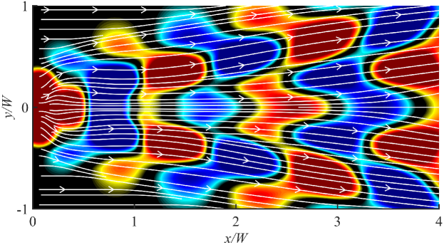
Figure 8: Two-dimensional slice of the streamwise component of three-dimensional SPOD mode showing the oblique downstream traveling wavepackets. The streamlines are drawn based on the vector field ($\rm{cos}\theta$, $\rm{sin}\theta$) at each computational node.

4.2 Spatio-temporal stability approach

For the linear stability analysis, the linear operator $\mathbf{\mathcal{L}}$ is rearranged to construct the generalized eigenvalue problem. In this work, both the temporal and spatial stability formulation is needed. Therefore, either the temporal stability form

$$\mathbf{\mathcal{A}}(x,\alpha)\mathbf{\hat{q}}=\omega\mathbf{\mathcal{B}}(x)\mathbf{\hat{q}}$$ (30)

or the spatial stability form

$$\mathbf{\mathcal{A}}(x,\omega)\mathbf{\hat{q}}=\alpha\mathbf{\mathcal{B}}(x)\mathbf{\hat{q}}$$ (31)

are constructed.

In the temporal stability form (equation 30), the streamwise wavenumber $\alpha$ is fixed to a real value, and the eigenvalue problem is solved for a complex $\omega$, the real part of which is the angular frequency and the imaginary part is the temporal growth/decay rate. On the contrary, in the spatial stability form (equation 31), a real angular frequency $\omega$ is imposed to search for the complex $\alpha$, where the real part corresponds to the streamwise wavenumber, while the imaginary part is the spatial amplification/damping rate. Note that, in the spatial stability equation, quadratic terms appear with respect to $\alpha$. This problem is solved using the companion matrix method (Bridges & Morris, 1984), which increases the size of the eigenvalue problem compared to the temporal analysis. The complete expression of the operators $\mathbf{\mathcal{A}}$ and $\mathbf{\mathcal{B}}$ for both temporal and spatial analysis can be found in Appendix A.

To determine the global stability of the mean flow from a local analysis, a so-called spatio-temporal analysis using equation 30 must be performed to distinguish between convective and absolute instability (Huerre & Monkewitz, 1990). In this case, both $\alpha$ and $\omega$ are complex-valued. Conceptually, the flow is said to be stable if all perturbations decay in time throughout the entire domain after a localized impulse. Convectively unstable flow gives rise to perturbations that grow in time but convect away from the impulse location, so that the perturbations eventually decay to zero at each spatial location in the long time limit. For an absolutely unstable flow, the perturbations grow both upstream and downstream of the impulse location, contaminating the whole spatial domain in the long time limit.

Based on the previous definitions, the convective/absolute nature of a local velocity profile can be determined from the time-asymptotic behavior of the perturbations that remain at the impulse location, that is, for perturbations with zero group velocity: $\partial\omega/\partial\alpha=0$, which is the definition of a saddle point in the complex $\alpha-$plane. Therefore, valid saddle points on the complex $\alpha$-plane that satisfy the Briggs-Bers pinch-point criterion (Briggs, 1964) must be identified. Therefore, the flow is locally absolutely unstable if the absolute growth rate, given by the imaginary part of $\omega$ at the most unstable valid saddle point, is positive. If the absolute growth rate is negative, the flow is convectively unstable or stable (Huerre & Monkewitz, 1990; Rees & Juniper, 2010; Juniper et al., 2014; Rukes et al., 2016; Kaiser et al., 2018; Demange et al., 2020).

In a spatially developing flow, a region of absolute instability is a necessary (but not sufficient) condition for global instability (Monkewitz et al., 1993; Chomaz, 2005). To further link the local absolute instability to global instability, the absolute growth rate needs to be tracked along the streamwise direction to determine the wavemaker, the location where the global mode is selected. This method has been extensively used for one-dimensional local stability analysis in comparison with bi-global stability analysis (Giannetti & Luchini, 2007; Juniper et al., 2011; Juniper & Pier, 2015; Kaiser et al., 2018).

4.3 Solving the eigenvalue problem

To solve the eigenvalue problem numerically, cross-flow planes with the dimensions of $0{\leq}y/H{\leq}1.3$ and $0{\leq}z/H{\leq}1.3$ are discretized using Chebyshev spectral collocation methods. This approach has been successively applied to linear stability analysis by Khorrami (1991); Parras & Fernandez-Feria (2007); Oberleithner et al. (2011); Demange et al. (2020). Detailed descriptions or practical guides to spectral collocation methods can be found in Khorrami et al. (1989); Trefethen (2000).

To reduce the numerical cost, we further exploit the symmetry of the mean field with respect to the vertical $x$-$z$ plane. This allows us to use only half of the wake plane instead of the full plane, to compute only transversely symmetric or antisymmetric eigenmodes when appropriate boundary conditions are applied (Zampogna & Boujo, 2023). As shown in $\S$3, the symmetric perturbations are dominant and potentially related to a global instability, so only symmetric eigenmodes are considered. The corresponding boundary conditions are given as

$$\frac{\partial{\mathbf{\hat{u}}}}{\partial{y}}=\frac{\partial{\mathbf{\hat{w}}}}{\partial{y}}=\frac{\partial{\mathbf{\hat{p}}}}{\partial{y}}=0,\mathbf{\hat{v}}=0\ {\rm{on}}\ y/W=0$$ (32a)

$$\frac{\partial{\mathbf{\hat{u}}}}{\partial{y}}=\frac{\partial{\mathbf{\hat{v}}}}{\partial{y}}=\frac{\partial{\mathbf{\hat{w}}}}{\partial{y}}=\frac{\partial{\mathbf{\hat{p}}}}{\partial{y}}=0\ {\rm{on}}\ y/W=1.3$$ (32b)

$$\mathbf{\hat{u}}=\mathbf{\hat{v}}=\mathbf{\hat{w}}=0,\frac{\partial{\mathbf{\hat{p}}}}{\partial{z}}=0\ {\rm{on}}\ z/W=0$$ (32c)

$$\mathbf{\hat{u}}=\mathbf{\hat{v}}=\mathbf{\hat{w}}=\mathbf{\hat{p}}=0\ {\rm{on}}\ z/W=1.3$$ (32d)

Here, equation 32$a$ determines eigenmodes to be transversely symmetric. At the wall, homogeneous Dirichlet boundary conditions are imposed for the velocity components. For pressure, by substituting the homogeneous Dirichlet conditions for velocity into equation 24, a compatibility condition can be obtained (Theofilis et al., 2004). Here, assuming $\partial^{2}{\mathbf{\hat{w}}}/\partial{z}^{2}=0$ gives a homogeneous Neumann condition for the pressure. For far-field boundaries, the upper boundary is set to a homogeneous Dirichlet condition, while the side boundary is set to a homogeneous Neumann condition which is necessary to predict far wake eigenmodes.

The Krylov-Schur algorithm (Stewart, 2002), which serves as an improvement on traditional Krylov subspace methods such as the Arnoldi and Lanczos algorithms, is used to obtain a subset of solutions to the eigenvalue problem. This requires an initial guess of the physical eigenvalue, which can be derived from the dispersion relation shown in $\S$3.3. To discard spurious eigenmodes caused by the discretization, two criteria are applied: First, all eigenmodes that do not diminish when approaching the upper boundary are discarded. Second, since spurious eigenvalues are very sensitive to discretization, a convergence study of eigenvalues computed using different grid resolutions is used as a criterion for filtering spurious eigenvalues.

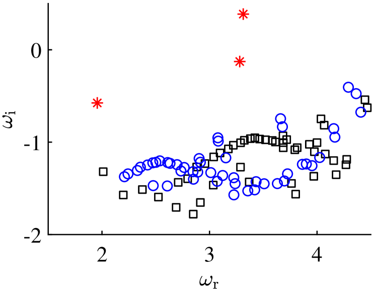
a

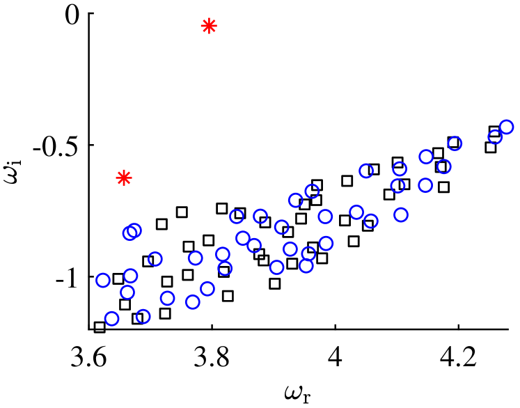
b

Figure 9: The spectrum of eigenvalues obtained with discretization points of 8,100 ( $\square$ ) and 10,000 ($\color[rgb]{0,0,1}\circ$), the physical eigenvalues are marked with $\color[rgb]{1,0,0}\ast$. (a) results based on cross-flow plane at $X/W=0.1$ and imposing $\alpha=10$. (a) results based on cross-flow plane at $X/W=3.5$ and imposing $\alpha=5$.

The results of the convergence study based on temporal stability analysis are shown in figure 9. Two representative cross-flow planes, located in the near-wake and far-wake, respectively, are considered. Real streamwise wavenumbers of 10 and 5 are, respectively, imposed in the two eigenvalue problems, which are then discretized using two different grid resolutions and solved for the subset of the eigenvalue spectrum. Note that the real streamwise wavenumbers are chosen according to the wavelength distribution of the dominant SPOD mode shown in figure 6, so that the SPOD peak frequency can be set as the initial value of the Krylov-Schur iteration procedures. As shown in figure 9, both spectra feature continuous branches and a set of discrete modes. In general, continuous branches are made up of spurious eigenmodes caused by discretization and physical eigenmodes that are highly stable.

It can be observed that the locations of these eigenmodes in continuous branches vary significantly when the resolution of the grid is changed. On the contrary, the locations of the discrete modes remain almost stationary with different discretization settings; hence, the discrete modes are considered as physical eigenmodes that can potentially contribute to global instability. In particular, the near-wake cross-flow plane features one unstable mode and two stable modes, while the far-wake plane features two stable modes. Note that these physical eigenvalues do not necessarily correspond between the near-wake and far-wake cross-flow planes. When tracking along the streamwise direction, the physical eigenvalues may become highly stable and fall into the spurious region, and new physical eigenvalues may emerge due to the complexity of the base flow.

4.4 Absolute/convective stability analysis

4.4.1 Streamwise evolution of temporal growth rate

Before considering the absolute / convective nature of the instability, it is necessary to know which part of the flow is temporally unstable. To this end, a Newton-Raphson iterative method Ypma (1995) is used to vary the real wavenumber $\alpha$ and to determine the maximum temporal growth rate of each previously identified physical mode. This procedure is repeated at each streamwise position to track the maximum temporal growth rates of all physical eigenmode. As mentioned above, due to the complexity of the base flow, one physical eigenmode may occur only in a certain range of streamwise location. Therefore, several cross-flow planes are used to compute the physical eigenvalues, and then the tracking process is repeated to account for the maximum temporal growth rates of all physical eigenmodes in the entire wake.

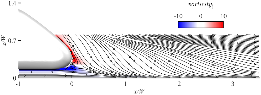
a

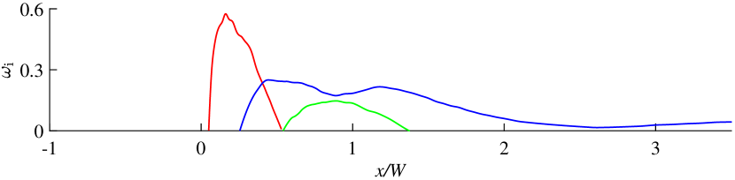
b

Figure 10: Maximum temporal growth rate as functions of streamwise location. (a) Mean flow distribution in the central plane. (b) maximum temporal growth rate of near wake ( ), middle wake ( ) and far wake ( ) eigenmodes with real $\alpha$ imposed.

In figure 10, the maximum temporal growth rates of these physical eigenmodes are displayed as a function of streamwise location. Only the unstable regime ($\omega_{\rm{i}}>0$) is shown here. Three different unstable eigenvalue branches are identified in the entire wake, each dominating in different streamwise regions. Accordingly, the flow becomes temporally unstable very close to the tail of the train and remains unstable in the wake. Based on the spatial locations where these branches become unstable, we conceptually divide the wake into the near, middle, and far wake regimes and name these branches accordingly. It can be found in figure 10(b) that the near wake eigenmode is temporally more unstable than all the downstream eigenmodes. According to the mean flow distribution shown in figure 10(a), this eigenmode branch is attributed to the transverse recirculation zone located right behind the tail of the train. The far wake eigenmode can be observed across a wide streamwise distance and is located closely to the extension of the streamwise vortex pair. This branch has the largest temporal growth rate at $x/W\sim 0.4$, and gradually stabilizes as it extends into the far wake; however, it remains still unstable. The middle wake mode becomes unstable at $0.5<x/W<1.4$. At this location, with respect to the mean field, the flow from the slanted tail surface can be observed attached to the ground according to the figure 10(a).

4.4.2 Spatio-temporal stability analysis in the near wake

Spatio-temporal analysis is performed to compute the contour of $\omega$ in the complex $\alpha$-plane, so as to find valid saddle points following the Briggs-Bers criterion. Since the branch in the near-wake region is temporally more unstable than the other branches (figure 10), we start with the near-wake branch.

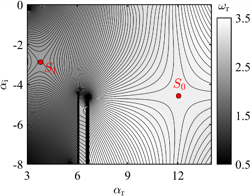
a

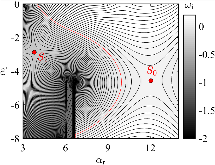
b

Figure 11: Contour of the complex angular frequency in the complex $\alpha$-plane at $x/W=0.08$. Saddle points on the complex $\alpha$-plane are marked by a red circle. (a) The real component; (b) The imaginary component, and the $\omega_{\rm{i}}=0$ isocontour is highlighted in red.

Figure 11 shows the contour of the complex frequency in the complex $\alpha$-plane, at the streamwise location of $x/W=0.08$. At this location, the near-wake eigenmode reaches its maximum temporal growth rate. In this figure two saddle points are found, $S_{0}$ and $S_{1}$. However, valid saddles must be pinched between an $\alpha^{+}$ and an $\alpha^{-}$ branch (Huerre & Monkewitz, 1990). A simple rule based on the Briggs-Bers pinch point criterion (Briggs, 1964) can be applied by checking the isocontours of the spatio-temporal growth rate (figure 11(b)): Starting from the saddle point, the contours of the growing $\omega_{\rm{i}}$ must reach, respectively, the $\alpha_{\rm{i}}>0$ and $\alpha_{\rm{i}}<0$ half-planes. Here, the validity of both $S_{0}$ and $S_{1}$ can be confirmed, with $S_{0}$ representing the shorter traveling wave at higher frequency, while $S_{1}$ represents the longer traveling wave at lower frequency. In the long time limit, the nature of the instability is determined by $S_{0}$, which has a significantly higher absolute growth rate than $S_{1}$. Then the absolute frequency at this location can be determined as $\omega_{0}=3.2904+0.0685{\rm{i}}$, which shows that the flow is absolutely unstable at this position.

Furthermore, to ensure that all regions with absolute instability have been taken into account, the absolute growth rate has been determined for all unstable branches at several streamwise locations. The near wake branch was the only one to reveal absolute instability.

4.5 Determining the global mode wavemaker in the near wake

To determine the global mode, the saddle points are tracked in the stream direction to find the global wavemaker. This is done in the local analysis framework based on the frequency selection criterion. Several criteria have been evaluated in Pier (2002), showing that the criterion for a linear global mode introduced by Chomaz et al. (1991) agrees best with the nonlinear direct numerical simulations. This criterion is obtained from an analytical continuation of the absolute frequency curve into the complex $x$-plane. The wavemaker region is then represented by the saddle point on the complex $x$-plane (Huerre & Monkewitz, 1990) defined as

$$\frac{\partial\omega_{0}}{\partial{x}}(x_{\rm{s}})=0$$ (33)

The global complex angular angular frequency is then given by the value of the absolute frequency at this saddle point

$$\omega_{\rm{g}}=\omega_{0}(x_{\rm{s}}).$$ (34)

For this purpose, the saddle point $S_{0}$ found in figure 10 is tracked along the streamwise direction. The three-point Taylor series expansion algorithm (Rees, 2010) is used to approach $\partial\omega/\partial\alpha=0$ during the tracking process. Then the absolute frequency as a function of streamwise location is analytically continued in the complex $x$-plane using the Padé polynomial, which has been shown to be well behaved in the complex plane (Cooper & Crighton, 2000). The Padé polynomial takes the form of

$$f(x)=\frac{P(x)}{Q(x)}=\frac{a_{0}+a_{1}x+...+a_{n}x^{n}}{1+b_{1}x+...+b_{m}x^{m}}$$ (35)

To determine the order of the polynomials used in the current work, the procedure described in Juniper et al. (2011) is followed. Polynomials of order 10 have been proven to be sufficient to give a converged approximation of the saddle point.

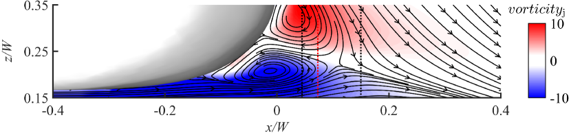
a

b

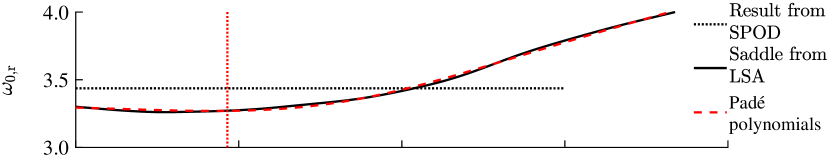
c

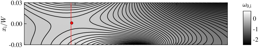
d

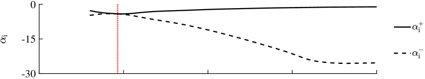
e

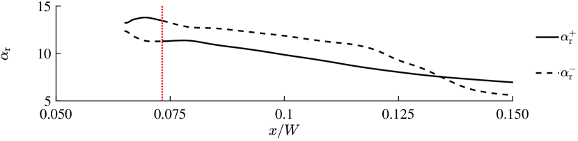
f

Figure 12: (a) Streamlines and through-plane vorticity of the mean fiwld in the near wake region. (b) Streamwise evolution of the absolute growth rate. (c) Streamwise evolution of the absolute angular frequency. (d) Contours of $\omega_{\rm{0,i}}$ extruded in the complex $x$-plane, formed by the fitted Padé polynomial. The saddle point on the complex $x$-plane is marked by red circle. (e) The imaginary component of local complex streamwise wavenumber of $\alpha^{+}$ and $\alpha^{-}$ branches calculated at the global frequency $\omega_{g}$. (f) The same as (e) with the real component shown. The switching locations between $\alpha^{+}$ and $\alpha^{-}$ branches are marked by a red vertical line in each sub-figure.

Figure 12 shows the main results of the spatio-temporal stability analysis. For reference, the mean field in the central plane is shown in figure 12(a). The following rows include the results of the procedures described above to determine the global instability using local analysis. In figure 12(b,c), the imaginary and real parts of the absolute complex angular frequency are shown as a function of streamwise location, respectively. A small region of absolute instability is detected, which is located in the recirculation region. The 10th order Padé polynomials show acceptable agreement with the absolute frequency curve of the linear stability analysis. The extrapolated complex $x$-plane is then visualized in figure 12(d). The saddle point appears to be very close to the real axis, with $x_{\rm{s}}=0.0733+0.0010{\rm{i}}$, indicating a wavemaker located within the region of absolute instability. The complex global angular frequency associated with this saddle point is $\omega_{\rm{g}}=3.2702+0.0797{\rm{i}}$.

The theoretically predicted global mode frequency can be compared to the frequency of the most energetic SPOD mode. With an empirical value of $\omega_{\rm{SPOD}}=3.437$, as shown in figure 4, we find that the theoretical prediction deviates by an error of less than $5\%$. This is in very good agreement, given the uncertainties introduced by the nonparallelism and eddy viscosity modeling. Moreover, we expect the global mode to be marginally unstable, representing a limit-cycle oscillation when stability analysis is performed on a temporally averaged mean flow (Noack et al., 2003; Barkley, 2006; Oberleithner et al., 2011; Rukes et al., 2016; Tammisola & Juniper, 2016; Kaiser et al., 2018). However, as reported in Giannetti & Luchini (2007); Juniper et al. (2011); Juniper & Pier (2015), it is a common feature of local analysis to overpredict the growth rate of the linear global mode. In our case, with a growth rate value of 0.0797, the relative error with respect to the real frequency (3.2702) is less than $3\%$, therefore, it is reasonable to say that the mode is marginally unstable. Overall, considering the fact that the flow is not truly parallel and the intrinsic assumption of linearized mean field analysis, it can be concluded that the theoretical mode identifies the dominant SPOD mode as a global mode at limit cycle with remarkable accuracy.

The global mode is formed by the switching between the $\alpha^{+}$ and $\alpha^{-}$ branches at the global frequency. Therefore, to further truly localize the global mode wavemaker, a spatial stability analysis (equation 31) imposing $\omega=\omega_{\rm{g}}$ is conducted to compute the $\alpha^{+}$ and $\alpha^{-}$ branches (Juniper & Pier, 2015). Since the saddle point $x_{\rm{s}}$ on the complex $x$-plane is very close to the real axis, the location of maximum structural sensitivity should also be close to $x_{\rm{s,r}}$. Therefore, in practice, it can be quite straightforward to find the branch pairs by computing the eigenvalue problem at $x/W=x_{\rm{s,r}}$, and following $\alpha_{\rm{i}}^{+}-\alpha_{\rm{i}}^{-}\approx 0$ in the streamwise direction.

In figure 12(e,f), the imaginary and real components of the $\alpha^{+}$ and $\alpha^{-}$ branches are presented, respectively. The switch between the two branches can be identified to take place at $x/W=0.0731$. The location of the global mode wavemaker is marked by a red vertical line in all sub-figures of figure 12. This location is also within the recirculation region and is nearly identical to the location of the saddle point $x_{\rm{s}}$. The direct global mode then follows the $\alpha^{-}$ branch upstream of the wavemaker, and the $\alpha^{+}$ branch downstream. In contrary, the adjoint global mode follows the $\alpha^{+}$ branch upstream of the wavemaker, and $\alpha^{-}$ branch downstream (Juniper & Pier, 2015). This result also indicates a spatially growing global mode within the recirculation region, with the growth rate gradually decaying to zero as it approaches the downstream boundary of this region.

In summary, we identify a global mode with a frequency very close to the dominant SPOD mode and a growth rate close to zero. This suggests that the dominant SPOD mode is a manifestation of a global mode at limit cycle. The wavemaker of this mode is located in the recirculation zone very close to the tail tip. It acts as the origin for the entire coherent wavepacket that propagates far downstream, in a region where the flow is convectively unstable. The spatial shape and mechanisms of the global mode and comparison with the SPOD modes will be shown and discussed in $\S$5.

4.6 Structural sensitivity based on adjoint method

To further analyze where and how intrinsic feedback causes global instability (Chomaz, 2005; Giannetti & Luchini, 2007), we calculate the structural sensitivity using adjoint linear stability analysis. The structural sensitivity describes the sensitivity of the direct global mode to changes in the linearized Navier-Stokes operator, e.g., base flow modification (Marquet et al., 2009). Therefore, this concept is critical for the development of efficient flow control strategies (Giannetti & Luchini, 2007; Müller et al., 2020).

In the global framework, structural sensitivity is proportional to the overlap between the direct and adjoint global modes (Chomaz, 2005). Following Giannetti & Luchini (2007), the $L^{2}$ norm of the sensitivity tensor is equivalent to the expression

$$\lambda(\mathbf{x})=\|\mathbf{\hat{m}}(\mathbf{x})\|\|\mathbf{\hat{m}^{\dagger}}(\mathbf{x})\|,$$ (36)

where $\mathbf{\hat{m}}(\mathbf{x})$ and $\mathbf{\hat{m}^{\dagger}}(\mathbf{x})$ represent the direct and adjoint momentum vectors, respectively. In the previous section, the location of the wavemaker was identified by computing the intersection between the $\alpha^{+}$ and $\alpha^{-}$ branches (at $x/W=0.0731$). However, the exact location of the maximum structural sensitivity at this cross-flow plane is still unknown. This requires computation of the adjoint mode at this streamwise location. Therefore, the adjoint linear stability analysis is further pursued in this section.

Due to the inhomogeneous directions and hence differential dependencies in the linearized operator matrix, taking the Hermitian transpose of the direct operator as the adjoint operator, as has been done in Oberleithner et al. (2014); Müller et al. (2020), does not necessarily apply here. To find the adjoint of the system, the continuous approach is used. First, we define the inner product as

$$\left<\mathbf{\hat{q}}_{1},\mathbf{\hat{q}}_{2}\right>\equiv\int_{S}\mathbf{\hat{q}}_{1}^{H}\mathbf{\hat{q}}_{2}{\rm{d}}S\equiv\mathbf{\hat{q}}_{1}^{H}\mathbf{W}\mathbf{\hat{q}}_{2}$$ (37)

The adjoint modes depend on this choice of norm, but when recombined with the direct modes to give the sensitivity measurement of the eigenvalue to changes in $\mathbf{\mathcal{L}}$, the effect of the norm cancels out (Chandler et al., 2012).

By definition, the adjoint operator $\mathbf{\mathcal{L}^{\dagger}}$ should fulfill

$$\left<\mathbf{\hat{q}^{\dagger}},\mathbf{\mathcal{L}}\mathbf{\hat{q}}\right>\equiv\left<\mathbf{\mathcal{L}^{\dagger}}\mathbf{\hat{q}^{\dagger}},\mathbf{\hat{q}}\right>$$ (38)

This definition is valid for any pair of vectors, but for convenience, they are expressed in terms of the direct state vector $\mathbf{\hat{q}}$ and the adjoint state vector $\mathbf{\hat{q}^{\dagger}}$, as done in Marquet et al. (2009); Qadri et al. (2013). More specifically, we consider the spatial stability form, then the generalized eigenvalue problem is pre-multiplied by the adjoint eigenvector

$$\left<\mathbf{\hat{q}^{\dagger}},\mathbf{\mathcal{A}}\mathbf{\hat{q}}\right>-\left<\mathbf{\hat{q}^{\dagger}},\alpha\mathbf{\mathcal{B}}\mathbf{\hat{q}}\right>=0.$$ (39)

By successively integrating the equation by parts using Green’s theorem, equation 39 is rearranged to

$$\left<\mathbf{\mathcal{A}^{\dagger}}\mathbf{\hat{q}^{\dagger}},\mathbf{\hat{q}}\right>-\left<\alpha^{\dagger}\mathbf{\mathcal{B}^{\dagger}}\mathbf{\hat{q}^{\dagger}},\mathbf{\hat{q}}\right>=0.$$ (40)

Note that the integration-by-parts process would leave boundary terms in the expression. Therefore, appropriate adjoint boundary conditions are applied to cancel out all boundary terms. Then the adjoint of the direct eigenvalue problem is obtained from equation 40 as

$$\mathbf{\mathcal{A}^{\dagger}}\mathbf{\hat{q}^{\dagger}}=\alpha^{\dagger}\mathbf{\mathcal{B}^{\dagger}}\mathbf{\hat{q}^{\dagger}}$$ (41)

The detailed derivations as well as the validation of the adjoint operators and boundary conditions used in the current study is presented in appendix B.

It can be shown that, for well-converged adjoint solutions, the adjoint eigenvalues, ordered by the same rule as the direct ones, are the complex conjugates of the direct ones (Schmid & Henningson, 2000), and the bi-orthogonality condition writes

$$\left(\left(\alpha_{m}^{\dagger}\right)^{\ast}-\alpha_{n}\right)\left[\left(\mathbf{\hat{q}^{\dagger}}_{m}\right)^{H}\mathbf{W}\mathbf{\mathcal{B}}\mathbf{\hat{q}}_{n}\right]=0.$$ (42)

The bi-orthogonality enables the characterization of the receptivity of the open-loop forcing, and the sensitivity to modification of the mean flow (Marquet et al., 2009).

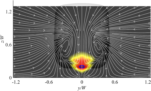
Figure 13: Structural sensitivity indicating sensitivity to mean flow modifications, the values are normalized by the maximum value; Streamlines are drawn based on mean flow; The blue line indicates normalized structural sensitivity = 0.90 isocontour.

In figure 13, the distribution of the structural sensitivity at the streamwise location where $\alpha^{+}$ and $\alpha^{-}$ branches intersect ($x/W=0.0731$) is shown. This field is obtained by first computing the adjoint mode on the considered cross-flow plane based on the methodology presented above and then calculating the $L^{2}$ norm of the sensitivity tensor following equation 36. In addition, mean flow streamlines are also included so that the structural sensitivity can be related to specific flow structures. Based on the results, both the upper and lower recirculation zones are highlighted. In particular, it can be observed that the position of the highest structural sensitivity, enclosed by the blue solid line in figure 13, is located slightly below the stagnation point of the recirculation region. The streamwise vortex pair generated from both sides of the train, on the other hand, seems to have no relevance to the sensitivity of the linear global mode. The highest structural sensitivity at this location, shown in figure 13, suggests that the interaction between the lower and upper shear layers, which drives the self-excitation of the instability, is the most sensitive to a steady external forcing and is therefore of significant importance in terms of controlling of the global mode. Note that in this part, a deeper interpretation of different components of the structural sensitivity tensor, as has been done in (Qadri et al., 2013), is beyond the scope of this work.

5 Comparison between empirical and theoretical modes

In this section, the near wake eigenmode which serves as the origin of the global mode, is tracked further downstream into the far wake to obtain the full picture of the linear global mode. The linear global mode is then compared with the leading SPOD mode to show the connections between them and to reveal additional physical driving mechanisms.

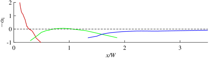
Figure 14: Spatial amplification rates of the most unstable near wake ( ), middle wake ( ) and far wake ( ) branches as functions of streamwise location, computed at the global complex frequency $\omega_{g}$.

To reconstruct the shape of the global mode, the $\alpha^{+}$ branch at $\omega_{\rm{g}}$ must be tracked in downstream direction reaching into the far wake. However, as illustrated in $\S$4.3, the complexity of the base flow gives rise to the problem that the physical eigenvalue may become highly stable at one location and fall into a spurious region, and then be untraceable at another location. Therefore, we do not only focus on the $\alpha^{+}$ branch, but also include spatial branches that arise and become unstable during the tracking process.

The results of the brnach tracking process are shown in figure 14. Accordingly, the near wake branch becomes spatially stable when approaching $x/W=0.3$, and cannot be tracked further downstream of $x/W=0.5$. However, at $x/W=0.4$, a new eigenmode, which corresponds to the middle wake branch, becomes the most spatially unstable. The middle wake branch develops to be slightly spatially unstable only within $0.75<x/W<1.05$, and remains spatially stable for most of the streamwise range of its occurrence. However, it is still the most unstable within the streamwise region $0.4<x/W<1.6$. Downstream of $x/W=1.6$, the far wake branch becomes dominant. The spatial amplification rate of the far wake eigenmode is observed to grow slightly upstream of $x/W=2.0$, then remains nearly constant with a marginally stable state after this location, which extends into the farthest streamwise location considered in this study.

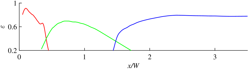
a

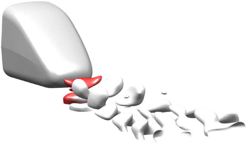
b

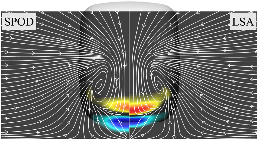
c

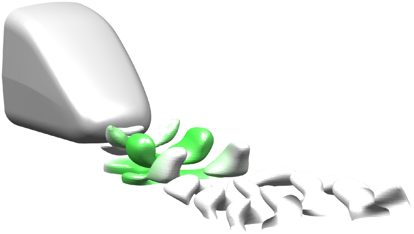
d

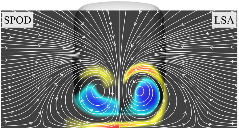
e

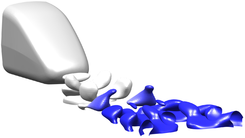
f

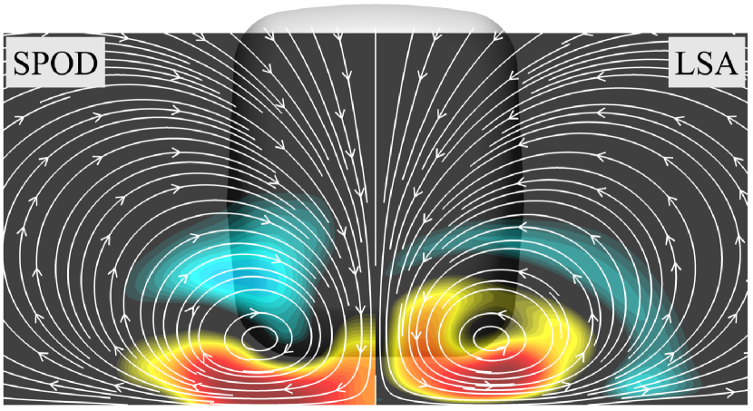
g

Figure 15: Comparison between the most dominated SPOD mode and the global linear stability mode from local analysis. (a) Alignment between the SPOD mode and the eigenmodes of the three branches (colors of lines correspond to figure 14) as functions of streamwise location; (b,d,f) The iso-surface of the streamwise component of SPOD mode colored respectively by the alignment with near wake, middle wake and far wake branches; (c,e,g) The streamwise component of the near wake, middle wake and far wake SPOD modes and eigenmodes.

To analyze whether these branches actually represent the empirical mode observed in the SPOD, we compute the alignment between the leading SPOD mode and the linear global mode based on the $L^{2}$ inner product. Since the wake flow is highly nonparallel, with several different spatial branches contributing to the linear global mode, we do not reconstruct the full three-dimensional global mode prior to the alignment measurement. Instead, the alignment between the leading SPOD mode and the three eigenmode branches are computed at all streamwise locations.

In figure 15(a), the alignment between the leading SPOD mode and the three eigenmode branches are plotted as a function of $x/W$. It can be observed that the alignment curves generally follow similar trends to the spatial growth rates of the three branches shown in figure 14, with the alignment value always being the highest for the most unstable eigenmode branch. In particular, the alignment is, in general, quite high with a value above 0.7, except for locations where the spatial branches switch. Therefore, the three eigenmode branches can be regarded as manifestations of the SPOD mode at different regions of the wake. This result further supports the modelling approach in this research for tracking the linear global mode in a highly complex three-dimensional base flow.

For better visualization, in figure 15(b,d,f), the three-dimensional SPOD mode is displayed based on the isosurface of the streamwise component, colored by the alignment of the three eigenmode branches. In addtion, figure 15(c,e,g) shows a direct comparisons between the cross-flow shapes of the SPOD mode and the linear global mode at different streamwise locations. In general, similar structures can be identified throughout the entire wake region. In the near wake region, the vortex shedding related to the transverse recirculation zone is dominant in both the SPOD and the linear global mode, with slightly different ranges between the two modes. Further downstream in the middle wake and far wake region, the coherent structures related to the streamwise vortex pair become dominant. The SPOD mode generally predicts a higher fluctuation amplitude near the ground and the central line, compared to the linear global mode.

In conclusion, the fundamental mechanism of instability in the considered flow problem can be interpreted as follows: Within the recirculation zone, the flow has a small region of absolute instability, which contributes to the global wavemaker located inside. The global frequency is well matched to the SPOD peak frequency and the linear global mode in this region has very high alignment with the SPOD mode. Further downstream, the flow becomes convectively unstable, amplifying the perturbations received by the global wavemaker, with the oscillation frequency synchronized to the global frequency. In this situation, the most spatially unstable branch becomes dominant and aligns the best with the SPOD mode.

6 Summary and Conclusions

Understanding important dynamics in complex technical flow is crucial in engineering practice. In this paper, three-dimensional coherent structures in the turbulent wake flow behind a generic high-speed train are investigated. A large eddy simulation has been performed to simulate and collect a database of the flow problem considered. For the purpose of this research, both the empirical identification approach based on SPOD and the theoretical approach using linear stability analysis are used.

The turbulent wake is found to be dominated by spanwise symmetric coherent structures, based on the comparison between the SPOD energy spectrum of symmetric and antisymmetric fluctuations. The most dominant SPOD mode is found to oscillate at the angular frequency of $\omega=3.437$. This dominant mode has an increasing wavelength in the near wake and a nearly constant wavelength in the far wake. The quadratic nonlinear interaction of the velocity perturbation is further checked by computing the mode bispectrum to explain the spectral distribution. The leading SPOD mode is identified with strong self-interaction, which generates the first-harmonic and subharmonic triads, meanwhile leading to significant deformation of the mean field. With the continuous evolution of this process, the flow finally appears to be low-rank in a wide frequency range.

The global instability is analyzed by employing a two-dimensional local spatio-temporal stability approach, following the WKBJ approximation and the weakly non-parallel flow assumption. Three spatial branches with positive temporal growth rate are found, with the near wake branch being the most unstable. The absolute frequency of the near wake branch is then found on the basis of a valid saddle point on the complex $\alpha^{+}$ plane and tracked along the streamwise direction. A confined region of absolute instability is identified in the near wake region. The global frequency is then determined to be $\omega_{\rm{g}}=3.2702+0.0797{\rm{i}}$ based on the frequency selection criterion, indicating a marginally stable global mode. This result is in excellent agreement with the empirical prediction in terms of angular frequency, and the theoretical expectation in terms of growth rate. The near wake recirculation zone is found to be related to the global mode wavemaker, which drives the self-excitation of the instability. The adjoint method is further used to compute the structural sensitivity at the location where the $\alpha^{+}$ and $\alpha^{-}$ branches intersect. In the corresponding cross-flow plane, the highest sensitivity is found near the upper and lower shear layers of the recirculation bubble, near the tip of the train nose. Accordingly, the global mode is expected to be most sensitive to mean flow changes in this region.

The linear global mode shape is further computed at each streamwise location by imposing the global frequency. Three spatial branches are found to be dominant respectively in the near, middle and far wake regions. The alignment between the linear global and leading SPOD modes is then performed to provide a quantitative comparison between mode shapes. Within the recirculation zone where the global wavemaker is located, the linear global mode has very high alignment with the SPOD mode. Further downstream, the flow becomes convectively unstable and the oscillations within these regions are synchronized with the global frequency by excitation from the wavemaker. Spatial branches with the highest spatial amplification rates become dominant and show highest alignment with the SPOD mode.

This work has two main conclusions, one methodological and one physical. Methodologically, a framework to track linear global mode in highly complex 3D base flows is introduced, and this method is justified a posteriori by the very good agreement with the empirical modes. To the authors’ knowledge, this is the first research dealing with the linear global stability in such a complex flow problem. Physically, the dominant SPOD mode is identified as being caused by a linear global mode in the wake of the train. This mode exhibits transverse symmetry and may cause significant fluctuations on the train surface, which can cause operational safety problems. The sensitivity analysis further shows that this mode could be quite effectively suppressed by small changes of the base flow near the tail of the train, which is of significant importance in terms of developing efficient flow control strategies.

Acknowledgements This work is supported by the National Science Foundation of China (grant no. 52202429), the Hunan Provincial Natural Science Foundation (grant no. 2023JJ40747) and the China Scholarship Council (grant no. 202006370204). The authors acknowledge the computational resources provided by the High Performance Computing Centre of Central South University, China.

Declaration of Interests The authors report no conflict of interest.

Appendix A Direct LSA operator

The operator matrices $\mathbf{\mathcal{A}}$ and $\mathbf{\mathcal{B}}$ used in the temporal stability analysis are shown as follows

$$\mathbf{\mathcal{A}}=\begin{bmatrix}\mathbf{\mathcal{C}}+\mathbf{\bar{u}}_{x}-\mathbf{\nu}_{tx}(\mathbf{\mathcal{D}}_{x}+{\rm{i}}\alpha)&\mathbf{\bar{u}}_{y}-\mathbf{\nu}_{ty}(\mathbf{\mathcal{D}}_{x}+{\rm{i}}\alpha)&\mathbf{\bar{u}}_{z}-\mathbf{\nu}_{tz}(\mathbf{\mathcal{D}}_{x}+{\rm{i}}\alpha)&\mathbf{\mathcal{D}}_{x}+{\rm{i}}\alpha\\ \mathbf{\bar{v}}_{x}-\mathbf{\nu}_{tx}\mathbf{\mathcal{D}}_{y}&\mathbf{\mathcal{C}}+\mathbf{\bar{v}}_{y}-\mathbf{\nu}_{ty}\mathbf{\mathcal{D}}_{y}&\mathbf{\bar{v}}_{z}-\mathbf{\nu}_{tz}\mathbf{\mathcal{D}}_{y}&\mathbf{\mathcal{D}}_{y}\\ \mathbf{\bar{w}}_{x}-\mathbf{\nu}_{tx}\mathbf{\mathcal{D}}_{z}&\mathbf{\bar{w}}_{y}-\mathbf{\nu}_{ty}\mathbf{\mathcal{D}}_{z}&\mathbf{\mathcal{C}}+\mathbf{\bar{w}}_{z}-\mathbf{\nu}_{tz}\mathbf{\mathcal{D}}_{z}&\mathbf{\mathcal{D}}_{z}\\ \mathbf{\mathcal{D}}_{x}+{\rm{i}}\alpha&\mathbf{\mathcal{D}}_{y}&\mathbf{\mathcal{D}}_{z}&{0}\end{bmatrix}$$ (43)

$$\mathbf{\mathcal{B}}=\begin{bmatrix}\rm{i}&{0}&{0}&{0}\\ {0}&\rm{i}&{0}&{0}\\ {0}&{0}&\rm{i}&{0}\\ {0}&{0}&{0}&{0}\end{bmatrix}$$ (44)

where subscripts $\left(.\right)_{x}$, $\left(.\right)_{y}$, and $\left(.\right)_{z}$ related to flow quantities denoting their first derivatives respect to the three directions, $\mathbf{\mathcal{D}}_{x}$, $\mathbf{\mathcal{D}}_{y}$ and $\mathbf{\mathcal{D}}_{z}$ are the first derivative matrices respect to the three directions. Operator $\mathbf{\mathcal{C}}$ can be written as

$$\mathbf{\mathcal{C}}= \mathbf{\bar{u}}(\mathbf{\mathcal{D}}_{x}+{\rm{i}}\alpha)+\mathbf{\bar{v}}\mathbf{\mathcal{D}}_{y}+\mathbf{\bar{w}}\mathbf{\mathcal{D}}_{z}-\left(\frac{1}{\mathit{Re}}+\mathbf{\nu}_{t}\right)(\mathbf{\mathcal{D}}_{yy}+\mathbf{\mathcal{D}}_{zz}+\mathbf{\mathcal{D}}_{xx}+2{\rm{i}}\alpha\mathbf{\mathcal{D}}_{x}-\alpha^{2})$$ (45)

$$-\mathbf{\nu}_{tx}(\mathbf{\mathcal{D}}_{x}+{\rm{i}}\alpha)-\mathbf{\nu}_{ty}\mathbf{\mathcal{D}}_{y}-\mathbf{\nu}_{tz}\mathbf{\mathcal{D}}_{z}$$

with $\mathbf{\mathcal{D}}_{xx}$, $\mathbf{\mathcal{D}}_{yy}$ and $\mathbf{\mathcal{D}}_{zz}$ being the second derivative matrices respect to the three directions.

In spatial stability analysis, operator matrices $\mathbf{\mathcal{A}}$ and $\mathbf{\mathcal{B}}$ take the form

$$\mathbf{\mathcal{A}}=\begin{bmatrix}\mathbf{\mathcal{C}}+\mathbf{\bar{u}}_{x}-\mathbf{\nu}_{tx}\mathbf{\mathcal{D}}_{x}&\mathbf{\bar{u}}_{y}-\mathbf{\nu}_{ty}\mathbf{\mathcal{D}}_{x}&\mathbf{\bar{u}}_{z}-\mathbf{\nu}_{tz}\mathbf{\mathcal{D}}_{x}&\mathbf{\mathcal{D}}_{x}&0&0&0\\ \mathbf{\bar{v}}_{x}-\mathbf{\nu}_{tx}\mathbf{\mathcal{D}}_{y}&\mathbf{\mathcal{C}}+\mathbf{\bar{v}}_{y}-\mathbf{\nu}_{ty}\mathbf{\mathcal{D}}_{y}&\mathbf{\bar{v}}_{z}-\mathbf{\nu}_{tz}\mathbf{\mathcal{D}}_{y}&\mathbf{\mathcal{D}}_{y}&0&0&0\\ \mathbf{\bar{w}}_{x}-\mathbf{\nu}_{tx}\mathbf{\mathcal{D}}_{z}&\mathbf{\bar{w}}_{y}-\mathbf{\nu}_{ty}\mathbf{\mathcal{D}}_{z}&\mathbf{\mathcal{C}}+\mathbf{\bar{w}}_{z}-\mathbf{\nu}_{tz}\mathbf{\mathcal{D}}_{z}&\mathbf{\mathcal{D}}_{z}&0&0&0\\ \mathbf{\mathcal{D}}_{x}&\mathbf{\mathcal{D}}_{y}&\mathbf{\mathcal{D}}_{z}&0&0&0&0\\ 0&0&0&0&1&0&0\\ 0&0&0&0&0&1&0\\ 0&0&0&0&0&0&1\\ \end{bmatrix}$$ (46)

$$\mathbf{\mathcal{B}}=\begin{bmatrix}\mathbf{\mathcal{E}}+{\rm{i}}\mathbf{\nu}_{tx}&{\rm{i}}\mathbf{\nu}_{ty}&{\rm{i}}\mathbf{\nu}_{tz}&-{\rm{i}}&-1/\mathit{Re}-\mathbf{\nu}_{t}&0&0\\ 0&\mathbf{\mathcal{E}}&0&0&0&-1/\mathit{Re}-\mathbf{\nu}_{t}&0\\ 0&0&\mathbf{\mathcal{E}}&0&0&0&-1/\mathit{Re}-\mathbf{\nu}_{t}\\ -{\rm{i}}&0&0&0&0&0&0\\ 1&0&0&0&0&0&0\\ 0&1&0&0&0&0&0\\ 0&0&1&0&0&0&0\\ \end{bmatrix}$$ (47)

with $\mathbf{\mathcal{C}}$ and $\mathbf{\mathcal{E}}$ being

$$\mathbf{\mathcal{C}}= -{\rm{i}}\omega+\mathbf{\bar{u}}\mathbf{\mathcal{D}}_{x}+\mathbf{\bar{v}}\mathbf{\mathcal{D}}_{y}+\mathbf{\bar{w}}\mathbf{\mathcal{D}}_{z}-\left(\frac{1}{\mathit{Re}}+\mathbf{\nu}_{t}\right)(\mathbf{\mathcal{D}}_{yy}+\mathbf{\mathcal{D}}_{zz}+\mathbf{\mathcal{D}}_{xx})$$ (48)

$$-\mathbf{\nu}_{tx}\mathbf{\mathcal{D}}_{x}-\mathbf{\nu}_{ty}\mathbf{\mathcal{D}}_{y}-\mathbf{\nu}_{tz}\mathbf{\mathcal{D}}_{z}$$

$$\mathbf{\mathcal{E}}=-{\rm{i}}\mathbf{\bar{u}}+2{\rm{i}}\left(\frac{1}{\mathit{Re}}+\mathbf{\nu}_{t}\right)\mathbf{\mathcal{D}}_{x}+{\rm{i}}\mathbf{\nu}_{tx}$$ (49)

Appendix B Adjoint LSA operator

The $x-$momentum equation is shown as an example of the derivation procedure. By premultiplying the equation by the adjoint eigenvector (equation 39), the left-hand side can be written as

$$\iint\left(\mathbf{\hat{u}^{\dagger}}\right)^{H}[-{\rm{i}}\omega+\mathbf{\bar{u}}(\mathbf{\mathcal{D}}_{x}+{\rm{i}}\alpha)+\mathbf{\bar{v}}\mathbf{\mathcal{D}}_{y}+\mathbf{\bar{w}}\mathbf{\mathcal{D}}_{z}-(1/\mathit{Re}+\mathbf{\nu}_{t})(\mathbf{\mathcal{D}}_{yy}+\mathbf{\mathcal{D}}_{zz}+\mathbf{\mathcal{D}}_{xx}+2{\rm{i}}\alpha\mathbf{\mathcal{D}}_{x}-\alpha^{2})$$ (50)

$$\ \ \ \ \ \ \ \ \ \ \ \ \ \ \ -\mathbf{\nu}_{tx}(\mathbf{\mathcal{D}}_{x}+{\rm{i}}\alpha)-\mathbf{\nu}_{ty}\mathbf{\mathcal{D}}_{y}-\mathbf{\nu}_{tz}\mathbf{\mathcal{D}}_{z}+\mathbf{\bar{u}}_{x}-\mathbf{\nu}_{tx}\mathbf{\mathcal{D}}_{x}-{\rm{i}}\alpha\mathbf{\nu}_{tx}]\left(\mathbf{\hat{u}}\right){\rm{d}}y{\rm{d}}z+$$

$$\iint\left(\mathbf{\hat{u}^{\dagger}}\right)^{H}\left(\mathbf{\bar{u}}_{y}-\mathbf{\nu}_{ty}\mathbf{\mathcal{D}}_{x}-{\rm{i}}\alpha\mathbf{\nu}_{ty}\right)\left(\mathbf{\hat{v}}\right){\rm{d}}y{\rm{d}}z+\iint\left(\mathbf{\hat{u}^{\dagger}}\right)^{H}\left(\mathbf{\bar{u}}_{z}-\mathbf{\nu}_{tz}\mathbf{\mathcal{D}}_{x}-{\rm{i}}\alpha\mathbf{\nu}_{tz}\right)\left(\mathbf{\hat{w}}\right){\rm{d}}y{\rm{d}}z+$$

$$\iint\left(\mathbf{\hat{u}^{\dagger}}\right)^{H}\left(\mathbf{\mathcal{D}}_{x}+{\rm{i}}\alpha\right)\left(\mathbf{\hat{p}}\right){\rm{d}}y{\rm{d}}z$$

We then present the integration-by-parts procedures for different types of terms in the equation for simplification. From a mathematical point of view, we can categorize terms in the equation based on whether they would have a derivative matrix acting on the state vector. For terms that do not have a derivative matrix acting on the state vector, we have

$$\iint\left(\mathbf{\hat{u}^{\dagger}}\right)^{H}\left[{\rm{i}}\alpha\mathbf{\bar{u}}\right]\left(\mathbf{\hat{u}}\right){\rm{d}}y{\rm{d}}z=\iint\left(-{\rm{i}}\alpha^{\ast}\mathbf{\bar{u}}\mathbf{\hat{u}^{\dagger}}\right)^{H}\left(\mathbf{\hat{u}}\right){\rm{d}}y{\rm{d}}z$$ (51)

If the first derivative matrix $\mathbf{\mathcal{D}}_{y}$ act on the state vector

$$\iint\left(\mathbf{\hat{u}^{\dagger}}\right)^{H}\left[\mathbf{\bar{v}}\mathbf{\mathcal{D}}_{y}\right]\left(\mathbf{\hat{u}}\right){\rm{d}}y{\rm{d}}z=-\iint\left(\mathbf{\mathcal{D}}_{y}\mathbf{\bar{v}}\mathbf{\hat{u}^{\dagger}}\right)^{H}\left(\mathbf{\hat{u}}\right){\rm{d}}y{\rm{d}}z+\oint\left(\mathbf{\bar{v}}\mathbf{\hat{u}^{\dagger}}\right)^{H}\left(\mathbf{\hat{u}}\right){\rm{d}}z$$ (52)

This procedure will leave boundary term which will have to be canceled then. Also for $\mathbf{\mathcal{D}}_{z}$

$$\iint\left(\mathbf{\hat{u}^{\dagger}}\right)^{H}\left[\mathbf{\bar{w}}\mathbf{\mathcal{D}}_{z}\right]\left(\mathbf{\hat{u}}\right){\rm{d}}y{\rm{d}}z=-\iint\left(\mathbf{\mathcal{D}}_{z}\mathbf{\bar{w}}\mathbf{\hat{u}^{\dagger}}\right)^{H}\left(\mathbf{\hat{u}}\right){\rm{d}}y{\rm{d}}z-\oint\left(\mathbf{\bar{w}}\mathbf{\hat{u}^{\dagger}}\right)^{H}\left(\mathbf{\hat{u}}\right){\rm{d}}y$$ (53)

For $\mathbf{\mathcal{D}}_{x}$, as this operator assume an artificial $x-$derivative, the form $\mathbf{\mathcal{D}}_{x}=-{\rm{tan}}\mathbf{\theta}\mathbf{\mathcal{D}}_{y}-{\rm{tan}}\mathbf{\gamma}\mathbf{\mathcal{D}}_{z}$ has to be taken back for the integration-by-parts procedure. Here for simplification, we refer $\mathbf{a}=-{\rm{tan}}\mathbf{\theta}$ and $\mathbf{b}=-{\rm{tan}}\mathbf{\gamma}$. Then we have

$$\iint\left(\mathbf{\hat{u}^{\dagger}}\right)^{H}\left[\mathbf{\bar{u}}\mathbf{\mathcal{D}}_{x}\right]\left(\mathbf{\hat{u}}\right){\rm{d}}y{\rm{d}}z=\iint\left(\mathbf{\hat{u}^{\dagger}}\right)^{H}\left[\mathbf{\bar{u}}\mathbf{a}\mathbf{\mathcal{D}}_{y}+\mathbf{\bar{u}}\mathbf{b}\mathbf{\mathcal{D}}_{z}\right]\left(\mathbf{\hat{u}}\right){\rm{d}}y{\rm{d}}z$$ (54)

$$= -\iint\left[\left(\mathbf{\mathcal{D}}_{y}\mathbf{a}\mathbf{\bar{u}}+\mathbf{\mathcal{D}}_{z}\mathbf{b}\mathbf{\bar{u}}\right)\mathbf{\hat{u}^{\dagger}}\right]^{H}\left(\mathbf{\hat{u}}\right){\rm{d}}y{\rm{d}}z+\oint\left(\mathbf{a}\mathbf{\bar{u}}\mathbf{\hat{u}^{\dagger}}\right)^{H}\left(\mathbf{\hat{u}}\right){\rm{d}}z-\oint\left(\mathbf{b}\mathbf{\bar{u}}\mathbf{\hat{u}^{\dagger}}\right)^{H}\left(\mathbf{\hat{u}}\right){\rm{d}}y$$

Similarly, for all second derivative matrices

$$\iint\left(\mathbf{\hat{u}^{\dagger}}\right)^{H}\left[\mathbf{\nu}_{t}\mathbf{\mathcal{D}}_{yy}\right]\left(\mathbf{\hat{u}}\right){\rm{d}}y{\rm{d}}z=\iint\left(\mathbf{\mathcal{D}}_{yy}\mathbf{\nu}_{t}\mathbf{\hat{u}^{\dagger}}\right)^{H}\left(\mathbf{\hat{u}}\right){\rm{d}}y{\rm{d}}z+\oint\left[\left(\mathbf{\nu}_{t}\mathbf{\hat{u}^{\dagger}}\right)^{H}\left(\mathbf{\mathcal{D}}_{y}\mathbf{\hat{u}}\right)-\left(\mathbf{\mathcal{D}}_{y}\mathbf{\nu}_{t}\mathbf{\hat{u}^{\dagger}}\right)^{H}\left(\mathbf{\hat{u}}\right)\right]{\rm{d}}z$$ (55)

$$\iint\left(\mathbf{\hat{u}^{\dagger}}\right)^{H}\left[\mathbf{\nu}_{t}\mathbf{\mathcal{D}}_{zz}\right]\left(\mathbf{\hat{u}}\right){\rm{d}}y{\rm{d}}z=\iint\left(\mathbf{\mathcal{D}}_{zz}\mathbf{\nu}_{t}\mathbf{\hat{u}^{\dagger}}\right)^{H}\left(\mathbf{\hat{u}}\right){\rm{d}}y{\rm{d}}z-\oint\left[\left(\mathbf{\nu}_{t}\mathbf{\hat{u}^{\dagger}}\right)^{H}\left(\mathbf{\mathcal{D}}_{z}\mathbf{\hat{u}}\right)-\left(\mathbf{\mathcal{D}}_{z}\mathbf{\nu}_{t}\mathbf{\hat{u}^{\dagger}}\right)^{H}\left(\mathbf{\hat{u}}\right)\right]{\rm{d}}y$$ (56)

$$\iint\left(\mathbf{\hat{u}^{\dagger}}\right)^{H}\left[\mathbf{\nu}_{t}\mathbf{\mathcal{D}}_{xx}\right]\left(\mathbf{\hat{u}}\right){\rm{d}}y{\rm{d}}z=\iint\left(\mathbf{\hat{u}^{\dagger}}\right)^{H}\left[\mathbf{\nu}_{t}\mathbf{a}^{2}\mathbf{\mathcal{D}}_{yy}+2\mathbf{\nu}_{t}\mathbf{ab}\mathbf{\mathcal{D}}_{y}\mathbf{\mathcal{D}}_{z}+\mathbf{\nu}_{t}\mathbf{b}^{2}\mathbf{\mathcal{D}}_{zz}\right]\left(\mathbf{\hat{u}}\right){\rm{d}}y{\rm{d}}z$$ (57)

$$= \iint\left[\left(\mathbf{\mathcal{D}}_{yy}\mathbf{a}^{2}\mathbf{\nu}_{t}+2\mathbf{\mathcal{D}}_{y}\mathbf{\mathcal{D}}_{z}\mathbf{ab}\mathbf{\nu}_{t}+\mathbf{\mathcal{D}}_{zz}\mathbf{b}^{2}\mathbf{\nu}_{t}\right)\mathbf{\hat{u}^{\dagger}}\right]^{H}\left(\mathbf{\hat{u}}\right){\rm{d}}y{\rm{d}}z+$$

$$\oint\left[\left(\mathbf{a}^{2}\mathbf{\nu}_{t}\mathbf{\hat{u}^{\dagger}}\right)^{H}\left(\mathbf{\mathcal{D}}_{y}\mathbf{\hat{u}}\right)-\left(\mathbf{\mathcal{D}}_{y}\mathbf{a}^{2}\mathbf{\nu}_{t}\mathbf{\hat{u}^{\dagger}}\right)^{H}\left(\mathbf{\hat{u}}\right)+2\left(\mathbf{ab}\mathbf{\nu}_{t}\mathbf{\hat{u}^{\dagger}}\right)^{H}\left(\mathbf{\mathcal{D}}_{z}\mathbf{\hat{u}}\right)\right]{\rm{d}}z-$$

$$\oint\left[\left(\mathbf{b}^{2}\mathbf{\nu}_{t}\mathbf{\hat{u}^{\dagger}}\right)^{H}\left(\mathbf{\mathcal{D}}_{z}\mathbf{\hat{u}}\right)-\left(\mathbf{\mathcal{D}}_{z}\mathbf{b}^{2}\mathbf{\nu}_{t}\mathbf{\hat{u}^{\dagger}}\right)^{H}\left(\mathbf{\hat{u}}\right)-2\left(\mathbf{\mathcal{D}}_{y}\mathbf{ab}\mathbf{\nu}_{t}\mathbf{\hat{u}^{\dagger}}\right)^{H}\left(\mathbf{\hat{u}}\right)\right]{\rm{d}}y$$

By applying these procedures to all terms in equation 50 and rearranging, the adjoint operators $\mathbf{\mathcal{A}^{\dagger}}$ and $\mathbf{\mathcal{B}^{\dagger}}$ can be written as

$$\hskip-14.22636pt\mathbf{\mathcal{A}^{\dagger}}=\begin{bmatrix}\mathbf{\mathcal{C}^{\dagger}}+\mathbf{\bar{u}}_{x}+(\mathbf{\mathcal{D}}_{y}\mathbf{a}+\mathbf{\mathcal{D}}_{z}\mathbf{b})\mathbf{\nu}_{tx}&\mathbf{\bar{v}}_{x}+\mathbf{\mathcal{D}}_{y}\mathbf{\nu}_{tx}&\mathbf{\bar{w}}_{x}+\mathbf{\mathcal{D}}_{z}\mathbf{\nu}_{tx}&-\mathbf{\mathcal{D}}_{y}\mathbf{a}-\mathbf{\mathcal{D}}_{z}\mathbf{b}&0&0&0\\ \mathbf{\bar{u}}_{y}+(\mathbf{\mathcal{D}}_{y}\mathbf{a}+\mathbf{\mathcal{D}}_{z}\mathbf{b})\mathbf{\nu}_{ty}&\mathbf{\mathcal{C}^{\dagger}}+\mathbf{\bar{v}}_{y}+\mathbf{\mathcal{D}}_{y}\mathbf{\nu}_{ty}&\mathbf{\bar{w}}_{y}+\mathbf{\mathcal{D}}_{z}\mathbf{\nu}_{ty}&-\mathbf{\mathcal{D}}_{y}&0&0&0\\ \mathbf{\bar{u}}_{z}+(\mathbf{\mathcal{D}}_{y}\mathbf{a}+\mathbf{\mathcal{D}}_{z}\mathbf{b})\mathbf{\nu}_{tz}&\mathbf{\bar{v}}_{z}+\mathbf{\mathcal{D}}_{y}\mathbf{\nu}_{tz}&\mathbf{\mathcal{C}^{\dagger}}+\mathbf{\bar{w}}_{z}+\mathbf{\mathcal{D}}_{z}\mathbf{\nu}_{tz}&-\mathbf{\mathcal{D}}_{z}&0&0&0\\ -\mathbf{\mathcal{D}}_{y}\mathbf{a}-\mathbf{\mathcal{D}}_{z}\mathbf{b}&-\mathbf{\mathcal{D}}_{y}&-\mathbf{\mathcal{D}}_{z}&0&0&0&0\\ 0&0&0&0&1&0&0\\ 0&0&0&0&0&1&0\\ 0&0&0&0&0&0&1\\ \end{bmatrix}$$ (58)

$$\mathbf{\mathcal{B}^{\dagger}}=\begin{bmatrix}\mathbf{\mathcal{E}^{\dagger}}-{\rm{i}}\mathbf{\nu}_{tx}&0&0&{\rm{i}}&-1/\mathit{Re}-\mathbf{\nu}_{t}&0&0\\ -{\rm{i}}\mathbf{\nu}_{ty}&\mathbf{\mathcal{E}^{\dagger}}&0&0&0&-1/\mathit{Re}-\mathbf{\nu}_{t}&0\\ -{\rm{i}}\mathbf{\nu}_{tz}&0&\mathbf{\mathcal{E}^{\dagger}}&0&0&0&-1/\mathit{Re}-\mathbf{\nu}_{t}\\ {\rm{i}}&0&0&0&0&0&0\\ 1&0&0&0&0&0&0\\ 0&1&0&0&0&0&0\\ 0&0&1&0&0&0&0\\ \end{bmatrix}$$ (59)

with $\mathbf{\mathcal{C}^{\dagger}}$ and $\mathbf{\mathcal{E}^{\dagger}}$ given the form

$$\mathbf{\mathcal{C}^{\dagger}}= {\rm{i}}\omega^{\ast}-\mathbf{\mathcal{D}}_{y}\mathbf{a}\mathbf{\bar{u}}-\mathbf{\mathcal{D}}_{z}\mathbf{b}\mathbf{\bar{u}}-\mathbf{\mathcal{D}}_{y}\mathbf{\bar{v}}-\mathbf{\mathcal{D}}_{z}\mathbf{\bar{w}}-\mathbf{\mathcal{D}}_{yy}\left(\frac{1}{\mathit{Re}}+\mathbf{\nu}_{t}\right)-\mathbf{\mathcal{D}}_{zz}\left(\frac{1}{\mathit{Re}}+\mathbf{\nu}_{t}\right)$$ (60)

$$-\left(\mathbf{\mathcal{D}}_{yy}\mathbf{a}^{2}+2\mathbf{\mathcal{D}}_{y}\mathbf{\mathcal{D}}_{z}\mathbf{ab}+\mathbf{\mathcal{D}}_{zz}\mathbf{b}^{2}\right)\left(\frac{1}{\mathit{Re}}+\mathbf{\nu}_{t}\right)+\mathbf{\mathcal{D}}_{y}\mathbf{a}\mathbf{\nu}_{tx}+\mathbf{\mathcal{D}}_{z}\mathbf{b}\mathbf{\nu}_{tx}$$

$$+\mathbf{\mathcal{D}}_{y}\mathbf{\nu}_{ty}+\mathbf{\mathcal{D}}_{z}\mathbf{\nu}_{tz}$$

$$\mathbf{\mathcal{E}^{\dagger}}={\rm{i}}\mathbf{\bar{u}}+2{\rm{i}}(\mathbf{\mathcal{D}}_{y}\mathbf{a}+\mathbf{\mathcal{D}}_{z}\mathbf{b})\left(\frac{1}{\mathit{Re}}+\mathbf{\nu}_{t}\right)-{\rm{i}}\mathbf{\nu}_{tx}$$ (61)

The boundary terms should then be canceled by applying appropriate adjoint boundary conditions. The expression for boundary terms on side boundaries is

$$\hskip-14.22636pt\oint\left(\mathbf{a}\mathbf{\bar{u}}\mathbf{\hat{u}^{\dagger}}\right)^{H}\mathbf{\hat{u}}{\rm{d}}z+\oint\left(\mathbf{\bar{v}}\mathbf{\hat{u}^{\dagger}}\right)^{H}\mathbf{\hat{u}}{\rm{d}}z-\oint\left[\left(\left(\frac{1}{\mathit{Re}}+\mathbf{\nu}_{t}\right)\mathbf{\hat{u}^{\dagger}}\right)^{H}\mathbf{\mathcal{D}}_{y}\mathbf{\hat{u}}-\left(\mathbf{\mathcal{D}}_{y}\left(\frac{1}{\mathit{Re}}+\mathbf{\nu}_{t}\right)\mathbf{\hat{u}^{\dagger}}\right)^{H}\mathbf{\hat{u}}\right]{\rm{d}}z-$$ (62)

$$\hskip-14.22636pt\oint\left[\left(\mathbf{a}^{2}\left(\frac{1}{\mathit{Re}}+\mathbf{\nu}_{t}\right)\mathbf{\hat{u}^{\dagger}}\right)^{H}\mathbf{\mathcal{D}}_{y}\mathbf{\hat{u}}-\left(\mathbf{\mathcal{D}}_{y}\mathbf{a}^{2}\left(\frac{1}{\mathit{Re}}+\mathbf{\nu}_{t}\right)\mathbf{\hat{u}^{\dagger}}\right)^{H}\mathbf{\hat{u}}+2\left(\mathbf{ab}\left(\frac{1}{\mathit{Re}}+\mathbf{\nu}_{t}\right)\mathbf{\hat{u}^{\dagger}}\right)^{H}\mathbf{\mathcal{D}}_{z}\mathbf{\hat{u}}\right]{\rm{d}}z-$$

$$\hskip-14.22636pt2{\rm{i}}\alpha^{\ast}\oint\left(\mathbf{a}\mathbf{\hat{u}^{\dagger}}\right)^{H}\mathbf{\hat{u}}{\rm{d}}z-\oint\left(\mathbf{a}\mathbf{\nu}_{tx}\mathbf{\hat{u}^{\dagger}}\right)^{H}\mathbf{\hat{u}}{\rm{d}}z-\oint\left(\mathbf{\nu}_{ty}\mathbf{\hat{u}^{\dagger}}\right)^{H}\mathbf{\hat{u}}{\rm{d}}z-\oint\left(\mathbf{a}\mathbf{\nu}_{tx}\mathbf{\hat{u}^{\dagger}}\right)^{H}\mathbf{\hat{u}}{\rm{d}}z-$$

$$\hskip-14.22636pt\oint\left(\mathbf{a}\mathbf{\nu}_{ty}\mathbf{\hat{u}^{\dagger}}\right)^{H}\mathbf{\hat{v}}{\rm{d}}z-\oint\left(\mathbf{a}\mathbf{\nu}_{tz}\mathbf{\hat{u}^{\dagger}}\right)^{H}\mathbf{\hat{w}}{\rm{d}}z+\oint\left(\mathbf{a}\mathbf{\hat{u}^{\dagger}}\right)^{H}\mathbf{\hat{p}}{\rm{d}}z$$

and on vertical boundaries is

$$\hskip-14.22636pt-\oint\left(\mathbf{b}\mathbf{\bar{u}}\mathbf{\hat{u}^{\dagger}}\right)^{H}\mathbf{\hat{u}}{\rm{d}}y-\oint\left(\mathbf{\bar{w}}\mathbf{\hat{u}^{\dagger}}\right)^{H}\mathbf{\hat{u}}{\rm{d}}y+\oint\left[\left(\left(\frac{1}{\mathit{Re}}+\mathbf{\nu}_{t}\right)\mathbf{\hat{u}^{\dagger}}\right)^{H}\mathbf{\mathcal{D}}_{z}\mathbf{\hat{u}}-\left(\mathbf{\mathcal{D}}_{z}\left(\frac{1}{\mathit{Re}}+\mathbf{\nu}_{t}\right)\mathbf{\hat{u}^{\dagger}}\right)^{H}\mathbf{\hat{u}}\right]{\rm{d}}y+$$ (63)

$$\hskip-14.22636pt\oint\left[\left(\mathbf{b}^{2}\left(\frac{1}{\mathit{Re}}+\mathbf{\nu}_{t}\right)\mathbf{\hat{u}^{\dagger}}\right)^{H}\mathbf{\mathcal{D}}_{z}\mathbf{\hat{u}}-\left(\mathbf{\mathcal{D}}_{z}\mathbf{b}^{2}\left(\frac{1}{\mathit{Re}}+\mathbf{\nu}_{t}\right)\mathbf{\hat{u}^{\dagger}}\right)^{H}\mathbf{\hat{u}}-2\left(\mathbf{\mathcal{D}}_{y}\mathbf{ab}\left(\frac{1}{\mathit{Re}}+\mathbf{\nu}_{t}\right)\mathbf{\hat{u}^{\dagger}}\right)^{H}\mathbf{\hat{u}}\right]{\rm{d}}y+$$

$$\hskip-14.22636pt2{\rm{i}}\alpha^{\ast}\oint\left(\mathbf{b}\mathbf{\hat{u}^{\dagger}}\right)^{H}\mathbf{\hat{u}}{\rm{d}}y+\oint\left(\mathbf{b}\mathbf{\nu}_{tx}\mathbf{\hat{u}^{\dagger}}\right)^{H}\mathbf{\hat{u}}{\rm{d}}y+\oint\left(\mathbf{\nu}_{tz}\mathbf{\hat{u}^{\dagger}}\right)^{H}\mathbf{\hat{u}}{\rm{d}}y+\oint\left(\mathbf{b}\mathbf{\nu}_{tx}\mathbf{\hat{u}^{\dagger}}\right)^{H}\mathbf{\hat{u}}{\rm{d}}y+$$

$$\hskip-14.22636pt\oint\left(\mathbf{b}\mathbf{\nu}_{ty}\mathbf{\hat{u}^{\dagger}}\right)^{H}\mathbf{\hat{v}}{\rm{d}}y+\oint\left(\mathbf{b}\mathbf{\nu}_{tz}\mathbf{\hat{u}^{\dagger}}\right)^{H}\mathbf{\hat{w}}{\rm{d}}y-\oint\left(\mathbf{b}\mathbf{\hat{u}^{\dagger}}\right)^{H}\mathbf{\hat{p}}{\rm{d}}y$$

Although these expressions are given in a huge form, they can be converted into much simpler forms, since the adjoint mode only needs to be computed in the near wake region. Therefore we can consider all direct and adjoint perturbations on the far-field boundary to be zero, then only the boundary terms on $y/W=0$ and $z/W=0$ should be further considered. On $y/W=0$ we have the following conditions and equation 62 can be simplified into

$$\mathbf{a}=\mathbf{\bar{v}}=\mathbf{\nu}_{ty}=\mathbf{\hat{u}}_{y}=0\ {\rm{on}}\ y/W=0$$ (64a)

$$\oint\left[\left(\frac{1}{\mathit{Re}}+\mathbf{\nu}_{t}\right)\mathbf{\mathcal{D}}_{y}\mathbf{\hat{u}^{\dagger}}\right]^{H}\mathbf{\hat{u}}{\rm{d}}z$$ (64b)

and on $z/W=0$ these conditions can be applied with equation 63 can be simplified into

$$\mathbf{b}=\mathbf{\bar{w}}=\mathbf{\hat{u}}=0\ {\rm{on}}\ z/W=0$$ (65a)

$$\oint\left[\left(\frac{1}{\mathit{Re}}+\mathbf{\nu}_{t}\right)\mathbf{\hat{u}^{\dagger}}\right]^{H}\mathbf{\mathcal{D}}_{z}\mathbf{\hat{u}}{\rm{d}}z$$ (65b)

Therefore all adjoint boundary conditions appropriate to cancel the boundary terms are summarized as follows

$$\frac{\partial{\mathbf{\hat{u}^{\dagger}}}}{\partial{y}}=\frac{\partial{\mathbf{\hat{w}^{\dagger}}}}{\partial{y}}=\frac{\partial{\mathbf{\hat{p}^{\dagger}}}}{\partial{y}}=0,\mathbf{\hat{v}^{\dagger}}=0\ {\rm{on}}\ y/W=0$$ (66a)

$$\mathbf{\hat{u}^{\dagger}}=\mathbf{\hat{v}^{\dagger}}=\mathbf{\hat{w}^{\dagger}}=\mathbf{\hat{p}^{\dagger}}=0\ {\rm{on}}\ y/W=1.3$$ (66b)

$$\mathbf{\hat{u}^{\dagger}}=\mathbf{\hat{v}^{\dagger}}=\mathbf{\hat{w}^{\dagger}}=0,\frac{\partial{\mathbf{\hat{p}^{\dagger}}}}{\partial{z}}=0\ {\rm{on}}\ z/W=0$$ (66c)

$$\mathbf{\hat{u}^{\dagger}}=\mathbf{\hat{v}^{\dagger}}=\mathbf{\hat{w}^{\dagger}}=\mathbf{\hat{p}^{\dagger}}=0\ {\rm{on}}\ z/W=1.3$$ (66d)

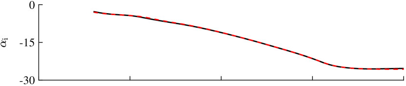
a

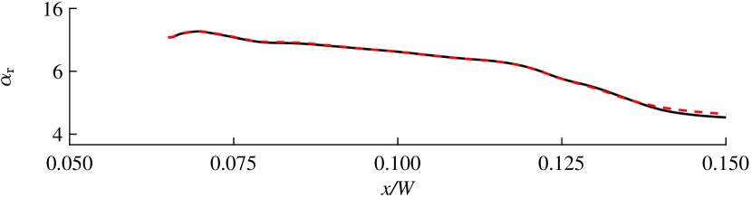
b

Figure 16: Local complex streamwise wavenumber of the adjoint mode based on direct LNS equation (black solid line), and its complex conjugation based on adjoint LNS equation (red dashed line). (a) The real component; (b) The imaginary component.

To validate the adjoint operators and boundary conditions, we take the conjugation of the complex streamwise wavenumber of the adjoint mode computed based on the adjoint method and compare it with the results from the direct approach, as shown in figure 12(e,f). The comparisons are shown in figure 16. Good agreement can be observed between the two approaches, with discrepancies being observed only downstream of $x/W=0.135$. This is due to the fact that, downstream of this streamwise location, the adjoint eigenvalue is quite far from the real axis, which would lead to a convergence issue of the eigenvalue problem. At locations around the wavemaker regions, the two lines are almost identical, which confirms that the adjoint operators and boundary conditions presented in this paper should provide with accurate prediction on the adjoint mode and subsequently structural sensitivity.

References

- Abreu et al. (2020) Abreu, L. I., Cavalieri, A. V. G., Schlatter, P., Vinuesa, R. & Henningson, D. S. 2020 Spectral proper orthogonal decomposition and resolvent analysis of near-wall coherent structures in turbulent pipe flows. Journal of Fluid Mechanics 900, A11.
- Abreu et al. (2021) Abreu, L. I., Tanarro, A., Cavalieri, A. V.G., Schlatter, P., Vinuesa, R., Hanifi, A. & Henningson, D. S. 2021 Spanwise-coherent hydrodynamic waves around flat plates and airfoils. Journal of Fluid Mechanics 927, A1.
- Ahmed et al. (1984) Ahmed, S. R., Ramm, G. & Faltin, G. 1984 Some salient features of the time-averaged ground vehicle wake. SAE transactions pp. 473–503.
- Barkley (2006) Barkley, D. 2006 Linear analysis of the cylinder wake mean flow. Europhysics Letters 75 (5), 750.
- Blanco et al. (2022) Blanco, D. C.P., Martini, E., Sasaki, K. & Cavalieri, A. V.G. 2022 Improved convergence of the spectral proper orthogonal decomposition through time shifting. Journal of Fluid Mechanics 950, A9.
- Bridges & Morris (1984) Bridges, T.J. & Morris, P.J. 1984 Differential eigenvalue problems in which the parameter appears nonlinearly. Journal of Computational Physics 55 (3), 437–460.
- Briggs (1964) Briggs, R. J. 1964 Electron-stream interaction with plasmas. Electron-stream interaction with plasmas .
- Casel et al. (2022) Casel, M., Oberleithner, K., Zhang, F.-C., Zirwes, T., Bockhorn, H., Trimis, D. & Kaiser, T. L. 2022 Resolvent-based modelling of coherent structures in a turbulent jet flame using a passive flame approach. Combustion and Flame 236, 111695.
- Chandler et al. (2012) Chandler, G. J., Juniper, M. P., Nichols, J. W. & Schmid, P. J. 2012 Adjoint algorithms for the navier–stokes equations in the low mach number limit. Journal of Computational Physics 231 (4), 1900–1916.
- Chomaz (2005) Chomaz, J.-M. 2005 Global instabilities in spatially developing flows: non-normality and nonlinearity. Annu. Rev. Fluid Mech. 37, 357–392.
- Chomaz et al. (1991) Chomaz, J.-M., Huerre, P. & Redekopp, L. G. 1991 A frequency selection criterion in spatially developing flows. Studies in applied mathematics 84 (2), 119–144.
- Colonius et al. (2002) Colonius, T., Rowley, C. W., Freund, J. B. & Murray, R. M. 2002 On the choice of norm for modeling compressible flow dynamics at reduced-order using the pod. In Proceedings of the 41st IEEE Conference on Decision and Control, 2002., , vol. 3, pp. 3273–3278 vol.3.
- Cooper & Crighton (2000) Cooper, A. J. & Crighton, D. G. 2000 Global modes and superdirective acoustic radiation in low-speed axisymmetric jets. European Journal of Mechanics-B/Fluids 19 (5), 559–574.
- Demange et al. (2020) Demange, S., Chazot, O. & Pinna, F. 2020 Local analysis of absolute instability in plasma jets. Journal of Fluid Mechanics 903, A51.
- Demange et al. (2022) Demange, S., Qadri, U. A., Juniper, M. P. & Pinna, F. 2022 Global modes of viscous heated jets with real gas effects. Journal of Fluid Mechanics 936, A7.
- Evstafyeva et al. (2017) Evstafyeva, O., Morgans, A. S. & Dalla Longa, L. 2017 Simulation and feedback control of the ahmed body flow exhibiting symmetry breaking behaviour. Journal of Fluid Mechanics 817, R2.
- Giannetti & Luchini (2007) Giannetti, F. & Luchini, P. 2007 Structural sensitivity of the first instability of the cylinder wake. Journal of Fluid Mechanics 581, 167–197.
- Gómez et al. (2014) Gómez, F., Gómez, R. & Theofilis, V. 2014 On three-dimensional global linear instability analysis of flows with standard aerodynamics codes. Aerospace Science and Technology 32 (1), 223–234.
- Grandemange et al. (2013) Grandemange, M., Gohlke, M. & Cadot, O. 2013 Turbulent wake past a three-dimensional blunt body. part 1. global modes and bi-stability. Journal of Fluid Mechanics 722, 51–84.
- Grandemange et al. (2014) Grandemange, M., Gohlke, M. & Cadot, O. 2014 Turbulent wake past a three-dimensional blunt body. part 2. experimental sensitivity analysis. Journal of Fluid Mechanics 752, 439–461.
- Hack & Schmidt (2021) Hack, M. J. P. & Schmidt, O. T. 2021 Extreme events in wall turbulence. Journal of Fluid Mechanics 907, A9.
- Haffner et al. (2020) Haffner, Y., Borée, J., Spohn, A. & Castelain, T. 2020 Mechanics of bluff body drag reduction during transient near-wake reversals. Journal of Fluid Mechanics 894, A14.
- He et al. (2021a) He, K., Minelli, G., Wang, J.-B., Dong, T.-Y., Gao, G.-J. & Krajnović, S. 2021a Numerical investigation of the wake bi-stability behind a notchback ahmed body. Journal of Fluid Mechanics 926, A36.
- He et al. (2021b) He, X., Fang, Z., Rigas, G. & Vahdati, M. 2021b Spectral proper orthogonal decomposition of compressor tip leakage flow. Physics of Fluids 33 (10).
- Huerre & Monkewitz (1990) Huerre, P. & Monkewitz, P. A. 1990 Local and global instabilities in spatially developing flows. Annual review of fluid mechanics 22 (1), 473–537.
- Juniper et al. (2014) Juniper, M. P., Hanifi, A. & Theofilis, V. 2014 Modal stability theorylecture notes from the flow-nordita summer school on advanced instability methods for complex flows, stockholm, sweden, 2013. Applied Mechanics Reviews 66 (2).
- Juniper & Pier (2015) Juniper, M. P. & Pier, B. 2015 The structural sensitivity of open shear flows calculated with a local stability analysis. European Journal of Mechanics - B/Fluids 49, 426–437.
- Juniper et al. (2011) Juniper, M. P., Tammisola, O. & Lundell, F. 2011 The local and global stability of confined planar wakes at intermediate reynolds number. Journal of Fluid Mechanics 686, 218–238.
- Kaiser et al. (2018) Kaiser, T. L., Poinsot, T. & Oberleithner, K. 2018 Stability and Sensitivity Analysis of Hydrodynamic Instabilities in Industrial Swirled Injection Systems. Journal of Engineering for Gas Turbines and Power 140 (5), 051506.
- Khorrami (1991) Khorrami, M. R. 1991 On the viscous modes of instability of a trailing line vortex. Journal of Fluid Mechanics 225, 197–212.
- Khorrami et al. (1989) Khorrami, M. R., Malik, M. R. & Ash, R. L. 1989 Application of spectral collocation techniques to the stability of swirling flows. Journal of Computational Physics 81 (1), 206–229.
- Kuhn et al. (2021) Kuhn, P., Soria, J. & Oberleithner, K. 2021 Linear modelling of self-similar jet turbulence. Journal of Fluid Mechanics 919, A7.
- Kurz & Kloker (2016) Kurz, H. B. E. & Kloker, M. J. 2016 Mechanisms of flow tripping by discrete roughness elements in a swept-wing boundary layer. Journal of Fluid Mechanics 796, 158–194.
- Li et al. (2021a) Li, X.-B., Chen, G., Liang, X.-F., Liu, D.-R. & Xiong, X.-H. 2021a Research on spectral estimation parameters for application of spectral proper orthogonal decomposition in train wake flows. Physics of Fluids 33 (12), 125103.
- Li et al. (2021b) Li, X.-B., Liang, X.-F., Wang, Z., Xiong, X.-H., Chen, G., Yu, Y.-Z. & Chen, C.-M. 2021b On the correlation between aerodynamic drag and wake flow for a generic high-speed train. Journal of Wind Engineering and Industrial Aerodynamics 215, 104698.
- Li et al. (2022) Li, Y.-Q., Cui, W.-S., Jia, Q., Li, Q.-L., Yang, Z.-G., Morzyński, M. & Noack, B. R. 2022 Explorative gradient method for active drag reduction of the fluidic pinball and slanted ahmed body. Journal of Fluid Mechanics 932, A7.
- Lienhart et al. (2002) Lienhart, H., Stoots, C. & Becker, S. 2002 Flow and turbulence structures in the wake of a simplified car model (ahmed modell). In New Results in Numerical and Experimental Fluid Mechanics III: Contributions to the 12th STAB/DGLR Symposium Stuttgart, Germany 2000, pp. 323–330. Springer.
- Liu et al. (2016) Liu, C.-Q., Wang, Y.-Q., Yang, Y. & Duan, Z.-W 2016 New omega vortex identification method. Science China 59 (8), 684711.
- Liu et al. (2021) Liu, K., Zhang, B.-F., Zhang, Y.-C. & Zhou, Y. 2021 Flow structure around a low-drag ahmed body. Journal of Fluid Mechanics 913, A21.
- Loiseau et al. (2014) Loiseau, J.-C., Robinet, J.-C., Cherubini, S. & Leriche, E. 2014 Investigation of the roughness-induced transition: global stability analyses and direct numerical simulations. Journal of Fluid Mechanics 760, 175–211.
- Lumley (1967) Lumley, J. L. 1967 The structure of inhomogeneous turbulent flows. Atmospheric turbulence and radio wave propagation pp. 166–178.
- Lumley (1970) Lumley, J. L. 1970 Stochastic tools in turbulence. Academic Press.
- Ma & Mahesh (2022) Ma, R. & Mahesh, K. 2022 Global stability analysis and direct numerical simulation of boundary layers with an isolated roughness element. Journal of Fluid Mechanics 949, A12.
- Marquet et al. (2009) Marquet, O., Lombardi, M., Chomaz, J.-M., Sipp, D. & Jacquin, L. 2009 Direct and adjoint global modes of a recirculation bubble: lift-up and convective non-normalities. Journal of Fluid Mechanics 622, 1–21.
- Monkewitz et al. (1993) Monkewitz, P. A., Huerre, P. & Chomaz, J.-M. 1993 Global linear stability analysis of weakly non-parallel shear flows. Journal of Fluid Mechanics 251, 1–20.
- Müller et al. (2022) Müller, J. S., Lückoff, F., Kaiser, T. L. & Oberleithner, K. 2022 On the relevance of the runner crown for flow instabilities in a francis turbine. IOP Conference Series: Earth and Environmental Science 1079, 012053.
- Müller et al. (2020) Müller, J. S., Lückoff, F., Paredes, P., Theofilis, V. & Oberleithner, K. 2020 Receptivity of the turbulent precessing vortex core: synchronization experiments and global adjoint linear stability analysis. Journal of Fluid Mechanics 888, A3.
- Nekkanti & Schmidt (2021) Nekkanti, A. & Schmidt, O. T. 2021 Frequency–time analysis, low-rank reconstruction and denoising of turbulent flows using spod. Journal of Fluid Mechanics 926, A26.
- Nicoud & Ducros (1999) Nicoud, F. & Ducros, F. 1999 Subgrid-scale stress modelling based on the square of the velocity gradient tensor. Flow, turbulence and Combustion 62 (3), 183–200.
- Nidhan et al. (2022) Nidhan, S., Schmidt, O. T. & Sarkar, S. 2022 Analysis of coherence in turbulent stratified wakes using spectral proper orthogonal decomposition. Journal of Fluid Mechanics 934, A12.
- Noack et al. (2003) Noack, B. R., Afanasiev, K., Morzyński, M., Tadmor, G. & Thiele, F. 2003 A hierarchy of low-dimensional models for the transient and post-transient cylinder wake. Journal of Fluid Mechanics 497, 335–363.
- Oberleithner et al. (2014) Oberleithner, K., Rukes, L. & Soria, J. 2014 Mean flow stability analysis of oscillating jet experiments. Journal of fluid mechanics 757, 1–32.
- Oberleithner et al. (2011) Oberleithner, K., Sieber, M., Nayeri, C. N., Paschereit, C. O., Petz, C., Hege, H.-C., Noack, B. R. & Wygnanski, I. 2011 Three-dimensional coherent structures in a swirling jet undergoing vortex breakdown: stability analysis and empirical mode construction. Journal of fluid mechanics 679, 383–414.
- Paredes (2014) Paredes, P. 2014 Advances in global instability computations: From incompressible to hypersonic flow. PhD thesis, Universidad Politécnica de Madrid.
- Paredes et al. (2013) Paredes, P., Hermanns, M., Le Clainche, S. & Theofilis, V. 2013 Order speedup in global linear instability analysis using matrix formation. Computer Methods in Applied Mechanics and Engineering 253, 287–304.
- Parras & Fernandez-Feria (2007) Parras, L. & Fernandez-Feria, R. 2007 Spatial stability and the onset of absolute instability of batchelor’s vortex for high swirl numbers. Journal of Fluid Mechanics 583, 27–43.
- Pier (2002) Pier, B. 2002 On the frequency selection of finite-amplitude vortex shedding in the cylinder wake. Journal of Fluid Mechanics 458, 407–417.
- Pier (2008) Pier, B. 2008 Local and global instabilities in the wake of a sphere. Journal of Fluid Mechanics 603, 39–61.
- Puckert & Rist (2018) Puckert, D. K. & Rist, U. 2018 Experiments on critical reynolds number and global instability in roughness-induced laminar–turbulent transition. Journal of Fluid Mechanics 844, 878–904.
- Qadri et al. (2013) Qadri, U. A., Mistry, D. & Juniper, M. P 2013 Structural sensitivity of spiral vortex breakdown. Journal of Fluid Mechanics 720, 558–581.
- Rees (2010) Rees, S. J. 2010 Hydrodynamic instability of confined jets & wakes & implications for gas turbine fuel injectors. PhD thesis, University of Cambridge.
- Rees & Juniper (2010) Rees, S. J. & Juniper, M. P. 2010 The effect of confinement on the stability of viscous planar jets and wakes. Journal of Fluid Mechanics 656, 309–336.
- Regan & Mahesh (2017) Regan, M. A. & Mahesh, K. 2017 Global linear stability analysis of jets in cross-flow. Journal of Fluid Mechanics 828, 812–836.
- Reynolds & Hussain (1972) Reynolds, W. C. & Hussain, A. 1972 The mechanics of an organized wave in turbulent shear flow. part 3. theoretical models and comparisons with experiments. Journal of Fluid Mechanics 54 (2), 263–288.
- Rigas et al. (2015) Rigas, G., Morgans, A. S., Brackston, R. D. & Morrison, J. F. 2015 Diffusive dynamics and stochastic models of turbulent axisymmetric wakes. Journal of Fluid Mechanics 778, R2–1–R2–10.
- Rowley (2005) Rowley, C. W. 2005 Model reduction for fluids, using balanced proper orthogonal decomposition. International Journal of Bifurcation and Chaos 15 (03), 997–1013.
- Rowley & Dawson (2017) Rowley, C. W. & Dawson, S. T. M. 2017 Model reduction for flow analysis and control. Annual Review of Fluid Mechanics 49 (1), 387–417.
- Rukes et al. (2016) Rukes, L., Sieber, M., Paschereit, C. O. & Oberleithner, K. 2016 The impact of heating the breakdown bubble on the global mode of a swirling jet: Experiments and linear stability analysis. Physics of Fluids 28 (10), 104102.
- Schetz (2001) Schetz, J. A. 2001 Aerodynamics of high-speed trains. Annual Review of fluid mechanics 33 (1), 371–414.
- Schmid (2010) Schmid, P. J. 2010 Dynamic mode decomposition of numerical and experimental data. Journal of fluid mechanics 656, 5–28.
- Schmid & Henningson (2000) Schmid, P. J. & Henningson, D. S. 2000 Stability and Transition in Shear Flows, , vol. 142. Springer Science & Business Media.
- Schmidt (2020) Schmidt, O. T. 2020 Bispectral mode decomposition of nonlinear flows. Nonlinear Dynamics 102 (4), 2479–2501.
- Schmidt (2022) Schmidt, O. T 2022 Spectral proper orthogonal decomposition using multitaper estimates. Theoretical and Computational Fluid Dynamics 36 (5), 741–754.
- Schmidt & Colonius (2020) Schmidt, O. T. & Colonius, T. 2020 Guide to spectral proper orthogonal decomposition. AIAA Journal 58 (3), 1023–1033.
- Schmidt & Towne (2019) Schmidt, O. T. & Towne, A. 2019 An efficient streaming algorithm for spectral proper orthogonal decomposition. Computer Physics Communications 237, 98–109.
- Schmidt et al. (2018) Schmidt, O. T., Towne, A., Rigas, G., Colonius, T. & Brès, G. A. 2018 Spectral analysis of jet turbulence. Journal of Fluid Mechanics 855, 953–982.
- Schmidt & Oberleithner (2023) Schmidt, S. & Oberleithner, K. 2023 Global modes of variable-viscosity two-phase swirling flows and their triadic resonance. Journal of Fluid Mechanics 955, A24.
- Sieber et al. (2021) Sieber, M., Paschereit, C. O. & Oberleithner, K. 2021 Stochastic modelling of a noise-driven global instability in a turbulent swirling jet. Journal of Fluid Mechanics 916, A7.
- Stewart (2002) Stewart, G. W. 2002 A krylov–schur algorithm for large eigenproblems. SIAM Journal on Matrix Analysis and Applications 23 (3), 601–614.
- Taira et al. (2017) Taira, K., Brunton, S. L., Dawson, S. T. M., Rowley, C. W., Colonius, T., McKeon, B. J., Schmidt, O. T., Gordeyev, S., Theofilis, V. & Ukeiley, L. S. 2017 Modal analysis of fluid flows: An overview. AIAA Journal 55 (12), 4013–4041.
- Tammisola & Juniper (2016) Tammisola, O. & Juniper, M. P. 2016 Coherent structures in a swirl injector at re= 4800 by nonlinear simulations and linear global modes. Journal of Fluid Mechanics 792, 620–657.
- Theofilis (2003) Theofilis, V. 2003 Advances in global linear instability analysis of nonparallel and three-dimensional flows. Progress in Aerospace Sciences 39 (4), 249–315.
- Theofilis (2011) Theofilis, V. 2011 Global linear instability. Annual Review of Fluid Mechanics 43, 319–352.
- Theofilis et al. (2004) Theofilis, V., Duck, P. & Owen, J. 2004 Viscous linear stability analysis of rectangular duct and cavity flows. Journal of Fluid Mechanics 505, 249–286.
- Towne et al. (2018) Towne, A., Schmidt, O. T. & Colonius, T. 2018 Spectral proper orthogonal decomposition and its relationship to dynamic mode decomposition and resolvent analysis. Journal of Fluid Mechanics 847, 821–867.
- Trefethen (2000) Trefethen, L. N. 2000 Spectral methods in MATLAB. SIAM.
- Wang et al. (2022a) Wang, C.-H., Lesshafft, L. & Oberleithner, K. 2022a Global linear stability analysis of a flame anchored to a cylinder. Journal of Fluid Mechanics 951, A27.
- Wang et al. (2023) Wang, J.-B., Minelli, G., Cafiero, G., Iuso, G., He, K., Basara, B., Gao, G.-J. & Krajnović, S. 2023 Validation of pans and effects of ground and wheel motion on the aerodynamic behaviours of a square-back van. Journal of Fluid Mechanics 958, A47.
- Wang et al. (2022b) Wang, R.-Q., He, X. & Yan, X. 2022b Spectral proper orthogonal decomposition analysis of trailing edge cutback film cooling flow. Physics of Fluids 34 (10).
- Ypma (1995) Ypma, T. J. 1995 Historical development of the newton–raphson method. SIAM review 37 (4), 531–551.
- Zampogna & Boujo (2023) Zampogna, G. A. & Boujo, E. 2023 From thin plates to ahmed bodies: linear and weakly nonlinear stability of rectangular prisms. Journal of Fluid Mechanics 966, A19.
- Zhang et al. (2018) Zhang, B.-F., Liu, K., Zhou, Y., To, S. & Tu, J.-Y. 2018 Active drag reduction of a high-drag ahmed body based on steady blowing. Journal of Fluid Mechanics 856, 351–396.
- Zhang et al. (2015) Zhang, B.-F., Zhou, Y. & To, S. 2015 Unsteady flow structures around a high-drag ahmed body. Journal of Fluid Mechanics 777, 291–326.