Development of the fully Geant4 compatible package for the simulation of Dark Matter in fixed target experiments
Abstract
The search for new comparably light (well below the electroweak scale) feebly interacting particles is an exciting possibility to explain some mysterious phenomena in physics, among them the origin of Dark Matter. The sensitivity study through detailed simulation of projected experiments is a key point in estimating their potential for discovery.
Several years ago we created the DMG4 package for the simulation of DM (Dark Matter) particles in fixed target experiments. The natural approach is to integrate this simulation into the same program that performs the full simulation of particles in the experiment setup. The Geant4 toolkit framework was chosen as the most popular and versatile solution nowadays.
The simulation of DM particles production by this package accommodates several possible scenarios, employing electron, muon or photon beams and involving various mediators, such as vector, axial vector, scalar, pseudoscalar, or spin 2 particles. The bremsstrahlung, annihilation or Primakoff processes can be simulated.
The package DMG4 contains a subpackage DarkMatter with cross section methods weakly connected to Geant4. It can be used in different frameworks.
In this paper, we present the latest developments of the package, such as extending the list of possible mediator particle types, refining formulas for the simulation and extending the mediator mass range. The user interface is also made more flexible and convenient.
In this work, we also demonstrate the usage of the package, the improvements in the simulation accuracy and some cross check validations.
New version program summary
Program title: DMG4
CPC Library link to program files:
Code Ocean capsule:
Licensing provisions: GNU General Public License 3 (GPL)
Programming language: c++
Nature of problem: For the simulation of Dark Matter production processes in fixed target experiments a code that can be easily
integrated in programs for the full simulation of experimental setup is needed.
Solution method: A fully Geant4 compatible DM simulation package DMG4 was presented in 2020. We present numerous further
developments of this package.
I Introduction
The DMG4 package is designed for simulating the production of feebly interacting particles beyond the Standard Model (SM) present in many models trying to explain Dark Matter and various anomalies observed in particle physics. It deals with particles of masses well below the electroweak scale, extending down to keV. The experimental technique involving a fixed thick target is very popular in the searches for these particles [1, 2, 3, 4]. It is convenient to simulate their production in the same program that is used for the simulation of the whole setup. For this reason, the DMG4 package by construction is made fully compatible with the Geant4 toolkit [5], which is a foundation for the majority of such programs. The initial description of the DMG4 package is presented in ref. [6]. In this paper we describe its further developments.
While the most popular DM model introduces a vector particle, “dark photon” [7] as a mediator between SM and DM particles, different quantum numbers and couplings of such mediators are possible [8, 9]. We tried to provide the possibility of simulation for as wide as possible class of models that can be relevant for the searches for BSM (beyond SM) particles at accelerators with moderate beam energies GeV. The recent extensions we have implemented are presented in this article.
Several relevant production processes involve interactions on a heavy nucleus, for which is difficult to derive exactly all formulas needed for efficient simulation. Various approximations are often used, introducing deviations from results obtained at exact tree level (ETL). The latter results serve as reference, but cannot be used in the codes that perform event-by-event sampling. We performed a number of studies and developments in order to improve the accuracy of simulation, which we present in this article.
The DM mediators can be produced through annihilation processes, either of electromagnetic shower positrons or beam positrons with target electrons. The corresponding exact formulas were derived and used in the package. However, for such processes, there were other implementation problems that we have recently addressed. We present the corresponding solutions here.
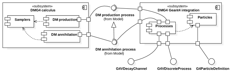
II DMG4 package structure
Structurally, the DMG4 package consists of two main components: a set of lower-level routines responsible for DM-related calculus, and a layer of Geant4 interfaces realization. This way various numerical tests and model benchmarking can be implemented using only the numerical routines part, before it gets embedded into Geant4 pipeline.
As for numerical routines, every process subclasses common parent root DarkMatter (being an abstract product in terms of factory pattern) facilitating common requirements for dark matter models in terms of mean free path, spatial dependencies on cross sections, decay width, etc. Subclasses implementing a particular model (concrete products) implement its interface (DM production process) by overriding certain virtual methods of DarkMatter base class.

The base DarkMatter class is extended by the DM annihilation process interface within DarkMatterAnnihilation. The DM annihilation process appends contract with routines yielding certain resonant-specific quantities (additional yield factor and angular distribution PDF). The diagram 1 illustrates relationships between interfaces and corresponding implementation classes with dark axial and dark photon modules as examples of concrete products. A particular sampler instance can be associated with physics model at the most abstract level.
Component diagram 2 provides a wider view on how particular numerical routines are exposed in terms of Geant4 API (namely, G4ParticleDefinition and G4VDiscreteProcess). Corresponding interfaces are implemented within the interim layer composed of a set of processes and related particles while the cross-section calculus is expressed by means of internal classes.
The DM sector particles introduced in the package are listed in Table 1. The PDG codes are ascribed according to the slightly extended rules in [11]. As compared to early versions, we reduced the number of mediator particle classes, which was possible due to usage of a new class DarkMatterParametersFactory. Using this class it is more convenient to specify the decay modes and some other parameters of particles. On the other hand, we added several DM particles of models with semivisible decay modes. Note that in many configurations we assume the mediators to be stable, although in full models they decay into stable DM particles. But for the missing energy signature simulation it is unimportant as the energy carried away is the same.
| Name | PDG ID | emitted by | spin | parity | Model | stable? | decay |
| DMParticleAPrime | 5500022 | 1 | 1 | true | - | ||
| 5500122 | Visible X | false | |||||
| 5500222 | B - L | false | , etc. | ||||
| 5500322 | Inelastic DM | false | |||||
| DMParticleScalar | 5400022 | 0 | 1 | true | - | ||
| 5400022 | Visible X | false | |||||
| DMParticlePseudoScalar | 5410022 | 0 | -1 | true | - | ||
| 5410122 | Visible X | false | |||||
| DMParticleAxial | 5510022 | 1 | -1 | true | - | ||
| 5510122 | |||||||
| DMParticleZPrime | 5500023 | 1 | 1 | true | - | ||
| 5500023 | false | , | |||||
| DMParticleALP | 5300122 | 0 | -1 | false | |||
| DMParticleChi1 | 5200014 | mediator | 1/2 | 1 | Inelastic DM | true | - |
| DMParticleChi2 | 5200013 | mediator | 1/2 | 1 | Inelastic DM | false | |
| DMParticleChi | 5200012 | mediator | 1/2 | 1 | true | - |
The dark sector particles are assumed to be stable as they are anyway undetectable. This does not apply to the appearing in models of inelastic Dark Matter[12]. For this particle, the 3-body decay is simulated using the matrix element sampling implemented in the new G4iDM3bodyDecayChannel class, as explained in Sec.IV.
The current version of DMG4 package contains the following processes of DM production:
-
•
Bremsstrahlung-like process of the type , where is a projectile (can be ), and is a DM mediator. Apart from the mediators listed in the table, we added a process with a spin 2 particle without adding a corresponding particle class. It means it is possible to simulate the invisibly decaying spin 2 mediator.
-
•
Primakoff process of photon conversion , where is an axion-like particle (ALP) [13]
-
•
Resonant in-flight positron annihilation on atomic electrons , where is a dark matter mediator decay product [14].
The physics for a simulation run is configured in the function DarkMatterPhysicsConfigure called from the constructor of the steering class DarkMatterPhysics. The configuration is done using the singleton class DarkMatterParametersFactory. A user specifies a number of parameters, then the steering class performs the needed actions:
-
•
Creates an instance of one of the concrete classes corresponding to the needed process and derived from the base class DarkMatter, for example DarkPhotons
-
•
Instantiates and registers the needed particles and processes provided by the DMG4 package in terms of the native Geant4 API.
The following main parameters are to be specified: 1. The process code; 2. The mixing (or coupling) parameter ; 3. The mediator mass; 4. The decay mode; 5. The cut-off minimal energy of particles that can initiate the processes of DM production. The latter is needed to avoid the simulation of very soft DM particles that are anyway undetectable. In the new versions, this parameter also specifies, for some processes or for a part of the mediator mass range, a minimal mediator energy that is allowed to be generated.
III Package DarkMatter
This class, which we try to keep as weakly connected to Geant4 as possible, contains the methods that return total and differential cross sections, first of all for the bremsstrahlung processes. For these processes the cross sections can be calculated numerically at Exact Tree Level (ETL) or using the formulas of Weizsaker-Williams (WW) and improved Weizsaker-Williams (IWW) approximations [1].
As explained in [6], for the electron beam it contains the tabulated K-factors that correct the total cross sections obtained in IWW approximations for the electron beam to the values calculated at ETL. As compared to the previous version, we extended the corresponding tables down to the mediator masses of 1 keV and, for some classes, up to 3 GeV.
In addition to this, we also tabulated the differential cross sections for the electron beam and mediator masses below 1 MeV, where it can have non-trivial shape, significantly different from the sharply peaked one at around for heavier mediators.
The Lagrangians and initial cross section formulas used in the package can be found in the previous paper [6]. The Lagrangian for the new model with spin 2 mediator looks like this [15, 16, 17]:
| (1) | |||
where is the label of the SM electron, is a stress tensor of the SM photon field , is a covariant derivative of the gauge field, and is the dimensional parameter for spin-2 interactions, that is associated with the scale of new physics; and are dimensionless couplings for the electron and photon respectively. We choose the universal coupling throughout the paper.
Finally, since the early versions of the package, significant progress has been made in the cross sections for the case of a muon beam and in the annihilation processes. These, alongside other developments, are described in the following sections.
IV Inclusion of inelastic Dark Matter models
In multi-generational dark sector models, such as scenarios involving inelastic Dark Matter, the dark photon exhibits off-diagonal couplings to a pair of particles, denoted as and , with different masses. The heavier particle, , is unstable and decays via the channel . In such cases, the dark photon decay cascade leads to both visible and invisible final states and is consequently referred to as semivisible .
To enable the simulation of these next-to-minimal models, two new particles, DMParticleChi1 and DMParticleChi2, have been added to the DMG4 package. Notably, two distinct semivisible models are now included: inelastic Dark Matter (iDM) [12] and inelastic Dirac Dark Matter (i2DM) [18]. The decay widths for these models are taken from Refs. [19, 20] and Ref.[18] respectively.
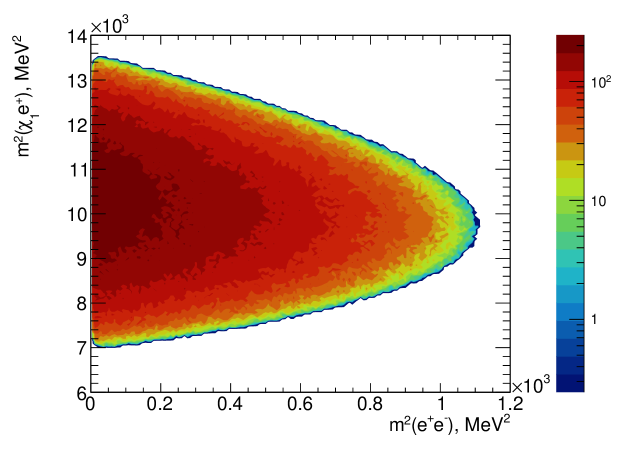
To account for the specific 3-body decay process , the DMG4 class G4iDM3bodyDecayChannel has been implemented. This class, derived from G4VDecayChannel and based on G4DalitzDecayChannel, performs the sampling of the spin-averaged matrix element, as illustrated in Fig. 3. The kinematics of the final state particles is subsequently calculated based on the obtained squared invariant masses of the and systems.
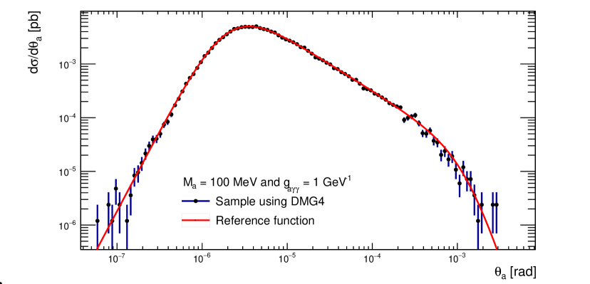
V Angular sampling of ALP production via Primakoff effect
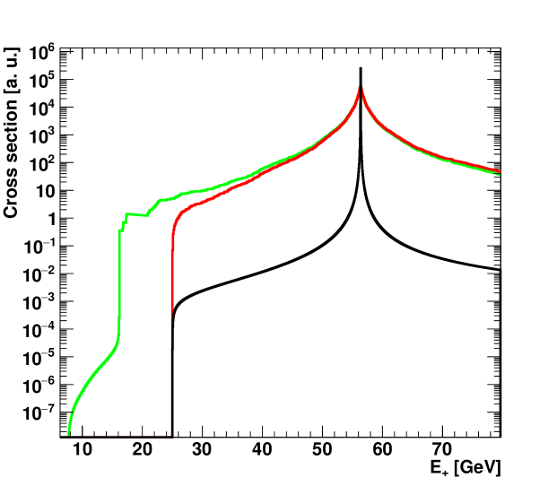
In order to simulate the final state kinematics of the ALP produced in the Primakoff process , the sampling of the emission angle was implemented in DMG4. The differential cross section with respect to the angle of ALP emission is obtained in the limit when and and is used in the sampling scheme, as presented in our previous work [13]. In this approximation the energy of the emitted ALP can be calculated based on the angle . The results of the angular sampling are displayed in Fig. 4 and compared to the reference distribution function, which is a single differential cross section.
VI Developments in muon-philic processes and cross sections implementations
In this section, we describe the recent developments in the simulation of light dark matter production in bremsstrahlung-like reactions of muons on nuclei, . In particular, we describe the extension of muon-philic models to different mediator types and the improvements in the underlying production cross sections implementation.
VI.1 Broadening the class of mediators
In our previous work [6], the emission of a light mediator from muons was associated with the gauge vector boson, , [21, 22, 23, 24, 25, 26]. Within this model, the illustrative Lagrangian of the theory is given by
| (2) |
where is the field strength tensor associated with the field, the mass of the gauge boson, the coupling to SM leptons and the left-handed chiral projection operator. The decay width associated with the vanilla model is given by the purely invisible channel to SM neutrinos, , such that
| (3) |
where .
The addition to the aforementioned model, the formulas for other types of light muon-philic mediators is provided, namely for scalar and
pseudoscalar particles, respectively and , with corresponding simplified Lagrangians
| (4) |
| (5) |
where it is assumed that the mediators do not need to couple to neutrinos, have masses and and muon-specific couplings and .
VI.2 Calculations of the production cross sections
As introduced in Sec. III, the differential and total production cross sections for the reaction can be computed within the WW approximation. Within this phase-space approximation, the process depicted above is factorized through the use of the equivalent photon flux approximation [27, 28] into a process, provided the virtual photon flux
| (6) |
with and being the minimum and maximum momentum transfer to the nucleus, and the elastic form factor associated with the nucleus (see e.g. [27]). As such, the double-differential cross section reads [29]
| (7) |
with , and being respectively the fractional energy of the boson and its emission angle, the fine structure constant, the corresponding Lorentz factor, and the four-momenta associated with the initial-state muon and final-state boson, and the muon energy before the interaction. Together with the double differential cross section of Eq. (7), we implemented within the DarkMatter package the single-differential cross section for , obtained by performing a complicated analytical integration of Eq. (7). This allowed us to obtain much better run-time performance of the event sampling code. The total cross section then reads [30]
| (8) |
where the six special functions , and the definition of the variable and
can be found in [30]. This provides one with a more precise expression than within the IWW approximation, where the dependence on
is neglected in Eq. (6). As a result, we don’t need K-factors and tables for muon-beam-related simulations.
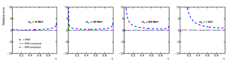
For an appreciable estimate of the precision of the analytical results of the WW approximation
integration, a comparison of the single-differential cross section with both ETL
and IWW results is shown in Fig. 5 for different in the scenario. The relative error between
the computations at ETL and within the WW phase-space approximation is , while both the WW numerical and analytical methods
agree well within . The reader is referred to [29] and [30] for a more in-depth discussion
of the errors.

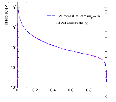
As a final test, the implementation of the vector boson emission process in the mass limit is compared to the Geant4 treatment of SM muon bremsstrahlung, . The comparison is driven against the absolute yields of both processes. As such, those are extracted from a minimal Geant4 simulation of muons impinging on a thick block of lead (Pb). The parameters and production cuts of the G4MuBremsstrahlungModel are chosen to be comparable with the one of DarkZ, namely similar values of and , and equal parameters and (respectively and within Geant4, see [31]), as well as a 1 GeV production cut (emission threshold). This later choice implies that the cross sections do not depend on the mass for values below 0.1 MeV. The results for mono-energetic 160 GeV muons with are shown in Fig. 6. Within the statistical uncertainties, it is found that the absolute yields agree within .
VI.3 Final-state muon kinematics
As compared to the experiments in electron/positron beams, for the muon beam the sampling of the recoil muon kinematic variables is much more important. This is due to the fact that the missing energy in this case is determined by measuring the recoil muon momentum by tracker. Similarly to Eq. (7), for the recoil muon variables we have
| (9) |
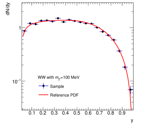
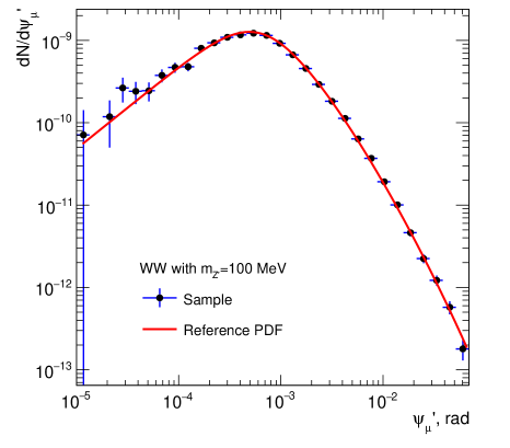
where is the final-state muon fractional energy, is its emission angle, is its Lorentz factor and is its four-momentum. The corresponding double differential cross section is implemented in the package DarkMatter. For illustrative purposes, the results of events sampling for both the and variables are shown Fig. 7, as extracted from a DMG4-based simulation of light production with fixed mass MeV. The validity of the implementation is inferred through a Kolmogorov-Smirnov (KS) test [32, 33] for the goodness of the fit, comparing both the target partial distribution function (PDF) and the corresponding sampled histogram, and indicating for the test mass range MeV that the identity null hypothesis is accepted at a 0.05 significance level.
VII Developments in the annihilation processes
In this section, we describe the main DMG4 developments and improvements concerning light dark matter production via resonant annihilation. We refer the reader to our previous work [6] for a comprehensive discussion regarding the general implementation of this process in the package.
VII.1 Extension to different models
For the four mediator cases already implemented in the DMG4 package, , where
can be a vector, axial-vector, scalar, and pseudo-scalar particle, we introduced the possibility for the final state DM particles
to be (complex) scalars. Specifically, we considered the following Lagrangians, where is the LDM complex scalar
field, is a SM charged field. , , , are the mediators field, while are the mixing (or coupling) parameters. Finally, are the masses of the mediators.
Vector case:
| (10) |
Axial vector case:
| (11) |
Scalar case:
| (12) |
Pseudo-scalar case:
| (13) |
The corresponding cross sections for the processes implemented in the code reads
| (14) |
where is the invariant mass of the system, the mediator mass, , is the intermediate DM particle decay width to dark particles , is the electromagnetic fine structure constant, and is the coupling squared to the dark particles . Finally, is a kinematic factor that reads, respectively, for the vector and axial-vector mediator, and for the scalar and pseudo-scalar cases. Finally, the decay widths read:
| (15) | |||||
| (16) | |||||
| (17) | |||||
| (18) |
where .
For the vector-mediator model, we also considered an inelastic (i.e., non-diagonal) model foreseeing two fermionic LDM states and with different masses and , with [20]. In this model, at tree level only the vertex exists. The corresponding Lagrangian reads:
| (19) |
The corresponding annihilation cross section reads:
| (20) |
where is the and three-momentum in the rest frame, while and are the final state particles total energies in the same frame. The decay width for the channel is:
| (21) |
In this DMG4 software version, we also included the possibility to simulate the process, where the intermediate particle is the massive force mediatior associated with a new SM gauge symmetry involving the neutrino sector. Specifically, we considered the two cases of a gauge symmetry and a one [34, 35]. While the first case resembles that of a vector dark photon by making the substitution , where is the gauge coupling constant, for the second scenario at tree level the couples only to second and third generation leptons. Nevertheless, thanks to the photon- coupling introduced at next-to-leading order by loops involving muon and tau leptons, an effecting vertex appears, with coupling , where is the four-momentum squared. The function reads:
| (22) |
In the code, we were able to introduce the full analytical expression for the function, allowing to optimize the corresponding computation time. This is given by the formula:
| (23) |
with and .
VII.2 Narrow-width resonance production
The introduction of all new DMG4 processes in Geant4 is based on the G4VDiscreteProcess class - each process is described by a new class inheriting from the latter. In particular, each class has to provide a concrete implementation of the two pure virtual methods GetMeanFreePath and PostStepDoIt; in particular, the first method is responsible of computing the positron mean free path for the annihilation process at the beginning of each Geant4 step, when the step-length is not yet determined, from the knowledge of the corresponding G4Track. It follows that, if the cross section for the annihilation process is computed solely from the value of the positron energy at the beginning of the step , without accounting for the full cross-section energy dependence, the obtained result would under-estimate (over-estimate) the average value along the step if (), where is the positron resonant energy in the laboratory frame. While in the case of a broad resonance this effect is not critical, if the typical energy loss across a Geant4 step is significantly larger than the mediator width , it could induce a significant distortion of the simulation results in case of a narrow resonance - this is the case, for example, of the model described previously in the text. Two ad-hoc modifications were introduced in the code to account for this effect.
VII.2.1 Energy dependence of the cross section
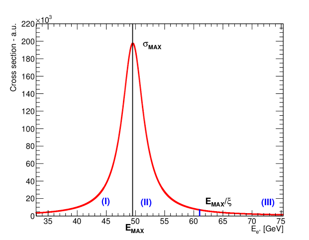
As discussed previously, the G4VDiscreteProcess-based implementation requires to compute the cross section for the annihilation process at the beginning of each Geant4 step, before the latter is determined. To account for the energy dependency of the cross section, we followed the strategy implemented in Geant4 for other electromagnetic-like processes and described in the manual, based on the sole assumption that the cross section has only one maximum , for . Specifically, our implementation assumes that, during the step still to be computed, the cross section will be lower than a certain value . The mean free path for the process is then computed via . If this process is selected by Geant4 as that taking place and limiting the next step length, the final state sampling, implemented via the PostStepDoIt method, is invoked with reduced probability , where is the positron energy at the end of the step; alternatively, nothing happens and the positron tracking continues. In the following we call this procedure “Maximum-Rejection”. We underline that it is not obvious that in this procedure should be computed considering the cross section at the end of the step and not the average value along the step111Incidentally, we note that in the Geant4 physics reference manual for release 11.2, rev 8.0, in Sec. 7.4 “Correcting the Cross Section for Energy Variation” the prescription to use of in the computation of is supported by a reference to [39]. However, in that work no justification of this method is provided.. To empirically verify this, we made a dedicated toy-MC study, presented in Appendix A.
The value is selected as follows, dividing the positron energy range in three dinstinct intervals, also shown in Fig. 8. The first case corresponds to the condition : in this case, the positron energy is already lower than the cross section maximum, and will further decrease along the positron trajectory; therefore, . In the second case, instead, , where is a dimensionless parameter to be appropriately tuned; this case corresponds to a positron with initial energy close to that of the resonance, and assumes . Finally, if , then .
The parameter controls the transition between case (II) and case (III), and is connected to the typical positron energy loss across a step. If the typical value of the continuous energy loss across a step is , then the value of can be set from the requirement that, for a positron initial energy in the interval , where is a safety factor, case (II) should be applied, since it is possible that, in the next step, the particle will loose enough energy to cross the resonant energy. All values of in the interval satisfy this requirement. In the code, the lower limit of the interval is used.
VII.2.2 Dynamical step limitation
The approach presented in the previous section only considers continuous energy losses for the positron, but not the discrete ones associated to bremsstrahlung emission, that may significantly alter the positron energy. Also, this approach is expected to work well for geometries with many geometrical boundaries, forcing many positron steps, but can be inaccurate for large homogeneous volumes. To partially compensate for this, we implemented a step limitation for positrons. The intrinsic scale of the positron step limitation for narrow resonance production is given by the ratio of the modified resonance width , where the factor is a kinematic correction induced by the Lorentz transformation from the center-of-mass frame to the laboratory one, and the positron energy loss per unit length , .
In order to optimize the computation time, we use a dynamical step limitation for positrons, based on the relative cross section variation with respect to the energy: the more the cross section is expected to vary for a given positron energy, the smaller the maximum step allowed for the positron. The resonant annihilation cross section can indeed be written as , where is a smooth-varying function of the positron energy. It follows that the relative cross section variation with respect to the energy reads:
| (24) |
This function has two maxima at , where . To avoid numerical instabilities in the interval between these two values, associated with the zero at , we slightly modified it to be if , and otherwise. In the code, we thus define the positron step limit as .
VII.3 Atomic effects in annihilation
In the previous DMG4 version, all annihilation processes were handled by considering the atomic electron to be at rest in the laboratory frame. Atomic motions reflect to a broadening of the annihilation cross section , since a given positron energy can reflect to different values of the Mandelstam variable for the electron-positron system, defined by the equation:
| (25) |
where () is the atomic electron total energy (three-momentum), and is the cosine of the angle between the and momenta. From this, it follows that a positron whose energy won’t match the resonance mass if annihilating with an at-rest electron can do so for an orbiting one and vice-versa, resulting to a broad range of energies that can contribute to the process. To illustrate this effect, we consider the case of a MeV mediator, and an electron kinetic energy of about 10 keV (typical value for lead): the positron energy in the laboratory frame resulting to spans a range from 40.7 GeV to 60.3 GeV (for comparison, the at-rest value is 48.6 GeV). Similarly, for MeV, considering an electron kinetic energy of about 290 eV (typical value for carbon), the resonant positron energy in the laboratory frame spans from 273 MeV to 291 MeV. From this consideration, it follows that the at-rest approximation is justified for large-width resonances, when , while it can’t be applied in the narrow width scenario.
In this DMG4 software version, we implemented a full calculation involving atomic motions as follows. For the simpler case of massless final state particles, such as in the reaction , the general expression for the cross section can be written as , where is a smooth-varying function of the impinging positron energy, and , are, respectively, the mediator mass and total width. By substituting the previous expression for , this translates to:
| (26) |
The code computes, for each interaction, the average value of this expression, by considering an isotropic electron motion, i.e. a flat PDF for in the interval:
| (27) | ||||
| (28) |
where and ( and ) are the positron and the electron total energies (momenta) in the laboratory frame, and within the integration interval.
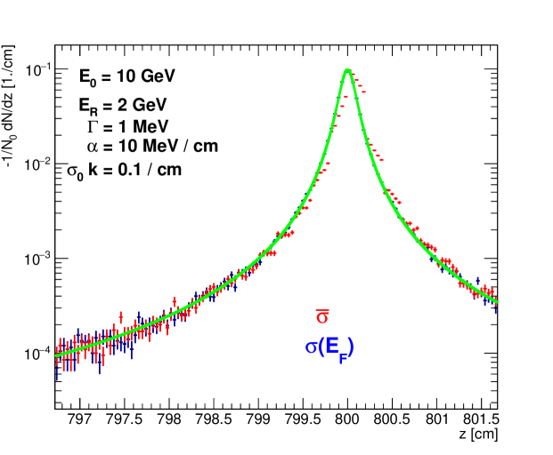
Concerning the atomic electron energies, the code currently implements two possible models. The first, simplified model assumes, for each atomic shell, a fixed kinetic energy equal to the binding energy magnitude, , and computes the average cross section by summing over the atomic shells, considering for each a weight proportional to the occupation number. The shells atomic energies for the target material are obtained directly from Geant4, using the G4Element::GetAtomicShell method. Similarly, the occupation numbers are obtained from the G4Element::GetNbOfShellElectrons method. In the second, more realistic model, used by default, an exponential PDF distribution 222We incidentally note that this model is the same adopted by the Geant4 software to handle atomic motion effects in Compton scattering. for is considered, . The contribution for each shell is separately computed, by integrating the expression for over , and summing the contributions with weights each equal to the shell occupation number. The code computes the integral over numerically through the Monte Carlo method. To speed-up the computation time, since the expression for is independent from the positron kinematics, a set of random electron kinetic energies is pre-generated for each atomic shell at initialization time. The effect of the inclusion of atomic motion description in the software is illustrated in Fig. 9, showing the annihilation cross section as a function of the positron energy for a 225 MeV resonance, having a width of 7 keV. The black curve is the result obtained without considering atomic motions, while the red (green) curve are the results obtained from the first and second model described before. In the first case, the discreteness of the atomic shells kinetic energies is clearly visible.

This approach is slightly modified for the more general case involving equally massive particles in the final state, such as in the LDM production process , since in this case the function is proportional to the final-state momentum , that intrinsically contains a kinematic threshold333The extension of the code to handle final state with particles having different masses is foreseen for the next DMG4 release.. Starting from the previous for in Eq. 27, and writing explicitly the factor, the expression for is:
| (29) |
where . The integration range can more easily be determined by changing the integration variable from to for fixed , and explicitly setting :
| (30) |
and considering the threshold requirement . From the identity , it follows that . Note that if , then the positron energy is incompatible with for all angles, and thus . If, instead, , the integral is still performed only in the physical region up to . The result of the integral, assuming a constant value for and defining is:
| (31) |
where is given by:
| (32) | ||||
| (33) |
where and . Finally, to handle the residual (and thus ) dependency in for fixed values of and , this term is computed event-by-event via Monte Carlo integration, taking 20 uniformly-spaced values in the allowed interval and averaging over the corresponding values. As an example, Fig. 10 shows the obtained cross section, considering the more realistic model for atomic electrons energies, for a 270 MeV mediator with keV, decaying into 90 MeV final state particles. In this configuration, for the annihilation with at-rest electrons, the positron threshold energy would be approximately 25 GeV, but thanks to atomic motions also lower-energy positrons can undergo this reaction.
VIII Conclusion
The package DMG4 for the simulation of light dark matter production in fixed target experiments is created. It can be used in full simulation programs based on the Geant4 framework. The subpackage DarkMatter containing a collection of cross sections is weakly connected to Geant4, thus can be used in programs based on other frameworks. The package is widely used in the NA64 experiment.
In this paper, numerous developments of the the package are presented, in particular the WW approximation cross sections for the muon beam [30], models with semivisible (inelastic Dark Matter) [18] and several important improvements for the annihilation processes.
The package is available at http://mkirsano.web.cern.ch/mkirsano/DMG4.tar.gz and https://gitlab.cern.ch/P348/DMG4 (internal NA64 repository). It is recommended also to contact the corresponding author Mikhail Kirsanov about the usage.
IX Acknowledgements
This work was supported by the Ministry of Science and Higher Education (MSHE) and RAS (Russia), MSHE Project FSWW-20230003, Tomsk Polytechnic University within the assignment of MSHE (Russia), the European Research Council (ERC) under the European Union’s Horizon 2020 research and innovation program (Grant agreement No. 947715 - POKER Starting Grant). This work is partially supported by ICSC – Centro Nazionale di Ricerca in High Performance Computing, Big Data and Quantum Computing, funded by European Union – NextGenerationEU. This work is also supported by RyC-030551-I, PID2021-123955NA-100 and CNS2022-135850 funded by MCIN/AEI/FEDER, UE (Spain) and by ETH Zurich and SNSF Grants No. 186181, 186158, 197346, 216602 (Switzerland).
X Appendix A
In order to check the the procedure “Maximum-Rejection” we considered a simple model where there is a pseudo-positron particle moving forward in a material and loosing a constant, deterministic amount of energy per unit length. Therefore, if the pseudo-positron pseudo-positron enters in this material at with initial energy , the energy at depth in the material is given by , for . The only other process available for this particle is the annihilation process, with a simplified cross section formula .
If a mono-chromatic beam of pseudo-positrons impinges on the material at , the number of particles at a given depth in the material can be computed from the following equation:
| (34) |
where is the number density of electrons per unit volume in the material. This equation can be solved exactly, obtaining:
| (35) |
This gives a number of interactions per unit length, , equal to:
| (36) |
To check the “Maximum-Rejection” procedure we made a toy Monte Carlo simulation, accounting for the energy variation across the step as discussed in Sec. VII.2.1. Specifically, we implemented a first version computing the reduced probability through the cross section at the end of the step, as recommended in the Geant4 manual, and also by using the mean cross section value along the step. The result is shown in Fig. 11. This test confirms the solution suggested by the Geant4 manual.
References
- Bjorken et al. [2009] J. D. Bjorken, R. Essig, P. Schuster, and N. Toro, Phys. Rev. D 80, 075018 (2009), arXiv:0906.0580 [hep-ph] .
- Izaguirre et al. [2013] E. Izaguirre, G. Krnjaic, P. Schuster, and N. Toro, Phys. Rev. D 88, 114015 (2013), arXiv:1307.6554 [hep-ph] .
- Batell et al. [2009] B. Batell, M. Pospelov, and A. Ritz, Phys. Rev. D 80, 095024 (2009), arXiv:0906.5614 [hep-ph] .
- Izaguirre et al. [2015] E. Izaguirre, G. Krnjaic, P. Schuster, and N. Toro, Phys. Rev. D 91, 094026 (2015), arXiv:1411.1404 [hep-ph] .
- Agostinelli et al. [2003] S. Agostinelli et al. (GEANT4), Nucl. Instrum. Meth. A 506, 250 (2003).
- Bondi et al. [2021] M. Bondi, A. Celentano, R. R. Dusaev, D. V. Kirpichnikov, M. M. Kirsanov, N. V. Krasnikov, L. Marsicano, and D. Shchukin, Comput. Phys. Commun. 269, 108129 (2021), arXiv:2101.12192 [hep-ph] .
- Holdom [1986] B. Holdom, Phys. Lett. B 166, 196 (1986).
- Battaglieri et al. [2017] M. Battaglieri et al., in U.S. Cosmic Visions: New Ideas in Dark Matter (2017) arXiv:1707.04591 [hep-ph] .
- Beacham et al. [2020] J. Beacham et al., J. Phys. G 47, 010501 (2020), arXiv:1901.09966 [hep-ex] .
- ISO Central Secretary [2012] ISO Central Secretary, Information technology – Object Management Group Unified Modeling Language (OMG UML) – Part 1: Infrastructure, Standard ISO/IEC 19505-1:2012 (International Organization for Standardization, Geneva, CH, 2012).
- [11] Monte Carlo Particle Numbering Scheme, https://pdg.lbl.gov/2019/reviews/rpp2019-rev-monte-carlo-numbering.pdf, accessed: 2021-01-25.
- Tucker-Smith and Weiner [2001] D. Tucker-Smith and N. Weiner, Phys. Rev. D 64, 043502 (2001), arXiv:hep-ph/0101138 .
- Dusaev et al. [2020] R. R. Dusaev, D. V. Kirpichnikov, and M. M. Kirsanov, Phys. Rev. D 102, 055018 (2020), arXiv:2004.04469 [hep-ph] .
- Marsicano et al. [2018] L. Marsicano, M. Battaglieri, M. Bondí, C. D. R. Carvajal, A. Celentano, M. De Napoli, R. De Vita, E. Nardi, M. Raggi, and P. Valente, Phys. Rev. Lett. 121, 041802 (2018), arXiv:1807.05884 [hep-ex] .
- Voronchikhin and Kirpichnikov [2022] I. V. Voronchikhin and D. V. Kirpichnikov, Physical Review D 106, 10.1103/physrevd.106.115041 (2022).
- Lee et al. [2014] H. M. Lee, M. Park, and V. Sanz, Eur. Phys. J. C 74, 2715 (2014), arXiv:1306.4107 [hep-ph] .
- Kang and Lee [2020] Y.-J. Kang and H. M. Lee, The European Physical Journal C 80, 10.1140/epjc/s10052-020-8153-x (2020), arXiv:2001.04868 .
- Filimonova et al. [2022] A. Filimonova, S. Junius, L. L. Honorez, and S. Westhoff, Journal of High Energy Physics 2022, 10.1007/jhep06(2022)048 (2022).
- Mohlabeng [2019] G. Mohlabeng, Phys. Rev. D 99, 115001 (2019), arXiv:1902.05075 [hep-ph] .
- Cazzaniga et al. [2021] C. Cazzaniga et al. (NA64), Eur. Phys. J. C 81, 959 (2021), arXiv:2107.02021 [hep-ex] .
- He et al. [1991a] X. G. He, G. C. Joshi, H. Lew, and R. R. Volkas, Phys. Rev. D 43, 22 (1991a).
- He et al. [1991b] X.-G. He, G. C. Joshi, H. Lew, and R. R. Volkas, Phys. Rev. D 44, 2118 (1991b).
- Foot et al. [1994] R. Foot, X. G. He, H. Lew, and R. R. Volkas, Phys. Rev. D 50, 4571 (1994), arXiv:hep-ph/9401250 .
- Altmannshofer et al. [2016] W. Altmannshofer, S. Gori, S. Profumo, and F. S. Queiroz, JHEP 12, 106, arXiv:1609.04026 [hep-ph] .
- Kile et al. [2015] J. Kile, A. Kobach, and A. Soni, Phys. Lett. B 744, 330 (2015), arXiv:1411.1407 [hep-ph] .
- Park et al. [2016] J.-C. Park, J. Kim, and S. C. Park, Phys. Lett. B 752, 59 (2016), arXiv:1505.04620 [hep-ph] .
- Liu et al. [2017] Y.-S. Liu, D. McKeen, and G. A. Miller, Phys. Rev. D 95, 036010 (2017), arXiv:1609.06781 [hep-ph] .
- Liu and Miller [2017] Y.-S. Liu and G. A. Miller, Phys. Rev. D 96, 016004 (2017), arXiv:1705.01633 [hep-ph] .
- Kirpichnikov et al. [2021] D. V. Kirpichnikov, H. Sieber, L. M. Bueno, P. Crivelli, and M. M. Kirsanov, Phys. Rev. D 104, 076012 (2021), arXiv:2107.13297 [hep-ph] .
- Sieber et al. [2023] H. Sieber, D. V. Kirpichnikov, I. V. Voronchikhin, P. Crivelli, S. N. Gninenko, M. M. Kirsanov, N. V. Krasnikov, L. Molina-Bueno, and S. K. Sekatskii, Phys. Rev. D 108, 056018 (2023), arXiv:2305.09015 [hep-ph] .
- Bogdanov et al. [2006] A. G. Bogdanov, H. Burkhardt, V. N. Ivanchenko, S. R. Kelner, R. P. Kokoulin, M. Maire, A. M. Rybin, and L. Urban, IEEE Trans. Nucl. Sci. 53, 513 (2006).
- Kolmogorov [1933] A. Kolmogorov, G. Ist. Ital. Attuari. 4, 83 (1933).
- Smirnov [1948] N. Smirnov, Ann. Math. Statist. 19, 279 (1948).
- Andreev et al. [2022a] Y. M. Andreev et al. (NA64), Phys. Rev. D 106, 032015 (2022a), arXiv:2206.03101 [hep-ex] .
- Andreev et al. [2022b] Y. M. Andreev et al. (NA64), Phys. Rev. Lett. 129, 161801 (2022b), arXiv:2207.09979 [hep-ex] .
- Note [1] Incidentally, we note that in the Geant4 physics reference manual for release 11.2, rev 8.0, in Sec. 7.4 “Correcting the Cross Section for Energy Variation” the prescription to use of in the computation of is supported by a reference to [39]. However, in that work no justification of this method is provided.
- Note [2] We incidentally note that this model is the same adopted by the Geant4 software to handle atomic motion effects in Compton scattering.
- Note [3] The extension of the code to handle final state with particles having different masses is foreseen for the next DMG4 release.
- Ivanchenko et al. [1991] V. N. Ivanchenko, A. D. Bukin, M. S. Dubrovin, S. I. Eidelman, N. A. Grozina, and V. A. Tayursky, in Workshop on Detector and Event Simulation in High-energy Physics (MC ’91) (1991) pp. 79–85.