Abstract

In this work, we use optical theorem to calculate the next-to-leading order corrections to the spectral densities directly in the QCD sum rules for the pseudoscalar and scalar $B_{c}$ mesons. We take the experimental data as guides to perform updated analysis, and obtain the masses and decay constants, therefore the leptonic decay widths, which can be confronted to the experimental data in the future.

PACS number: 12.38.Bx, 12.38.Lg

Key words: Next-to-leading order contributions, QCD sum rules

1 Introduction

In 1998, the CDF collaboration observed the pseudoscalar $B_{c}$ mesons through the decay modes $B_{c}^{\pm}\to J/\psi\ell^{\pm}X$ and $B_{c}^{\pm}\to J/\psi\ell^{\pm}\bar{\nu}_{\ell}$ in the $p\bar{p}$ collisions at the energy $\sqrt{s}=1.8\,\rm{TeV}$ at the Fermilab Tevatron, the measured mass is $6.40\pm 0.39\pm 0.13\,\rm{GeV}$ [1, 2].

In 2007, the CDF collaboration confirmed the $B_{c}$ mesons through the decay modes $B_{c}^{\pm}\to J/\psi\pi^{\pm}$ with the measured mass $6275.6\pm 2.9\pm 2.5\,\rm{MeV}$ [3]. In 2008, the D0 collaboration reconstructed the $B_{c}^{\pm}\to J/\psi\pi^{\pm}$ decays and confirmed the $B_{c}$ mesons with the measured mass $6300\pm 14\pm 5\,\rm{MeV}$ [4]. Now the average value listed in the Review of Particle Physics is $6274.47\pm 0.27\pm 0.17\,\rm{MeV}$ [5].

In 2014, the ATLAS collaboration reported the observation of a structure in the $B_{c}^{\pm}\pi^{+}\pi^{-}$ invariant mass spectrum, which is consistent with the predicted $B_{c}^{\prime}$ meson with a mass of $6842\pm 4\pm 5\,\rm{MeV}$ [6].

In 2019, the CMS collaboration observed two excited $\bar{b}c$ states in the $B^{+}_{c}\pi^{+}\pi^{-}$ invariant mass spectrum, which are consistent with the $B^{\prime+}_{c}$ and $B_{c}^{*\prime+}$, respectively [7]. The two states are separated in mass by $29.1\pm 1.5\pm 0.7\,\rm{MeV}$, and the mass of the $B^{\prime+}_{c}$ is measured to be $6871.0\pm 1.2\pm 0.8\pm 0.8\,\rm{MeV}$. Also in 2019, the LHCb collaboration observed the excited $B^{\prime+}_{c}$ and $B_{c}^{*\prime+}$ mesons in the $B^{+}_{c}\pi^{+}\pi^{-}$ invariant mass spectrum. The $B_{c}^{*\prime+}$ meson has a mass of $6841.2\pm 0.6\pm 0.1\pm 0.8\,\rm{MeV}$, which is reconstructed without the low-energy photon emitted in the $B_{c}^{*+}\to B_{c}^{+}\gamma$ decay following the process $B_{c}^{\prime*+}\to B_{c}^{*+}\pi^{+}\pi^{-}$, while the $B^{\prime+}_{c}$ meson has a mass of $6872.1\pm 1.3\pm 0.1\pm 0.8\,\rm{MeV}$ [8].

It is odd that the $B_{c}^{\prime}$ meson emerges as heavier than the mass of the $B_{c}^{*\prime}$ meson, which is in conflict with all the theoretical estimations, this maybe or maybe not due to impossibility of reconstruction of the low-energy photon in the $B_{c}^{\ast+}\rightarrow B_{c}^{+}\gamma$ decay [9]. Only the $B_{c}$ and $B_{c}^{\prime}$ mesons are listed in Review of Particle Physics [5], which are in contrary to the copious (well-established) spectroscopy of the charmonium and bottomonium states. Despite the enormous developments on the heavy quark physics in recent years, the bottom-charm spectroscopy remains poorly known, which calls for further investigations.

The beauty-charm mesons provide an optimal laboratory for exploring both the perturbative and nonperturbative dynamics of the heavy quarks, due to absence of the light quark’s contamination, and for exploring the strong and electro-weak interactions, as they are composed of two different heavy flavors and cannot annihilate into gluons or photons. For the excited $c\bar{b}$ states, which lie below the $BD$ threshold, would decay into the $B_{c}$ meson through the radiative decays or hadronic decays [10, 11], while the ground state $B_{c}$ can only decay weakly through emitting a virtual $W$-boson.

There have been several theoretical works on the mass spectroscopy of the bottom-charm mesons, such as the relativized (or relativistic) quark model with an special potential [10, 11, 12, 13, 14], the nonrelativistic quark model with an special potential [15, 16, 17, 18, 19, 20, 21, 22, 23], the semi-relativistic quark model using the shifted large-$N$ expansion [24, 25], the perturbative QCD [26], the nonrelativistic renormalization group [27], the lattice QCD [28, 29, 30, 31], the Bethe-Salpeter equation [32, 33, 34], the full QCD sum rules [35, 36, 37, 38, 39, 40, 41], the potential model combined with the QCD sum rules [15, 16], etc.

With the continuous development in experimental techniques, we expect that more $c\bar{b}$ states would be observed in the future. The decay constant, which parameterizes the coupling between a current and a meson, plays an important role in exploring the exclusive processes, because the decay constants are not only a fundamental parameter describing the pure leptonic decays, but also are an universal input parameter related to the distribution amplitudes, form-factors, partial decay widths and branching fractions in many processes. By precisely measuring the branching fractions, we can resort to the decay constants to extract the CKM matrix element in the standard model and search for new physics beyond the standard model [42].

Decay constants of the bottom-charm mesons have been investigated in several theoretical approaches, such as the full QCD sum rules [35, 36, 37, 38, 39, 40, 41, 43, 44], the potential model combined with the QCD sum rules [15, 16], the QCD sum rule combined with the heavy quark effective theory [45, 46, 47, 48, 49, 50, 51, 52], the covariant light-front quark model [53, 54], the lattice non-relativistic QCD [31], the shifted large-$N$ expansion method [25], the field correlator method [55], etc. However, the values from different theoretical approaches vary in a large range, it is interesting to extend our previous works on the vector and axialvector $B_{c}$ mesons [40] to investigate the pseudoscalar and scalar $B_{c}$ mesons with the full QCD sum rules by including next-to-leading order radiative corrections and choose the updated input parameters, thus our investigations are performed in a consistent way. We take the experimental data as guides to choose the suitable Borel parameters and continuum threshold parameters, examine the masses and decay constants of the pseudoscalar and scalar $B_{c}$ mesons with the QCD sum rules, therefore we calculate the leptonic decay widths to be confronted to the experimental data in the future.

The article is arranged: we calculate the next-to-leading order contributions to the spectral densities and obtain the QCD sum rules in Sect.2; in Sect.3, we present the numerical results and discussions; and Sect.4 is reserved for our conclusions.

2 Explicit calculations of the spectral densities at the next-to-leading order

We write down the two-point correlation functions firstly,

$$\Pi_{P/S}(p^{2}) = i\int d^{4}xe^{ip\cdot x}\langle 0|T\left\{J(x)J^{\dagger}(0)\right\}|0\rangle\,,$$ (1)

where $J(x)=J_{P}(x)$ and $J_{S}(x)$,

$$J_{P}(x) = \bar{c}(x)i\gamma_{5}b(x)\,,$$

$$J_{S}(x) = \bar{c}(x)b(x)\,.$$ (2)

The correlation functions can be written in the form,

$$\Pi_{P/S}(p^{2}) = \frac{1}{\pi}\int_{(m_{b}+m_{c})^{2}}^{\infty}ds\frac{{\rm Im\Pi}_{P/S}(s)}{s-p^{2}}\,,$$ (3)

through dispersion relation, where

$$\frac{{\rm Im}\Pi_{P/S}(s)}{\pi} = \rho^{0}_{P/S}(s)+\rho^{1}_{P/S}(s)+\rho^{2}_{P/S}(s)+\cdots\,,$$ (4)

the $\rho^{0}_{P/S}(s)$, $\rho^{1}_{P/S}(s)$, $\rho^{2}_{P/S}(s)$, $\cdots$ are the spectral densities of the leading order, next-to-leading order, and next-to-next-to-leading order, $\cdots$. At the leading order,

$$\rho^{0}_{P/S}(s) = \frac{3}{8\pi^{2}}\frac{\sqrt{\lambda(s,m_{b}^{2},m_{c}^{2})}}{s}\left[s-(m_{b}\mp m_{c})^{2}\right]\,,$$ (5)

where

$$\lambda(s,m_{b}^{2},m_{c}^{2}) = s^{2}+m_{b}^{4}+m_{c}^{4}-2sm_{b}^{2}-2sm_{c}^{2}-2m_{b}^{2}m_{c}^{2}\,.$$ (6)

At the next-to-leading order, there are three Feynman diagrams contribute to the correlation functions, see Fig.1. We calculate the imaginary parts using the Cutkosky’s rule or optical theorem, which lead to the same results, then use dispersion relation to obtain the correlation functions [39, 56]. There are ten possible cuts, six cuts attribute to virtual gluon emissions and four cuts attribute to real gluon emissions.

Figure 1: The next-to-leading order contributions to the correlation functions.

Figure 2: Six possible cuts correspond to virtual gluon emissions.

Figure 3: The quark self-energy correction.

Figure 4: The vertex correction.

The six cuts shown in Fig.2 make attributions to virtual gluon emissions, and correspond to the self-energy and vertex corrections, respectively. We calculate the Feynman diagrams directly using the dimensional regularization to regularize both the ultraviolet and infrared divergences, and resort to the on-shell renormalization scheme to subtract the divergences so as to accomplish the wave-function and mass renormalizations. Then we take account of all contributions shown in Fig.2 by the simple replacements of the vertexes in the currents,

$$\bar{u}(p_{1})i\gamma_{5}u(p_{2}) \rightarrow \bar{u}(p_{1})i\gamma_{5}u(p_{2})+\bar{u}(p_{1})i\widetilde{\Gamma}_{5}u(p_{2})$$ (7)

$$= \sqrt{Z_{1}}\sqrt{Z_{2}}\bar{u}(p_{1})i\gamma_{5}u(p_{2})+\bar{u}(p_{1})i\Gamma_{5}u(p_{2})$$

$$= \bar{u}(p_{1})i\gamma_{5}u(p_{2})\left(1+\frac{1}{2}\delta Z_{1}+\frac{1}{2}\delta Z_{2}\right)+\bar{u}(p_{1})i\Gamma_{5}u(p_{2})\,,$$

$$\bar{u}(p_{1})u(p_{2}) \rightarrow \bar{u}(p_{1})u(p_{2})+\bar{u}(p_{1})\widetilde{\Gamma}_{0}u(p_{2})$$ (8)

$$= \sqrt{Z_{1}}\sqrt{Z_{2}}\bar{u}(p_{1})u(p_{2})+\bar{u}(p_{1})\Gamma_{0}u(p_{2})$$

$$= \bar{u}(p_{1})u(p_{2})\left(1+\frac{1}{2}\delta Z_{1}+\frac{1}{2}\delta Z_{2}\right)+\bar{u}(p_{1})\Gamma_{0}u(p_{2})\,,$$

where

$$Z_{i} = 1+\delta Z_{i}=1+\frac{4}{3}\frac{\alpha_{s}}{\pi}\left(-\frac{1}{4\varepsilon_{\rm UV}}+\frac{1}{2\varepsilon_{\rm IR}}+\frac{3}{4}\log\frac{m_{i}^{2}}{4\pi\mu^{2}}+\frac{3}{4}\gamma-1\right)\,,$$ (9)

is the $i$ quark’s wave-function renormalization constant from the self-energy correction, see Fig.3, and

$$\Gamma_{5/0} = \gamma_{5}\frac{4}{3}g_{s}^{2}\int_{0}^{1}dx\int_{0}^{1-x}dy\int\frac{d^{D}k_{E}}{(2\pi)^{D}}$$ (10)

$$\frac{\Gamma(3)}{\left[k^{2}_{E}+(xp_{1}+yp_{2})^{2}\right]^{3}}\Big{\{}4k^{2}_{E}\Big{(}1-\frac{1}{2}\varepsilon_{\rm UV}\Big{)}+2(1-x-y+2xy)(s-m_{b}^{2}-m_{c}^{2})$$

$$\pm 2(x+y)m_{b}m_{c}+2x(1-2x)m_{b}^{2}+2y(1-2y)m_{c}^{2}\Big{\}}\,,$$

for the vertex corrections after the Wick’s rotation, see Fig.4, where $\gamma$ is the Euler constant, $\mu$ is the renormalization scale, and the Euclidean four-momentum $k_{E}=(k_{1},k_{2},k_{3},k_{4})$. We set the dimension $D=4-2\varepsilon_{\rm UV}=4+2\varepsilon_{\rm IR}$ to regularize the ultraviolet and infrared divergences respectively, and would add the scale factors $\mu^{2\varepsilon_{\rm UV}}$ or $\mu^{-2\varepsilon_{\rm IR}}$ if necessary.

We accomplish all the integrals and observe that the ultraviolet divergences $\frac{1}{\varepsilon_{\rm UV}}$ in the $\Gamma_{5/0}$, $\delta Z_{1}$ and $\delta Z_{2}$ are canceled out with each other, which is an outcome of the Ward identity. The total contributions have no ultraviolet divergence,

$$\widetilde{\Gamma}_{5} = \frac{4}{3}\frac{\alpha_{s}}{4\pi}\gamma_{5}f_{P}(s)\,,$$

$$\widetilde{\Gamma}_{0} = \frac{4}{3}\frac{\alpha_{s}}{4\pi}f_{S}(s)\,,$$ (11)

where

$$f_{P/S}(s) = \overline{f}_{P/S}(s)+\frac{2}{\varepsilon_{\rm IR}}+3\log\frac{m_{b}m_{c}}{4\pi\mu^{2}}+4\log\frac{4\pi\mu^{2}}{s}-\gamma+4-\frac{2(s-m_{b}^{2}-m_{c}^{2})}{\sqrt{\lambda(s,m_{b}^{2},m_{c}^{2})}}\log\left(\frac{1+\omega}{1-\omega}\right)$$

$$\left(\frac{1}{\varepsilon_{\rm IR}}+\log\frac{s}{4\pi\mu^{2}}+\gamma\right)\,,$$

$$\overline{f}_{P/S}(s) = 4\overline{V}(s)+2(s-m_{b}^{2}-m_{c}^{2})\left[\overline{V}_{00}(s)-V_{10}(s)-V_{01}(s)+2V_{11}(s)\right]\pm 2m_{b}m_{c}$$

$$\left[V_{10}(s)+V_{01}(s)\right]+2m_{b}^{2}\left[V_{10}(s)-2V_{20}(s)\right]+2m_{c}^{2}\left[V_{01}(s)-2V_{02}(s)\right]\,,$$

$$\omega = \sqrt{\frac{s-(m_{b}+m_{c})^{2}}{s-(m_{b}-m_{c})^{2}}}\,,$$ (12)

and $s=p^{2}$, the definitions and explicit expressions of the notations $\overline{V}(s)$, $\overline{V}_{00}(s)$ and $V_{ij}(s)$ with $i,j=0,1,2$ are given in the appendix.

The total contributions of the virtual gluon emissions to imaginary parts of the correlation functions are,

$$\frac{{\rm Im}\Pi^{V}_{P/S}(s)}{\pi} = \frac{4}{3}\frac{\alpha_{s}}{4\pi}\frac{6}{\pi}\int\frac{d^{D-1}\vec{p}_{1}}{(2\pi)^{D-1}2E_{p_{1}}}\frac{d^{D-1}\vec{p}_{2}}{(2\pi)^{D-1}2E_{p_{2}}}(2\pi)^{D}\delta^{D}(p-p_{1}-p_{2})f(s)\left[s-(m_{b}\mp m_{c})^{2}\right]\,,$$

the superscript $V$ denotes the virtual gluon emissions. We accomplish the integrals straightforwardly in $D=4+2\varepsilon_{\rm IR}$ dimension as there is no ultraviolet divergence, and obtain the analytical expressions,

$$\frac{{\rm Im}\Pi^{V}_{P/S}(s)}{\pi} = \frac{4}{3}\frac{\alpha_{s}}{\pi}\rho_{P/S}^{0}(s)\left\{\frac{1}{\varepsilon_{\rm IR}}-2\log 4\pi+\frac{1}{2}\gamma+\frac{1}{2}\log\frac{\lambda^{2}(s,m_{b}^{2},m_{c}^{2})m_{b}^{3}m_{c}^{3}}{\mu^{8}s^{3}}+\frac{1}{2}\overline{f}_{P/S}(s)\right.$$

$$\left.-\frac{s-m_{b}^{2}-m_{c}^{2}}{\sqrt{\lambda(s,m_{b}^{2},m_{c}^{2})}}\log\left(\frac{1+\omega}{1-\omega}\right)\left[\frac{1}{\varepsilon_{\rm IR}}-2\log 4\pi+2\gamma-2+\log\frac{\lambda(s,m_{b}^{2},m_{c}^{2})}{\mu^{4}}\right]\right\}\,.$$

Figure 5: Four possible cuts correspond to real gluon emissions.

The four cuts shown in Fig.5 make contributions to the real gluon emissions, the corresponding scattering amplitudes are shown explicitly in Fig.6. From Fig.6, we write down the scattering amplitudes $T^{a}_{5,\alpha}(p)$ and $T^{a}_{0,\alpha}(p)$ ,

$$T^{a}_{5,\alpha}(p) = \bar{u}(p_{1})\left\{ig_{s}\frac{\lambda^{a}}{2}\gamma_{\alpha}\frac{i}{\!\not\!{p}_{1}+\!\not\!{k}-m_{b}}i\gamma_{5}+i\gamma_{5}\frac{i}{-\!\not\!{p}_{2}-\!\not\!{k}-m_{c}}ig_{s}\frac{\lambda^{a}}{2}\gamma_{\alpha}\right\}v(p_{2})\,,$$

$$T^{a}_{0,\alpha}(p) = \bar{u}(p_{1})\left\{ig_{s}\frac{\lambda^{a}}{2}\gamma_{\alpha}\frac{i}{\!\not\!{p}_{1}+\!\not\!{k}-m_{b}}+\frac{i}{-\!\not\!{p}_{2}-\!\not\!{k}-m_{c}}ig_{s}\frac{\lambda^{a}}{2}\gamma_{\alpha}\right\}v(p_{2})\,,$$ (15)

where $\lambda^{a}$ is the Gell-Mann matrix. Then we obtain the contributions to the imaginary parts of the correlation functions with optical theorem,

$$\frac{{\rm Im}\Pi^{R}_{P/S}(s)}{\pi} = -\frac{1}{2\pi}\int\frac{d^{D-1}\vec{k}}{(2\pi)^{D-1}2E_{k}}\frac{d^{D-1}\vec{p}_{1}}{(2\pi)^{D-1}2E_{p_{1}}}\frac{d^{D-1}\vec{p}_{2}}{(2\pi)^{D-1}2E_{p_{2}}}(2\pi)^{D}\delta^{D}(p-k-p_{1}-p_{2})$$ (16)

$${\rm Tr}\left\{T^{a}_{5/0,\alpha}(p)T^{a\dagger}_{5/0,\beta}(p)\right\}g^{\alpha\beta}$$

$$= -\frac{2g_{s}^{2}}{\pi}\int\frac{d^{D-1}\vec{k}}{(2\pi)^{D-1}2E_{k}}\frac{d^{D-1}\vec{p}_{1}}{(2\pi)^{D-1}2E_{p_{1}}}\frac{d^{D-1}\vec{p}_{2}}{(2\pi)^{D-1}2E_{p_{2}}}(2\pi)^{D}\delta^{D}(p-k-p_{1}-p_{2})$$

$$\left\{2\left[s-(m_{b}\mp m_{c})^{2}\right]\left[\frac{m_{b}^{2}}{(k\cdot p_{1})^{2}}+\frac{m_{c}^{2}}{(k\cdot p_{2})^{2}}-\frac{s-m_{b}^{2}-m_{c}^{2}}{k\cdot p_{1}k\cdot p_{2}}\right.\right.$$

$$\left.\left.+\frac{s-K^{2}}{k\cdot p_{1}k\cdot p_{2}}\right]-\frac{(s-K^{2})^{2}}{k\cdot p_{1}k\cdot p_{2}}\right\}\,,$$

where we have used the formulas $\sum u(p_{1})\bar{u}(p_{1})=\!\not\!{p}_{1}+m_{b}$ and $\sum v(p_{2})\bar{v}(p_{2})=\!\not\!{p}_{2}-m_{c}$ for the quark and antiquark respectively, $K^{2}=(p_{1}+p_{2})^{2}$, and introduce the superscript $R$ to denote the real gluon emissions. We accomplish the integrals in $D=4+2\varepsilon_{\rm IR}$ dimension as there is only infrared divergence, and obtain the contributions,

$$\frac{{\rm Im}\Pi^{R}_{P/S}(s)}{\pi} = \frac{4}{3}\frac{\alpha_{s}}{\pi}\rho_{P/S}^{0}(s)\left\{-\frac{1}{\varepsilon_{\rm IR}}+2\log 4\pi-2\gamma+2-\log\frac{\lambda^{3}(s,m_{b}^{2},m_{c}^{2})}{m_{b}^{2}m_{c}^{2}s^{2}\mu^{4}}+(s-m_{b}^{2}-m_{c}^{2})\overline{R}_{12}(s)\right.$$ (17)

$$-\overline{R}_{11}(s)-\overline{R}_{22}(s)-R_{12}^{1}(s)+\frac{R_{12}^{2}}{2}\frac{1}{s-(m_{b}\mp m_{c})^{2}}+\frac{s-m_{b}^{2}-m_{c}^{2}}{\sqrt{\lambda(s,m_{b}^{2},m_{c}^{2})}}$$

$$\left.\log\left(\frac{1+\omega}{1-\omega}\right)\left[\frac{1}{\varepsilon_{\rm IR}}-2\log 4\pi+2\gamma-2+\log\frac{\lambda^{3}(s,m_{b}^{2},m_{c}^{2})}{m_{b}^{2}m_{c}^{2}s^{2}\mu^{4}}\right]\right\}\,,$$

the definitions and explicit expressions of the $\overline{R}_{11}(s)$, $\overline{R}_{22}(s)$, $\overline{R}_{12}(s)$, $R_{12}^{1}(s)$ and $R^{2}_{12}(s)$ are given in the appendix.

Figure 6: The amplitudes for the real gluon emissions.

Now we obtain the total spectral densities at the next-to-leading order,

$$\rho_{P/S}^{1}(s) = \frac{4}{3}\frac{\alpha_{s}}{\pi}\rho_{P/S}^{0}(s)\left\{\frac{1}{2}\overline{f}_{P/S}(s)-\overline{R}_{11}(s)-\overline{R}_{22}(s)-R_{12}^{1}(s)+(s-m_{b}^{2}-m_{c}^{2})\,\overline{R}_{12}(s)\right.$$ (18)

$$\left.+\frac{R_{12}^{2}}{2}\frac{1}{s-(m_{b}\mp m_{c})^{2}}-\frac{3}{2}\gamma+2+\frac{1}{2}\log\frac{m_{b}^{7}m_{c}^{7}s}{\lambda^{4}(s,m_{b}^{2},m_{c}^{2})}\right.$$

$$\left.+\frac{s-m_{b}^{2}-m_{c}^{2}}{\sqrt{\lambda(s,m_{b}^{2},m_{c}^{2})}}\log\left(\frac{1+\omega}{1-\omega}\right)\log\frac{\lambda^{2}(s,m_{b}^{2},m_{c}^{2})}{m_{b}^{2}m_{c}^{2}s^{2}}\right\}\,.$$

The infrared divergences $\frac{1}{\varepsilon_{\rm IR}}$, $\log\left(\frac{1+\omega}{1-\omega}\right)\frac{1}{\varepsilon_{\rm IR}}$ from the virtual and real gluon emissions are canceled out with each other, which is guaranteed by the Lee-Nauenberg theorem [57]. The analytical expressions are applicable in many phenomenological analysis besides the QCD sum rules.

Then we calculate the contributions of the gluon condensate directly, the calculations are easy and no much to say. Finally, we obtain the analytical expressions of the spectral densities, take the quark-hadron duality below the continuum thresholds $s^{0}_{P/S}$ and perform the Borel transforms in regard to the variable $P^{2}=-p^{2}$ to obtain the QCD sum rules,

$$\frac{f_{P/S}^{2}M_{P/S}^{4}}{(m_{b}\pm m_{c})^{2}}\exp\left(-\frac{M_{P/S}^{2}}{T^{2}}\right) = \int_{(m_{b}+m_{c})^{2}}^{s^{0}_{P/S}}ds\left[\rho^{0}_{P/S}(s)+\rho^{1}_{P/S}(s)+\rho^{\rm con}_{P/S}(s)\right]\exp\left(-\frac{s}{T^{2}}\right)\,,$$

where

$$\rho^{\rm con}_{P/S}(s) = \mp\frac{m_{b}m_{c}}{24T^{4}}\langle\frac{\alpha_{s}GG}{\pi}\rangle\int_{0}^{1}dx\left[\frac{m_{c}^{2}}{x^{3}}+\frac{m_{b}^{2}}{(1-x)^{3}}\right]\delta(s-\widetilde{m}_{Q}^{2})$$ (20)

$$\pm\frac{m_{b}m_{c}}{8T^{2}}\langle\frac{\alpha_{s}GG}{\pi}\rangle\int_{0}^{1}dx\left[\frac{1}{x^{2}}+\frac{1}{(1-x)^{2}}\right]\delta(s-\widetilde{m}_{Q}^{2})$$

$$-\frac{s}{24T^{4}}\langle\frac{\alpha_{s}GG}{\pi}\rangle\int_{0}^{1}dx\left[\frac{(1-x)m_{c}^{2}}{x^{2}}+\frac{xm_{b}^{2}}{(1-x)^{2}}\right]\delta(s-\widetilde{m}_{Q}^{2})\,,$$

$\widetilde{m}_{Q}^{2}=\frac{m_{b}^{2}}{1-x}+\frac{m_{c}^{2}}{x}$, the $T^{2}$ is the Borel parameter, and the decay constants are defined by,

$$\langle 0|J_{P}(0)|P(p)\rangle = \frac{f_{P}M_{P}^{2}}{m_{b}+m_{c}}\,,$$

$$\langle 0|J_{S}(0)|S(p)\rangle = \frac{f_{S}M_{S}^{2}}{m_{b}-m_{c}}\,,$$ (21)

in other words,

$$\langle 0|J^{\alpha}_{A}(0)|P(p)\rangle = if_{P}\,p^{\alpha}\,,$$

$$\langle 0|J_{V}^{\alpha}(0)|S(p)\rangle = if_{S}\,p^{\alpha}\,,$$ (22)

the subscripts $A$ and $V$ denote the axial-vector and vector currents, respectively.

We eliminate the decay constants $f_{P/S}$ and obtain the QCD sum rules for the masses of the pseudoscalar and scalar $B_{c}$ mesons,

$$M_{P/S}^{2} = \frac{\int_{(m_{b}+m_{c})^{2}}^{s^{0}_{P/S}}ds\frac{d}{d\left(-1/T^{2}\right)}\left[\rho^{0}_{P/S}(s)+\rho^{1}_{P/S}(s)+\rho^{\rm con}_{P/S}(s)\right]\exp\left(-\frac{s}{T^{2}}\right)}{\int_{(m_{b}+m_{c})^{2}}^{s^{0}_{P/S}}ds\left[\rho^{0}_{P/S}(s)+\rho^{1}_{P/S}(s)+\rho^{\rm con}_{P/S}(s)\right]\exp\left(-\frac{s}{T^{2}}\right)}\,.$$ (23)

3 Numerical results and discussions

The value of the gluon condensate $\langle\frac{\alpha_{s}GG}{\pi}\rangle$ has been updated from time to time, and changes greatly, we use the updated value $\langle\frac{\alpha_{s}GG}{\pi}\rangle=0.022\pm 0.004\,\rm{GeV}^{4}$ [58]. We take the $\overline{MS}$ masses of the heavy quarks $m_{c}(m_{c})=1.275\pm 0.025\,\rm{GeV}$ and $m_{b}(m_{b})=4.18\pm 0.03\,\rm{GeV}$ from the Particle Data Group [5]. In addition, we take account of the energy-scale dependence of the $\overline{MS}$ masses,

$$m_{Q}(\mu) = m_{Q}(m_{Q})\left[\frac{\alpha_{s}(\mu)}{\alpha_{s}(m_{Q})}\right]^{\frac{12}{33-2n_{f}}}\,,$$

$$\alpha_{s}(\mu) = \frac{1}{b_{0}t}\left[1-\frac{b_{1}}{b_{0}^{2}}\frac{\log t}{t}+\frac{b_{1}^{2}(\log^{2}{t}-\log{t}-1)+b_{0}b_{2}}{b_{0}^{4}t^{2}}\right]\,,$$ (24)

where $t=\log\frac{\mu^{2}}{\Lambda^{2}}$, $b_{0}=\frac{33-2n_{f}}{12\pi}$, $b_{1}=\frac{153-19n_{f}}{24\pi^{2}}$, $b_{2}=\frac{2857-\frac{5033}{9}n_{f}+\frac{325}{27}n_{f}^{2}}{128\pi^{3}}$, $\Lambda=213\,\rm{MeV}$, $296\,\rm{MeV}$ and $339\,\rm{MeV}$ for the quark flavor numbers $n_{f}=5$, $4$ and $3$, respectively [5]. We choose $n_{f}=4$ and $5$ for the $c$ and $b$ quarks, respectively, and then evolve the heavy quark masses to the typical energy scale $\mu=2\,\rm{GeV}$.

The threshold $(m_{b}+m_{c})^{2}$ decreases quickly with increase of the energy scale, the energy scale should be larger than $1.7\,\rm{GeV}$, which corresponds to the squared mass of the $B_{c}$ meson, $39.4\,\rm{GeV}^{2}$. If we take the typical energy scale $\mu=2\,\rm{GeV}$, which corresponds to the threshold $(m_{b}+m_{c})^{2}\approx 36.0\,{\rm{GeV}}^{2}<M_{P}^{2}$, it is reasonable.

The experimental masses of the $B_{c}$ and $B_{c}^{\prime}$ mesons are $6274.47\pm 0.27\pm 0.17\,\rm{MeV}$ and $6871.2\pm 1.0\,\rm{MeV}$ respectively from the Particle Data Group [5]. The scalar $B_{c}$ meson still escapes the experimental detection, roughly speaking, the theoretical mass is $6712\pm 18\pm 7\,\rm{MeV}$ from the lattice QCD [30] or $6714\,\rm{MeV}$ from the nonrelativistic quark model [23]. We can tentatively take the continuum threshold parameters as $s^{0}_{P}=(39-47)\,\rm{GeV}^{2}$ and $s^{0}_{S}=(45-55)\,\rm{GeV}^{2}$, and search for the ideal values by assuming the energy gap between the ground state and first radial excited states is about $0.6\,\rm{GeV}$ if lacking experimental data.

After trial and error, we obtain the ideal Borel windows and continuum threshold parameters, and the corresponding pole contributions about $(70-85)\%$, the pole dominance is well satisfied. On the other hand, the gluon condensate plays a tiny important role, the operator product expansion is well convergent. It is reliable to extract the masses and pole residues, which are shown in Table 1 and Figs.7-8.

The predicted mass $M_{P}=6.274\pm 0.054\,\rm{GeV}$ is in very good agreement with the experimental data $6274.47\pm 0.27\pm 0.17\,\rm{MeV}$ from the Particle Data Group [5], while the predicted mass $M_{S}=6.702\pm 0.060\,\rm{GeV}$ is consistent with other theoretical calculations [10, 11, 12, 13, 14, 15, 16, 18, 19, 20, 21, 22, 23, 28, 29, 30, 32, 33, 34].

	$T^{2}(\rm{GeV}^{2})$	$s_{0}(\rm{GeV}^{2})$	pole	$M(\rm{GeV})$	$f(\rm{GeV})$
$B_{c}({0}^{-})$	$3.0-4.0$	$44\pm 1$	$(68-89)\%$	$6.274\pm 0.054$	$0.371\pm 0.037$
$B_{c}({0}^{+})$	$5.4-6.4$	$54\pm 1$	$(69-83)\%$	$6.702\pm 0.060$	$0.236\pm 0.017$

Table 1: The Borel parameters, continuum threshold parameters, pole contributions, masses and decay constants of the pseudoscalar and scalar $B_{c}$ mesons.

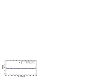
Figure 7: The masses of the pseudoscalar ($P$) and scalar ($S$) $B_{c}$ mesons with variations of the Borel parameters $T^{2}$.

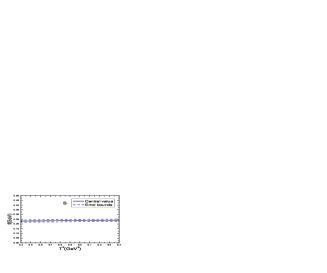
Figure 8: The pole residues of the pseudoscalar ($P$) and scalar ($S$) $B_{c}$ mesons with variations of the Borel parameters $T^{2}$.

While the decay constants, even for the pseudoscalar $B_{c}$ meson, the theoretical values vary in a large range, for example, $f_{P}=460\pm 60\,\rm{MeV}$ [16], $300\pm 65\,\rm{MeV}$ [36], $360\pm 60\,\rm{MeV}$ [37], $270\pm 30\,\rm{MeV}$ [41], $371\pm 17\,\rm{MeV}$ [43], $528\pm 19\,\rm{MeV}$ [44] from the full QCD sum rules, $410\pm 40\,\rm{MeV}$ [11], $433\,\rm{MeV}$ [12] from the relativistic quark model, $498\,\rm{MeV}$ [18], $440\,\rm{MeV}$ [19] from the non-relativistic quark model, $523\pm 62\,\rm{MeV}$ [54] from the light-front quark model, $420\pm 13\,\rm{MeV}$ [31] from the lattice non-relativistic QCD, $315^{+26}_{-50}\,\rm{MeV}$ [25] from the shifted $N$-expansion method, $438\pm 10\,\rm{MeV}$ [55] from the field correlator method, $322\pm 42\,\rm{MeV}$ [33] from the Bethe-Salpeter equation, etc. At the present time, it is difficult to say which value is superior to others.

The present calculation $f_{P}=371\pm 37\,\rm{MeV}$ is in very good agreement with the value $371\pm 17\,\rm{MeV}$ from the full QCD sum rules [43]. In our previous work, we obtain the values $f_{V}=384\pm 32\,\rm{MeV}$ and $f_{A}=373\pm 25\,\rm{MeV}$ for the vector and axial-vector $B_{c}$ mesons, respectively. Our calculations indicate that $f_{P}\approx f_{V}\approx f_{A}>f_{S}$. While in the QCD sum rule combined with the heavy quark effective theory up to the order $\alpha_{s}^{3}$, the decay constants have the relations $\tilde{f}_{P}=f_{P}>f_{V}>f_{S}>\tilde{f}_{S}>f_{A}$ [47], where the decay constants $\tilde{f}_{P}$ and $\tilde{f}_{S}$ are defined by

$$\langle 0|J_{P}(0)|P(p)\rangle = \tilde{f}_{P}M_{P}\,,$$

$$\langle 0|J_{S}(0)|S(p)\rangle = \tilde{f}_{S}M_{S}\,.$$ (25)

From Eq.(2) and Eq.(3), we can obtain the relations,

$$\tilde{f}_{P} = f_{P}\frac{M_{P}}{m_{b}+m_{c}}\,,$$

$$\tilde{f}_{S} = f_{S}\frac{M_{S}}{m_{b}-m_{c}}\,,$$ (26)

it is obvious that $\tilde{f}_{P}>f_{P}$ and $\tilde{f}_{S}<f_{S}$, which are in contrary to the relations obtained in Ref.[47], so no definite conclusion can be obtained. Naively, we expect that the vector mesons have larger decay constants than the corresponding pseudoscalar mesons [59].

The leptonic decay widths $\Gamma_{\ell\bar{\nu}_{\ell}}$ of the pseudoscalar and scalar $B_{c}$ mesons can be written as,

$$\Gamma_{\ell\bar{\nu}_{\ell}} = \frac{G_{F}^{2}}{8\pi}|V_{bc}|^{2}f_{P/S}^{2}M_{P/S}M_{\ell}^{2}\left(1-\frac{M_{\ell}^{2}}{M_{P/S}^{2}}\right)^{2}\,,$$ (27)

where $\ell=e,\mu,\tau$, the Fermi constant $G_{F}=1.16637\times 10^{-5}\,\rm{GeV}^{-2}$, the CKM matrix element $V_{cb}=40.8\times 10^{-3}$, the masses of the leptons $m_{e}=0.511\times 10^{-3}\,\rm{GeV}$, $m_{\mu}=105.658\times 10^{-3}\,\rm{GeV}$, $m_{\tau}=1776.86\times 10^{-3}\,\rm{GeV}$, the life time of the $B_{c}$ meson $\tau_{B_{c}}=0.510\times 10^{-12}\,s$ [5]. We take the masses and decay constants of the pseudoscalar and scalar $B_{c}$ mesons from the QCD sum rules to obtain the partial decay widths,

$$\Gamma_{P\to e\bar{\nu}_{e}} = 2.03\times 10^{-12}\,\rm{eV}\,,$$

$$\Gamma_{P\to\mu\bar{\nu}_{\mu}} = 8.68\times 10^{-8}\,\rm{eV}\,,$$

$$\Gamma_{P\to\tau\bar{\nu}_{\tau}} = 2.08\times 10^{-5}\,\rm{eV}\,,$$

$$\Gamma_{S\to e\bar{\nu}_{e}} = 8.78\times 10^{-13}\,\rm{eV}\,,$$

$$\Gamma_{S\to\mu\bar{\nu}_{\mu}} = 3.75\,\times 10^{-8}\,\rm{eV}\,,$$

$$\Gamma_{S\to\tau\bar{\nu}_{\tau}} = 9.18\,\times 10^{-6}\,\rm{eV}\,,$$ (28)

and the branching fractions,

$${\rm Br}_{P\to e\bar{\nu}_{e}} = 1.57\times 10^{-9}\,,$$

$${\rm Br}_{P\to\mu\bar{\nu}_{\mu}} = 6.73\times 10^{-5}\,,$$

$${\rm Br}_{P\to\tau\bar{\nu}_{\tau}} = 1.61\times 10^{-2}\,.$$ (29)

The largest branching fractions of the $B_{c}(0^{-})\to\ell\bar{\nu}_{\ell}$ are of the order $10^{-2}$, the tiny branching fractions maybe escape experimental detections.

4 Conclusion

In this work, we extend our previous works on the vector and axialvector $B_{c}$ mesons to investigate the pseudoscalar and scalar $B_{c}$ mesons with the full QCD sum rules by including next-to-leading order corrections and choose the updated input parameters. In calculating the next-to-leading order corrections, we use optical theorem to obtain the spectral densities directly, and resort to the scheme of the dimensional regularization to regularize both the ultraviolet and infrared divergences, which are canceled out with each other separately, the net spectral densities are free of divergences. We take the experimental data as guides to choose the suitable Borel parameters and continuum threshold parameters, and make reasonable predictions for the masses and decay constants, therefore the pure leptonic decay widths, which can be confronted to the experimental data in the future.

Appendix

Firstly, we write down the fundamental integrals in calculating the vertex corrections,

$$V_{ab}(s) = 16\pi^{2}\int_{0}^{1}dx\int_{0}^{1-x}dy\int\frac{d^{D}k_{E}}{(2\pi)^{D}}\frac{x^{a}y^{b}\Gamma(3)}{\left[k^{2}_{E}+(xp_{1}+yp_{2})^{2}\right]^{3}}\,,$$

$$V(s) = 16\pi^{2}\left(1-\frac{1}{2}\varepsilon_{\rm UV}\right)\int_{0}^{1}dx\int_{0}^{1-x}dy\int\frac{d^{D}k_{E}}{(2\pi)^{D}}\frac{k^{2}_{E}\Gamma(3)}{\left[k^{2}_{E}+(xp_{1}+yp_{2})^{2}\right]^{3}}\,,$$ (30)

and carry out the integrals to obtain the analytical expressions,

$$V_{00}(s) = \frac{1}{\sqrt{\lambda(s,m_{b}^{2},m_{c}^{2})}}\left\{-\log\left(\frac{1+\omega}{1-\omega}\right)\left(\frac{1}{\varepsilon_{\rm IR}}+\log\frac{s}{4\pi\mu^{2}}+\gamma\right)+\frac{\log^{2}(1-\omega_{1}^{2})}{4}-\log^{2}(1+\omega_{1})\right.$$

$$+\frac{\log^{2}(1-\omega_{2}^{2})}{4}-\log^{2}(1+\omega_{2})+2\log(\omega_{1}+\omega_{2})\log\left(\frac{1+\omega}{1-\omega}\right)-\log\omega_{1}\log\left(\frac{1+\omega_{2}}{1-\omega_{2}}\right)$$

$$\left.-\log\omega_{2}\log\left(\frac{1+\omega_{1}}{1-\omega_{1}}\right)-{\rm Li_{2}}\left(\frac{2\omega_{1}}{1+\omega_{1}}\right)-{\rm Li_{2}}\left(\frac{2\omega_{2}}{1+\omega_{2}}\right)+\pi^{2}\right\}\,,$$

$$= \overline{V}_{00}(s)-\frac{1}{\sqrt{\lambda(s,m_{b}^{2},m_{c}^{2})}}\log\left(\frac{1+\omega}{1-\omega}\right)\left(\frac{1}{\varepsilon_{\rm IR}}+\log\frac{s}{4\pi\mu^{2}}+\gamma\right)\,,$$

$$V_{10}(s) = \frac{1}{s}\left\{\frac{1}{2}\log\left(\frac{1-\omega_{1}^{2}}{1-\omega_{2}^{2}}\right)-\frac{1}{\omega_{2}}\log\left(\frac{1+\omega}{1-\omega}\right)+\log\frac{\omega_{2}}{\omega_{1}}\right\}\,,$$

$$V_{01}(s) = V_{10}(s)|_{\omega_{1}\leftrightarrow\omega_{2}}\,,$$

$$V_{20}(s) = \frac{1}{2s}\left\{-\frac{\omega_{1}\omega_{2}}{\omega_{1}+\omega_{2}}\log\left(\frac{1+\omega}{1-\omega}\right)-\frac{\omega_{1}}{\omega_{2}(\omega_{1}+\omega_{2})}\log\left(\frac{1+\omega}{1-\omega}\right)+\frac{\omega_{1}}{\omega_{1}+\omega_{2}}\log\left(\frac{1-\omega_{1}^{2}}{1-\omega_{2}^{2}}\right)\right.$$

$$\left.+\frac{2\omega_{1}}{\omega_{1}+\omega_{2}}\log\frac{\omega_{2}}{\omega_{1}}+1\right\}\,,$$

$$V_{02}(s) = V_{20}(s)|_{\omega_{1}\leftrightarrow\omega_{2}}\,,$$

$$V_{11}(s) = \frac{1}{2s}\left\{\frac{\omega_{1}\omega_{2}}{\omega_{1}+\omega_{2}}\log\left(\frac{1+\omega}{1-\omega}\right)-\frac{\omega_{1}-\omega_{2}}{2(\omega_{1}+\omega_{2})}\log\left(\frac{1-\omega_{1}^{2}}{1-\omega_{2}^{2}}\right)-\frac{1}{\omega_{1}+\omega_{2}}\log\left(\frac{1+\omega}{1-\omega}\right)\right.$$

$$\left.+\frac{\omega_{1}}{\omega_{1}+\omega_{2}}\log\frac{\omega_{1}}{\omega_{2}}+\frac{\omega_{2}}{\omega_{1}+\omega_{2}}\log\frac{\omega_{2}}{\omega_{1}}-1\right\}\,,$$

$$V(s) = \frac{1}{\varepsilon_{\rm UV}}+\log\frac{4\pi\mu^{2}}{s}-\gamma+2-\frac{2\omega_{1}\omega_{2}}{\omega_{1}+\omega_{2}}\log\left(\frac{1+\omega}{1-\omega}\right)-\frac{\omega_{2}}{\omega_{1}+\omega_{2}}\log(1-\omega_{1}^{2})$$ (31)

$$-\frac{\omega_{1}}{\omega_{1}+\omega_{2}}\log(1-\omega_{2}^{2})-2\frac{\omega_{1}\log\omega_{1}+\omega_{2}\log\omega_{2}}{\omega_{1}+\omega_{2}}+2\log(\omega_{1}+\omega_{2})\,,$$

$$= \overline{V}(s)+\frac{1}{\varepsilon_{\rm UV}}+\log\frac{4\pi\mu^{2}}{s}-\gamma+2\,,$$

where

$$\omega_{1} = \frac{\sqrt{\lambda(s,m_{b}^{2},m_{c}^{2})}}{s+m_{b}^{2}-m_{c}^{2}}\,,$$

$$\omega_{2} = \frac{\sqrt{\lambda(s,m_{b}^{2},m_{c}^{2})}}{s+m_{c}^{2}-m_{b}^{2}}\,,$$

$$M = \frac{m_{b}+m_{c}}{m_{b}-m_{c}}\,,$$

$${\rm Li_{2}}(x) = -\int_{0}^{x}dt\frac{\log(1-t)}{t}\,.$$ (32)

Secondly, we introduce the notation

$$\int dps = \int\frac{d^{D-1}\vec{k}}{2E_{k}}\frac{d^{D-1}\vec{p}_{1}}{2E_{p_{1}}}\frac{d^{D-1}\vec{p}_{2}}{2E_{p_{2}}}\delta^{D}(p-k-p_{1}-p_{2})\,,$$

for simplicity, and write down the analytical expressions of the three-body phase-space integrals,

$$R_{11}(s) = \frac{sm_{b}^{2}}{\pi^{2}\sqrt{\lambda(s,m_{b}^{2},m_{c}^{2})}}(2\pi)^{-4\varepsilon_{\rm IR}}\mu^{-2\varepsilon_{\rm IR}}\int dps\frac{1}{(k\cdot p_{1})^{2}}$$

$$= \frac{1}{2\varepsilon_{\rm IR}}-\log 4\pi+\gamma-1+\log\frac{\sqrt{\lambda(s,m_{b}^{2},m_{c}^{2})}^{3}}{m_{b}m_{c}s\mu^{2}}-\frac{s+m_{b}^{2}-m_{c}^{2}}{2\sqrt{\lambda(s,m_{b}^{2},m_{c}^{2})}}\log\left(\frac{1+\omega_{1}}{1-\omega_{1}}\right)$$

$$-\frac{m_{b}^{2}-m_{c}^{2}}{\sqrt{\lambda(s,m_{b}^{2},m_{c}^{2})}}\log\left(\frac{1+\omega_{1}}{1-\omega_{1}}\right)-\frac{s-m_{b}^{2}+m_{c}^{2}}{\sqrt{\lambda(s,m_{b}^{2},m_{c}^{2})}}\log\left(\frac{1+\omega}{1-\omega}\right)$$

$$= \overline{R}_{11}(s)+\frac{1}{2\varepsilon_{\rm IR}}-\log 4\pi+\gamma-1+\log\frac{\sqrt{\lambda(s,m_{b}^{2},m_{c}^{2})}^{3}}{m_{b}m_{c}s\mu^{2}}\,,$$

$$R_{22}(s) = R_{11}(s)|_{m_{b}\leftrightarrow m_{c}}\,,$$

$$R_{12}(s) = \frac{s}{\pi^{2}\sqrt{\lambda(s,m_{b}^{2},m_{c}^{2})}}(2\pi)^{-4\varepsilon_{\rm IR}}\mu^{-2\varepsilon_{\rm IR}}\int dps\frac{1}{k\cdot p_{1}k\cdot p_{2}}$$

$$= \frac{1}{\sqrt{\lambda(s,m_{b}^{2},m_{c}^{2})}}\left\{\log\left(\frac{1+\omega}{1-\omega}\right)\left[\frac{1}{\varepsilon_{\rm IR}}-2\log 4\pi+2\gamma-2+2\log\frac{\sqrt{\lambda(s,m_{b}^{2},m_{c}^{2})}^{3}}{m_{b}m_{c}s\mu^{2}}\right]\right.$$

$$-2\log\frac{m_{b}}{m_{c}}\log\left(\frac{M+\omega}{M-\omega}\right)-\log^{2}\left(\frac{1+\omega}{1-\omega}\right)+2\log\frac{s}{\bar{s}}\log\left(\frac{1+\omega}{1-\omega}\right)-4{\rm Li_{2}}\left(\frac{2\omega}{1+\omega}\right)$$

$$+2{\rm Li_{2}}\left(\frac{\omega-1}{\omega-M}\right)+2{\rm Li_{2}}\left(\frac{\omega-1}{\omega+M}\right)-2{\rm Li_{2}}\left(\frac{\omega+1}{\omega-M}\right)-2{\rm Li_{2}}\left(\frac{\omega+1}{\omega+M}\right)-\frac{1}{2}{\rm Li_{2}}\left(\frac{1+\omega_{1}}{2}\right)$$

$$\left.-\frac{1}{2}{\rm Li_{2}}\left(\frac{1+\omega_{2}}{2}\right)-{\rm Li_{2}}\left(\omega_{1}\right)-{\rm Li_{2}}\left(\omega_{2}\right)+\frac{\log 2\log\left[(1+\omega_{1})(1+\omega_{2})\right]}{2}-\frac{\log^{2}2}{2}+\frac{\pi^{2}}{12}\right\}\,,$$

$$= \overline{R}_{12}(s)+\frac{1}{\sqrt{\lambda(s,m_{b}^{2},m_{c}^{2})}}\log\left(\frac{1+\omega}{1-\omega}\right)\left[\frac{1}{\varepsilon_{\rm IR}}-2\log 4\pi+2\gamma-2+2\log\frac{\sqrt{\lambda(s,m_{b}^{2},m_{c}^{2})}^{3}}{m_{b}m_{c}s\mu^{2}}\right]\,,$$

$$R^{1}_{12}(s) = \frac{s}{\pi^{2}\sqrt{\lambda(s,m_{b}^{2},m_{c}^{2})}}\int dps\frac{s-K^{2}}{k\cdot p_{1}k\cdot p_{2}}$$

$$= \frac{s}{\sqrt{\lambda(s,m_{b}^{2},m_{c}^{2})}}\left\{\log^{2}(1-\omega)-\log^{2}(1+\omega)+2\log\frac{2s}{\bar{s}}\log\left(\frac{1+\omega}{1-\omega}\right)+2{\rm Li_{2}}\left(\frac{1-\omega}{2}\right)\right.$$

$$\left.-2{\rm Li_{2}}\left(\frac{1+\omega}{2}\right)+2{\rm Li_{2}}\left(\frac{1+\omega}{1+M}\right)+2{\rm Li_{2}}\left(\frac{1+\omega}{1-M}\right)-2{\rm Li_{2}}\left(\frac{1-\omega}{1-M}\right)-2{\rm Li_{2}}\left(\frac{1-\omega}{1+M}\right)\right\}\,,$$

$$R^{2}_{12}(s) = \frac{s}{\pi^{2}\sqrt{\lambda(s,m_{b}^{2},m_{c}^{2})}}\int dps\frac{\left(s-K^{2}\right)^{2}}{k\cdot p_{1}k\cdot p_{2}}$$ (33)

$$= \frac{s^{2}}{\sqrt{\lambda(s,m_{b}^{2},m_{c}^{2})}}\left\{\log^{2}(1-\omega)-\log^{2}(1+\omega)+2\log\frac{4s}{\bar{s}}\log\left(\frac{1+\omega}{1-\omega}\right)+2{\rm Li_{2}}\left(\frac{1-\omega}{2}\right)\right.$$

$$-2{\rm Li_{2}}\left(\frac{1+\omega}{2}\right)+2{\rm Li_{2}}\left(\frac{1+\omega}{1+M}\right)+2{\rm Li_{2}}\left(\frac{1+\omega}{1-M}\right)-2{\rm Li_{2}}\left(\frac{1-\omega}{1-M}\right)-2{\rm Li_{2}}\left(\frac{1-\omega}{1+M}\right)\,$$

$$\left.+\frac{2\omega\bar{s}}{s}-\frac{\bar{s}}{s}(1+\omega^{2})\log\left(\frac{1+\omega}{1-\omega}\right)\right\}\,,$$

where $\bar{s}=s-(m_{b}-m_{c})^{2}$.

References

• [1] F. Abe et al, Phys. Rev. D58 (1998) 112004.
• [2] F. Abe et al, Phys. Rev. Lett. 81 (1998) 2432.
• [3] T. Aaltonen et al, Phys. Rev. Lett. 100 (2008) 182002.
• [4] V. M. Abazov et al, Phys. Rev. Lett. 101 (2008) 012001.
• [5] R. L. Workman et al, Prog. Theor. Exp. Phys. 2022 (2022) 083C01.
• [6] G. Aad et al, Phys. Rev. Lett. 113 (2014) 212004.
• [7] A. M. Sirunyan et al, Phys. Rev. Lett. 122 (2019) 132001.
• [8] R. Aaij et al, Phys. Rev. Lett. 122 (2019) 232001.
• [9] Z. G. Wang, Eur. Phys. J. C73 (2013) 2559.
• [10] S. Godfrey and N. Isgur, Phys. Rev. D32 (1985) 189.
• [11] S. Godfrey, Phys. Rev. D70 (2004) 054017.
• [12] D. Ebert, R. N. Faustov and V. O. Galkin, Phys. Rev. D67 (2003) 014027.
• [13] S. N. Gupta and J. M. Johnson, Phys. Rev. D53 (1996) 312.
• [14] J. Zeng, J. W. Van Orden and W. Roberts, Phys. Rev. D52 (1995) 5229.
• [15] S. S. Gershtein, V. V. Kiselev, A. K. Likhoded and A. V. Tkabladze, Phys. Rev. D51 (1995) 3613.
• [16] S. S. Gershtein, V. V. Kiselev, A. K. Likhoded and A. V. Tkabladze, Phys. Usp. 38 (1995) 1.
• [17] E. J. Eichten and C. Quigg, Phys. Rev. D49 (1994) 5845.
• [18] E. J. Eichten and C. Quigg, Phys. Rev. D99 (2019) 054025.
• [19] A. P. Monteiro, M. Bhat and K. B. V. Kumar, Int. J. Mod. Phys. A32 (2017) 1750021.
• [20] L. P. Fulcher, Phys. Rev. D60 (1999) 074006.
• [21] N. R. Soni, B. R. Joshi, R. P. Shah, H. R. Chauhan and J. N. Pandya, Eur. Phys. J. C78 (2018) 592.
• [22] P. G. Ortega, J. Segovia, D. R. Entem and F. Fernandez, Eur. Phys. J. C80 (2020) 223.
• [23] Q. Li, M. S. Liu, L. S. Lu, Q. F. Lu, L. C. Gui and X. H. Zhong, Phys. Rev. D99 (2019) 096020.
• [24] S. M. Ikhdair and R. Sever, Int. J. Mod. Phys. A19 (2004) 1771.
• [25] S. M. Ikhdair and R. Sever, Int. J. Mod. Phys. A21 (2006) 6699.
• [26] N. Brambilla and A. Vairo, Phys. Rev. D62 (2000) 094019.
• [27] A. A. Penin, A. Pineda, V. A. Smirnov and M. Steinhauser, Phys. Lett. B593 (2004) 124.
• [28] E. B. Gregory et al, Phys. Rev. Lett. 104 (2010) 022001.
• [29] C. T. H. Davies et al, Phys. Lett. B382 (1996) 131.
• [30] N. Mathur, M. Padmanath and S. Mondal, Phys. Rev. Lett. 121 (2018) 202002.
• [31] B. D. Jones and R. M. Woloshyn, Phys. Rev. D60 (1999) 014502.
• [32] A. A. EI-Hady, M. A. K. Lodhi and J. P. Vary, Phys. Rev. D59 (1999) 094001.
• [33] G. L. Wang, Phys. Lett. B650 (2007) 15.
• [34] G. L. Wang, T. Wang, Q. Li and C. H. Chang, JHEP 05 (2022) 006.
• [35] E. Bagan, H. G. Dosch, P. Gosdzinsky, S. Narison and J. M. Richard, Z. Phys. C64 (1994) 57.
• [36] M. Chabab, Phys. Lett. B325 (1994) 205.
• [37] P. Colangelo, G. Nardulli and N. Paver, Z. Phys. C57 (1993) 43.
• [38] V. V. Kiselev and A. V. Tkabladze, Phys. Rev. D48 (1993) 5208.
• [39] Z. G. Wang, Acta Phys. Polon. B44 (2013) 1971.
• [40] Z. G. Wang, Eur. Phys. J. A49 (2013) 131.
• [41] T. M. Aliev, T. Barakat and S. Bilmis, Nucl. Phys. B947 (2019) 114726.
• [42] M. Blanke et al, Phys. Rev. D99 (2019) 075006.
• [43] S. Narison, Phys. Lett. B802 (2020) 135221.
• [44] M. J. Baker, J. Bordes, C. A. Dominguez, J. Penarrocha and K. Schilcher, JHEP 07 (2014) 032.
• [45] A. I. Onishchenko and O. L. Veretin, Eur. Phys. J. C50 (2007) 801.
• [46] J. Lee, W. L. Sang and S. Kim, JHEP 01 (2011) 113.
• [47] W. Tao and Z. J. Xiao, arXiv: 2310.17500 [hep-ph].
• [48] W. Tao, R. L. Zhu and Z. J. Xiao, Phys. Rev. D106 (2022) 114037.
• [49] W. Tao, R. L. Zhu and Z. J. Xiao, Eur. Phys. J. C83 (2023) 294.
• [50] L. B. Chen and C. F. Qiao, Phys. Lett. B748 (2015) 443.
• [51] W. L. Sang, H. F. Zhang and M. Z. Zhou, Phys. Lett. B839 (2023) 137812.
• [52] F. Feng, Y. Jia, Z. Mo, J. Pan, W. L. Sang and J. Y. Zhang, arXiv: 2208.04302 [hep-ph].
• [53] R. C. Verma, J. Phys. G39 (2012) 025005.
• [54] S. Tang, Y. Li, P. Maris and J. P. Vary, Phys. Rev. D98 (2018) 114038.
• [55] A. M. Badalian, B. L. G. Bakker and Yu. A. Simonov, Phys. Rev. D75 (2007) 116001.
• [56] L. J. Reinders, H. Rubinstein and S. Yazaki, Phys. Rept. 127 (1985) 1.
• [57] T. D. Lee and M. Nauenberg, Phys. Rev. 133 (1964) B1549.
• [58] S. Narison, Phys. Lett. B706 (2012) 412.
• [59] Z. G. Wang, Eur. Phys. J. C75 (2015) 427.