Magnetic Dirac systems: Violation of bulk-edge correspondence in the zigzag limit

Abstract.

We consider a Dirac operator with constant magnetic field defined on a half-plane with boundary conditions that interpolate between infinite mass and zigzag. By a detailed study of the energy dispersion curves we show that the infinite mass case generically captures the profile of these curves, which undergoes a continuous pointwise deformation into the topologically different zigzag profile. Moreover, these results are applied to the bulk-edge correspondence. In particular, by means of a counterexample, we show that this correspondence does not always hold true in the zigzag case.

1. Introduction and main results

Bulk-edge correspondence is a notion that arises in the study of certain condensed matter physics systems possessing non-trivial topology. It establishes a connection between the bulk properties of a material (its interior or bulk region) and its edge or boundary properties. This correspondence may be given through an equation that links a Chern number, that depends only on the bulk operator, and an expression involving the edge-states localized close to the boundary; eventually yielding the so-called topological quantization of edge currents [13]. Due to the integer (or topological) nature of the Chern number these relations are very stable under smooth changes of the material parameters and therefore its importance for potential applications. In this context, Dirac Hamiltonians are prominent examples that exhibit interesting phenomena. They are used to model various materials, among them, graphene and topological insulators [14].

In this article we investigate the bulk-edge correspondence for a two-dimensional Dirac Hamiltonian with a constant magnetic field defined on a half-plane. This model was recently considered in [6], where bulk-edge correspondence was shown to hold, provided infinite-mass boundary conditions along the edge are imposed. Our motivation is to investigate the validity of these results when any fixed admissible local boundary condition is allowed. To this end we define a family of Dirac Hamiltonians $\mathscr{D}_{\gamma}$, where $\gamma\in\mathbb{R}\cup\{+\infty\}$ characterizes the boundary conditions, in particular, $\gamma=\pm 1$ corresponds to infinite mass.

Our main result Theorem 1.2 indicates that bulk-edge correspondence for this model still holds, provided the boundary conditions are not zigzag (i.e. $\gamma\notin\{0,+\infty\}$). Moreover, Theorem 1.2 shows that this correspondence is violated for certain energies when zigzag boundary conditions are imposed. In order to show Theorem 1.2 certain knowledge on the energy dispersion curves associated to $\mathscr{D}_{\gamma}$ is helpful. In this work we present a fairly detailed analysis of them extending the results of [3] to any local boundary condition. We complement our analysis with numerical illustrations of the energy dispersion curves for different values of the boundary parameter and the magnetic field.

Let us now turn to define our model. We consider a magnetic Dirac system on the half-plane denoted by $\mathbb{R}^{2}_{+}=\{(x_{1},x_{2})\in\mathbb{R}^{2}:x_{2}>0\}$ in the presence of an orthogonal magnetic field whose component in the $x_{3}$ direction is given by $b\in\mathbb{R}\setminus\{0\}$. The corresponding Hamiltonian acts on functions in $L^{2}(\mathbb{R}^{2}_{+},\mathbb{C}^{2})$ as

$$\sigma\cdot(-i\nabla-\mathbf{A})=\begin{pmatrix}0&-i\partial_{1}-\partial_{2}+bx_{2}\\ -i\partial_{1}+\partial_{2}+bx_{2}&0\end{pmatrix}\,.$$ (1.1)

Here $\mathbf{A}$ refers to a vector potential associated with the magnetic field i.e. $\rm{rot}\mathbf{A}=b{\rm e}_{3}$. We choose

$$\mathbf{A}=(-bx_{2},0)\,.$$

We recall that

$$\sigma_{1}=\begin{pmatrix}0&1\\ 1&0\end{pmatrix}\,,\quad\sigma_{2}=\begin{pmatrix}0&-i\\ i&0\end{pmatrix}\,,\quad\sigma_{3}=\begin{pmatrix}1&0\\ 0&-1\end{pmatrix}\,.$$

The study of the magnetic Dirac operator on the half-plane with infinite mass boundary conditions was recently carried forward in [3]. Here we consider general local conditions at the edge interpolating between zigzag and infinite mass. More precisely: Let $\gamma\in\mathbb{R}\cup\{+\infty\}$, then we consider the self-adjoint realization $\mathscr{D}_{\gamma}\equiv\mathscr{D}_{\gamma}(b)$ acting as (1.1) on a subset of functions $\psi=(\psi_{1},\psi_{2})\in L^{2}(\mathbb{R}^{2}_{+},\mathbb{C}^{2})$ satisfying, for all $x_{1}\in\mathbb{R}$,

$$\begin{cases}\psi_{2}(x_{1},0)=\gamma\psi_{1}(x_{1},0)&\text{ if }\gamma\in\mathbb{R}\,,\\ \psi_{1}(x_{1},0)=0&\text{ if }\gamma=+\infty\,.\end{cases}$$ (1.2)

The two cases $\gamma\in\{0,+\infty\}$ are called zigzag, while $\gamma=\pm 1$ corresponds to infinite mass boundary conditions (see Remark 1.3 bellow).

Remark 1.1.

The domains of self-adjointness of the operators $\mathscr{D}_{\gamma}$ are already known: See [3, Section 1C] for the zigzag cases and [3, Theorem 1.15] for the infinite mass; the latter result can be easily adapted for the non-zigzag cases. For the essential self-adjointness of $\mathscr{D}_{\gamma}$ on the class of Schwartz functions with infinite mass boundary conditions see [6, Proposition 1.1], and for the general case see [1].

We denote by $X_{1}$ the operator of multiplication with $x_{1}$, and by $J_{1}$ the current density operator, we have

$$J_{1}=-i[\mathscr{D}_{\gamma},X_{1}]=-\sigma_{1}\,.$$

Recall that the Landau Hamiltonian $\mathscr{D}_{bulk}(b)$ acts on the whole plane as in (1.1) and its spectrum consists of the Landau levels given by $\{\pm\sqrt{2n|b|},\,n\in\mathbb{N}_{0}\}$.

We say that $F:\mathbb{R}\to\mathbb{R}$ is equal to $a\in\mathbb{R}$ near $x_{0}\in\mathbb{R}$ if there exists an open interval $I$ around $x_{0}$ where $F(x)=a,x\in I,$ holds.

Our main result is the following.

Theorem 1.2.

Let $b>0$ and let $\chi=\mathds{1}_{(0,1)}$ be the indicator function of the interval $(0,1)$. Let $\gamma\in\mathbb{R}\cup\{+\infty\}$. Let $F\in C_{0}^{2}(\mathbb{R})$ be such that it equals $1$ near $n\geqslant 1$ Landau levels, and $0$ near the others. Then, the operator $\chi(X_{1})J_{1}F^{\prime}(\mathscr{D}_{\gamma})$ is trace class and the edge Hall conductance is given by

$$\begin{split}2\pi\mathrm{Tr}\big{(}\chi(X_{1})J_{1}F^{\prime}(\mathscr{D}_{\gamma})\big{)}&=\begin{cases}n-1&\text{ if }\gamma=0\text{ and }F\text{ equals }1\text{ near }0\,,\\ n+1&\text{ if }\gamma=+\infty\text{ and }F\text{ equals }1\text{ near }0\,,\\ n&\text{otherwise}\,.\end{cases}\end{split}$$ (1.3)

Comments:

1. The fact that the left hand side of this formula can be interpreted as an edge conductance is explained for instance in [10].

2. Let us make the connection with the bulk-edge correspondence. Let $F$ and $n$ be as in Theorem 1.2 and define the orthogonal projection $P_{n}=F(\mathscr{D}_{bulk}(b))$. In our case, $P_{n}$ contains exactly $n$ bulk Landau levels and one can show that its Chern number equals $n$, which encapsulates the non-trivial topology of the bulk projection (see e.g. [6]). On the other hand, since $F^{\prime}$ equals $0$ near the Landau levels, $F^{\prime}(\mathscr{D}_{\gamma})$ only selects edge-states.

3. If $b<0$, the Chern number of $P_{n}$ becomes $-n$, and the right hand side of formula (1.3) must be multiplied by $-1$.

4. Our third alternative in (1.3) indicates that the bulk-edge correspondence should hold for all non-zigzag conditions, a result which in our case is confirmed by brute force, i.e. by direct computation and comparison with the bulk Chern number. The general proof of this fact, under more general conditions than purely constant magnetic field, will be considered in [1]. At least for $\gamma=1$, this has been shown to be the case [6]; for Schrödinger-like operators see [7].

5. If we work with zigzag boundary conditions, and if the zero-energy bulk Landau level belongs to the projection $P_{n}$, then one of the first two alternatives in (1.3) occurs. Thus the bulk-edge correspondence does not hold in this case. Such an anomaly has been previously observed in other continuous models such as shallow-water waves [11, 18], and for "regularized" non-magnetic Dirac-like operators [18]. The latter are in fact second order differential operators, with boundary conditions that are incompatible with first-order self-adjoint differential operators.

Remark 1.3 (On the boundary condition).

General local boundary conditions for Dirac operators are usually written as $(-i\sigma_{3}(\sigma\cdot\mathbf{n})\cos\eta+\sigma_{3}\sin\eta)\psi=\psi,$ on $\partial\mathbb{R}^{2}_{+}\,,$ where $\eta\in\left[-\frac{\pi}{2},\frac{3\pi}{2}\right)$ (see e.g. [5] and [4, 3]). In the present situation, we have $\mathbf{n}=-e_{2}$ and thus

$$(\sigma_{1}\cos\eta+\sigma_{3}\sin\eta)\psi=\psi\,,\quad\text{ on }\partial\mathbb{R}^{2}_{+}\,.$$

We obtain (1.2) by setting $\gamma=\frac{\cos\eta}{1+\sin\eta}=\tan\left(\frac{\pi}{4}-\frac{\eta}{2}\right)$ with the convention $\gamma=+\infty$ in the case $\eta=-\pi/2$ i.e. $\psi_{1}=0$ on $\partial\mathbb{R}^{2}_{+}$.

1.1. The energy dispersion curves

Our proof of Theorem 1.2 requires certain knowledge on the energy dispersion curves and their corresponding eigenfunctions. In what follows we present a description of these curves for different values of the boundary parameter $\gamma$. The main technical issue here is the lack of semi-boundedness of $\mathscr{D}_{\gamma}$. This can however be treated using appropriate variational methods [12, 9, 16]; we follow the approach proposed in [3]. Before presenting our main results in this context we establish the basic framework.

1.1.1. Setting

In view of the translation invariance in the $x_{1}$-direction, we may use the partial Fourier transform to represent $\mathscr{D}_{\gamma}(b)$ as a family of fiber operators $\mathscr{D}_{\gamma,\xi}(b)\equiv\mathscr{D}_{\gamma,\xi}$, with $\xi\in\mathbb{R}$. Indeed, we have (see e.g. [3])

$$\mathscr{D}_{\gamma}=\int_{\mathbb{R}}^{\oplus}\mathscr{D}_{\gamma,\xi}\,{\rm d}\xi\,,$$

where the $1d$ magnetic Dirac operator $\mathscr{D}_{\gamma,\xi}$ acts as

$$\begin{pmatrix}0&d_{\xi}(b)\\ d^{\,\dagger}_{\xi}(b)&0\end{pmatrix}\equiv\begin{pmatrix}0&d_{\xi}\\ d^{\,\dagger}_{\xi}&0\end{pmatrix}\,,$$

with $d_{\xi}=\xi-\partial_{2}+bx_{2}$ and $d^{\,\dagger}_{\xi}=\xi+\partial_{2}+bx_{2}$. Its domain is given for $\gamma\notin\{0,+\infty\}$ as

$$\mathrm{Dom}(\mathscr{D}_{\gamma,\xi})=\{\psi\in H^{1}(\mathbb{R}_{+},\mathbb{C}^{2}):x_{2}\psi\in L^{2}(\mathbb{R}_{+})\,\,\,\mbox{and}\,\,\,\psi_{2}(0)=\gamma\psi_{1}(0)\}\,.$$ (1.4)

As for the zigzag cases, by denoting

$$B^{1}(\mathbb{R}_{+})=\{\psi\in H^{1}(\mathbb{R}_{+},\mathbb{C}^{2}):x_{2}\psi\in L^{2}(\mathbb{R}_{+})\}$$

we have

$$\mathrm{Dom}(\mathscr{D}_{0,\xi})=\{u\in L^{2}({\mathbb{R}_{+}}):d^{\,\dagger}_{\xi}u\in L^{2}(\mathbb{R}_{+})\}\times H_{0}^{1}(\mathbb{R}_{+})\cap B^{1}(\mathbb{R}_{+})\,,$$

$$\mathrm{Dom}(\mathscr{D}_{\infty,\xi})=H_{0}^{1}(\mathbb{R}_{+})\cap B^{1}(\mathbb{R}_{+})\times\{u\in L^{2}({\mathbb{R}_{+}}):d_{\xi}u\in L^{2}(\mathbb{R}_{+})\}\,.$$

We have that (cf. [3]), for any $\gamma\in\mathbb{R}\cup\{+\infty\}$ and $\xi\in\mathbb{R}$, the operator $\mathscr{D}_{\gamma,\xi}$ is self-adjoint and has compact resolvent (for $\gamma\not=\{0,+\infty\}$ it follows directly from the compact embedding of $H^{1}$ in $L^{2}$). We write the spectrum of $\mathscr{D}_{\gamma,\xi}$ as the set $\{-\vartheta_{j}^{-}(\gamma,\xi):j\in\mathbb{N}\}\cup\{\vartheta_{j}^{+}(\gamma,\xi):j\in\mathbb{N}\}$ such that

$$\ldots\leq-\vartheta_{2}^{-}(\gamma,\xi)\leq-\vartheta_{1}^{-}(\gamma,\xi)<0\leqslant\vartheta_{1}^{+}(\gamma,\xi)\leq\vartheta_{2}^{+}(\gamma,\xi)\leq\ldots$$ (1.5)

For a given boundary condition $\gamma\in\mathbb{R}\cup\{+\infty\}$ the map $\mathbb{R}\ni\xi\mapsto\vartheta_{n}^{\pm}(\gamma,\xi)$ defines the energy dispersion relation.

The following two propositions are shown in Section 3.1.

Proposition 1.4.

Let $\gamma\in\mathbb{R}\cup\{+\infty\}$ , $\xi\in\mathbb{R}$, $b\not=0$. We have

1. For all $n\geqslant 1$, the eigenvalues $\vartheta^{\pm}_{n}(\gamma,\xi)$ are simple.

2. For all $n\geqslant 1$, $\xi\mapsto\vartheta_{n}^{\pm}(\gamma,\xi)$ and $\gamma\mapsto\vartheta_{n}^{\pm}(\gamma,\xi)$ are real-analytic.

3. $0$ belongs to the spectrum of $\mathscr{D}_{\gamma,\xi}$ iff $\gamma=0$, in case $b>0$, or $\gamma=+\infty$, in case $b<0$ .

In order to study the zigzag case we introduce further the $1d$ fibers of a magnetic Dirichlet Pauli operator $\mathscr{H}_{\xi}(b)$ for $b>0$. It acts as $-\partial_{2}^{2}+(\xi+bx_{2})^{2}+b\,,$ with

$$\mathrm{Dom}(\mathscr{H}_{\xi}(b))=\{\psi\in H^{2}(\mathbb{R}_{+};\mathbb{C}):x_{2}^{2}\psi\in L^{2}(\mathbb{R}_{+})\,,\psi(0)=0\}\,.$$

It is well-known [8] that $\mathscr{H}_{\xi}(b)$ is self-adjoint with compact resolvent and that its spectrum consists on simple eigenvalues $(\nu_{n}^{\mathrm{Dir}}(b,\xi))_{n\in\mathbb{N}}$ with

$$2b<\nu_{1}^{\mathrm{Dir}}(b,\xi)<\nu_{2}^{\mathrm{Dir}}(b,\xi)<\ldots\,.$$

The following statements are well-known (see [17] and [2, 3]). We specialize in the case $b>0$ since otherwise one can use the charge conjugation symmetry described in Remark 1.9 below.

Proposition 1.5.

Consider the case $\gamma\in\{0,+\infty\}$. Then, for all $\xi\in\mathbb{R}$ and $b\not=0$, the spectrum of $\mathscr{D}_{\gamma,\xi}$ is symmetric with respect to $0$. Moreover, for $b>0$, we have

$$\begin{split}&\vartheta_{n}^{+}(+\infty,\xi)=\sqrt{\nu_{n}^{\mathrm{Dir}}(b,\xi)-2b}\quad(n\geqslant 1)\,,\end{split}$$

$$\begin{split}&\vartheta_{1}^{+}(0,\xi)=0,\,\,\,\mbox{and}\,\,\,\,\vartheta_{n}^{+}(0,\xi)=\sqrt{\nu_{n-1}^{\mathrm{Dir}}(b,\xi)}\quad(n\geqslant 2)\,.\end{split}$$

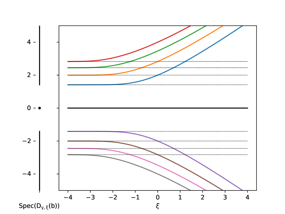
(a) Case $\gamma=0$: Here $0$ is an eigenvalue of $\mathscr{D}_{\gamma}$

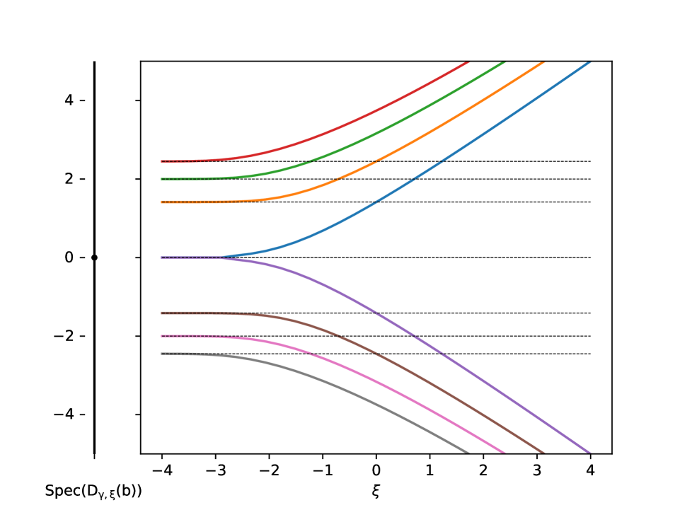
(b) Case $\gamma=\infty$: Here $0$ is not an eigenvalue. Dashed lines correspond to the Landau levels of the bulk operator.

Figure 1. Dispersion curves for the zigzag boundary conditions

Remark 1.6.

Recall [8] that, for $n\geqslant 1$, the function $\nu_{n}^{\mathrm{Dir}}(b,\cdot)$ is increasing and

$$\lim_{\xi\to-\infty}\nu_{n}^{\mathrm{Dir}}(b,\xi)=2nb\,,\quad\lim_{\xi\to+\infty}\nu_{n}^{\mathrm{Dir}}(b,\xi)=+\infty\,.$$

Figures 1(a) and 1(b) give the dispersion curves of the zigzag Dirac operators and on the left of each figure, their spectrum. All illustrations presented in this article are obtained thanks to standard finite difference schemes, inverse power and Newton-like methods.

1.1.2. Main results for the energy dispersion curves

In view of the symmetry it is enough to consider the cases of positive magnetic field and non-negative boundary parameter i.e. the case $(b,\gamma)\in(0,+\infty)\times[0,+\infty]$ (see Remark 1.9).

The following theorem gives a description of the dispersion curves when $\gamma\in(0,+\infty)$ and generalizes the result obtained in [3] for $\gamma=1$.

Theorem 1.7.

Let $\gamma\in(0,+\infty)$, $\xi\in\mathbb{R}$, $b>0$. The spectrum of $\mathscr{D}_{\gamma,\xi}(b)$ can be described as follows. Let $n\geqslant 1$.

1. The function $\vartheta^{+}_{n}(\gamma,\cdot)$ is increasing and

   $$\lim_{\xi\to-\infty}\vartheta^{+}_{n}(\gamma,\xi)=\sqrt{2(n-1)b}\,,\quad\lim_{\xi\to+\infty}\vartheta^{+}_{n}(\gamma,\xi)=+\infty\,.$$

2. The function $\vartheta^{-}_{n}(\gamma,\cdot)$ has a unique critical point, which is a non-degenerate minimum, and

   $$\lim_{\xi\to-\infty}\vartheta^{-}_{n}(\gamma,\xi)=\sqrt{2nb}\,,\quad\lim_{\xi\to+\infty}\vartheta^{-}_{n}(\gamma,\xi)=+\infty\,.$$ (1.6)

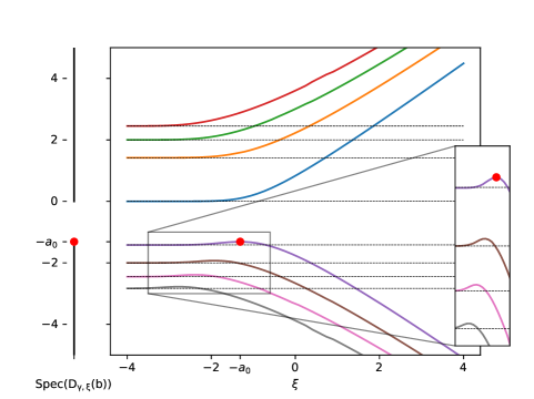
Figure 2. The dispersion curves of $\mathscr{D}_{\gamma,\xi}$ for $\gamma=b=1$

Figure 2 gives the dispersion curves of the infinite mass Dirac magnetic operator with a special focus on the global maxima of the negative dispersion curves. Here $a_{0}\in(0,\sqrt{2})$, was introduced in [3], it is the minimum of $\vartheta^{-}_{1}(1,\cdot)$, i.e., it is the size of the spectral gap of the Dirac operator with infinite mass boundary condition. The spectral gap of $\mathscr{D}_{\gamma}$ as a function of $\gamma$ can be read off from Figure 3.

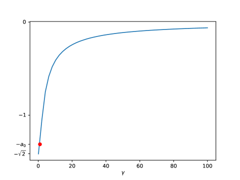
Figure 3. The value of the maximal negative energy of the full operator as a function of $\gamma$ for $b=1$.

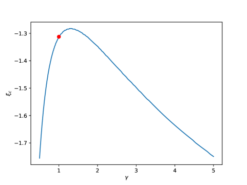
Figure 4. The location of the critical point of the first negative dispersion curve for $b=1$. The red bullet refers to $\gamma=1$.

Our next result describes the dispersion curves as functions of $\gamma$ and their zigzag limits.

Theorem 1.8.

Let $b>0$. The families of functions $[0,+\infty)\ni\gamma\mapsto\vartheta_{n}^{+}(\gamma,\cdot)$ and $[0,+\infty)\ni\gamma\mapsto-\vartheta_{n}^{-}(\gamma,\cdot)$ are increasing with $\gamma$. Moreover, for all $n\geqslant 1$ and all $\xi\in\mathbb{R}$, we have

$$\lim_{\gamma\to 0}\vartheta^{\pm}_{n}(\gamma,\xi)=\vartheta_{n}^{\pm}(0,\xi)\,,\quad\lim_{\gamma\to+\infty}\vartheta^{\pm}_{n}(\gamma,\xi)=\vartheta_{n}^{\pm}(+\infty,\xi)\,.$$

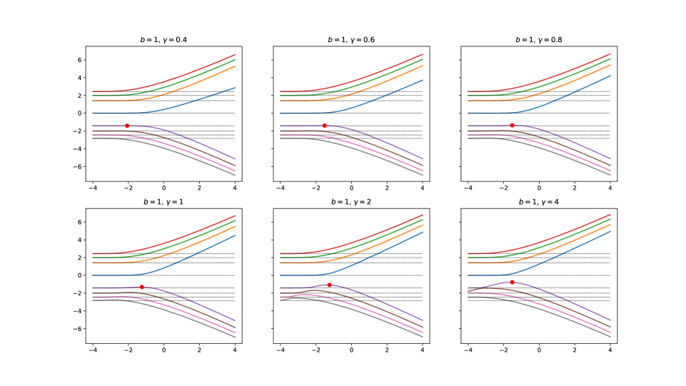
Figure 5. The dispersion curves for $b=1$ and various $\gamma$

In Figure 5 we present various pictures of the dispersion curves with varying $\gamma\in(0,+\infty)$. Moreover, Figure 6 illustrates the action of the symmetries, described in the following.

Remark 1.9 (Symmetries).

In view of the underlying symmetries it is enough to study the dispersion curves when $(b,\gamma)\in(0,+\infty)\times[0,+\infty]$. Indeed, in order to also consider $\gamma<0$, we notice that

$$\sigma_{3}\mathscr{D}_{\gamma}(b)=-\mathscr{D}_{-\gamma}(b)\sigma_{3}\,.$$

Moreover, for $b<0$ we used the charge conjugation $C\psi=\sigma_{1}\overline{\psi}$ which turns the boundary conditions into $\psi_{2}=\gamma^{-1}\psi_{1}$ and hence

$$C\mathscr{D}_{\gamma}(b)=-\mathscr{D}_{\gamma^{-1}}{(-b)}\,C\,.$$

For the fiber operators this leads to:

$$C\mathscr{D}_{\gamma,\xi}(b)=-\mathscr{D}_{\gamma^{-1},-\xi}(-b)\,C\,,\quad\sigma_{3}\,\mathscr{D}_{\gamma,\xi}(b)=-\mathscr{D}_{-\gamma,\xi}(b)\,\sigma_{3}\,.$$ (1.7)

In particular, we obtain the dispersion curves when $b<0$ from the curves when $b>0$ by changing $\gamma$ into $\gamma^{-1}$ and $\xi$ into $-\xi$.

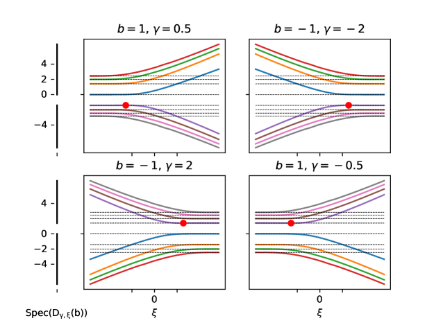
Figure 6. Action of the symmetries on the dispersion curves.

Organization of this article. In Section 2 we prove Theorem 1.2. Sections 3, 4, and 5 are devoted to the description of the energy dispersion relations $\vartheta_{n}^{\pm}(\gamma,\xi)$. In Section 3 we prove Propositions 1.4 and 1.5. In addition, we state in Theorem 3.5 a fixed-point characterization of $\vartheta_{n}^{\pm}(\gamma,\xi)$ in terms of a family $\big{(}\nu_{n}^{\pm}(\alpha,\xi)\big{)}_{\alpha>0}$ of the eigenvalues of certain magnetic Schrödinger-like operators with Robin boundary conditions. We give a proof of this characterization in Section 5. In Section 4 we investigate the fundamental mapping properties of $\nu_{n}^{\pm}(\alpha,\xi)$ for $\alpha>0$ and $\xi\in\mathbb{R}$. Finally, in Section 5, we apply Theorem 3.5, together with the analysis of Section 4, to prove Theorems 1.7 and 1.8.

2. Edge conductance formula

In this section we prove Theorem 1.2. In doing so we use various results on the energy dispersion curves which are stated in Section 1.1 and proved in the next sections.

We let, for all $j\geqslant 1$,

$$\lambda_{j}(\xi)=\vartheta^{+}_{j}(\gamma,\xi)\,,$$

and, for all $j\leqslant-1$,

$$\lambda_{j}(\xi)=-\vartheta^{-}_{j}(\gamma,\xi)\,.$$

Let $(\Psi_{\xi,j})_{\xi\in\mathbb{R}}$ be an analytic family of normalized eigenfunctions of $\mathscr{D}_{\gamma,\xi}$ associated with $\lambda_{j}(\xi)$ (see Proposition 1.4).

In view of the asymptotic behavior of $\lambda_{j}(\xi)$ as $\xi\to\pm\infty$ – stated in Theorem 1.7 (for the non-zigzag case) and Proposition 1.5 and Remark 1.6 (for the zigzag case) – the proof of Theorem 1.2 reduces to showing the following result.

Proposition 2.1.

We let $\chi=\mathds{1}_{(0,1)}$ and consider $\gamma\in\mathbb{R}\cup\{+\infty\}$. Let us consider a function $f\in C^{1}_{0}(\mathbb{R})$ being zero near the Landau levels. Then, the operator $\chi(X_{1})\sigma_{1}f(\mathscr{D}_{\gamma})$ is trace class and there exists a finite $J\subset\mathbb{Z}\setminus\{0\}$ such that

$$2\pi\mathrm{Tr}\big{(}\chi(X_{1})\sigma_{1}f(\mathscr{D}_{\gamma})\big{)}=\sum_{j\in J}\int_{\mathbb{R}}f(\lambda_{j}(\xi))\lambda^{\prime}_{j}(\xi)\mathrm{d}\xi\,.$$

In particular, if $n\in\mathbb{N}$ and $F\in C_{0}^{2}(\mathbb{R})$ equals $1$ near $n$ Landau levels and $0$ near the others, we have

$$-2i\pi\mathrm{Tr}\left(\chi(X_{1})[\mathscr{D}_{\gamma},X_{1}]F^{\prime}(\mathscr{D}_{\gamma})\right)=\sum_{j\in J}\Big{(}F\big{(}\lambda_{j}(-\infty)\big{)}-F\big{(}\lambda_{j}(+\infty)\big{)}\Big{)}\,.$$ (2.1)

Let us first state two useful elementary results. The first one is a direct consequence of Proposition 1.4 and Theorem 1.7.

Lemma 2.2.

Let us consider a function $f\in C_{0}(\mathbb{R})$ being zero near the Landau levels $\{\pm\sqrt{2n}\,,n\in\mathbb{N}\}$. Then, there exists a finite $J\subset\mathbb{Z}\setminus\{0\}$ such that for all $k\notin J$, $f\circ\lambda_{k}=0$ and for all $j\in J$, the functions $\xi\mapsto f(\lambda_{j}(\xi))$ have compact supports.

The following result might be elementary. We give its proof for the reader’s convenience.

Lemma 2.3.

Consider an operator $T$ on $L^{2}(\mathbb{R}^{2}_{+})$ given as a Bochner integral (on a finite interval) of a continuous family of rank one operators

$$T=\int_{a}^{b}|\psi(\xi)\rangle\langle\phi(\xi)|d\xi\,.$$ (2.2)

Assume further that the trace norm $\|\psi(\xi)\|\,\|\phi(\xi)\|$ of the above integrand is uniformly bounded on $[a,b]$. Then, $T$ is trace class and

$${\rm Tr}(T)=\int_{a}^{b}{\rm Tr}\,|\psi(\xi)\rangle\langle\phi(\xi)|\,d\xi\,=\int_{a}^{b}\langle\phi(\xi),\psi(\xi)\rangle\,d\xi\,.$$ (2.3)

Proof.

The integral in (2.2) can be seen as a limit of a Riemann sum $T_{n}$, which a priori only converges in the operator norm topology. The integrand is a rank-one trace class operator, with a trace norm which is uniformly bounded in $\xi$ on $[a,b]$. Hence, the trace norm of the $T_{n}$’s is uniformly bounded in $n$. By Lemma A.1 from the Appendix we see that $T$, which a priori is only a compact operator, is actually trace class.

Let $\{f_{j}\}_{j\geqslant 1}$ be any orthonormal system. Then for all $N\geqslant 1$ we have

$$\sum_{j=1}^{N}\langle f_{j},T\,f_{j}\rangle=\int_{a}^{b}\sum_{j=1}^{N}\langle f_{j},\psi(\xi)\rangle\,\langle\phi(\xi),f_{j}\rangle\,d\xi.$$ (2.4)

Using Cauchy-Schwarz and Bessel inequalities we get for every $N$:

$$\Big{|}\sum_{j=1}^{N}\langle f_{j},\psi(\xi)\rangle\,\langle\phi(\xi),f_{j}\rangle\Big{|}\leqslant\sqrt{\sum_{j=1}^{N}|\langle f_{j},\psi(\xi)\rangle|^{2}}\,\sqrt{\sum_{j=1}^{N}|\langle f_{j},\phi(\xi)\rangle|^{2}}\leqslant\|\psi(\xi)\|\,\|\phi(\xi)\|.$$

By Lebesgue’s dominated convergence theorem we can take $N\to\infty$ in (2.4) to get (2.3). ∎

Proof of Proposition 2.1.

Let us first investigate the integral kernel of $f(\mathscr{D}_{\gamma})$ for some $f\in C_{0}^{1}(\mathbb{R})$. We can write

$$\Big{(}f(\mathscr{D}_{\gamma})\psi\Big{)}(x)=\int_{\mathbb{R}^{2}_{+}}K_{f}(x,x^{\prime})\psi(x^{\prime})\mathrm{d}x^{\prime}\,,$$

with

$$K_{f}(x,x^{\prime})=\frac{1}{2\pi}\int_{\mathbb{R}}\mathrm{d}\xi e^{i(x_{1}-x^{\prime}_{1})\xi}k_{f}(\xi,x_{2},x^{\prime}_{2})\,,$$

where

$$k_{f}(\xi,x_{2},x^{\prime}_{2})=\sum_{j\in J}f(\lambda_{j}(\xi))\big{|}\Psi_{\xi,j}(x_{2})\big{\rangle}\,\big{\langle}\Psi_{\xi,j}(x^{\prime}_{2})\big{|}\,,$$

and $J\subset\mathbb{Z}\setminus\{0\}$ is the finite set from Lemma 2.2. The technical issue here is that, even if we multiply by $\chi\equiv\chi(X_{1})$ from the left we can not directly apply Lemma 2.3 since the function $(x_{1},x_{2})\mapsto e^{ix_{1}\xi}\Psi_{\xi,j}(x_{2})$ is not square integrable on $\mathbb{R}_{+}^{2}$. However, we observe that

$$\sigma_{1}\chi f(\mathscr{D}_{\gamma})=\sigma_{1}\chi(1+iX_{1})f(\mathscr{D}_{\gamma})(1+iX_{1})^{-1}+\sigma_{1}\chi(1+iX_{1})\big{[}(1+iX_{1})^{-1},f(\mathscr{D}_{\gamma})\big{]}\,.$$ (2.5)

The first operator above can be written as

$$\begin{split}\sigma_{1}&\chi(1+iX_{1})f(\mathscr{D}_{\gamma})(1+iX_{1})^{-1}\\ &=\frac{1}{2\pi}\sum_{j\in J}\int_{\mathbb{R}}f(\lambda_{j}(\xi))\,\big{|}(1+iX_{1})\chi\,e^{iX_{1}\xi}\Psi_{\xi,j}\big{\rangle}\,\big{\langle}(1-iX_{1})^{-1}\,e^{iX_{1}\xi}\Psi_{\xi,j}\big{|}\,\mathrm{d}\xi\,.\end{split}$$ (2.6)

The second operator has a commutator term $[\cdot,\cdot]$ which can be explicitly computed using the following identity: We get, by doing partial integration,

$$2\pi\,K_{f}(x,x^{\prime})\big{(}1+i\,x_{1}^{\prime}\big{)} =\int_{\mathbb{R}_{\xi}}\mathrm{d}\xi\,\Big{(}(1+ix_{1}-\partial_{\xi})\,e^{i(x_{1}-x^{\prime}_{1})\xi}\Big{)}k_{f}(\xi,x_{2},x^{\prime}_{2})$$

$$=2\pi\,\big{(}1+i\,x_{1}\big{)}\,K_{f}(x,x^{\prime})+\int_{\mathbb{R}}\mathrm{d}\xi\,e^{i(x_{1}-x^{\prime}_{1})\xi}\,\partial_{\xi}k_{f}(\xi,x_{2},x^{\prime}_{2})\,.$$

Therefore, we get as operators on $L^{2}(\mathbb{R}^{2}_{+})$

$$\begin{split}\sigma_{1}\chi&(1+iX_{1})\big{[}(1+iX_{1})^{-1},f(\mathscr{D}_{\gamma})\big{]}\\ &=\frac{1}{2\pi}\sum_{j\in J}\int_{\mathbb{R}}f^{\prime}(\lambda_{j}(\xi))\,\lambda_{j}^{\prime}(\xi)\,\big{|}\sigma_{1}\chi\,e^{iX_{1}\xi}\Psi_{\xi,j}\big{\rangle}\,\big{\langle}(1-iX_{1})^{-1}\,e^{iX_{1}\xi}\Psi_{\xi,j}\big{|}\,\mathrm{d}\xi\\ &+\frac{1}{2\pi}\sum_{j\in J}\int_{\mathbb{R}}f(\lambda_{j}(\xi))\,\big{|}\sigma_{1}\chi\,e^{iX_{1}\xi}\big{(}\partial_{\xi}\Psi_{\xi,j}\big{)}\big{\rangle}\,\big{\langle}(1-iX_{1})^{-1}\,e^{iX_{1}\xi}\Psi_{\xi,j}\big{|}\,\mathrm{d}\xi\\ &+\frac{1}{2\pi}\sum_{j\in J}\int_{\mathbb{R}}f(\lambda_{j}(\xi))\,\big{|}\sigma_{1}\chi\,e^{iX_{1}\xi}\Psi_{\xi,j}\big{\rangle}\,\big{\langle}(1-iX_{1})^{-1}\,e^{iX_{1}\xi}\,\big{(}\partial_{\xi}\Psi_{\xi,j}\big{)}\big{|}\,\mathrm{d}\xi\,.\end{split}$$ (2.7)

Notice that thanks to Lemma 2.2 the integrals above take place on a finite interval. Therefore, each of the four terms appearing in (2.6) and (2.7) can be seen as Bochner integrals involving rank one operators in $L^{2}(\mathbb{R}^{2}_{+})$ whose trace is uniformly bounded on compact sets. Hence, Lemma 2.3 can be applied to each of the terms involved in (2.5). In particular, as a finite sum of trace class operators, $\sigma_{1}\chi f(\mathscr{D}_{\gamma})$ is trace class. A quick computation using Lemma 2.3 for each term in (2.7) gives

$${\rm Tr}\Big{(}\sigma_{1}\chi(1+iX_{1}) \big{[}(1+iX_{1})^{-1},f(\mathscr{D}_{\gamma})\big{]}\Big{)}$$

$$=\frac{1}{2\pi}\sum_{j\in J}\int_{\mathbb{R}}\partial_{\xi}\Big{(}f(\lambda_{j}(\xi))\big{\langle}\sigma_{1}\chi\Psi_{\xi,j},(1-iX_{1})^{-1}\,\Psi_{\xi,j}\big{\rangle}\Big{)}\,\mathrm{d}\xi\,=0\,,$$

where in the last step we used that the term $\partial_{\xi}(\dots)$ has compact support in $\xi$. Thus, we get

$$\mathrm{Tr}\big{(}\chi\sigma_{1}f(\mathscr{D}_{\gamma})\big{)}=\mathrm{Tr}\big{(}\sigma_{1}\chi(1+iX_{1})f(\mathscr{D}_{\gamma})(1+iX_{1})^{-1}\big{)}$$

$$=\frac{1}{2\pi}\sum_{j\in J}\int_{\mathbb{R}}f(\lambda_{j}(\xi))\left\langle\sigma_{1}\Psi_{\xi,j},\Psi_{\xi,j}\right\rangle_{L^{2}(\mathbb{R}_{+},\mathbb{C}^{2})}\mathrm{d}\xi\,.$$

Now the conclusion follows since $\left\langle\sigma_{1}\Psi_{\xi,j},\Psi_{\xi,j}\right\rangle_{L^{2}(\mathbb{R}_{+},\mathbb{C}^{2})}=\left\langle\partial_{\xi}(\mathscr{D}_{\gamma,\xi})\Psi_{\xi,j},\Psi_{\xi,j}\right\rangle_{L^{2}(\mathbb{R}_{+},\mathbb{C}^{2})}$ which, by the Feynman-Hellmann theorem, equals $\lambda_{j}^{\prime}(\xi)$. In particular, we get (2.1) by writing $F^{\prime}=f$ and integrating in $\xi$. ∎

3. Energy dispersion curves

We start this section by showing Propositions 1.4 and 1.5. They state the basic properties of the solutions of the eigenvalue problem, for $\xi\in\mathbb{R}$ and $(b,\gamma)\in(0,+\infty)\times[0,+\infty]$

$$\mathscr{D}_{\gamma,\xi}u=\lambda u\,.$$ (3.1)

We show that these solutions are related to a Schrödinger-like problem with Robin boundary conditions. For zigzag boundary conditions this property is already clear from Proposition 1.5. For $\gamma\in(0,+\infty)$ we establish this relation in Lemma 3.4 below.

Moreover, we present in Theorem 3.5 a characterization of the eigenvalues $\vartheta_{n}^{\pm}(\gamma,\xi)$ in terms of a fixed-point problem that runs along a family of eigenvalues $\big{(}\nu^{\pm}(\alpha,\xi)\big{)}_{\alpha>0}$ of certain Schrödinger-like operators.

3.1. Preliminaries

Let us investigate some preliminary facts. (Throughout this paragraph we assume $b>0$.) The eigenvalue equation (3.1) can be rewritten as

$$d_{\xi}^{\,\dagger}u_{1}=\lambda u_{2}\,,\quad d_{\xi}u_{2}=\lambda u_{1}\,.$$

Then, we have $d_{\xi}d_{\xi}^{\,\dagger}u_{1}=\lambda^{2}u_{1}$ and $d^{\,\dagger}_{\xi}d_{\xi}u_{2}=\lambda^{2}u_{2}$. Moreover, from the classical theory of ODEs, we see that $u_{1}$ and $u_{2}$ are smooth on $[0,+\infty)$. Since $u_{2}(0)=\gamma u_{1}(0)$ (or $u_{1}(0)=0$ when $\gamma=+\infty$) we obtain Robin-type boundary conditions for $u_{1}$ and $u_{2}$, separately. Thus, (3.1) implies

$$d_{\xi}d_{\xi}^{\,\dagger}u_{1}=\lambda^{2}u_{1}\,\quad\big{(}d^{\,\dagger}_{\xi}u_{1}(0)=\gamma\lambda u_{1}(0)\big{)}\,,$$ (3.2)

$$d^{\,\dagger}_{\xi}d_{\xi}u_{2}=\lambda^{2}u_{2}\,\quad\big{(}d_{\xi}u_{2}(0)=\tfrac{\lambda}{\gamma}u_{2}(0)\big{)}\,.$$ (3.3)

Proof of Proposition 1.4.

Let us consider the eigenvalue equations (3.2) and (3.3). From the standard theory of initial value problems, we see that $u_{j}$ belongs to a space of dimension at most $1$. Therefore, $\dim{\ker}\big{(}\mathscr{D}_{\gamma,\xi}-\lambda\big{)}\leqslant 1$. This proves the simplicity of the non-zero eigenvalues.

Let us now discuss the existence of zero modes. For $\lambda=0$, we have $d_{\xi}u_{2}=0$ so that $u_{2}$ is proportional to $e^{\frac{1}{2b}(\xi+bx_{2})^{2}}$, which is not in $L^{2}(\mathbb{R}_{+})$ implying that $u_{2}=0$ holds. Moreover, we also check that $\gamma u_{1}(0)=0$. Using $d_{\xi}^{\,\dagger}u_{1}=0$ we see that $u_{1}$ is proportional to $e^{-\frac{1}{2b}(\xi+bx_{2})^{2}}$, which belongs to $L^{2}(\mathbb{R}_{+})$ but it does not vanish at $x_{2}=0$. Therefore, we find that $u_{1}=0$ unless $\gamma=0$.

The family $(\mathscr{D}_{\gamma,\xi})_{\xi\in\mathbb{R}}$ being analytic of type $(A)$ (in the Kato sense, see [15]), the simplicity of the eigenvalues implies their analyticity. ∎

Next we discuss the zigzag operators i.e. the cases $\gamma\in\{0,+\infty\}$.

Proof of Proposition 1.5.

The fact that the eigenvalues are symmetric with respect to zero follows from (1.7), hence, we may look at the non-negative ones only.

Let us consider the case $\gamma=0$ i.e. $u_{2}(0)=0$. As we have just seen, we have a zero mode and, with our convention, we have $\vartheta^{+}_{1}(0,\xi)=0$. Let us describe the non-zero eigenvalues. Let $\lambda$ be a positive eigenvalue and $u$ a corresponding eigenfunction. In view of (3.2), we see that $u_{2}$ cannot be $0$ and it is an eigenfunction of

$$d_{\xi}^{\,\dagger}d_{\xi}=-\partial_{2}^{2}+(\xi+bx_{2})^{2}+b\,,$$

with Dirichlet condition. In particular, $\lambda^{2}$ belongs to the spectrum of $d_{\xi}^{\,\dagger}d_{\xi}$ with Dirichlet condition. Conversely, if $\mu>0$ is an eigenvalue of this operator, we write $d_{\xi}^{\,\dagger}d_{\xi}v=\mu v$ with $v(0)=0$ and we let $u=\mu^{-\frac{1}{2}}d_{\xi}v\,\,(\neq 0)$ and we have

$$d_{\xi}^{\,\dagger}u=\sqrt{\mu}v\,,\quad d_{\xi}v=\sqrt{\mu}u\,,\quad v(0)=0\,,$$

which means that $\sqrt{\mu}$ is an eigenvalue of $\mathscr{D}_{0,\xi}$.

The case $\gamma=+\infty$ is quite similar although we have no zero modes. Now, $u_{1}$ is an eigenfunction (with eigenvalue $\lambda^{2}$) of

$$d_{\xi}d_{\xi}^{\,\dagger}=-\partial_{2}^{2}+(\xi+bx_{2})^{2}-b\,,$$

with Dirichlet condition. Conversely, consider an eigenvalue $\mu>0$ of this operator. Proceeding as before, we write $d_{\xi}d^{\,\dagger}_{\xi}u=\mu u$ with $u(0)=0$ and let $v=\mu^{-\frac{1}{2}}d^{\,\dagger}_{\xi}u\,\,(\neq 0)$ to get that $\sqrt{\mu}$ is an eigenvalue of $\mathscr{D}_{\infty,\xi}$. ∎

3.2. A characterization of the eigenvalues for the non-zigzag case

We consider $\gamma\in(0,+\infty)$. Let $\lambda\neq 0$ be an eigenvalue of $\mathscr{D}_{\gamma,\xi}(b)$. Multiplying (3.2) by $u_{1}$ and integrating by parts yields

$$\langle d_{\xi}d_{\xi}^{\,\dagger}u_{1},u_{1}\rangle=\|d^{\,\dagger}_{\xi}u_{1}\|^{2}+d^{\,\dagger}_{\xi}u_{1}(0)u_{1}(0)=\|d^{\,\dagger}_{\xi}u_{1}\|^{2}+\lambda u_{2}(0)u_{1}(0)=\|d^{\,\dagger}_{\xi}u_{1}\|^{2}+\lambda\gamma u^{2}_{1}(0)\,.$$

Moreover, proceeding analogously for the second component in (3.3) we get

$$\langle d_{\xi}^{\,\dagger}d_{\xi}u_{2},u_{2}\rangle=\|d_{\xi}u_{2}\|^{2}-d_{\xi}u_{2}(0)u_{2}(0)=\|d_{\xi}u_{2}\|^{2}-\lambda u_{1}(0)u_{2}(0)=\|d_{\xi}u_{2}\|^{2}-\tfrac{\lambda}{\gamma}u^{2}_{1}(0)\,.$$

This suggests to introduce the following family of quadratic forms.

Definition 3.1.

Let $\alpha>0$. We define the auxiliary quadratic forms, for $u\in B^{1}(\mathbb{R}_{+})$, as

$$\begin{split}q^{+}_{b,\alpha,\xi}(u)=\|d_{\xi}^{\,\dagger}u\|^{2}+\alpha u^{2}(0)\,,\\ q^{-}_{b,\alpha,\xi}(u)=\|d_{\xi}u\|^{2}+\alpha u^{2}(0)\,.\end{split}$$ (3.4)

They are both non-negative and closed. We denote by $\mathfrak{h}^{\pm}_{\alpha,\xi}$ the corresponding self-adjoint Schrödinger operators.

Remark 3.2.

By Friedrichs’ extension theorem we have that $\mathrm{Dom}(\mathfrak{h}^{\pm}_{\alpha,\xi})\subset B^{1}(\mathbb{R}_{+})$ and for $u^{\pm}\in{\rm Dom}(\mathfrak{h}^{\pm}_{\alpha,\xi})$

$$\mathfrak{h}^{+}_{\alpha,\xi}u^{+}=d_{\xi}d_{\xi}^{\,\dagger}u^{+}\,,\quad d^{\,\dagger}_{\xi}u^{+}(0)=\alpha u^{+}(0)\,,$$ (3.5)

$$\mathfrak{h}^{-}_{\alpha,\xi}u^{-}=d_{\xi}^{\,\dagger}d_{\xi}u^{-}\,,\quad d_{\xi}u^{-}(0)=-\alpha u^{-}(0)\,.$$ (3.6)

Remark 3.3.

Integration by parts yields

$$\begin{split}q^{+}_{b,\alpha,\xi}(u)=\|u^{\prime}\|^{2}+\|(\xi+bx_{2})u\|^{2}-b\|u\|^{2}+(\alpha-\xi)u^{2}(0)\,,\\ q^{-}_{b,\alpha,\xi}(u)=\|u^{\prime}\|^{2}+\|(\xi+bx_{2})u\|^{2}+b\|u\|^{2}+(\alpha+\xi)u^{2}(0)\,.\end{split}$$ (3.7)

We also observe that

$$q^{-}_{b,\alpha,\xi}=q^{+}_{-b,\alpha,-\xi},$$ (3.8)

which reflects the first relation in (1.7). In what follows, we drop the reference to $b$ in the notation.

In relation to our problem we see that, for $u=(u_{1},u_{2})$ an eigenfunction of $\mathscr{D}_{\gamma,\xi}$, we have

$$q^{+}_{\lambda\gamma,\xi}(u_{1})=\langle u_{1},d_{\xi}d_{\xi}^{\,\dagger}u_{1}\rangle=\lambda^{2}\|u_{1}\|^{2}\,,\quad\mbox{for $\lambda>0\quad$and,}$$

$$q^{-}_{-\lambda\gamma^{-1},\xi}(u_{2})=\langle u_{2},d_{\xi}^{\,\dagger}d_{\xi}u_{2}\rangle=\lambda^{2}\|u_{2}\|^{2}\,,\quad\mbox{for $\lambda<0\,.$}\$$

Next, we describe a bijection existing between the kernels of $\mathscr{D}_{\gamma,\xi}-\lambda$ and $\mathfrak{h}^{+}_{\gamma\lambda,\xi}-{\lambda^{2}}$ provided $\gamma\lambda>0$. If $\gamma\lambda<0$ analogous statements can be obtained for $\mathfrak{h}^{-}_{-\lambda/\gamma,\xi}-{\lambda^{2}}$. The following lemma is a straightforward adaptation of [3, Proposition 2.9]. We recall its proof for the convenience of the reader and we emphasize that it does not require sign assumptions on $b$ and $\gamma$.

Lemma 3.4.

Let $(b,\gamma)\in\mathbb{R}^{2}$, $\xi\in\mathbb{R}$. Then, for any $\lambda\in\mathbb{R}\setminus\{0\}$ with $\gamma\lambda>0$, the map

$$\mathscr{J}:\ker(\mathfrak{h}^{+}_{\gamma\lambda,\xi}-\lambda^{2})\ni u\mapsto(u,\lambda^{-1}d^{\,\dagger}_{\xi}u)\in\ker(\mathscr{D}_{\gamma,\xi}-\lambda)$$

is well-defined and it is an isomorphism.

Proof.

First, let $u\in\ker(\mathfrak{h}^{+}_{\gamma\lambda,\xi}-\lambda^{2})$ and $v\in\mathrm{Dom}(\mathscr{D}_{\gamma,\xi}-\lambda)$. We have

$$\langle\mathscr{J}(u),(\mathscr{D}_{\gamma,\xi}-\lambda)v\rangle=\langle u,d_{\xi}v_{2}-\lambda v_{1}\rangle+\lambda^{-1}\langle d_{\xi}^{\,\dagger}u,d^{\,\dagger}_{\xi}v_{1}-\lambda v_{2}\rangle\,,$$

so that, by integrating by parts,

$$\langle\mathscr{J}(u),(\mathscr{D}_{\gamma,\xi}-\lambda)v\rangle=\lambda^{-1}(q^{+}_{\gamma\lambda,\xi}(u,v_{1})-\lambda^{2}\langle u,v_{1}\rangle)=0\,,$$

where we used that $u\in\ker(\mathfrak{h}^{+}_{\gamma\lambda,\xi}-\lambda^{2})$. Thus, $\mathscr{J}$ is well defined. It is also injective from the very definition. For the surjectivity, we consider $(u_{1},u_{2})\in\ker(\mathscr{D}_{\gamma,\xi}-\lambda)$. We have

$$d_{\xi}u_{2}=\lambda u_{1}\,,\quad d_{\xi}^{\,\dagger}u_{1}=\lambda u_{2}\,.$$

We only have to check that $u_{1}\in\ker(\mathfrak{h}^{+}_{\gamma\lambda,\xi}-\lambda^{2})$. Take $v\in B^{1}(\mathbb{R}_{+})$ and notice that

$$\begin{split}q^{+}_{\gamma\lambda,\xi}(u_{1},v)-\lambda^{2}\langle u_{1},v\rangle&=\langle d_{\xi}^{\,\dagger}u_{1},d_{\xi}^{\,\dagger}v\rangle+\gamma\lambda u_{1}(0)v(0)-\lambda^{2}\langle u_{1},v\rangle\\ &=\lambda\langle u_{2},d_{\xi}^{\,\dagger}v\rangle+\gamma\lambda u_{1}(0)v(0)-\lambda^{2}\langle u_{1},v\rangle\\ &=\lambda\langle d_{\xi}u_{2},v\rangle-\lambda^{2}\langle u_{1},v\rangle\\ &=0\,.\end{split}$$

This finishes the proof. ∎

Let us now turn to the characterization. Since the family $(q^{\pm}_{\alpha,\xi})_{(\alpha,\xi)\in\mathbb{R}_{+}\times\mathbb{R}}$ is analytic on the common domain $B^{1}(\mathbb{R}_{+})$ the eigenvalues of $\mathfrak{h}^{\pm}_{\alpha,\xi}$ (which are all simple) are also real analytic with respect to $\alpha$ and to $\xi$. We denote them by $\nu^{\pm}_{n}(\alpha,\xi)$ so that

$$0\leq\nu^{\pm}_{1}(\alpha,\xi)<\nu^{\pm}_{2}(\alpha,\xi)<\dots$$

The following result completely characterizes positive and negative eigenvalues of $\mathscr{D}_{\gamma,\xi}$ in terms of $\alpha\mapsto\nu^{\pm}_{n}(\alpha,\xi)$. Recall the notation in (1.5).

Theorem 3.5.

Let $b\neq 0$ and $\gamma\in(0,+\infty)$. The equation

$$\nu^{+}_{n}(\gamma\lambda,\xi)=\lambda^{2}$$ (3.9)

has a unique positive solution $\lambda=\vartheta^{+}_{n}(\gamma,\xi)$. Moreover, the equation

$$\nu^{-}_{n}(\gamma^{-1}\lambda,\xi)=\lambda^{2}$$ (3.10)

has a unique positive solution $\lambda=\vartheta^{-}_{n}(\gamma,\xi)$.

The proof of this theorem uses Lemma 3.4 and requires the analysis of the auxiliary quadratic forms performed in Section 4; we postpone it to Section 5.

4. The auxiliary quadratic forms

In this section we perform a detailed study of the auxiliary quadratic forms from Definition 3.4. We restrict the analysis to the case in which $(b,\gamma)\in(0,+\infty)\times(0,+\infty)$.

For $\alpha>0$ and $\xi\in\mathbb{R}$ consider the eigenvalue problems (recall Remark 3.2)

$$\mathfrak{h}^{\pm}_{\alpha,\xi}u^{\pm}_{\alpha,\xi}=\nu^{\pm}(\alpha,\xi)u^{\pm}_{\alpha,\xi}\,.$$ (4.1)

Most of the following results can be traced back to [3] (notice, however, the different convention for $q^{-}_{\alpha,\xi}$). For the sake of completeness we present a concise argument.

4.1. Study of $\alpha\mapsto\nu_{n}(\alpha,\xi)$

Lemma 4.1.

Let $\nu^{\pm}(\alpha,\xi)$ be an eigenvalue as in (4.1). Then, the function $\alpha\mapsto\nu^{\pm}(\alpha,\xi)$ is increasing and

$$\partial_{\alpha}\nu^{\pm}(\alpha,\xi)=(u_{\alpha,\xi}^{\pm}(0))^{2}>0\,.$$ (4.2)

Proof.

We only argue for the $+$ case. To simplify notation, we denote the corresponding normalized solution of (4.1) as $u\,\,(\equiv u^{+}_{\alpha,\xi})$ and we drop the reference to $\xi$ and $\alpha$ when not relevant.

Let us first observe that for any smooth function $g$ on $[0,\infty)$ we have, integrating by parts,

$$\begin{split}\langle u,(dd^{\,\dagger}-\nu)g\rangle&=\langle d^{\,\dagger}u,d^{\,\dagger}g\rangle+u(0)(d^{\,\dagger}g)(0)-\nu\langle u,g\rangle\\ &=u(0)(d^{\,\dagger}g)(0)-(d^{\,\dagger}u)(0)g(0)\,.\end{split}$$ (4.3)

In view of the smoothness of $u$ with respect to $\alpha$ and $x$, we see that $d^{\,\dagger}\partial_{\alpha}u=d^{\,\dagger}\partial_{\alpha}u$. Hence, since $d^{\,\dagger}u(0)=\alpha u(0)$, we get that

$$(d^{\,\dagger}\partial_{\alpha}u)(0)=u(0)+\alpha\partial_{\alpha}u(0)\,.$$ (4.4)

Taking derivative with respect to $\alpha$ in the eigenvalue equation we get

$$(dd^{\,\dagger}-\nu)\partial_{\alpha}u=(\partial_{\alpha}\nu)u\,.$$

After multiplying by $u$ and integrating we use (4.3) to get

$$\partial_{\alpha}\nu =\langle u,dd^{\,\dagger}\partial_{\alpha}u\rangle-\nu\langle u,\partial_{\alpha}u\rangle=u(0)(d^{\,\dagger}\partial_{\alpha}u)(0)-(d^{\,\dagger}u)(0)(\partial_{\alpha}u)(0)\,.$$

The conclusion follows using (3.5) and (4.4). ∎

Lemma 4.2.

For all $n\geqslant 1$, we have

$$\lim_{\alpha\to 0}\nu^{-}_{n}(\alpha,\xi)=\nu_{n}^{-}(0,\xi)=\nu^{\mathrm{Dir}}_{n}(-b,-\xi)\,$$ (4.5)

$$\lim_{\alpha\to+\infty}\nu^{-}_{n}(\alpha,\xi)=\nu_{n}^{\mathrm{Dir}}(b,\xi)\,.$$ (4.6)

Proof.

The first equality follows by analyticity. Then, we have $q^{-}_{0,\xi}(u)=\|d_{\xi}u\|^{2}$. The corresponding operator $\mathfrak{h}^{-}_{0,\xi}$ has no zero mode. Now, if $\nu$ is a positive eigenvalue, we have

$$d_{\xi}^{\,\dagger}d_{\xi}u=\nu u\,,\quad d_{\xi}u(0)=0\,.$$

Letting $v=d_{\xi}u$, we get $d_{\xi}d_{\xi}^{\,\dagger}v=\nu v$ with $v(0)=0$. This shows that $\nu$ belongs to the spectrum of the Dirichlet realization of $d_{\xi}d_{\xi}^{\,\dagger}$. Conversely, if $\nu>0$ is an eigenvalue of $d_{\xi}d_{\xi}^{\,\dagger}$ associated with the eigenfunction $v$, we have

$$d_{\xi}^{\,\dagger}d_{\xi}u=\nu u\,,\quad u=d_{\xi}^{\,\dagger}v\,,\quad d_{\xi}u(0)=0\,.$$

We can check that $u\neq 0$ (unless $v=0$). Thus, $\nu$ belongs to the spectrum of the operator $\mathfrak{h}^{-}_{0,\xi}$.

When $\alpha\to+\infty$, we are in a singular regime. By using that $H^{1}_{0}(\mathbb{R}_{+})\cap B^{1}(\mathbb{R}_{+})\subset B^{1}(\mathbb{R}_{+})$ and the min-max principle, we see that

$$\nu_{n}^{-}(\alpha,\xi)\leqslant\nu^{\mathrm{Dir}}_{n}(b,\xi)\,.$$

Conversely, let us consider

$$E_{n}(\alpha,\xi):=\underset{1\leqslant k\leqslant n}{\mathrm{span}}\,u^{-}_{\alpha,\xi,k}\,.$$

We notice that, for all $u\in E_{n}(\alpha,\xi)$,

$$(\alpha+\xi)u^{2}(0)\leqslant q^{-}_{\alpha,\xi}(u)\leqslant\nu_{n}^{-}(\alpha,\xi)\|u\|^{2}\leqslant\nu^{\mathrm{Dir}}_{n}(b,\xi)\|u\|^{2}\,,$$

so that, for $\alpha$ large enough,

$$u^{2}(0)\leqslant\frac{\nu^{\mathrm{Dir}}_{n}(b,\xi)}{\alpha+\xi}\|u\|^{2}=\mathscr{O}(\alpha^{-1})\|u\|^{2}\,.$$

Then, we also notice that

$$\|u^{\prime}\|^{2}+\|(\xi+bx_{2})u\|^{2}+b\|u\|^{2}\leqslant q^{-}_{\alpha,\xi}(u)\leqslant\nu^{\mathrm{Dir}}_{n}(b,\xi)\|u\|^{2}\,.$$

Let us consider a smooth cutoff function $\chi$ with compact support equal to $1$ near $0$. The function

$$\tilde{u}(x_{2})=u(x_{2})-u(0)\chi(x_{2})$$

satisfies the Dirichlet boundary condition. We notice that

$$(1-C\alpha^{-\frac{1}{2}})\|u\|\leqslant\|\tilde{u}\|\leqslant(1+C\alpha^{-\frac{1}{2}})\|u\|\,.$$

This tells us that, when $u$ runs over $E_{n}(\alpha,\xi)$, $\tilde{u}$ also runs over a space of dimension $n$.

In the same way, we get

$$\|u^{\prime}\|^{2}+\|(\xi+bx_{2})u\|^{2}+b\|u\|^{2}\geqslant(1-C\alpha^{-\frac{1}{2}})\left(\|\tilde{u}^{\prime}\|^{2}+\|(\xi+bx_{2})\tilde{u}\|^{2}+b\|\tilde{u}\|^{2}\right)\,.$$

We deduce that

$$\|\tilde{u}^{\prime}\|^{2}+\|(\xi+bx_{2})\tilde{u}\|^{2}+b\|\tilde{u}\|^{2}\leqslant(1+C\alpha^{-\frac{1}{2}})\nu^{-}_{n}(\alpha,\xi)\|\tilde{u}\|^{2}\,.$$

Using the min-max principle, we infer that

$$\nu^{\mathrm{Dir}}_{n}(b,\xi)\leqslant(1+C\alpha^{-\frac{1}{2}})\nu^{-}_{n}(\alpha,\xi)\,,$$

and the result follows. ∎

Lemma 4.3.

For $n\geq 1$, we have

$$\lim_{\alpha\to 0}\nu^{+}_{n}(\alpha,\xi)=\nu_{n}^{+}(0,\xi)=\begin{cases}0&n=1\\ \nu_{n-1}^{\mathrm{Dir}}(b,\xi)&n\geq 2\end{cases}\,,$$ (4.7)

$$\lim_{\alpha\to+\infty}\nu^{+}_{n}(\alpha,\xi)=\nu_{n}^{{\mathrm{D}ir}}(-b,-\xi)\,.$$ (4.8)

Proof.

The proof is similar to that of Lemma 4.2. We have $q^{+}_{0,\xi}(u)=\|d_{\xi}^{\,\dagger}u\|^{2}$. In particular, $0$ is an eigenvalue associated with $x_{2}\mapsto e^{-\frac{1}{b}(\xi+bx_{2})^{2}}$. So, $\nu^{+}_{1}(0,\xi)=0$. Then, let us consider a positive eigenvalue $\nu$. We have

$$d_{\xi}d_{\xi}^{\,\dagger}u=\nu u\,,\quad d^{\,\dagger}_{\xi}u(0)=0\,.$$

This implies that

$$d^{\,\dagger}_{\xi}d_{\xi}v=\nu v\,,\quad\mbox{ with }v=d^{\,\dagger}_{\xi}u\neq 0\,,\mbox{ and }v(0)=0\,.$$

Conversely, if $v$ is an eigenfunction of the Dirichlet realization of $d^{\,\dagger}_{\xi}d_{\xi}$ with eigenvalue $\nu$, we have

$$d_{\xi}d_{\xi}^{\,\dagger}u=\nu u\,,\quad\mbox{ with }u=d_{\xi}v\,,\quad\mbox{ and }\quad d_{\xi}^{\,\dagger}u(0)=0\,.$$

The argument to show the limit in (4.8) follows the same lines as the proof of (4.6). ∎

4.2. Study of $\xi\mapsto\nu_{n}^{\pm}(\alpha,\xi)$

Lemma 4.4.

Let $\nu^{\pm}(\alpha,\xi)$ be an eigenvalue as in (4.1). Then, we have

$$\partial_{\xi}\nu^{\pm}(\alpha,\xi)=\frac{1}{b}\left(\nu^{\pm}(\alpha,\xi)+\alpha^{2}\mp 2\alpha\xi\right)(u_{\alpha,\xi}^{\pm}(0))^{2}\,.$$ (4.9)

In addition, if $\xi_{\alpha}$ is a critical point of $\xi\mapsto\nu(\alpha,\xi)$, we have

$$\partial_{\xi}^{2}\nu^{\pm}(\alpha,\xi_{\alpha})=\mp\alpha\frac{2}{b}(u_{\alpha,\xi}^{\pm}(0))^{2}\,.$$ (4.10)

In particular, $\nu^{\pm}(\alpha,\cdot)$ has at most one critical point. This critical point can only be a local maximum for $\nu^{+}(\alpha,\cdot)$ and a local minimum for $\nu^{-}$.

Proof.

We give again the proof only for the $+$ case. We use the notation from the proof of the previous Lemma 4.1. (We also replace $x_{2}$ by $t$ in the notation.)

Observe that since $\partial_{\xi}d^{\,\dagger}u=d^{\,\dagger}\partial_{\xi}u+u$, we get

$$(d^{\,\dagger}\partial_{\xi}u)(0)=\alpha(\partial_{\xi}u)(0)-u(0)\,.$$ (4.11)

By differentiating (4.1) with respect to $\xi$ we get

$$(dd^{\,\dagger}-\nu)\partial_{\xi}u=[\partial_{\xi}\nu-2(\xi+bt)]u\,.$$

Hence, (4.3) and (4.11) yield

$$\partial_{\xi}\nu=\langle u,2(\xi+bt)u\rangle-u(0)^{2}\,.$$ (4.12)

In addition, integrating by parts and using (4.1), we calculate

$$\langle u,2(\xi+bt)u\rangle =\frac{1}{b}\int_{\mathbb{R}_{+}}u(t)^{2}\partial_{t}(\xi+bt)^{2}\,{\rm d}t$$

$$=-\frac{\xi^{2}}{b}u(0)^{2}-\frac{2}{b}\int_{\mathbb{R}_{+}}u^{\prime}(t)(\xi+bt)^{2}u(t)\,{\rm d}t$$

$$=-\frac{\xi^{2}}{b}u(0)^{2}-\frac{2}{b}\int_{\mathbb{R}_{+}}u^{\prime}(t)(\nu+b+\partial_{t}^{2})u(t)\,{\rm d}t$$

$$=-\frac{\xi^{2}}{b}u(0)^{2}-\frac{1}{b}\int_{\mathbb{R}_{+}}\partial_{t}[((\nu+b)u(t)^{2}+u^{\prime}(t)^{2})]\,{\rm d}t\,.$$

Using that $u^{\prime}(0)=(\alpha-\xi)u(0)$ we readily obtain (4.9). Hence, if a critical point $\xi_{\alpha}$ exists, it satisfies $\nu^{+}(\alpha,\xi_{\alpha})+\alpha^{2}-2\alpha\xi_{\alpha}=0$. Taking the derivative of (4.9) with respect to $\xi$ and evaluating at $\xi_{\alpha}$ we obtain (4.10). ∎

With the help of the perturbation theory, we get the following (see [3, Lemma 4.14]).

Lemma 4.5.

We have

$$\lim_{\xi\to-\infty}\nu^{+}_{n}(\alpha,\xi)=(2n-2)b\,,\quad\lim_{\xi\to+\infty}\nu^{+}_{n}(\alpha,\xi)=+\infty\,,$$

and

$$\lim_{\xi\to-\infty}\nu^{-}_{n}(\alpha,\xi)=2nb\,,\quad\lim_{\xi\to+\infty}\nu^{-}_{n}(\alpha,\xi)=+\infty\,.$$

This allows us to show the following.

Lemma 4.6.

The function $\nu^{+}(\alpha,\cdot)$ has no critical points. Moreover, $\nu^{-}(\alpha,\cdot)$ has a unique critical point, which is a global minimum.

Proof.

Since $\nu^{+}(\alpha,\cdot)>0$, from (4.9) we see that it is increasing on $(-\infty,0)$. If it has a (unique) critical point for some $\xi_{\alpha}>0$, it must be a non-degenerate global maximum. This contradicts the limit at $\xi=+\infty$, hence $\nu^{+}(\alpha,\cdot)$ is increasing on $\mathbb{R}$.

Now assume that $\nu^{-}(\alpha,\cdot)$ does not have critical points. From (4.9) we must have $\nu^{-}(\alpha,\xi)+\alpha^{2}+2\alpha\xi<0$ for all $\xi$ (since it is the case for $\xi\to-\infty$). But this would imply that $\nu^{-}(\alpha,\cdot)$ is decreasing on $\mathbb{R}$, which contradicts its limit at $\xi\to+\infty$. ∎

5. Proofs for the energy dispersion curves

In this section we start by proving the characterization described in Theorem 3.5. Next, we apply that result to show Theorems 1.7 and 1.8.

Proof of Theorem 3.5.

It is enough to deal with the positive eigenvalues of $\mathscr{D}_{\gamma,\xi}(b)$. Indeed, due to the charge conjugation (1.7), $\vartheta_{n}^{-}(\gamma,\xi)$ is the $n$-th positive eigenvalue of $\mathscr{D}_{\gamma^{-1},-\xi}(-b)$. Thus, if the characterization (3.9) is established, $\vartheta_{n}^{-}(\gamma,\xi)$ is the unique positive solution of $\nu_{n}^{+}(-b,\gamma^{-1}\lambda,-\xi)=\lambda^{2}$ or equivalently of (3.10) (here we use (3.8)).

Let us now prove that (3.9) has exactly one positive solution. Remember that $\gamma>0$. We let

$$f(\lambda)=\nu^{+}_{n}(\gamma\lambda,\xi)-\lambda^{2}\,,$$

and notice that $\lim_{\lambda\to+\infty}f(\lambda)=-\infty$, $f(0)\geqslant 0$, and $f^{\prime}(0)>0$ (see (4.2)). Thus (3.9) has at least one positive solution. If $E$ is such a solution, we have $f(E)=0$ and we notice that

$$f^{\prime}(E)=\gamma\partial_{\alpha}\nu_{n}^{+}(\gamma E,\xi)-2E=\gamma\left[u_{\gamma E,\xi}(0)\right]^{2}-2E\,.$$

To get the sign of $f^{\prime}(E)$, we consider the polynomial of degree two given by

$$P(\lambda)=q^{+}_{\gamma\lambda,\xi}(u_{\gamma E,\xi})-\lambda^{2}\,.$$

Because $P(0)\geqslant 0$, $P(-\infty)=-\infty$, and $P(E)=f(E)=0$ with $E>0$, the polynomial must have two roots of opposite sign. Thus, $f^{\prime}(E)=P^{\prime}(E)<0$. This shows that (3.9) has at most one positive solution and thus exactly one, which is denoted by $E_{n}(\gamma,\xi)$.

In fact, $(E_{n})_{n\geqslant 1}$ is increasing. Indeed,

$$0=\nu_{n+1}^{+}(\gamma E_{n+1},\xi)-E_{n+1}^{2}>\nu_{n}^{+}(\gamma E_{n+1},\xi)-E_{n+1}^{2}=f(E_{n+1}),$$

which implies that $E_{n}<E_{n+1}$.

For all $n\geqslant 1$, due to Lemma 3.4, $E_{n}(\gamma,\xi)$ is a positive eigenvalue of $\mathscr{D}_{\gamma,\xi}$. This tells us that

$$\mathscr{A}:\mathbb{N}^{*}\ni n\mapsto E_{n}(\gamma,\xi)\in\mathrm{spec}(\mathscr{D}_{\gamma,\xi})\cap\mathbb{R}_{+}$$

is well-defined (and it is injective).

We now show that the map is surjective. For all $n\geqslant 1$, Lemma 3.4 implies that $\mathfrak{h}^{+}_{\gamma\vartheta^{+}_{n}(\gamma,\xi),\xi}-(\vartheta^{+}_{n}(\gamma,\xi))^{2}$ has a non-zero kernel. This means that, for some $m\geqslant 1$, we have

$$\nu^{+}_{m}(\gamma\vartheta^{+}_{n}(\gamma,\xi),\xi)=(\vartheta^{+}_{n}(\gamma,\xi))^{2}\,,$$

and thus $\vartheta^{+}_{n}(\gamma,\xi)=E_{m}(\gamma,\xi)$. This implies that $\mathscr{A}$ is bijective, hence $E_{n}(\gamma,\xi)=\vartheta^{+}_{n}(\gamma,\xi)$ for all $n\geqslant 1$. ∎

5.1. Proof of Theorems 1.7 and 1.8

In what follows, in order to ease the readability, we drop the reference to the index $n$ in the notation. In view of Theorem 3.5 we have

$$\nu^{+}(\gamma\vartheta^{+},\xi)=(\vartheta^{+})^{2}$$

and, due to the analyticity and the chain rule, the derivative with respect to $\xi$ gives (with $\alpha\equiv\gamma\vartheta^{+})$

$$(\gamma\partial_{\alpha}\nu^{+}(\gamma\vartheta^{+},\xi)-2\vartheta^{+})\partial_{\xi}\vartheta^{+}+\partial_{\xi}\nu^{+}(\gamma\vartheta^{+},\xi)=0\,,$$ (5.1)

and differentiating with respect to $\gamma$ yields:

$$(\gamma\partial_{\alpha}\nu^{+}(\gamma\vartheta^{+},\xi)-2\vartheta^{+})\partial_{\gamma}\vartheta^{+}+\partial_{\alpha}\nu^{+}(\gamma\vartheta^{+},\xi)\vartheta^{+}=0\,.$$ (5.2)

We saw in the proof of Theorem 3.5 that

$$\gamma\partial_{\alpha}\nu^{+}(\gamma\vartheta^{+},\xi)-2\vartheta^{+}<0\,.$$

In the $+$ case, we see that $\vartheta^{+}(\gamma,\cdot)$ has no critical points and is increasing. We also see that $\gamma\mapsto\vartheta^{+}(\gamma,\xi)$ is increasing (by using (4.2)), which proves the monotonicity in $\gamma$ of $\vartheta^{+}$ announced in Theorem 1.8.

In the $-$ case, by performing the same derivatives on (3.10), we have

$$(\gamma^{-1}\partial_{\alpha}\nu^{-}(\gamma^{-1}\vartheta^{-},\xi)-2\vartheta^{-})\partial_{\xi}\vartheta^{-}+\partial_{\xi}\nu^{-}(\gamma^{-1}\vartheta^{-},\xi)=0\,,$$ (5.3)

and

$$(\gamma^{-1}\partial_{\alpha}\nu^{-}(\gamma^{-1}\vartheta^{-},\xi)-2\vartheta^{-})\partial_{\gamma}\vartheta^{-}-\gamma^{-2}\partial_{\alpha}\nu^{-}(\gamma^{-1}\vartheta^{-},\xi)\vartheta^{-}=0\,.$$ (5.4)

We still have $\gamma^{-1}\partial_{\alpha}\nu^{-}(\gamma^{-1}\vartheta^{-},\xi)-2\vartheta^{-}<0$. In particular, $\gamma\mapsto\vartheta^{-}(\gamma,\xi)$ is decreasing.

If $\xi_{\gamma}$ is a critical point of $\vartheta^{-}(\gamma,\cdot)$, then we have

$$\partial_{\xi}\nu^{-}(\gamma^{-1}\vartheta^{-}(\gamma,\xi_{\gamma}),\xi_{\gamma})=0\,.$$

Remark 5.1.

We recall Lemma 4.4 and we have

$$\nu^{-}(\alpha,\xi_{\gamma})+\alpha^{2}+2\alpha\xi_{\gamma}=0\,,\quad\mbox{ with }\alpha=\gamma^{-1}\vartheta^{-}(\gamma,\xi_{\gamma})\,.$$

Hence, $\vartheta^{-}(\gamma,\xi_{\gamma})=-\frac{2\gamma}{\gamma^{2}+1}\xi_{\gamma}$ and $\xi_{\gamma}=\xi_{\alpha}$ by the uniqueness of the critical point.

Being a non-degenerate minimum, it is necessary that $\partial^{2}_{\xi}\nu^{-}(\gamma^{-1}\vartheta^{-}(\gamma,\xi_{\gamma}),\xi_{\gamma})>0$ and, by taking one more derivative in $\xi$ of (5.3), we see that $\partial_{\xi}^{2}\vartheta^{-}(\gamma,\xi_{\gamma})>0$. Therefore, all the critical points of $\vartheta^{-}(\gamma,\cdot)$ are local non-degenerate minima and thus there is at most one such point. If there is no critical point, we have, for all $\xi$,

$$\partial_{\xi}\vartheta^{-}(\gamma,\xi)=C\,\Big{(}(1+\gamma^{-2})\vartheta^{-}(\gamma,\xi)+2\gamma^{-1}\xi\Big{)}\neq 0\,,\quad C>0.$$

Let us assume for the moment that (1.6) is true; we will prove that later on. If $\xi$ is sufficiently negative, then the left-hand side of the above expression is negative, so it must remain negative for all $\xi$. This implies that $\vartheta^{-}(\gamma,\xi)$ must be bounded from above, contradicting the limit $\xi\to+\infty$ in (1.6). This ends the analysis of critical points announced in Theorem 1.7.

It remains to explain why (1.6) holds. We only consider the limit $\xi\to-\infty$. We recall Lemma 4.5. Let us fix $\varepsilon>0$ and define $\lambda_{1}=\sqrt{2nb-\varepsilon}$ and $\lambda_{2}=\sqrt{2nb+\varepsilon}$. Then there exists $\xi(\epsilon)<0$ such that for all $\xi<\xi(\epsilon)$ we have

$$\nu^{-}(\gamma^{-1}\lambda_{1},\xi)-\lambda_{1}^{2}>0\quad{\rm and}\quad\nu^{-}(\gamma^{-1}\lambda_{2},\xi)-\lambda_{2}^{2}<0.$$

This implies that

$$\lambda_{1}<\vartheta^{-}(\gamma,\xi)<\lambda_{2},\quad\forall\xi<\xi(\epsilon).$$

The limit $\xi\to+\infty$ can be analyzed similarly (as well as the limits for the $\vartheta^{+}$). This ends the proof of Theorem 1.7.

It remains to discuss the limits in Theorem 1.8. Let us consider $\vartheta^{+}_{n}(\gamma,\xi)$. Take $\varepsilon>0$ and $\lambda=\vartheta_{n}(0,\xi)-\varepsilon$ (for $n\geqslant 2$). We have $\nu^{+}(\gamma\lambda,\xi)-\lambda^{2}>0$ for $\gamma$ small enough since $\nu^{+}(0,\xi)=(\vartheta^{+}(0,\xi))^{2}$. Thus, $\vartheta^{+}(0,\xi)-\varepsilon<\vartheta^{+}(\gamma,\xi)$. In the same way, we get $\vartheta^{+}(\gamma,\xi)<\vartheta^{+}(0,\xi)+\varepsilon$. This proves the first limit in Theorem 1.8.

Next, we consider the limit $\gamma\to+\infty$. We take $\lambda=\vartheta^{+}(+\infty,\xi)-\varepsilon$. We have $\nu^{+}(\gamma\lambda,\xi)-\lambda^{2}>0$ for $\gamma$ large enough since $\nu^{+}(+\infty,\xi)=(\vartheta^{+}(+\infty,\xi))^{2}$. Thus, $\vartheta^{+}(+\infty,\xi)-\varepsilon<\vartheta^{+}(\gamma,\xi)$. We easily get the upper bound $\vartheta^{+}(\gamma,\xi)<\vartheta^{+}(+\infty,\xi)+\varepsilon$. The case of $\vartheta^{-}(\gamma,\xi)$ is similar.

Appendix A Lemma on trace class operators

Lemma A.1.

Let $\{T_{n}\}_{n\geqslant 1}$ be a sequence of trace class operators on some separable Hilbert space, having the property that their trace norms are uniformly bounded, i.e. $\sup_{n\geqslant 1}\|T_{n}\|_{1}=c<\infty$. Assume that $T_{n}$ converges to $T$ in the operator norm topology. Then $T$ is trace class.

Proof.

Since the $T_{n}$’s are compact operators, $T$ is also compact and admits a singular value decomposition (SVD), i.e. there exist two orthonormal systems $\{f_{j}\}_{j\geqslant 1}$ and $\{g_{j}\}_{j\geqslant 1}$, together with a set of non-increasing singular values $s_{j}\geqslant 0$ such that

$$T=\sum_{j\geqslant 1}\,s_{j}\,|f_{j}\rangle\,\langle g_{j}|.$$

$T$ is trace class if $\sum_{j\geqslant 1}s_{j}<\infty$. We will show that for every $N\geqslant 1$ we have $\sum_{j=1}^{N}s_{j}\leqslant c$. Let us introduce the SVD of each $T_{n}$ as

$$T_{n}=\sum_{j\geqslant 1}\,s_{j}^{(n)}\,|f_{j}^{(n)}\rangle\,\langle g_{j}^{(n)}|,\quad\|T_{n}\|_{1}=\sum_{j\geqslant 1}s_{j}^{(n)}\,\leqslant c.$$

Then

$$\sum_{k=1}^{N}s_{k}=\lim_{n\to\infty}\sum_{k=1}^{N}\langle f_{k},\,T_{n}\,g_{k}\rangle=\lim_{n\to\infty}\sum_{k=1}^{N}\sum_{j\geqslant 1}\,s_{j}^{(n)}\langle f_{k},f_{j}^{(n)}\rangle\,\langle g_{j}^{(n)},g_{k}\rangle.$$

Using Bessel’s inequality for the orthonormal systems $f_{k}$ and $g_{k}$ we have

$$\Big{|}\sum_{k=1}^{N}\langle f_{k},f_{j}^{(n)}\rangle\,\langle g_{j}^{(n)},g_{k}\rangle\Big{|}\leqslant\sqrt{\sum_{k}|\langle f_{k},f_{j}^{(n)}\rangle|^{2}}\,\sqrt{\sum_{k}|\langle g_{k},g_{j}^{(n)}\rangle|^{2}}\leqslant\|f_{j}^{(n)}\|\,\|g_{j}^{(n)}\|=1$$

which holds for all $j,n,N\geqslant 1$. This implies

$$\Big{|}\sum_{k=1}^{N}\sum_{j\geqslant 1}\,s_{j}^{(n)}\langle f_{k},f_{j}^{(n)}\rangle\,\langle g_{j}^{(n)},g_{k}\rangle\Big{|}\leqslant\sum_{j\geqslant 1}\,s_{j}^{(n)}=\|T_{n}\|_{1}\leqslant c,$$

hence $\sum_{j=1}^{\infty}s_{j}<\infty$ and $T$ is trace class.

∎

Acknowledgments

This work was partially conducted within the France 2030 framework programme, the Centre Henri Lebesgue ANR-11-LABX-0020-01. The authors thank T. Ourmières-Bonafos for useful discussions. They are also very grateful to the CIRM (and its staff) where this work was initiated. E.S. acknowledge support from Fondecyt (ANID, Chile) through the grant # 123–1539. This work has been partially supported by CNRS International Research Project Spectral Analysis of Dirac Operators – SPEDO. H.C. acknowledge support from the Independent Research Fund Denmark–Natural Sciences, grant DFF–10.46540/2032-00005B.

References

• [1] J.-M. Barbaroux, H. Cornean, L. Le Treust, N. Raymond, and E. Stockmeyer. Bulk-edge correspondence. In preparation, 2024.
• [2] J.-M. Barbaroux, L. Le Treust, N. Raymond, and E. Stockmeyer. On the semiclassical spectrum of the Dirichlet–Pauli operator. Journal of the European Mathematical Society, 23(10):3279–3321, 2021.
• [3] J.-M. Barbaroux, L. Le Treust, N. Raymond, and E. Stockmeyer. On the Dirac bag model in strong magnetic fields. Pure and Applied Analysis, 2023.
• [4] R. D. Benguria, S. , E. Stockmeyer, and H. Van Den Bosch. Self-Adjointness of Two-Dimensional Dirac Operators on Domains. Annales Henri Poincaré, pages 1–13, 2017.
• [5] M. V. Berry and R. J. Mondragon. Neutrino billiards: time-reversal symmetry-breaking without magnetic fields. Proc. Roy. Soc. London Ser. A, 412(1842):53–74, 1987.
• [6] H. D. Cornean, M. Moscolari, and K. S. Sørensen. Bulk–edge correspondence for unbounded Dirac–Landau operators. Journal of Mathematical Physics, 64(2):021902, feb 2023.
• [7] H. D. Cornean, M. Moscolari, and S. Teufel. General bulk-edge correspondence at positive temperature, 2022.
• [8] S. De Bièvre and J. V. Pulé. Propagating edge states for a magnetic hamiltonian. In Mathematical Physics Electronic Journal: (Print Version) Volumes 5 and 6, pages 39–55. World Scientific, 2002.
• [9] J. Dolbeault, M. J. Esteban, and E. Séré. On the eigenvalues of operators with gaps. Application to Dirac operators. J. Funct. Anal., 174(1):208–226, 2000.
• [10] P. Elbau and G. M. Graf. Equality of bulk and edge Hall conductance revisited. Commun. Math. Phys., 229(3):415–432, 2002.
• [11] G. M. Graf, H. Jud, and C. Tauber. Topology in shallow-water waves: a violation of bulk-edge correspondence. Communications in Mathematical Physics, 383:731–761, 2021.
• [12] M. Griesemer and H. Siedentop. A minimax principle for the eigenvalues in spectral gaps. J. London Math. Soc. (2), 60(2):490–500, 1999.
• [13] J. Kellendonk and H. Schulz-Baldes. Quantization of edge currents for continuous magnetic operators. Journal of Functional Analysis, 209(2):388–413, 2004.
• [14] R. S. K. Mong and V. Shivamoggi. Edge states and the bulk-boundary correspondence in Dirac Hamiltonians. Phys. Rev. B, 83:125109, Mar 2011.
• [15] M. Reed and B. Simon. Methods of modern mathematical physics. IV. Analysis of operators. Academic Press, New York, 1978.
• [16] L. Schimmer, J. P. Solovej, and S. Tokus. Friedrichs extension and min–max principle for operators with a gap. 21(2):327–357, 2020.
• [17] K. M. Schmidt. A remark on boundary value problems for the Dirac operator. Quart. J. Math. Oxford Ser. (2), 46(184):509–516, 1995.
• [18] C. Tauber, P. Delplace, and A. Venaille. Anomalous bulk-edge correspondence in continuous media. Phys. Rev. Res., 2:013147, Feb 2020.