Investigating the Ultra-Compact X-ray Binary Candidate SLX 1735$-$269 with NICER and NuSTAR

Abstract

We present two simultaneous NICER and NuSTAR observations of the ultra-compact X-ray binary (UCXB) candidate SLX 1735$-$269. Using various reflection modeling techniques, we find that xillverCO, a model used for fitting X-ray spectra of UCXBs with high carbon and oxygen abundances is an improvement over relxill or relxillNS, which instead contains solar-like chemical abundances. This provides indirect evidence in support of the source being ultra-compact. We also use this reflection model to get a preliminary measurement of the inclination of the system, i $=57^{+23}_{-6}$ degrees. This is consistent with our timing analysis, where a lack of eclipses indicates an inclination lower than 80 degrees. The timing analysis is otherwise inconclusive, and we can not confidently measure the orbital period of the system.

1 Introduction

A low-mass X-ray binary (LMXB) is a system comprised of a compact object, a neutron star (NS) or black hole (BH), interacting gravitationally with a main sequence, sub-giant, or red giant star (which we may call canonical LMXBs). In these systems, the companion star fills its Roche Lobe, and then deposits matter into an accretion disk surrounding the compact object. An ultra-compact X-ray binary (UCXB) is a subclass of LMXB differentiated by a much shorter orbital period, generally defined to be $<$80 minutes, compared to the typical periods of hours to days that are seen in LMXBs (Bahramian & Degenaar, 2023). This shorter period is caused by a more compact companion than a main sequence star, such as a white dwarf (WD) or helium star (Nelson et al., 1986; Savonije et al., 1986). These companions have a notably different chemical composition than their main sequence or red giant counterparts, often lacking hydrogen and helium, and containing an overabundance of carbon and oxygen. LMXBs are well studied systems, used to understand generally accretion physics and the physics of compact objects and in the era of multi-messenger astronomy they can be considered as a source of gravitational waves (Chen et al., 2020).

In LMXB and UCXB systems it is believed that the X-rays originate from the region of closest accretion inflow, where material transitions from the accretion disk to falling onto the compact object. Near the compact object we expect an X-ray corona- a source of non-thermal photons generated from the Compton up-scattering of seed photons from the accretion disk, or in the case of a NS LMXB, perhaps a boundary layer of material that surrounds the surface of the NS (Syunyaev et al., 1991). Some of these hard X-rays should reach the observer directly, but we also expect to observe the interaction between these photons and the rest of the LMXB system. This can manifest as reflection features, where coronal X-rays scatter off the disk, and are then reprocessed. A common feature of this reflection is the Fe K$\alpha$ line around 6.4 keV, but the unique composition of UCXBs means that we may also see an O VIII Ly$\alpha$ feature at around 0.67 keV. In UCXBs we also sometimes see a suppression of the Fe K$\alpha$ line (Koliopanos et al., 2014). These reflected features experience a relativistic broadening, as the disk material orbits rapidly around the compact object. In X-ray studies, these features are believed to arise from the region of the disk nearest the compact object (Fabian et al., 1989). Because of this, we can use the broadening of the reflected emission to determine the radius at which the innermost region of the disk sits. For NS LMXBs, this can provide an upper bound on the radius of the NS, which is important for understanding the NS equation of state (Cackett et al., 2008; Miller et al., 2013; Ludlam et al., 2017). In reflection studies we are therefore able to model the spectral contribution from 3-4 different components: non-thermal photons from the corona, thermal photons from the disk, reflected emission, and/or thermal emission from the NS and boundary layer itself.

SLX 1735$-$269 was discovered in 1985 during the Spacelab 2 mission during X-ray observations of the Galactic center (Skinner et al., 1987). The existence of thermonuclear X-ray bursts (Bazzano et al., 1997) as well as the spectral shape (Wijnands & van der Klis, 1999) demonstrates that the compact object in this system is a NS, but the companion is still poorly understood. in’t Zand et al. (2007) proposes the UCXB candidacy based on its low luminosities and the frequency of bursts, but lack of optical spectra to confirm the presence of carbon or oxygen lines and no studies of the orbital period means we can not verify the UCXB nature of SLX 1735$-$269. The source is localized with subarcsecond accuracy in Chandra at Galactic coordinates $\ell=0.796$, $b=2.400$, though no known counterpart is detected at other wavelengths (Wilson et al., 2003). Because SLX 1735$-$269 is so close to the Galactic center, the high column density of neutral hydrogen may make optical studies to search for key UCXB features difficult. In this paper we use simultaneous NICER and NuSTAR observations with reflection modeling techniques to better understand the source. In Section 2 we discuss the details of the data reduction and observations and in Section 3 we show the results of our spectral analysis. In Section 4 we discuss the implications of these results, then summarize the results and conclude the paper.

2 Observations and Data Reduction

SLX 1735$-$269 was observed on two separate occasions roughly one year apart with both NICER and NuSTAR simultaneously. More detailed information about these observations can be seen in Table 1. We reduce the NuSTAR data using nustardas v2.1.2 and caldb 20230816. The light curves and spectra were extracted using regions with a diameter of 100^′′ centered on the source. The backgrounds were also extracted using 100^′′ apertures, but centered elsewhere. Obs 2 displayed some contamination from stray light, and backgrounds were selected such that they did not contain this stray light contamination. The NICER data were calibrated using nicerdas 2023-08-22_v011a and caldb 20221001. This calibration was done first by the use of nicerl2 for geomagnetic prefiltering. The nimaketime command was used to generate good time intervals (GTIs) with low particle background (KP $<$ 5). Other cuts are made to eliminate particle overshoots (cor_range 1.5-20 and overonly_range 0-2). Then nicerl3-spect is used to create NICER spectra, background, and response files and nicerl3-lc is used to generate light curves. These instances of nicerl3-spect and nicerl3-lc utilize the 3C50 background model. The NICER spectra are presented in the band from 0.45 to 10 keV, while the NuSTAR spectra are in the 3-40 keV band. In the lower flux observation (Obs 1) the NICER background becomes dominant in the lowest energy regime. We also see that Obs 2 becomes background dominated above roughly 30 keV in NuSTAR. Figure 2 shows the time of these observations on a MAXI light curve.

Table 1: SLX 1735$-$269 Observation Information

Obs.	Mission	Sequence ID	Obs. Start (UTC)	Exp. (ks)
1	NuSTAR	30601007002	2020-04-15 16:36:09	$31.0$
	NICER	3604020101	2020-04-15 19:59:00	$1.7$
2	NuSTAR	30601007004	2021-04-18 06:01:09	$31.4$
	NICER	3604020104	021-04-18 06:13:52	$4.8$

Neither observation contained a type I X-ray burst, so no further filtering of the data is needed. Both the NICER and NuSTAR data are rebinned using the optimal binning method (Kaastra & Bleeker, 2016) with the requirement that each bin contains at least 30 counts to allow for the use of $\chi^{2}$ statistics. Figure 1 shows the NICER and NuSTAR light curves for both observations. Figure 3 shows the color intensity diagrams for these observations.

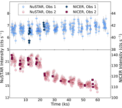
Figure 1: Light curve for the NuSTAR and NICER observations of SLX 1735$-$269 binned to 128 s. The top panel represents Obs 1 and the bottom represents Obs 2. Only one NuSTAR focal plane module (FPM) is shown for clarity.

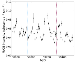
Figure 2: A long term MAXI light curve for the source. Vertical lines indicate the dates at which Obs 1 (left, blue) and Obs 2 (right, red) occur. We see that Obs 1 occurs during a lower flux state than Obs 2. The MAXI data are binned to 10 days.

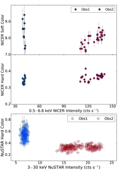
Figure 3: Color-Intensity diagrams for NICER and NuSTAR observations of SLX 1735$-$269. The top and middle panels represent the soft and hard color in NICER (respectively defined using the bands 1.1-2.0 keV/0.5-1.1 keV and 3.8-6.8 keV/2.0-3.8 keV), and the bottom panel represents the hardest color measurement in NuSTAR, defined using the bands 10-16 keV/6.4-10 keV

.

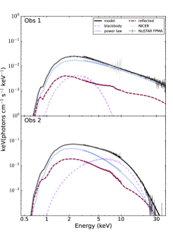
Figure 4: Shown here are the unfolded spectra and the respective model components from xillverCO for both observations. We can see here that Obs1 has an overall lower flux and different shape to that of Obs 2, which displays a cutoff in the power law around 5.5 keV.

3 Spectral Modeling and Timing Analysis

In this section we discuss the process used to model both the continuum and the reflected emission, as well as an analysis of some of the timing properties of this system.

3.1 Continuum modeling

We begin by modeling the spectrum of SLX 1735$-$269 with only a continuum description. This continuum is comprised of a blackbody of temperature, $kT_{\mathrm{bb}}$, representing the thermal emission from the NS, and a cutoff power law representing the illuminating corona with an index of $\Gamma_{\mathrm{pl}}$. We account for absorption of the continuum along the line of sight with tbabs with a hydrogen column density of $N_{H}$. With tbabs, we use the wilm abundance (Wilms et al., 2000) and vern cross-sections (Verner et al., 1996). We reconcile the calibration differences between NICER and NuSTAR using a model of the form $CE^{-\Delta\Gamma}$ (Steiner et al., 2010). We hold the constant $C$ to be 1 for the NuSTAR focal plane module A (FPMA) spectrum, and fix $\Delta\Gamma=0$ in both NuSTAR spectra. We allow the constant to vary in the NuSTAR FPMB and in NICER, and allow $\Delta\Gamma$ to vary in NICER to adjust for the difference in slope due to calibration differences.

With the model in place we fit the data for both observations using the xspec v12.13.1 (Arnaud, 1996). With a reasonable starting place, we then run a Markov Chain Monte Carlo (MCMC) fit in xspec with 100 walkers, a burn in of 100000 and a length of 10000. The results of that fit are listed in Table 2. We can see that notably the cutoff energy is much lower for Obs 2, indicating alongside Figure 3 that the system entered a much softer state. The high-energy cutoff expected for LMXB systems frequently moves to lower energies (Degenaar et al., 2018). This cutoff at lower energies is visible in the shape of the spectra for Obs 2, which can be seen in Figure 4. Obs 1 smoothly follows a single power law within the bounds of these spectra, and so the cutoff energy for this observation should not be considered a physical result.

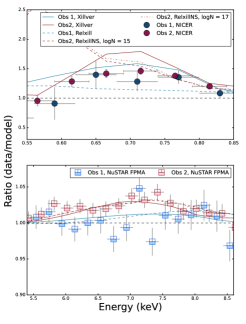
Figure 5: Shown here are the regions containing the (top) O VIII Ly$\alpha$ and (bottom) Fe K$\alpha$ reflection. These are constructed by ignoring the regions surrounding the line in xspec, fitting a continuum, then reintroducing these regions and plotting the ratio of the data to the model. We see strong evidence for a feature around the O VIII energy band, but a feature around the Fe K$\alpha$ energy band is significantly weaker, at only about 3-4% above continuum

. We show the different models used and find that only xillverCO effectively detects the feature in the lower energy bands

Table 2: Continuum

	Obs 1	Obs 2
CFPMB	$0.983\pm 0.001$	$1.001\pm 0.004$
CNICER	$0.85_{-0.08}^{+0.04}$	$0.89\pm 0.03$
$\Delta\Gamma$ (10-2)	$-7.0_{-6.7}^{+3.6}$	$-8.6_{-1.8}^{+2.4}$
$N_{\rm H}$ (1022 cm-2)	$1.62\pm 0.04$	$1.51\pm 0.02$
$kT_{\mathrm{bb}}$ (keV)	$0.69_{-0.06}^{+0.04}$	$2.01\pm 0.02$
kbb(10-3)	$0.34_{-0.07}^{+0.04}$	$3.0\pm 0.1$
$\Gamma_{\mathrm{pl}}$	$1.92_{-0.02}^{+0.07}$	$1.7\pm 0.1$
Ecut,pl (keV)	$125_{-41}^{+123}$	$5.9_{-0.3}^{+0.2}$
kpl	$0.072_{-0.003}^{+0.009}$	$0.25\pm 0.01$
$\chi^{2}$ (dof)	428(386)	676(356)

Note: All errors are reported at the 90% confidence interval. The blackbody normalization (k_bb) is defined as $(L/10^{39}$ erg s${}^{-1})/(D/10$ kpc)², and the powerlaw normalization (k_pl) is defined as photons keV^-1 cm^-2 s^-1 at 1 keV.

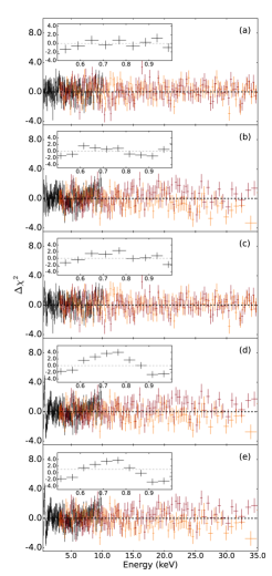
Figure 6: Shown above are the model residuals for the full X-ray band in NICER (black) and NuSTAR (Orange/Red for FPMA/FPMB respectively). The panels show the residuals for (a) Obs1 using xillverCO, (b) Obs2 using xillverCO, (c) Obs1 using relxill, (d) Obs2 using relxillNS with $\log N=15$, and (e) Obs2 using relxillNS with $\log N=17$. The insets display the NICER 0.5-1.0 keV energy range to highlight the difference in fit quality for the area in which we expect an O VIII Ly$\alpha$ for an UCXB.

We look for evidence of reflected features by inspecting regions surrounding the expected features. We initially ignore data bins between 0.6-0.8 keV (corresponding to the O VIII Ly$\alpha$ feature expected for CO WD UCXBs at around 0.67 keV) and 5.5-7.4 keV (corresponding to the Fe K$\alpha$ feature around 6.4 keV). We fit the continuum with these regions ignored, then reintroduce them and plot the ratio of the data to the model. The results of this plotting can be seen in Figure 5. We see that the feature around the energy band of Fe K$\alpha$ peaks at around 4%, quite a bit lower than the 10-15% seen in some canonical LMXBs (for example, Ser X-1, see Ludlam et al. 2018). However, a very strong feature (around 50% above continuum) is seen at the lowest energies. Figure 6 also shows that the non-UCXB models perform worse in the lower energy than xillverCO. Because Obs2 is background dominated above roughly 30 keV, the residuals are dominated by this regime, but we also note that relxillNS also under performs in this regime. However, all perform about equally well in energy ranges outside of these. It should be noted that these features can often be overestimated if other absorption effects such as absorption edges are not accounted for (Ludlam et al., 2020). In fact, we do see from Figure 5 that in Obs2, the contribution from xillverCO does not fully account for the reflection feature. However we find that edges included in the model are poorly constrained and do not significantly impact fit quality, so we exclude these from our model.

3.2 Reflection Modeling

With the continuum model in place, we then compare two different reflection models. The first is xillverCO convolved with relconv. xillverCO is a reflection table with carbon and oxygen abundances similar to what is seen in CO WDs. This reflection table is used to model the spectra of UCXBs and is based off of the existing xillver models in the relxill family of models (Madej et al., 2014; Ludlam et al., 2020). In this model, we allow the CO abundance (A_CO), the disk temperature at the region of reflection (kT_refl), the ratio of the incident flux to that of the emergent blackbody flux at the region of reflection, and the normalization to be free. We tie the E_cut in xillverCO to that of the cutoff powerlaw. We fix the redshift to 0 since the source is Galactic.

Table 3: Reflection Model Comparison

	Relxill	RelxillNS		XillverCO
	Obs 1	Obs 2		Obs 1	Obs 2
CFPMB	$0.98\pm 0.01$	$1.000_{-0.002}^{+0.006}$	$1.001_{-0.004}^{+0.006}$	$0.983_{-0.005}^{+0.002}$	$1.000_{-0.002}^{+0.006}$
CNICER	$0.87_{-0.02}^{+0.01}$	$0.85\pm 0.03$	$0.82_{-0.02}^{+0.05}$	$0.87_{-0.03}^{+0.05}$	$0.85_{-0.04}^{+0.02}$
$\Delta\Gamma$(10-2)	$-4.9_{-0.6}^{+0.4}$	$-11.2_{-2.5}^{+1.7}$	$-14.1_{-1.2}^{+3.9}$	$-5.1_{-2.5}^{+4.4}$	$-11.4_{-2.9}^{+1.5}$
$N_{\rm H}$ (1022 cm-2)	$1.78_{-0.05}^{+0.04}$	$1.37_{-0.03}^{+0.02}$	$1.25_{-0.02}^{+0.04}$	$1.67_{-0.03}^{+0.05}$	$1.66_{-0.02}^{+0.04}$
kTbb (keV)	$0.72_{-0.04}^{+0.03}$	$1.74_{-0.01}^{+0.20}$	$1.6_{-0.1}^{+0.2}$	$0.67\pm 0.03$	$2.05_{-0.01}^{+0.03}$
kbb(10-3)	$0.42\pm 0.03$	$3.1_{-0.5}^{+1.0}$	$3.6\pm 0.6$	$0.37_{-0.05}^{+0.03}$	$3.5_{-0.2}^{+0.1}$
$\Gamma_{\mathrm{pl}}$	$1.86_{-0.02}^{+0.01}$	$0.8\pm 0.1$	$0.05_{-0.05}^{+0.2}$	$1.93_{-0.03}^{+0.04}$	$1.69_{-0.024}^{+0.16}$
Ecut,pl	$95_{-13}^{+5}$	$1.6_{-0.1}^{+0.2}$	$1.01_{-0.01}^{+0.13}$	$145_{-36}^{+40}$	$5.0_{-0.2}^{+0.6}$
kpl	$0.017_{-0.001}^{+0.002}$	$0.31_{-0.02}^{+0.01}$	$0.37_{-0.06}^{+0.01}$	$0.07\pm 0.01$	$0.17_{-0.01}^{+0.07}$
q	$3.5_{-0.1}^{+0.2}$	$3.5_{-0.9}^{+1.2}$	$3.9_{-1.6}^{+3.0}$	$3.6_{-1.4}^{+0.9}$	$2.5_{-0.5}^{+2.5}$
$i$ (deg)	$72.8_{-2.3}^{+2.9}$	$55.8_{-2.5}^{+11.2}$	$47.6_{-12.4}^{+9.5}$	$59.4_{-3.1}^{+21.2}$	$54.9_{-4.7}^{+19.0}$
$R_{in}$ (RISCO)	$1^{\dagger}$	$1.7_{-0.6}^{+1.5}$	$1.3_{-0.3}^{+2.7}$	$1.4_{-0.4}^{+2.5}$	$1.7_{-0.6}^{+5.8}$
AFe/CO	$0.54_{-0.04}^{+0.08}$	$0.6_{-0.2}^{+0.7}$	$0.53_{-0.03}^{+0.64}$	$47_{-11}^{+40}$	$38_{-3}^{+16}$
kTrefl (10-2 keV)	—	$2.7_{-0.1}^{+0.2}$	$2.8\pm 0.2$	$8.7_{-2.1}^{+0.1}$	$9.6_{-0.8}^{+0.3}$
frac	$0.03\pm 0.01$	$10.1_{-15.1}^{+1.2}$	$8.6_{-12.9}^{+1.3}$	$0.11_{-0.02}^{+0.11}$	$0.10\pm 0.02$
krefl (10-410-9)	$3.8\pm 0.2$	$0.35_{-0.1}^{+0.4}$	$0.4_{-0.1}^{+0.4}$	$0.5_{-0.1}^{+0.5}$	$3.1_{-0.4}^{+1.2}$
$\log{N}({\mathrm{c}m}^{-3})$	—	15∗	17∗	—
$\log{\xi}$	$3.5\pm 0.1$	$3.4\pm 0.2$	$3.6\pm 0.3$	—
$\chi^{2}$ (dof)	398 (379)	467 (348)	429(348)	395(380)	415 (349)

Note: $\dagger=$ Errors returned are $\pm 0$, so we assume the chain is insensitive to this parameter, forcing it to one of the bounds. All errors are reported at the 90% confidence interval. For comparison some rows are used for both relxillNS and xillverCO despite having slightly different definitions in their respective models. A_CO/Fe refers to the carbon and oxygen abundance (A_CO) in xillverCO and the iron abundance (A_Fe) in relxillNS. The frac parameter represents different reflections as well. In xillverCO, frac represents the ratio of the illumianting powerlaw to that of the emergent blackbody from the disk (kT_refl), whereas frac in relxillNS represents the ratio of the illuminating X-rays to those that escape to infinity. The blackbody normalization (k_bb) is defined as $(L/10^{39}$ erg s${}^{-1})/(D/10$ kpc)², and the powerlaw normalization (k_pl) is defined as photons keV^-1 cm^-2 s^-1 at 1 keV.

Because xillverCO does not account for the relativistic broadening of reflected features, we must convolve the model with relconv, which can be used to determine certain physical parameters of the system. Specifically we can use it to determine the inner disk radius at which the reflection is occurring (R_in), which we report in terms of the innermost stable circular orbit ($R_{\mathrm{ISCO}}$), the orbit at which a test particle can orbit stably without falling onto the neutron star, 6 gravitational radii $R_{g}$ =12.4 km for a 1.4 M_⊙, non-rotating neutron star), assuming the reflection occurs at the innermost region of the disk. In this model we assume that for a NS only one emissivity index is necessary, so we fix both indices to be equal $q_{1}=q_{2}=q$ and fix the break radius to 500$R_{g}$. Since the X-rays only probe the innermost region of the disk, we fix the outer disk to 990 $R_{g}$. We tie the inclination measured from relconv to that measured with xillverCO. We also fix the limb parameter and the dimensionless spin to 0. We choose 0 following Ludlam et al. (2018), who shows that the effect of the spin is minimal for most LMXBs. The fitting process described in Section 3.1 is repeated, and the results are shown in the rightmost two columns of Table 3.

In order to compare the results of a model with UCXB abundances to those with more typical solar abundances, such as a NS LMXB, we then replace the relconv*xillverCO in observations 1 and 2 with relxillNS and relxill, respectively, to account for relativistic reflection. The difference between these models lies in the illuminating source– relxillNS assumes the disk is illuminated by a thermally dominated boundary layer, where relxill uses a coronal, non-thermal illuminating source. The different states between our two observations require that we treat each model accordingly when testing for a disk composed of solar abundance material. Many of the parameters remain the same between all three models, with a few exceptions. For one, the A_CO representing the carbon and oxygen abundance in xillverCO is replaced with the iron abundance, A_Fe in relxill/relxillNS. The frac parameter in Table 3 represents the ratio of illuminating flux to that which is reflected for relxill and relxillNS. relxill and relxillNS also have a few unique parameters. Both models have the parameter $\log\xi$ which represents the ionization of the disk ($\xi=L$, and relxillNS has the parameter $\log N$ which represents the density of the disk in cm^-3. To properly compare this model to the other models, we fix it both to 15 (the fixed value in relxill) and 17 (the fixed value in xillverCO) (García et al., 2022; Madej et al., 2014). The results of these models are found in Table 3.

Because the feature around O VIII is heavily binned and the feature surrounding Fe K$\alpha$ is weak, we attempt to test the confidence of these measurements. We first apply a Gaussian to the continuum model with its center fixed at 0.67 keV and detect the feature with $>3.5\sigma$ and $>8.5\sigma$ significance using an f-test in Obs 1 and 2, respectively. We then repeat the process, but at 6.4 keV and detect a feature near iron with $>4.5\sigma$ and $>8.5\sigma$ significance in Obs 1 and 2 respectively. We also test the significance of the spectral broadening by fitting the data with and without relconv. We find that including relconv to the model has only $\sim 1.6\sigma$ significance for Obs1 but $>5\sigma$ for Obs 2, likely due to the increased flux in Obs 2. This indicates that the broad features are in fact associated with the reflected emission and do not arise from elsewhere in the system.

3.3 Timing Analysis

Since the key defining parameter of a UCXB is a period of $<$ 80 minutes, we attempt to search for evidence of periodicity in the X-ray light curves. Wijnands & van der Klis (1999) suggests that the inclination angle of the source may be quite high, leading to a smearing of pulsations. A high inclination should result in eclipses in the X-ray light curve, yet none are seen in the data, which is supported by in’t Zand et al. (2007). In order to search for a periodicity in the X-ray light curves, we construct a Lomb-Scargle periodogram using the scipy.signal Python module (Lomb, 1976; Scargle, 1982). We do so using both observations individually as well as combined. We detrend both observations by conducting linear fits then dividing the data by the corresponding value. Obs 1 was fit with one line and Obs 2 was fit with 2 lines, breaking at a time of approximately 20 ks, as we can see in figure 1. However, no periodic frequencies aside from the length of time between GTIs are found. We therefore can not claim to have measured the period of the system.

4 Discussion and Conclusions

Between the two observations of SLX 1735$-$269, we find that the spectral shape changes significantly from a powerlaw dominated continuum to one dominated by thermal emission with a lower energy cut off. We find in Section 3 that the best fit statistics are achieved using xillverCO. Aside from the best fit statistics, the values retrieved from the fit are also generally more consistent with what we expect from a UCXB. Many of the reported parameters from relxillNS in Table 3 are unrealistic. For example in Obs 2, the power law index is lower than 1 (significantly so for the trial with $\log N$ fixed to 17), which is lower than the extreme hard spectral state for NSs (Ludlam et al., 2016; Parikh et al., 2017). A_Fe in all trials with relxill and relxillNS is also consistent with the lower bound of the model at 0.5. While this should not be taken as direct support that SLX 1735$-$269 is in fact a UCXB, this demonstrates that models with higher carbon and oxygen abundances do in fact provide a better explanation for the properties of the X-ray spectrum.

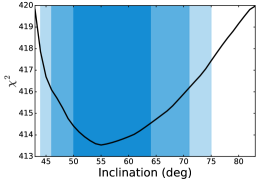
Figure 7: We use the steppar command in xspec to determine the sensitivity and quality of fit for the inclination measurement. We find that an inclination of around 55^∘ is a global minimum, though there is a slightly stronger bias against low inclinations than higher ones. Shown here are the results of steppar for Obs 2.The shaded regions represent the 68%, 90%, and 95% confidence intervals.

It should be noted that the count rates of these spectra are relatively low, especially so for Obs 1, which could affect the quality of the reflection features. Because of this, certain parameters that may be of key interest, such as $R_{\rm in}$, may not have the most reliable measurements. The $R_{\rm in}$ measurements listed in the xillverCO portion of Table 3 indicate that we observe some minor disk truncation during the higher flux state. We generally expect the disk to move inward at higher luminosities, but magnetic fields can complicate this by truncating accretion disks even at higher luminosities (Cackett et al., 2009; Ludlam et al., 2020). It should be noted however that the existence of a feature surrounding the O VIII Ly$\alpha$ energy range and none surrounding Fe K$\alpha$ prior to any modeling of reflection provides some evidence for non-solar carbon and oxygen abundances. This is also noted by Koliopanos et al. (2021), who finds that screening by the C and O abundances leads to a diminished Fe K$\alpha$ feature in the UCXB sources 4U 1543$-$624 and Swift J1756.9$-$2508.

We also present in this paper the first tentative measurement of the inclination of SLX 1735$-$269 at approximately $57^{+23}_{-6}$ degrees by taking the mean of the xillverCO measurements. As mentioned above, we do not expect an especially high inclination as we do not observe eclipsing in the light curve. We test whether this parameter is a significant contributor to the statistics in the fit using the steppar command in xspec, which varies just one parameter and measures the change in $\chi^{2}$. We find that there is some degree of sensitivity, with the $\chi^{2}$ value increasing by approximately 1 at 5 degrees on either side of the measured value, as shown in Figure 7.

After comparing multiple models and attempting various types of analysis we suggest the following:

1. xillverCO appears to provide a better fit for the X-ray spectra of SLX 1735$-$269 than relxill or relxillNS, which indicates that the carbon and oxygen abundance deviates from solar. This, alongside the evidence for a lower-energy oxygen feature, suggests that the source is more likely to be a UCXB than a canonical LMXB, strengthening the classification as a UCXB candidate. This is further supported by the fact the only xillverCO was able to model the feature in the low energy band. Relativistic broadening is statistically required to model these features, indicating they are in fact coming from reflection off of the rotating disk.

2. The reflection modeling using xillverCO has provided a tentative measurement of the inclination of this system at $57^{+23}_{-6}$ degrees. The reflection features used to measure both $R_{\rm in}$ and inclination are not very prominent, so further observations with longer exposures are needed to confirm.

3. Our timing analysis is inconclusive. The fact that no eclipses are present in the light curve is consistent with an inclination $\lesssim 80^{\mathrm{o}}$. A Lomb-Scargle periodogram does not reveal any measurable periodicity in the X-ray light curve. This means we can not conclusively deem the source to be a UCXB by any timing periodicities.

This study provides some additional indirect evidence in support of SLX 1735$-$269 being a UCXB candidate. We also present an early measurement of the inclination. Future studies using longer exposures in the soft X-rays (for example, from NICER) will be necessary to measure the orbital period and determine whether the source is ultra-compact in nature. Recent missions like XRISM could be useful in resolving reflection features, especially for testing for the existence of the faint Fe K$\alpha$ in these ultra-compact systems (Gandhi et al., 2022).

Acknowledgements: This research has made use of MAXI data provided by RIKEN, JAXA and the MAXI team (Matsuoka et al., 2009). This research has made use of data and/or software provided by the High Energy Astrophysics Science Archive Research Center (HEASARC), which is a service of the Astrophysics Science Division at NASA/GSFC. This research has made use of the NuSTAR Data Analysis Software (NuSTARDAS) jointly developed by the ASI Science Data Center (ASDC, Italy) and the California Institute of Technology (USA).

References

- Arnaud (1996) Arnaud, K. A. 1996, in Astronomical Society of the Pacific Conference Series, Vol. 101, Astronomical Data Analysis Software and Systems V, ed. G. H. Jacoby & J. Barnes, 17
- Bahramian & Degenaar (2023) Bahramian, A. & Degenaar, N. 2023, Handbook of X-ray and Gamma-ray Astrophysics. Edited by Cosimo Bambi and Andrea Santangelo, 120. doi:10.1007/978-981-16-4544-0_94-1
- Bazzano et al. (1997) Bazzano, A., Cocchi, M., Ubertini, P., et al. 1997, IAU Circ., 6668
- Cackett et al. (2008) Cackett, E. M., Miller, J. M., Bhattacharyya, S., et al. 2008, ApJ, 674, 415. doi:10.1086/524936
- Cackett et al. (2009) Cackett, E. M., Altamirano, D., Patruno, A., et al. 2009, ApJ, 694, L21. doi:10.1088/0004-637X/694/1/L21
- Chen et al. (2020) Chen, W.-C., Liu, D.-D., & Wang, B. 2020, ApJ, 900, L8. doi:10.3847/2041-8213/abae66
- Dauser et al. (2016) Dauser, T., García, J., Walton, D. J., et al. 2016, A&A, 590, A76. doi:10.1051/0004-6361/201628135
- Degenaar et al. (2018) Degenaar, N., Ballantyne, D. R., Belloni, T., et al. 2018, Space Sci. Rev., 214, 15. doi:10.1007/s11214-017-0448-3
- Fabian et al. (1989) Fabian, A. C., Rees, M. J., Stella, L., et al. 1989, MNRAS, 238, 729. doi:10.1093/mnras/238.3.729
- Fabian et al. (2012) Fabian, A. C., Wilkins, D. R., Miller, J. M., et al. 2012, MNRAS, 424, 217. doi:10.1111/j.1365-2966.2012.21185.x
- García et al. (2014) García, J., Dauser, T., Lohfink, A., et al. 2014, ApJ, 782, 76. doi:10.1088/0004-637X/782/2/76
- García et al. (2022) García, J. A., Dauser, T., Ludlam, R., et al. 2022, ApJ, 926, 13. doi:10.3847/1538-4357/ac3cb7
- Gandhi et al. (2022) Gandhi, P., Kawamuro, T., Díaz Trigo, M., et al. 2022, Nature Astronomy, 6, 1364. doi:10.1038/s41550-022-01857-y
- in’t Zand et al. (2007) in’t Zand, J. J. M., Jonker, P. G., & Markwardt, C. B. 2007, A&A, 465, 953. doi:10.1051/0004-6361:20066678
- Kaastra & Bleeker (2016) Kaastra, J. S. & Bleeker, J. A. M. 2016, A&A, 587, A151. doi:10.1051/0004-6361/201527395
- Koliopanos et al. (2014) Koliopanos, F., Gilfanov, M., Bildsten, L., et al. 2014, The X-ray Universe 2014, 102. doi:10.48550/arXiv.1404.0617
- Koliopanos et al. (2021) Koliopanos, F., Vasilopoulos, G., Guillot, S., et al. 2021, MNRAS, 500, 5603. doi:10.1093/mnras/staa3490
- Lomb (1976) Lomb, N. R. 1976, Ap&SS, 39, 447. doi:10.1007/BF00648343
- Ludlam et al. (2016) Ludlam, R. M., Miller, J. M., Cackett, E. M., et al. 2016, ApJ, 824, 37
- Ludlam et al. (2017) Ludlam, R. M., Miller, J. M., Bachetti, M., et al. 2017, ApJ, 836, 140
- Ludlam et al. (2018) Ludlam, R. M., Miller, J. M., Arzoumanian, Z., et al. 2018, ApJ, 858, L5. doi:10.3847/2041-8213/aabee6
- Ludlam et al. (2020) Ludlam, R. M., Cackett, E. M., García, J. A., et al. 2020, ApJ, 895, 45
- Madej et al. (2014) Madej, O. K., García, J., Jonker, P. G., et al. 2014, MNRAS, 442, 1157
- Matsuoka et al. (2009) Matsuoka, M., Kawasaki, K., Ueno, S., et al. 2009, PASJ, 61, 999. doi:10.1093/pasj/61.5.999
- Moutard et al. (2023) Moutard, D. L., Ludlam, R. M., García, J. A., et al. 2023, ApJ, 957, 27. doi:10.3847/1538-4357/acf4f3
- Miller et al. (2013) Miller, J. M., Parker, M. L., Fuerst, F., et al. 2013, ApJL, 779, L2
- Nelson et al. (1986) Nelson, L. A., Rappaport, S. A., & Joss, P. C. 1986, ApJ, 304, 231
- Parikh et al. (2017) Parikh, A. S., Wijnands, R., Degenaar, N., et al. 2017, MNRAS, 466, 4074. doi:10.1093/mnras/stw3388
- Savonije et al. (1986) Savonije, G. J., de Kool, M., & van den Heuvel, E. P. J. 1986, A&A, 155, 51
- Scargle (1982) Scargle, J. D. 1982, ApJ, 263, 835. doi:10.1086/160554
- Skinner et al. (1987) Skinner, G. K., Willmore, A. P., Eyles C. J., et al. 1987, Nature, 330, 544. doi:10.1038/330544a0
- Steiner et al. (2010) Steiner, J. F., McClintock, J. E., Remillard, R. A., et al. 2010, ApJ, 718, L117. doi:10.1088/2041-8205/718/2/L117
- Syunyaev et al. (1991) Syunyaev, R. A., Arefev, V. A., Borozdin, K. N., et al. 1991, Soviet Astronomy Letters, 17, 409
- Verner et al. (1996) Verner, D. A., Ferland, G. J., Korista, K. T., et al. 1996, ApJ, 465, 487. doi:10.1086/177435
- Wijnands & van der Klis (1999) Wijnands, R. & van der Klis, M. 1999, A&A, 345, L35. doi:10.48550/arXiv.astro-ph/9903450
- Wilkins & Fabian (2011) Wilkins, D. R. & Fabian, A. C. 2011, MNRAS, 414, 1269. doi:10.1111/j.1365-2966.2011.18458.x
- Wilkins (2018) Wilkins, D. R. 2018, MNRAS, 475, 748. doi:10.1093/mnras/stx3167
- Wilms et al. (2000) Wilms, J., Allen, A., & McCray, R. 2000, ApJ, 542, 914
- Wilson et al. (2003) Wilson, C. A., Patel, S. K., Kouveliotou, C., et al. 2003, ApJ, 596, 1220. doi:10.1086/377473