A Unified Approach to Second and Third Degree Price Discrimination

Abstract

We analyze the welfare impact of a monopolist able to segment a multiproduct market and offer differentiated price menus within each segment. We characterize a family of extremal distributions such that all achievable welfare outcomes can be reached by selecting segments from within these distributions. This family of distributions arises as the solution to the consumer maximizing distribution of values for multigood markets. With these results, we analyze the effect of segmentation on consumer surplus and prices in both interior and extremal markets, including conditions under which there exists a segmentation benefiting all consumers. Finally, we present an efficient algorithm for computing segmentations.

JEL Classification: D42, D83, L12

Keywords: Price Discrimination, Nonlinear Pricing, Private Information

1 Introduction

1.1 Motivation and Main Results

The welfare implications of a seller’s decision to price discriminate is a classic but important problem in economics. It has long been known that third degree price discrimination—the practice of charging different prices to consumers with different demands—may increase or decrease consumer surplus. The same holds for second degree price discrimination, in which sellers offer menus of products with varying quality or quantity.

Bergemann et al. (2015) show that with a monopoly seller of a single good, segmentation can achieve every possible division of surplus between the seller and consumers such that (1) consumer surplus plus profit does not exceed total available social surplus, (2) the seller receives at least the same profit as they would without segmentation, and (3) consumer surplus is nonnegative. The Pareto distribution with shape parameter 1 is critical to this result. In particular, they show that segmentations supported only on Pareto distributions can achieve every corner of the “surplus triangle,” and hence the interior of the entire triangle as well. Haghpanah and Siegel (2022) show that, in this setting, the full surplus triangle cannot be achieved when the seller can offer multiple goods at different costs. This paper extends the model of Bergemann et al. (2015) to incorporate second degree price discrimination.

We consider a multiproduct monopolist that can offer goods that are identical to the consumers but have different production costs. Consumers have multi-unit linear demands and their marginal utility (their valuation) is private information. The seller’s optimal strategy consist of posting a price for each good. The model is mathematically isomorphic to one in which the seller offers goods of varying quality that have different production costs: it suffices to consider each quality increment as a distinct good, and the marginal cost of each quality increment is the cost of each distinct good.

The critical distributions that are proved to be extremal in Bergemann et al. (2015) maintain the seller’s profits constant for every price in the support of possible values. With multiple goods with varying production cost, it is imposible to maintain the profits generate by each good constant for every price in the support of possible values. We instead introduce a natural extension, which consist of piecewise-defined generalized Pareto distributions. These distributions maintain the profits generated by each good constant for some values in the support, and each value in the support is an optimal price for some goods (Proposition 3 and Corollary 1). These distributions satisfy a crucial property that we repeatedly use in our analysis: among all distributions that keep the seller’s optimal prices fixed at a given level, the piecewise Pareto first-order stochastically dominates all other distributions (Theorem 1). For this same reason, it is straightforward to check that this family of distributions also allows characterizing the multigood version of the consumer-optimal distribution of values studied in Condorelli and Szentes (2020) (Proposition 4).

The piecewise Pareto distribution are also sufficient to characterize all achievable welfare outcomes (Theorem 2)—these are the extremal markets. By characterizing the extremal markets, we are able to analyze how segmentations affect prices and welfare, as well as more easily compute the entire space of achievable surplus divisions. We show that market segmentations of extremal and interior markets are contrastingly different (Proposition 6 and 8). We thus have that the piecewise Pareto distributions generalize the unit-elasticity demand function that plays a crucial role in Bergemann et al. (2015) and in Condorelli and Szentes (2020).

The organization of this paper is as follows. Section 2 introduces our model of nonlinear pricing with market segmentation. In section 3, we provide the single-good benchmark for our results. While doing so, we also introduce the consumer maximization problem, and demonstrate its connection with market segmentations. Section 4 defines the piecewise generalized Pareto distributions which we work with for the remainder of the paper. We show that these distributions both solve the multigood consumer maximization problem, and use them to characterize extremal markets. Using these results, section 5 analyzes how segmentation can improve consumer welfare and lower prices, in both interior and extremal markets. Finally, section 6 discusses our results in the context of the surplus polytope, a visual representation of the welfare effects of price discrimination. Appendix A considers an extension to continuous types and qualities. We are able to characterize the solution to the consumer maximization problem using an optimal control program, and conjecture a relationship between this family of distributions and the welfare outcomes of segmentation. Proofs omitted from the main text can be found in Appendix B.

1.2 Related Literature

Our results are related to a large literature on price discrimination, beginning with Pigou (1920) and now encompassing a wide range of research on the output and welfare implications of price discrimination, such as Robinson (1969); Schmalensee (1981); Varian (1985); Aguirre et al. (2010); Cowan (2016). We use the classic model of second-degree price discrimination via quality and quantity differentiated products first presented by Mussa and Rosen (1978) and Maskin and Riley (1983). Of particular relevance is the work of Johnson and Myatt (2003), who consider a model of a producer combining second and third degree price discrimination. The family of distributions which underpins our main results arises from solving a multigood version of the consumer maximization problem considered by Condorelli and Szentes (2020), which is also closely related to the problem studied by Roesler and Szentes (2017).

The problem of extending the results of Bergemann et al. (2015) to a multigood setting is also studied by Haghpanah and Siegel (2022) and Haghpanah and Siegel (2023). Haghpanah and Siegel (2022) show that in multigood settings, the full surplus triangle is not achievable. Both of these papers consider models that are more general than ours as, among other things, they allow for some horizontal differentiation among consumers. Haghpanah and Siegel (2022) characterize when the full triangle of feasible surplus pairs can be achieved; in our model, the full surplus triangle cannot be achieved. We provide complementary conditions on when the full triangle cannot be attained. In Haghpanah and Siegel (2023), the authors construct a Pareto-improving binary segmentation for generic markets. Our main contribution relative to Haghpanah and Siegel (2023) is that we provide a characterization of extremal markets, which turn out to be non-generic extremal markets for which their argument fails to hold. By doing so, we are able to provide an alternate proof that Pareto improvements are possible when the aggregate market is interior, while in extremal markets, no segmentation makes all consumers better off. Despite this, we show that in extremal markets, segmentation can still increase aggregate consumer surplus. Our characterization of extremal markets allows to more easily compute the surplus pairs that are attainable via market segmentation and characterize the consumer-optimal distribution of values.

2 Setup

There is a monopolist and a continuum of consumers. Each consumer has a type, drawn from the set $V=\{v_{1},\dots,v_{k},\dots,v_{K}\}\subset\mathbb{R}_{+}$. Consumers value each good at their type $v$, and each consumer knows their type. A market $x$ is a distribution over $V$. We denote the demand in market $x$ by:

$$D_{x}(v)\triangleq\sum_{v_{k}\geq v}x(v_{k}).$$

Since there is a bijection between a market and its demand, we frequently, in an abuse of notation, identify a market with its demand function.

The monopolist sells $n$ goods, with the cost of producing good $i$ being $c_{i}\geq 0$. We order the goods so that $c_{i}$ is strictly increasing and $c_{n}<v_{K}$, so it is socially efficient to supply every good to the buyer with the highest valuation. The monopolist posts a menu of prices $p=\{p_{i}\}_{i\in n}$. For each $i$, the consumer buys good $i$ if and only if their type $v\geq p_{i}$. Good $i$ generates profits:

$$\Pi_{i}(x,p)\triangleq D_{x}(p_{i})(p_{i}-c_{i}).$$

We sometimes write the profits as $\Pi_{i}(x,p_{i})$ since they only depend on the $i$-th component of the price vector. The price vector $p$ generates aggregate profits:

$$\Pi(x,p)\triangleq\sum_{i\in n}\Pi_{i}(x,p).$$

We say that a price vector $p$ is optimal if there is no other price vector which yields a higher profit, and use $p^{x}$ to denote optimal prices for market $x$. Since a market may have multiple optimal prices, we use $\underline{p}^{x}$ and $\overline{p}^{x}$ to denote the lowest and highest optimal prices, respectively.

In a similar vein, the consumer surplus generated by selling good $i$ at a price of $p_{i}$ is:

$$U_{i}(x,p)\triangleq\sum_{v_{k}\geq p_{i}}x(v_{k})(v_{k}-p_{i}).$$

The aggregate consumer surplus in market $x$ when prices are $p$ is then:

$$U(x,p)\triangleq\sum_{i\in n}U_{i}(x,p).$$

Note that we can also interpret this setup as a model of second degree price discrimination à la Mussa and Rosen (1978) or Maskin and Riley (1983), where the goods are increments of quality or quantity, and $p_{i}$ is the marginal price. Under this interpretation, the consumer selects a quality or quantity $q\in\{0,\dots,n\}$, receives utility $vq$, and pays price $\sum_{i\leq q}p_{i}$.

2.1 Market Segmentation

The goal of this paper is to understand how profits and consumer surplus vary when the seller is able to divide consumers into different submarkets, and price optimally within each one. That is, the seller is able to engage in both second and third degree price discrimination simultaneously. Segments may be arbitrarily constructed, subject to the constraint that they aggregate together to the original market.

Let $x^{\ast}\in\Delta V$ denote the aggregate market, $p^{\ast}$ the optimal prices in the aggregate market, and $\Pi^{\ast}=\Pi(x^{\ast},p^{\ast})$ the resulting profit. We will refer to $\Pi^{\ast}$ as the aggregate monopoly profit.

Definition 1 (Segmentation)

A segmentation of $x^{\ast}$ is a distribution $\sigma$ over $\Delta V$ such that $\sum_{x\in\Delta V}\sigma(x)x=x^{\ast}$.

Given a price vector $p$, we can consider the (possibly empty) set of markets where $p$ is optimal:

$$X_{p}\triangleq\left\{x\in\Delta V\mid\Pi(x,p)\geq\Pi(x,p^{\prime})\ \forall p^{\prime}\right\}.$$ (1)

This is a compact, convex subset of $\mathbb{R}_{+}^{n}$, so by the Krein-Milman Theorem, it is equal to the convex hull of its extreme points, which we call extremal markets.

Figure 1 represents the simplex $\Delta V$ when there are three values and two goods. The different regions $X_{p}$ are identified by a vector that identifies the optimal prices in each region. As long as the most expensive good is cheaper than the smallest value, the simplex and the different regions will look qualitatively the same. We do not require this assumption for our analytical results, but we will come back to this illustration when we do specific examples.

The extreme points of $X_{p}$, which are the focus on this paper, are the intersections of the different lines. We refer to these as extremal markets. In Figure 1 there are three interior extremal markets, illustrated with a white, red and blue dots. The white dot is a market in which the seller is indifferent between the three prices $p\in\{1,2,3\}$ for good 1 (the cheaper good) and the optimal price for the second (more costly to produce) good is $p=3.$ The blue dot is a market in which the seller is indifferent between the three prices $p\in\{1,2,3\}$ for good 2 and the optimal price for the first (cheaper) good is $p=1.$ The red dot is a market such that the seller is indifferent between the prices $p\in\{1,2\}$ for the first good and is indifferent between the prices $p\in\{2,3\}$ for the second good. There are other extremal markets in which the support of the distribution is smaller. The extremal markets marked by gray dots illustrate points in which the buyer has a valuation of 3 with probability of 1 and another one in which the buyer never has a valuation of 2 but the seller is indifferent between the prices $p\in\{2,3\}$ for the second good.

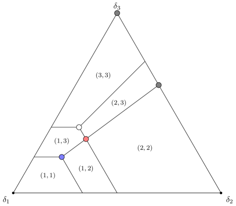
Figure 1: Division of $\Delta V$ into $X_{p}$ when there are three values ($V=\{1,2,3\}$), and two goods ($n=2$ with $c=(0,\frac{1}{3})$).

Definition 2 (Extremal segmentation)

A segmentation $\sigma$ of $x^{\ast}$ is extremal if every market $x\in\operatorname{supp}(\sigma)$ is an extreme point of $X_{p^{x}}$.

In general, we may know very little about the segments $x$. However, by definition, $x\in X_{p^{x}}$, meaning we can replace each $x$ with a convex combination of extreme points of $X_{p^{x}}$ while keeping prices the same. The resulting segmentation is extremal, with the same consumer surplus and profit as before. Thus, the extreme points of $X_{p}$ are sufficient to capture the welfare implications of segmentation. The main result of this paper is to characterize these extreme points.

3 Single-Good Benchmark

It turns out that finding the extreme points of $X_{p}$ is related to the problem of the finding the consumer-optimal distribution of values across all possible distributions, which we call the consumer maximization problem. In this section, we define the consumer maximization problem, and demonstrate its connection to the characterization of extremal markets by presenting the single-good benchmark for both (that is, $n=1$). In doing so, we hope to highlight the main elements of the analysis which will be useful for our results.

3.1 Consumer Maximization Problem

It is easy to see that, in general, increasing the distribution of values will increase profits. In fact, both 0 and $v_{K}$ (the maximal valuation) are the profits when the distribution of values is degenerate at 0 or $v_{K}$, respectively. Everything in between is achievable with an intermediate distribution.

However, when we examine how the distribution of values impacts consumer surplus, the effect is more subtle. In particular, if the distribution of values is degenerate, the seller can extract the full surplus. Hence, the problem of finding the distribution of values which maximizes consumer surplus is not trivial. Formally, we wish to solve:

$$\max_{\begin{subarray}{c}x\in\Delta V\\ p\in V\end{subarray}}\Big{[}U(x,p)\Big{]}\text{ such that }p\in\operatorname*{arg\,max}_{\hat{p}\in V}\Big{[}\Pi(x,\hat{p})\Big{]}.$$ (2)

Note that in this problem the price is a scalar because we are focusing on the problem when there is just 1 good.

We begin with the solution to (2) when $n=1$. This problem is analyzed by Condorelli and Szentes (2020) when there is a continuum of values and $c=0$. Condorelli and Szentes (2020) show that, for $n=1$, the consumer-optimal distribution of values is

$$F^{\ast}(v)=\begin{cases}1-\frac{1}{ev}&\frac{1}{e}\leq v<1\\ 1&v\geq 1\end{cases},$$

which is the Pareto distribution with shape 1 and scale $\frac{1}{e}$ truncated on the interval $[\frac{1}{e},1]$.

The assumption of continuous values, compared with our discrete setting, does not change the nature of the result. Additionally, when $n=1$, assuming the cost is 0 is without loss of generality. However, for $n\geq 2$, we can no longer normalize all costs to 0, so it is convenient to “undo” the normalization even for the one good benchmark.

Proposition 1 (Consumer-optimal distribution ($n=1$))

Let $(x,p)$ be a solution to (2), then $x$ satisfies:

$$D_{x}(v_{k})=\frac{p-c}{v_{k}-c}\text{ if }v_{k}\geq p,$$ (3)

and $D_{x}(v_{k})=1$ if $v_{k}<p$.

The distribution is constructed as to keep profits constant for every price in $[p,v_{K}]$, and (given this indifference) the seller sells the good at the lowest optimal price. Indeed, when the demand is given by (3), we have:

$$\Pi(x,v_{k})=p-c,$$

for all $v_{k}\geq p$. We thus have that the seller is indifferent between all these prices.

3.2 Extremal Segmentations

Bergemann et al. (2015) characterize the extreme points of $X_{p}$ when $n=1$. We see that there is a connection between these extreme points and the distribution given by (3).

Proposition 2 (Extreme points of $X_{p}$ ($n=1$))

When $n=1$, if $x$ is an extreme point of $X_{p}$, then for some $S\subseteq V$:

$$D_{x}(v_{k})=\begin{cases}\frac{A}{v_{k}-c}&\text{if }v_{k}\in S\\ D_{x}(v_{k+1})&\text{otherwise}\end{cases},$$

where $A=\min\{S\}-c$ is the profit from selling at a price equal to the lowest value in $S$.

In this case, we have that the extreme points of $X_{p}$ may place positive mass in only a subset of values in $V$, which are denoted by $S\subset V$. Once again, if the price is equal to any $v_{k}\in S$, we have that profits remain constant:

$$\Pi(x,v_{k})=A=\min\{S\}-c$$

Prices not in $S$ are never optimal.

4 Piecewise Pareto Distributions

We now return to the multigood setting with general cost vectors $c\geq 0$. First, we define a family of distributions, and present a few of its key properties. We then show that the consumer-optimal distribution of values in the multigood setting is in this family of distributions. In the next section we will show that extremal markets are also in this family of distributions.

4.1 Piecewise Generalized Pareto Distributions

With a single good, the relevant distributions keep the seller’s profits constant. Of course, with multiple goods, it is impossible to construct a demand function that keeps profits constants for every good simultaneously; instead, the demand function will maintain constant profit for some good in different intervals of consumer types.

Let $r=\{r_{i}\}_{i\in n}\in V^{n}$ be an increasing sequence such that $c_{i}<r_{i}$ and denote $r_{i+1}=v_{K}$. These will be the cutoffs that determine the different segments. We then define:

$$D_{r}(v_{k})\triangleq\frac{A_{i}}{v_{k}-c_{i}}\text{ if }v_{k}\in(r_{i},r_{i+1}]$$ (4)

and $D_{r}(v_{k})=1$ for all $v_{k}\leq r_{1}$. The constants $\{A_{i}\}_{i\in n}$ are defined as follows: $A_{1}\triangleq r_{1}-c_{1}$, and for every $i\geq 2$:

$$A_{i+1}\triangleq A_{i}\frac{r_{i+1}-c_{i+1}}{r_{i+1}-c_{i}}.$$ (5)

We illustrate a few examples of demand functions which satisfy (4) in Figure 2. We plot in the limit as $V$ becomes the interval $[0,1]$ as it will help gain additional intuition for the construction.

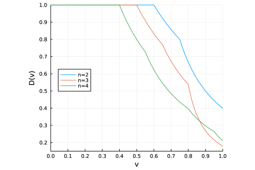
Figure 2: Demands satisfying (4)

In Figure 3 we plot the profit from selling each good $i\in\{1,\dots,4\}$ at various prices when demand is the one in Figure 2 (in the case $n=4$). We can see that for each good there are multiple optimal prices and every price in the domain of values is the optimal price of some good. The values at the kinks $(0.55,0.8,0.95)$ are optimal prices for two goods simultaneously. Indeed, the constants $\{A_{i}\}$ will be constructed such that the values at the cutoffs $r$ are an optimal price for two goods simultaneously (except for the first cutoff). We now formalize these graphical intuitions. That is, we now show that under this demand function, the profit generated by selling good $i$ at price $v_{k}$ is increasing below $r_{i}$, constant in the interval $[r_{i},r_{i+1}]$, and decreasing above $r_{i+1}$.

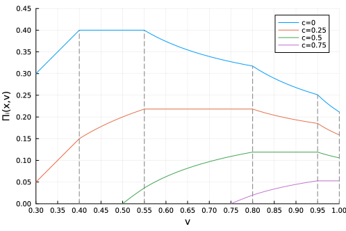
Figure 3: Profits under $D_{r}$

Proposition 3 (Profit under $D_{r}$)

For every $v_{k}\in[r_{i},r_{i+1})$, we have: (a) $\Pi_{i}(D_{r},v_{k})=\Pi_{i}(D_{r},v_{k+1})$; (b) If $c_{j}>c_{i}$, $\Pi_{j}(D_{r},v_{k})<\Pi_{j}(D_{r},v_{k+1})$; (c) If $c_{j}<c_{i}$, $\Pi_{j}(D_{r},v_{k})>\Pi_{j}(D_{r},v_{k+1})$.

Proof.

By definition, for $v_{k}\in(r_{i},r_{i+1}]$, we have:

$$\Pi_{i}(D_{r},v_{k})=D_{r}(v_{k})(v_{k}-c_{i})=A_{i}.$$

We thus immediately have that part (a) is satisfied for all $v_{k}\in(r_{i},r_{i+1})$. We only need to verify it is also satisfied for $v_{k}=r_{i}.$ In this case, we have that:

$$\Pi_{i}(D_{r},v_{k-1})=\frac{A_{i-1}}{r_{i}-c_{i-1}}(r_{i}-c_{i})=A_{i}.$$

This establishes (a). Parts (b) and (c) follow from observing that if decreasing the price keeps profits constant when the cost is $c_{i}$, the profits will strictly decrease when the cost is larger than $c_{i}$ and strictly increase when the cost is smaller than $c_{i}$.    

We can then also explicitly state that every value in the support of values is an optimal price for some good.

Corollary 1 (Optimal prices under $D_{r}$)

Every price in $[r_{i},r_{i+1}]$ is an optimal price for good $i$.

Another useful implication of Proposition 3 is to identify when prices can be optimal for some market, that is, when the set $X_{p}$ is non-empty.

Corollary 2 (Non-empty $X_{p}$)

The set of markets under which price $p$ is optimal $X_{p}$ is non-empty if and only if for all $i\in\{1,..,n\}$, (a) $p_{i}\leq p_{i+1}$ and (b) $c_{i}<p_{i}$.

Proof.

For any prices satisfying the conditions in this corollary, $D_{p}\in X_{p}$ and so $X_{p}$ is non-empty. To prove the conditions are also necessary, we note that $p_{i}<c_{i}$ is obviously never optimal. We can also easily verify that when $c_{i}<c_{i+1}$, for any two prices $p<\hat{p}$ and any market $x$:

$$D_{x}(\hat{p})(\hat{p}-c_{i})-D_{x}(p)(p-c_{i})<D_{x}(\hat{p})(\hat{p}-c_{i+1})-D_{x}(p)(p-c_{i+1}).$$

Hence, $p_{i}>p_{i+1}$ is not optimal.    

Later, we will use (4) to characterize the extreme points of $X_{p}$. Corollary 2 assures us that the restrictions on $r$ in our construction of $D_{r}$ are without loss.

4.2 Multigood Consumer Maximization Problem

The consumer-optimal distribution of values in the multigood case follows from the next result:

Theorem 1 (Stochastic dominance)

The distribution $x\in\Delta V$ is first-order stochastically dominated by any $D_{r}$ when $r_{i}\geq\underline{p}^{x}_{i}$ for all $i$.

Proof.

To make the notation more compact, throughout the proof we denote shortly $p_{i}=\underline{p}_{i}^{x}$. We claim that given any two price vectors $p,\hat{p}$ with $p_{i}\leq\hat{p}_{i}$ for all $i$, $D_{\hat{p}}$ first-order stochastically dominates any $x\in X_{p}$. That is, for all $v_{k}\in V$, $D_{x}(v_{k})\leq D_{\hat{p}}(v_{k}).$ Suppose, by contradiction, there exists $\hat{v}$ such that $D_{x}(\hat{v})>D_{\hat{p}}(\hat{v})$, and without loss assume $\hat{v}$ is the smallest such value. Let $p_{i}$ be such that $\hat{v}\in(p_{i},p_{i+1}]$. Note that $\hat{v}>\hat{p}_{1}\geq p_{1}$, so such $p_{i}$ exists. We then have that:

$$\Pi_{i}(D_{x},\hat{v})>\Pi_{i}(D_{\hat{p}},\hat{v})\geq\Pi_{i}(D_{\hat{p}},p_{i})\geq\Pi_{i}(x,p_{i}).$$

The first inequality follows from $D_{x}(\hat{v})>D_{\hat{p}}(\hat{v})$. The second inequality follows from Proposition 3 and using that $\hat{v}\in[p_{i},p_{i+1}]$ so $\hat{v}<\hat{p}_{i+1}$. The third inequality follows from the fact that $D_{x}(v)\leq D_{\hat{p}}(v)$ for $v<\hat{v}$. But, this implies that $p_{i}$ is not an optimal price for good $i$, a contradiction. Hence, for any $x\in X_{p}$, $D_{\hat{p}}$ first-order stochastically dominates $D_{x}$.    

An immediate implication of this theorem is that the consumer-optimal distribution must be $D_{p}$ for some $p$. Formally, we consider the following problem:

$$\max_{\begin{subarray}{c}x\in\Delta V\\ p\in V^{n}\end{subarray}}\Big{[}U(x,p)\Big{]}\text{ such that }p\in\operatorname*{arg\,max}_{\hat{p}\in V^{n}}\Big{[}\Pi(x,\hat{p})\Big{]}.$$ (6)

This is the multiproduct version of (2). This is because if $D_{p}$ first order stochastic dominates any $x\in X_{p}$, it generates more consumer surplus at the same prices. Thus, the piecewise Pareto distribution serves the same purpose in the multigood case that the standard Pareto distribution does with one good.

Proposition 4 (Consumer-optimal distribution)

If $(x,p)$ is a solution to (6), then the demand function is given by $D_{p}$.

For a given $c$, the solution is a particular value of $p$. Figure 4 plots the optimal demand functions for $n=2$ and $c=(0,0.5)$, compared with the corresponding single good solutions. In general, the optimal values of $p_{i}$ are non-elementary expressions of $c$.

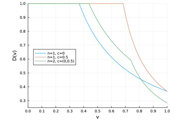
Figure 4: Consumer-optimal demands

We can provide a sharper characterization of the optimal solution when $n=2$. When there are only 2 good for sale, it is without loss to normalize $c_{1}=0$, so the model is parametrized only by $c_{2}$, which we call $c$. It will be useful to consider the limit as the set of values becomes more refined. For this purpose, we define:

$$\Delta\triangleq\min_{k}\{v_{k+1}-v_{k}\}.$$

Proposition 5 (Optimal prices with two goods)

When $n=2$, there exists $\bar{c}$ such that in the consumer-optimal distribution of values, the seller bundles the goods ($p_{1}=p_{2}$) if and only if $c\leq\bar{c}$. Furthermore, as $\Delta\to 0$, we have that $\bar{c}\to\frac{v_{K}}{1+e}$.

This result can be compared with Haghpanah and Hartline (2021), which discusses conditions under which bundling is optimal for the seller. Figure 5 plots the prices the seller charges against the consumer-optimal distribution as a function of $c$, in the limit where $V=[0,1]$. We can see that when the goods have a similar cost, it is optimal to force the seller to bundle the goods together, but as $c$ increases above $\overline{c}=\frac{1}{1+e}$, the price of good 1 falls while the price for good 2 rises.

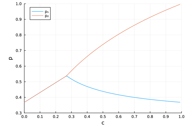
Figure 5: Prices under consumer-optimal demand

5 Effects of Segmentation

With the previous results in hand, we return to the topic of market segmentations. First, we characterize the extreme points of $X_{p}$ in the multigood setting. Then, we discuss how segmentation can improve consumer surplus and lower prices in both interior and extremal markets.

5.1 Extremal Markets

We begin by constructing the class of markets that will be extremal. Consider a subset $S\subseteq V$, and let $D_{r}^{S}$ be the demand defined by (4) but with $S$ taking the place of $V$.

Theorem 2 (Extreme points of $X_{p}$)

Market $x$ is an extreme point of $X_{p}$ if and only if the demand function is given by $D_{r}^{S}$ for some $S\subseteq V$ and $r$ such that $r_{i}\leq p_{i}\leq r_{i+1}$ for all $i$.

That is, the extreme points of $X_{p}$ are all markets of the form $D_{r}^{S}$ where $p$ is an optimal price vector. Intuitively, these markets induce the greatest amount of indifference to the seller.

Proof.

($\Rightarrow$). We first show if $x\in X_{p}$ is an extreme point, then every $v_{k}\in\operatorname{supp}(x)$ is an optimal price for some good $i$. To prove this, suppose there is a $v_{k}$ such that $x(v_{k})>0$, but, for every $i$,

$$v_{k}\notin\operatorname*{arg\,max}_{p_{i}}\Pi_{i}(x,p_{i}).$$

Consider the following market segmentation with uniform distribution and binary support in markets $\{x_{-},x_{+}\}$ defined as follows:

$$D_{x_{-}}(v)=\begin{cases}D(v)&v\neq v_{k}\\ D(v_{k})-\epsilon&v=v_{k}\end{cases};\quad\quad D_{x_{+}}(v)=\begin{cases}D(v)&v\neq v_{k}\\ D(v_{k})+\epsilon&v=v_{k}\end{cases}$$

The segmentations clearly conform to the aggregate market. Furthermore, if $\epsilon$ is small enough, then we continue to have that for all $i$,

$$v_{k}\notin\operatorname*{arg\,max}_{p_{i}}\Pi_{i}(x_{-},p_{i})\text{ and }v_{k}\notin\operatorname*{arg\,max}_{p_{i}}\Pi_{i}(x_{+},p_{i}).$$

Hence, $x_{+},\ x_{-}\in X_{p},$ contradicting that $x$ is an extreme point. Thus, every extreme point satisfies:

$$D_{x}(v_{k})=\frac{\Pi_{i}(x,p_{i})}{v_{k}-c_{i}},$$

for some $i$. To finish the proof, we need to show that the constants $\Pi_{i}(x,p_{i})$ are given by (5). $\Pi_{1}(x,p_{1})=A_{1}$ is immediate, since, by the previous result, $\underline{p}_{1}^{x}=\min\{\operatorname{supp}(x)\}$. Additionally, for any $i$ such that $\overline{p}_{i}^{x}=\underline{p}_{i+1}^{x}$ (or $c_{i}=c_{i+1}$), we have:

$$\frac{\Pi_{i+1}(x,p_{i+1})}{\overline{p}_{i}^{x}-c_{i+1}}=\frac{\Pi_{i}(x,p_{i})}{\overline{p}_{i}^{x}-c_{i}}\implies\Pi_{i+1}(x,p_{i+1})=\Pi_{i}(x,p_{i})\cdot\frac{\overline{p}_{i}^{x}-c_{i}}{\overline{p}_{i}^{x}-c_{i+1}}.$$

Proving $\Pi_{i}(x,p_{i})=A_{i}$ is thus equivalent to showing that $\overline{p}_{i}^{x}=\underline{p}_{i+1}^{x}$ whenever $c_{i}<c_{i+1}$. Suppose otherwise, and let $i$ be the smallest index where this fails. Consider the following segmentation, again with uniform distribution over binary support:

$$D_{x_{-}}(v)=\begin{cases}D_{x}(v)&v<\underline{p}_{i+1}^{x}\\ \kappa D_{x}(v)&v\geq\underline{p}_{i+1}^{x}\end{cases};\quad\quad D_{x_{+}}(v)=\begin{cases}D_{x}(v)&v<\underline{p}_{i+1}^{x}\\ (2-\kappa)D_{x}(v)&v\geq\underline{p}_{i+1}^{x}\end{cases},$$

where $\kappa<1$. We claim that if $\kappa$ is sufficiently close to 1, $x_{-},x_{+}\in X_{p}$.

Take $x_{-}$ (a similar argument works for $x_{+}$). If any prices changed, it is of some good in $\{i+1,\dots,n\}$. But, for any good $j\geq i+1$ and $v_{k}<\underline{p}_{i+1}^{x}$,

$$\Pi_{j}(x,p_{j})\geq\Pi_{j}(x,\underline{p}_{i+1}^{x})>\Pi_{j}(x,\overline{p}_{i}^{x})\geq\Pi_{j}(x,v_{k}),$$

where the first inequality comes from optimality of price $p_{j}$, and the next two follow from Lemma 2 of Appendix B. Thus, for $\kappa$ sufficiently close to 1, we have $x_{-},x_{+}\in X_{p}$, a contradiction.

($\Leftarrow$). By Theorem 1, $D_{p}$ first-order stochastic dominates every element of $X_{p}$. Hence, it cannot be written as the convex combination of two elements in $X_{p}$. Similarly, $D_{p}^{S}$ first-order stochastic dominates every element of $X_{p}$ with support contained in $S$.    

Example.

Let $x^{\ast}$ be the uniform distribution over $V=\{1,2,3,4,5\}$ and $c=(0,2)$. The unique aggregate monopoly prices are $p^{\ast}=(3,4)$. Then $X_{p^{\ast}}$ is non-empty, and its extreme points are the distributions $D_{r}^{S}$ where $r_{2}\in\{3,4\}$, $r_{1}\in\{1,2,\dots,r_{2}\}$, and $\{r_{1},r_{2}\}\subseteq S\subseteq V$.

Theorem 2 characterizes the extremal markets. We now show that the welfare implication of segmenting markets is different when considering extremal and interior markets.

5.2 Market Segmentation and Price Changes: Interior Markets

With the previous results in hand, we can now ask when it is possible to find segmentations that decrease the price of every good relative to the prices that would prevail in the aggregate market. In this section, we assume that in every market, the lowest possible prices will prevail.

We begin by showing that, if a segmentation does not provide strict incentives for the seller to change its prices, then this segmentation is weakly beneficial for consumers.

Proposition 6 (Weakly beneficial segmentations)

Every market segmentation $\sigma$ with support in $X_{p^{\ast}}$ generates the same profits and weakly lower prices relative to the aggregate market in every segment.

Proof.

The proof of this proposition is straightforward. For any market $x\in X_{p^{\ast}}$ we have that (by definition) $p^{\ast}$ is an optimal price in market $x$, so:

$$\underline{p}^{x}_{i}\leq p_{i}^{\ast}\text{ for every }i\in\{1,...,n\}.$$

Since, by assumption, the lowest possible prices prevail, all prices are weakly lower.    

We thus have that segmenting a market $x^{*}$ using the extreme points of $X_{p^{*}}$ can only increase consumer surplus. In fact, we can provide conditions such that this improvement is strict. Denote by $p^{FB}$ the efficient price vector:

$$p^{FB}_{i}=\min\{v\in V\mid v>c_{i}\}.$$

A price $p$ is inefficient if, for some $i$, $p_{i}>p_{i}^{FB}$. If the aggregate market $x^{\ast}$ is in the interior of $X_{p^{\ast}}$, and $p^{\ast}$ is inefficient, then there is a binary segmentation which strictly lowers prices.

Proposition 7 (Strictly beneficial segmentations)

Suppose that $x^{\ast}\in\operatorname{int}(X_{p^{\ast}})$ and $p^{\ast}$ is inefficient. Then there exists a binary segmentation which weakly decreases the price of every good, and strictly decreases the price of some good.

Proof.

Denote by $i_{0}$ the index of the cheapest good that is inefficiently supplied:

$$i_{0}\triangleq\min\{i\mid p_{i}>p_{i}^{FB}\}.$$

Let $r$ be the price vector identical to $p^{\ast}$ except at $i_{0}$, where $r_{i_{0}}=p_{i_{0}}^{FB}$.

We begin by showing that $D_{r}$ is an extreme point of $X_{p^{\ast}}$. We know $r_{i_{0}}<p^{\ast}_{i_{0}}\leq p^{\ast}_{i_{0}+1}=r_{i_{0}+1}$, so $p^{\ast}_{i_{0}}$ is still an optimal price for good $i_{0}$. Additionally, by construction, good $i_{0}-1$ is efficiently supplied, meaning that:

$$r_{i_{0}-1}=p^{*}_{i_{0}-1}=p_{i_{0}-1}^{FB}\leq p_{i_{0}}^{FB}=r_{i_{0}}$$

Thus, $p^{\ast}_{i_{0}-1}$ is still an optimal price for good $i_{0}-1$, and $D_{r}$ is an extreme point of $X_{p^{*}}$.

Consider now a market segmentation with binary support. The first market is $D_{r}$ with $\sigma(D_{r})=\epsilon$, and the second market $x$ satisfies:

$$D_{x}=\frac{D^{*}-\epsilon D_{r}}{1-\epsilon}.$$

If $x^{\ast}\in\text{int}(X_{p^{*}})$, then for a small enough $\epsilon$ we have that $x\in\text{int}(X_{p^{*}})$. It follows from Proposition 6 that in this segmentation, all prices are weakly lower. Additionally, in market $D_{r}$, the price of good $i_{0}$ is strictly lower. Hence, there is a segmentation which strictly lowers prices.    

The proposition tells us that, generically, it is possible to achieve Pareto improvements with binary segmentations, a result also shown in a more general setting by Haghpanah and Siegel (2023). Importantly, not only does this segmentation strictly increase aggregate consumer surplus, it weakly increases every individual consumer’s surplus.

5.3 Market Segmentation and Price Changes: Extremal Markets

In the previous section we showed that segmenting an interior can be done without harming any consumers and without increasing profits. The proof, however, relies on the ability to segment the market into extremal markets. This approach does not work for extremal markets. We can first verify that, for any extremal market, any non-trivial segmentation necessarily increases profits.

Proposition 8 (Prices and Profits in Segmentations of Extremal Markets)

If $x$ is an extremal market, then there is no (non-trivial) market segmentation that induces weakly lower prices in every segment. Furthermore, any segmentation increases profits.

Proof.

Consider an extremal market $D_{r}$, and any market segmentation $\sigma$. Following Theorem 1, if $\underline{p}^{x}\leq r$ for every $x\in\operatorname{supp}(\sigma)$, then $D_{r}$ first-order stochastically dominates each such $x$. We thus have that it is not possible to write $D_{r}$ as a linear combination of markets in $\operatorname{supp}(\sigma)$.    

This proposition shows that the logic behind interior markets stated in Proposition 6 does not go through. In fact, the effects of segmenting go almost in the opposite direction. It is not exactly the opposite direction because segmenting an extremal market might still lead to lower prices in some segments. We next show that, despite prices increasing for some markets and profits increasing, sometimes it is possible to find segmentations of extremal markets that are beneficial for aggregate consumer surplus.

Proposition 9 (Surplus in extremal market segmentations)

There are segmentations of extremal markets that lead to higher aggregate consumer surplus. Furthermore, there may be extremal markets for which no binary segmentation, but at least one non-binary segmentation, increases aggregate consumer surplus.

To prove the proposition it suffices to illustrate with an example. Return to the example of Figure 1, where $V=\{1,2,3\}$, $c=(0,\varepsilon)$, and the aggregate market is given by

$$D_{x^{*}}=\left(1,\frac{1}{2},\frac{1}{3}\right)$$ (7)

(marked with a white circle in the figure). Consider the segmentation of the aggregate market into the following three extremal markets:

$$D_{1}=\left(1,\frac{1}{2-\varepsilon},\frac{1}{3-\varepsilon}\right);\quad D_{2}=\left(1,1,(2-\varepsilon)\frac{1}{3-\varepsilon}\right);\quad D_{3}=(1,1,1).$$

The three markets consist of the blue and two gray circles in Figure 1. It is then straightforward to verify that the aggregate consumer surplus has increased relative to the no segmentation case when $\varepsilon$ is small enough. For this simply note that as $\varepsilon\to 0$, we have that $\sigma(x_{1})\to 1$, but the price in market $D_{1}$ are strictly smaller, so the consumer surplus generated is strictly larger. Notice that, although aggregate consumer surplus is higher, in some markets prices have increased relative to $x^{\ast}$, meaning some individual consumers are worse off.

The intuition is as follows: low value buyers tend to decrease the price of all goods. But, relatively more low value buyers are needed to decrease the price of expensive items, since the function $D(v)=\frac{A}{v-c}$ has more mass at the left for higher $c$. This holds even if the difference in cost is only $\varepsilon$ small. Hence, we inevitably “run out” of low value buyers, and some segments must see the price of the cheap good increase.

Proposition 8 shows that it is impossible to segment an extremal market in a way that every price decreases. However, it is possible to keep the price of the most costly good weakly lower.

Proposition 10 (Lower Price of the Good with the Highest Cost)

Take any $x^{\ast}$ and segmentation $\sigma$. There exists a segmentation $\hat{\sigma}$ such that: (a) $\hat{\sigma}$ delivers weakly higher total surplus and consumer surplus, and (b) in every segment $\hat{x}\in\operatorname{supp}(\hat{\sigma})$, $\hat{p}_{n}\leq p_{n}^{\ast}$.

The proof constructs $\hat{\sigma}$ explicitly. This result shows that for segmentations of extremal markets, while increasing some prices in certain segments may be necessary to raise consumer surplus, we can always lower price of at least one good: specifically, the most expensive one.

6 Welfare Analysis

6.1 The Surplus Polytope

We now introduce the surplus polytope, a useful tool for visualizing the space of achievable divisions of surplus. In any segmentation, the monopolist must be receiving at least their aggregate monopoly profit, $\Pi^{\ast}$, the sum of the consumer surplus and profit $U+\Pi$ is bounded above by the maximum social surplus, and consumer surplus is nonnegative. Bergemann et al. (2015) prove that when $n=1$, these are in fact the only restrictions on surplus division, and the entire “surplus triangle” is achievable. When $n>1$, however, this does not generally hold, a fact first shown by Haghpanah and Siegel (2022).

For finite $n$, the space of achievable surplus divisions is a convex polytope. Figure 6 gives an example of a surplus polytope selected to demonstrate the potential complexity of the frontier. A number of points of interest are labeled, which we explain next.

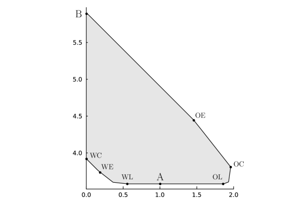
Figure 6: Fully featured surplus polytope. The parameters generating this polytope are: $V=\{1,\dots,5\}$, $x^{\ast}=(0.1,0.3,0.2,0.2,0.2)$, and $c=(0,1.65,1.9)$.

Point A is the aggregate market outcome, and B is the outcome of perfect price discrimination. OC is the outcome which is optimal for the consumer. Point OL represents the maximum consumer surplus that can be attained while keeping the profits at $\Pi^{\ast}$. We know profits remain constant if and only if the support of the segmentation is in $X_{p^{*}}$, so it is the “optimal local” outcome. OE is the “optimal efficient” outcome, achieving the highest consumer surplus along the efficient frontier. Similarly, WL represents the worst local segmentation, WE is the point with the worst (lowest) efficiency, and WC achieves the lowest profit along the 0 consumer surplus line.

For a particular aggregate market, the surplus polytope may not contain all the features seen in Figure 6. For example, Figure 7 plots the exact surplus polytope when $V=\{1,2,3\}$ and $c=(0,\frac{1}{3})$ for two aggregate markets. We now describe and provide an intuition for these examples. In particular, we explain why the complete triangle of feasible surplus pairs is not attainable.

In 7(a) we show the surplus pairs that are attainable when the aggregate market is (7) (we recall that this is the white dot in Figure 1). We previously explained why in this market it is possible to increase aggregate consumer surplus, although this necessarily also increases profits: this was the argument provided for the proof of Proposition 8. On the lower frontier, WL, WE, and WC all coincide. The reason is that the for the aggregate market there are multiple optimal prices. By choosing different optimal prices the seller can change consumer surplus without changing profits. In fact, $p=(3,3)$ is an optimal price in the optimal market and this leaves the seller with zero consumer surplus. Hence, the multiple levels of consumer surplus consistent with the profits generated by the aggregate market are not a consequence of market segmentation changing consumer surplus but an effect of the multiplicity of optimal prices in the aggregate market.

Figure 7(b) shows the polytope when

$$D_{x^{\ast}}=\left(1,\frac{1}{2},\frac{2-c_{2}}{2}\frac{1}{3-c_{2}}\right).$$ (8)

This corresponds to the red dot in Figure 1. As before, OL differs from OC, which means that market segmentation can increase consumer surplus despite this being an extremal market. In contrast to the previous example, here WE and WC coincide but differ from WL. The intuition is simple. In the aggregate market the consumer is guaranteed to have some consumer surplus despite the choice seller’s price (as long as it is an optimal price). Hence, reducing some the consumer surplus to zero (as it is always possible) requires some market segmentation and market segmentation always increases profits (Proposition 8). Hence, the lower-left corner of the feasible surplus pairs is not attainable by market segmentation.

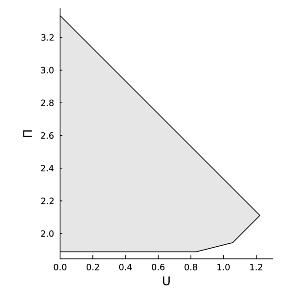
(a) Polytope when the aggregate market is (7) (this corresponds to the white dot in Figure 1).

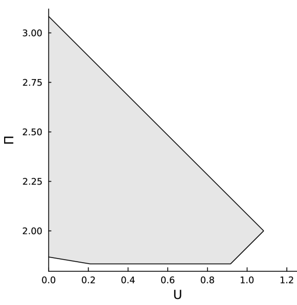
(b) Polytope when the aggregate market is (8) (this corresponds to the red dot in Figure 1).

Figure 7: Surplus polytope with $V=\{1,2,3\}$ and $c=(0,\frac{1}{3})$

The surplus polytope also allows us to restate two results from the previous section in a visual manner. Proposition 7 is the statement that, for any $x^{\ast}$ strictly in the interior of $X_{p^{\ast}}$, either A is the bottom right corner of the triangle, or OL (and hence OC) lie to the right of A. Proposition 8 tells us that, if $x^{\ast}$ is an extremal market, then $\text{WL}=\big{(}U(x^{\ast},\overline{p}^{\ast}),\Pi^{\ast}\big{)}$ and $\text{OL}=\big{(}U(x^{\ast},\underline{p}^{\ast}),\Pi^{\ast}\big{)}$ are achieved without segmentation.

6.2 Numerical Calculation of the Boundary

In principle, we can draw the boundaries of the surplus polytope by solving, via an LP, the consumer surplus maximizing (or minimizing) segmentation subject to receiving a particular profit level. However, this is computationally expensive, as it requires tracing over all profit levels from $\Pi^{\ast}$ to $\operatorname{E}_{v\sim x^{\ast}}[v]$. Alternatively, the theory of LP projection, as in Haeusle and Vohra (2023), can be used to derive the shape of the frontier analytically, but this is an algebraically intensive process. Instead, for the labeled points of interest, a slightly more direct computational method can be used to find the labeled points along the frontier.

Consider the following problem. Given a collection $\{x_{j}\}$ of $K$-dimensional vectors, each with value $w_{j}$, along with a $K$-dimensional constraint $x^{\ast}$, we wish to find $\sigma_{j}\geq 0$ to solve:

$$\max_{\sigma}\left[\sum_{j}\sigma_{j}\cdot w_{j}\right]\text{ s.t. }\forall k,\ \sum_{j}\sigma_{j}\cdot x_{j}(k)=x^{\ast}(k),$$ (9)

where $x_{j}(k)$ denotes the $k$-th element of $x_{j}$.

It turns out that we can choose $\{x_{j}\}$ and $\{w_{j}\}$ appropriately to make the solution to this convex optimization the points of interest along the surplus polytope’s frontier.

Proposition 11 (Computable points)

For each of labeled points in Figure 6, there exists a subset of extremal markets $\{x_{j}\}$ and values $\{w_{j}\}$ such that the solution to (9) is a segmentation achieving that point.

Example.

Let $x^{\ast}$ be the uniform distribution over $V=\{1,\dots,5\}$, and $c=(0,2)$. Aggregate monopoly prices are $p^{\ast}=(3,4)$. In the aggregate monopoly market, consumer surplus is 0.8 and profit is 2.6, while the efficient frontier is at 4.2. A consumer surplus maximizing extremal segmentation is given in Table 1.

$\sigma(x)$	$S$	$r$	$x(1)$	$x(2)$	$x(3)$	$x(4)$	$x(5)$
$\frac{2}{5}$	$\{1,2,3,4,5\}$	$(1,4)$	$\frac{1}{2}$	$\frac{1}{6}$	$\frac{1}{12}$	$\frac{1}{12}$	$\frac{1}{6}$
$\frac{2}{5}$	$\{2,3,4,5\}$	$(2,4)$	0	$\frac{1}{3}$	$\frac{1}{6}$	$\frac{1}{6}$	$\frac{1}{3}$
$\frac{1}{5}$	$\{3,4\}$	$(3,4)$	0	0	$\frac{1}{2}$	$\frac{1}{2}$	0
1	$\{1,2,3,4,5\}$	$(3,4)$	$\frac{1}{5}$	$\frac{1}{5}$	$\frac{1}{5}$	$\frac{1}{5}$	$\frac{1}{5}$

Table 1: Consumer-optimal Segmentation of $x^{\ast}$

This segmentation delivers a consumer surplus of 1.5 and profit of 2.6, for a total surplus of 4.1. Note that the consumer-optimal segmentation is not unique.

Proposition 11 demonstrates how Theorem 2 enables not only theoretical analysis of the segmentation problem, but also computational results. Without it, we would potentially have to search over the entire space of markets $\Delta V$, or face the possibility that the segmentation we seek contains an infinite number of segments.

6.3 Achievability of Surplus Triangle

Finally, we can ask ourselves when the corners of the surplus polytope coincide with the corners of the surplus triangle à la Bergemann et al. (2015).

Proposition 12 (Efficient consumer maximization)

If there is a segmentation such that the consumer surplus maximizing segmentation is efficient, then $p_{i}^{\ast}\leq p_{i+1}^{FB}$ whenever $c_{i}<c_{i+1}$.

This proposition tells us that a necessary condition for the lower right corner to be achievable is that the optimal aggregate monopoly prices are not too high relative to costs. Note that, as a necessary condition, the converse is not true; an aggregate market can satisfy this condition but still be unable to achieve the lower right corner.

We can write an analogous necessary condition for the opposite corner $(U,\Pi)=(0,\Pi^{\ast})$ to be achievable. This condition turns out to be more restrictive: it requires that the seller price all goods as high as possible in the aggregate market, except those with the smallest cost.

Proposition 13 (Profit and surplus minimization)

If there is a segmentation such that $(U,\Pi)=(0,\Pi^{\ast})$, then for all $i$ such that $c_{i}>c_{1}$, $p_{i}^{\ast}=v_{K}$.

Combining these two proposition generates a necessary condition for the entire surplus triangle to be achievable. An interesting implication is that if there are 3 goods with distinct costs and non-trivial pricing decisions, no aggregate markets can achieve the entire surplus triangle.

Corollary 3 (Unachievability of surplus triangle)

If there is a good $i$ such that $c_{1}<c_{i}<c_{i+1}<v_{K-1}$, there exists no $x^{\ast}\in\Delta V$ such that the entire surplus triangle is achievable by segmentation.

In other words, in order for the entire surplus triangle to be achievable, there are effectively at most two goods. Thus, the result of Bergemann et al. (2015) that the entire surplus triangle is always achievable is a special feature of the single good case.

7 Conclusion

This paper extends the results of Bergemann et al. (2015) to the general finite good case by characterizing the extreme points of nonlinear pricing markets. In doing so, we are able to analyze how third degree price discrimination, when used in conjunction with second degree price discrimination, affects consumer surplus, profits, and prices. We hope that further work will yield a similar result for the case of continuous quality production, although a new approach will be required.

In an age where sellers have access to an increasing amount of information about potential consumers, it is natural to worry about the welfare impacts of allowing sellers to segment consumers into precisely drawn markets. Our findings show that when investigating the potential welfare impact of segmentation, it is sufficient to limit attention to a few very special distributions, even when producers combine second and third degree price discrimination. The exact outcome of segmentation, however, naturally depends on how the segments are drawn. More work is required to understand the welfare implications of segmentation as it arises endogenously and in practice.

Appendix A Continuous Type and Quality

Extending our main results to a continuous type set is relatively straightforward, as the demand function given by (4) is well-defined for both continuous and discrete $V$. Hence, Theorem 2 applies exactly as stated, with the distributions $D_{r}^{S}$ now being continuous. These distributions are still piecewise generalized Pareto, with up to $n$ pieces, and the start and end points of each piece determine the possible prices. However, it is no longer generally possible to explicitly write out the extremal segmentations which achieve particular surplus divisions, as they may have infinitely many segments.

Generalizing to continuous $q$ is more difficult. Suppose that, instead of having $n$ goods, the producer is able to select any quality level $q\in\mathbb{R}_{+}$, with the cost of producing a good of quality $q$ given by the convex function $c(q)$. This is equivalent to taking the limit as $n\rightarrow\infty$ and renormalizing the utilities. Theorem 2 is now vacuous, as generically, $X_{p}$ consists of a single point.

For simplicity, let us assume an isoelastic cost function, $c(q)=\frac{q^{\eta}}{\eta}$ for some $\eta>0$, and normalize $V=[0,1]$. As before, our approach is to find the consumer-optimal distribution of values, then conjecture that the family of distributions arising from solving this problem, varying the support, are sufficient to achieve all feasible surplus divisions. Unlike (4), where the distributions vary in both support and shape, since we have fixed the elasticity of the cost function, the resulting distributions are defined fully by their support.

Unfortunately, we are only able to characterize the relevant distributions as the solution to an optimal control problem. When $\eta=2$, we can simplify the problem further, but the solution is still a non-elementary function. As a result, it is difficult to prove that segmentations consisting of only these distributions are sufficient to recover the entire space of feasible surplus divisions. For now, it remains a conjecture.

A.1 Continuous Quality via Optimal Control

Consider a single consumer who chooses a Myerson-regular distribution $F(v)$ over $[0,1]$. After observing $F$, the producer selects a mechanism $\mathcal{M}:v\rightarrow(q,p)$ giving, for every value $v$, the quality produced and the price charged to the consumer. The payoff to the consumer is $vq-p$, and to the producer is $p-c(q)=p-\frac{q^{\eta}}{\eta}$. By standard results, the revenue-maximizing truthful mechanism solves point-wise

$$\phi(v)=c^{\prime}(q(v))\implies q(v)=\phi(v)^{\frac{1}{\eta-1}},$$

where $\phi(v)=v-\frac{1-F(v)}{f(v)}$ is the virtual value. Incentive-compatibility then pins down the consumer surplus at each point of $\operatorname{supp}(F)=[\underline{v},\overline{v}]$:

$$U(v)=\int_{\underline{v}}^{\overline{v}}q(x)\ dx=\int_{\underline{v}}^{\overline{v}}\left(x-\frac{1-F(x)}{f(x)}\right)^{\frac{1}{\eta-1}}\ dx.$$

The total consumer surplus is

$$\operatorname{E}_{v\sim F}\Big{[}U(v)\Big{]}=\int_{\underline{v}}^{\overline{v}}U(v)f(v)\ dv+\operatorname{P}(v=\overline{v})U(\overline{v}).$$ (10)

The consumer maximizes the above expression over $F$. Using Pontryagin’s Maximum Principle (PMP), we can characterize the optimal $F$ as the solution to an optimal control problem.

Proposition 14 (Consumer-optimal distribution with continuous quality)

Let $F$ be the solution to the consumer maximization problem with continuous $q$. Then for some costate function $\mu(v)$ and lower bound $\underline{v}=\inf\{\operatorname{supp}(F)\}$,

$$\frac{dF}{dv}=f(v),\ \frac{dU}{dv}=\left(v-\frac{1-F(v)}{f(v)}\right)^{\frac{1}{\eta-1}}$$ (11)

$$\frac{d\mu}{dv}=-\frac{1-F(v)}{f(v)(\eta-1)}\left(v-\frac{1-F(v)}{f(v)}\right)^{\frac{1}{\eta-1}-1}$$ (12)

$$\mu(v)+\frac{(1-F(v))^{2}}{f(v)^{2}(\eta-1)}\left(v-\frac{1-F(v)}{f(v)}\right)^{\frac{1}{\eta-1}-1}+U(v)=0$$ (13)

$$F(\underline{v})=U(\underline{v})=0,\ \mu(1)=-U(1)$$ (14)

Line 11 is state evolution, 12 is costate evolution, 13 is PMP, and 14 are terminal conditions.

As in the finite good case, these equations define a family of distributions with varying support sets, and the consumer-optimal distribution will be a member of this family. This result can be contrasted with Bergemann et al. (2023), where the authors find that the distribution which maximizes the ratio of consumer surplus to total surplus is a Pareto distribution with shape $\frac{\eta}{\eta-1}$.

Observe that $\mu$ and $U$ can be combined into a single variable $\hat{\mu}:=\mu+U$, and thereby reduce the number of variables and equations. This simplifies the problem both computationally and theoretically, as we will see below, although $\hat{\mu}$ is somewhat harder to interpret.

Example.

Take $\eta=2$. Rewrite the system using the augmented costate $\hat{\mu}$. The evolution equation for this variable is

$$\frac{d\hat{\mu}}{dv}=\phi(v)-\frac{1-F(v)}{f(v)}=2\phi(v)-v,$$

where $\phi(v)$ is the virtual value. Similarly, PMP becomes

$$\hat{\mu}=-(v-\phi(v))^{2}\implies\frac{d\hat{\mu}}{dv}=2(\phi(v)-v)\left(1-\frac{d\phi}{dv}\right).$$

Setting these two expressions equal to each other yields

$$\frac{d\phi}{dv}=\frac{1}{2}\cdot\frac{v}{v-\phi(v)}.$$

This is a homogeneous first order ODE, and thus admits an implicit solution:

$$\log\Big{(}v^{2}+2\phi(v)^{2}-2v\phi(v)\Big{)}-2\tan^{-1}\left(\frac{2\phi(v)}{v}-1\right)+\frac{\pi}{2}=0.$$ (15)

The solution to this equation over $[0,1]$ is plotted in Figure 8.

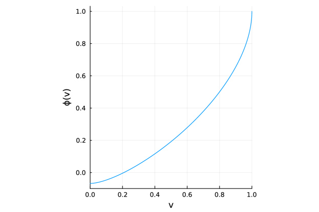
Figure 8: Solution to (15) over $[0,1]$

Given a choice of support, we can recover the corresponding distribution by converting $\phi(v)$ to the hazard rate and applying the hazard rate transformation.

A natural conjecture, to mirror the main text, is that segmentations consisting of the distributions defined by Proposition 14, with varying support, achieve every feasible surplus division. However, since these distributions are defined only indirectly, as the solution to an optimal control problem (and, as the example demonstrates, are non-elementary functions), it is difficult to directly prove anything about them. We leave this as a direction for possible future research.

Appendix B Proofs

We begin by presenting a few useful lemmas.

Lemma 1 (Profit-preserving segmentations)

A segmentation $\sigma$ delivers profit $\Pi^{\ast}$ to the seller if and only if the support of $\sigma$ is contained in $X_{p^{\ast}}$.

Proof.

($\Rightarrow$). Suppose that for some $\hat{x}\in\operatorname{supp}(\sigma)$, $\hat{x}\notin X_{p^{\ast}}$, meaning $\Pi(\hat{x},\hat{p})>\Pi(\hat{x},p^{\ast})$. Then:

$$\sum_{x\in\operatorname{supp}(\sigma)}\sigma(x)\Pi(x,p^{x})>\sum_{x\in\operatorname{supp}(\sigma)}\sigma(x)\Pi(x,p^{\ast})=\Pi^{\ast},$$

which is a contradiction.

($\Leftarrow$). If $\operatorname{supp}(\sigma)\subset X_{p^{\ast}}$, then $p^{\ast}$ is a profit-maximizing price for every segment, and aggregate profits are equivalent to charging $p^{\ast}$ in the aggregate market.    

Lemma 2 (Co-monotonicity of prices and costs)

For any $i,j$ such that $c_{i}>c_{j}$ and $v,\hat{v}$ such that $v>\hat{v}$ (or $c_{i}<c_{j}$ and $v<\hat{v}$):

$$\Pi_{i}(x,v)\leq\Pi_{i}(x,\hat{v})\implies\Pi_{j}(x,v)<\Pi_{j}(x,\hat{v}).$$

Proof.

We have:

$$\Pi_{i}(x,v)\leq\Pi_{i}(x,\hat{v})\implies\frac{D_{x}(v)}{D_{x}(\hat{v})}\leq\frac{\hat{v}-c_{i}}{v-c_{i}}<\frac{\hat{v}-c_{j}}{v-c_{j}}\implies\Pi_{j}(x,v)<\Pi_{j}(x,\hat{v}),$$

as desired. The case of $c_{i}<c_{j}$ can be proven with a similar argument by inverting the ratios.    

Lemma 3 (Consumer surplus in continuous extremal markets)

Suppose $V=[0,1]$. For any $x=D_{p}$:

$$U(x,p)=\sum_{i=1}^{n}\left[iA_{i}\log\frac{p_{i+1}-c_{i}}{p_{i}-c_{i}}\right]$$

Proof.

The consumer surplus from selling good $i$ to consumers with valuations $v\in[p_{j},p_{j+1})$ is:

$$A_{j}\int_{p_{j}}^{p_{j+1}}\frac{v-p_{i}}{(v-c_{j})^{2}}\ dv=A_{j}\left(\log\frac{p_{j+1}-c_{j}}{p_{j}-c_{j}}-\frac{(p_{i}-c_{j})(p_{j+1}-p_{j})}{(p_{j+1}-c_{j})(p_{j}-c_{j})}\right).$$

The total consumer surplus is the above expression summed over all $i$ and $j\geq i$, plus the consumer surplus of the mass point at the end, $\frac{A_{n}}{1-c_{n}}\sum_{i}(1-p_{i})$. Summing everything together, we get:

$$U(x,p)=\sum_{i=1}^{n}\left[iA_{i}\log\frac{p_{i+1}-c_{i}}{p_{i}-c_{i}}+\frac{A_{n}}{1-c_{n}}(1-p_{i})-\sum_{j\geq i}A_{j}\frac{(p_{i}-c_{j})(p_{j+1}-p_{j})}{(p_{j+1}-c_{j})(p_{j}-c_{j})}\right].$$

We claim that the non-logarithmic terms cancel out. To see this, fix an $i$, then take the difference between the middle term and the $j=n$ summand of the last term:

$$\frac{A_{n}}{1-c_{n}}\left[1-p_{i}-\frac{(p_{i}-c_{n})(1-p_{n})}{p_{n}-c_{n}}\right]=\frac{A_{n}}{p_{n}-c_{n}}(p_{n}-p_{i})=\frac{A_{n-1}}{p_{n}-c_{n-1}}(p_{n}-p_{i}).$$

Repeat this recursively for $j=n-1,\dots,i$, and at the last step the sum becomes 0.    

Proof of Proposition 5.

Consider the limit where $V=[0,1]$. Lemma 3 reduces finding the optimal $p$ to a constrained optimization problem, subject to $p_{1}\leq p_{2}$. The KKT conditions are:

$$\mu=\log\frac{p_{2}}{p_{1}}+2\left(1-\frac{c}{p_{2}}\right)\log\frac{1-c}{p_{2}-c}-1=\frac{p_{1}}{p_{2}}-2\left(\frac{p_{1}c}{p_{2}^{2}}\right)\log\frac{1-c}{p_{2}-c}$$ (FOC)

$$\mu(p_{2}-p_{1})=0.$$ (CS)

We can check when $p_{1}=p_{2}$ is a solution. Plugging in $p_{1}=p_{2}=p$ yields $p=\frac{1}{e}(1-c)+c$. Dual feasibility then requires that:

$$\mu=\frac{2(1-c)}{1+(e-1)c}-1\geq 0\iff c\leq\frac{1}{1+e}.$$

This completes the proof for the limit case. When $V$ is discrete, the logarithm in Lemma 3 is replaced by a discrete approximation function; however, one can verify that a similar argument holds, although the bundling breakpoint $\overline{c}$ will be different.    

Proof of Proposition 10.

Let $\{x_{1},\dots,x_{J}\}$ be the support of $\sigma$. We construct $\hat{\sigma}$ to have support $\{\hat{x}_{1},...,\hat{x}_{J}\}$, with $\sigma(x_{j})=\hat{\sigma}(\hat{x}_{j})$. Each $\hat{x}_{j}$ is defined as follows:

$$D_{\hat{x}_{j}}(v_{k})=\begin{cases}D_{x_{j}}(v_{k})&v_{k}<p^{*}_{n}\\ D_{x^{*}}(v_{k})\frac{D_{x_{j}}(p_{n}^{\ast})}{D_{x^{*}}(p_{n}^{*})}&v_{k}\geq p^{*}_{n}\end{cases}$$

We first verify that segmentation $\hat{\sigma}$ is feasible. For every $v_{k}\geq p^{*}_{n}$ we have that:

$$\sum_{j=1}^{J}\hat{\sigma}(\hat{x}_{j})D_{\hat{x}_{j}}(v_{k})=D_{x^{*}}(v_{k})\sum_{j=1}^{J}\sigma(\hat{x}_{j})\frac{D_{x_{j}}(p_{n}^{*})}{D_{x^{*}}(p_{n}^{*})}=D_{x^{*}}(v_{k}),$$

where the first equality is the definition of $D_{\hat{x}_{j}}$ and the second comes from the fact that $\sigma$ is a valid segmentation. For $v_{k}<p_{n}^{\ast}$, $\hat{x}_{j}$ and $x_{j}$ coincide. Thus, $\hat{\sigma}$ aggregates to $x^{\ast}$.

Next, we claim that if $p$ and $\hat{p}$ are optimal prices in markets $x_{j}$ and $\hat{x}_{j}$, respectively, then:

$$\hat{p}_{i}\leq\min\{p_{i},p_{n}^{*}\}\text{ for every }i\in\{1,...,n\}.$$ (16)

To see this, note that for all $v_{k}\geq p_{n}^{\ast}$:

$$\Pi_{i}(\hat{x}_{j},v_{k})-\Pi_{i}(\hat{x}_{j},p_{n}^{\ast})=\frac{D_{x_{j}}(p_{n}^{\ast})}{D_{x^{\ast}}(p_{n}^{\ast})}\Big{(}\Pi_{i}(x^{\ast},v_{k})-\Pi_{i}(x^{\ast},p_{n}^{\ast})\Big{)}\leq 0.$$

The equality follows from the construction of $\hat{x}_{j}$ and the inequality from Lemma 2.

Thus, the optimal price of every good in market $\hat{x}_{j}$ is at most $p_{n}^{\ast}$. But, for any $v_{k}<p_{n}^{\ast}$, $\hat{x}_{j}$ and $x_{j}$ coincide. So, if $p_{i}<p_{n}^{\ast}$, then $\hat{p}_{i}=p_{i}$. This proves (16). Since all prices in $\hat{x}_{j}$ are lower than in $x_{j}$, total surplus and consumer surplus must also be weakly higher.    

Proof of Proposition 11.

By making $\{x_{j}\}$ a subset of the extremal markets $D_{p}^{S}$ and $x^{\ast}$ the aggregate market, the constraint in (9) reduces to the majorization constraint. The problem, then, is choosing the relevant subset of extremal markets $D_{p}^{S}$, and picking $w_{j}$ so that the solution is the desired point.

For WE and OC, we can take $\{x_{j}\}$ to be the full set of extremal markets. By Lemma 1, for WL and OL, the appropriate restriction is to the extreme points of $X_{p^{\ast}}$. For OE, we take the set of extremal markets $x$ such that $\underline{p}_{x}$ is efficient. Finally, for WC, we restrict to those extremal markets $x=D_{r}^{S}$ such that $\overline{p}^{x}=(\max\{S\},\dots,\max\{S\})$.

Next, we can identify the prices that will prevail in each market. For OL, OC, and OE, since we are maximizing consumer surplus or efficiency, that will be $\underline{p}^{x}$. For WL, WE, and WC, where the opposite is true, it will be $\overline{p}^{x}$.

Finally, since we have identified the prices $p_{j}$ which prevail in each market $x_{j}$, $w_{j}$ can be directly assigned as the objective, which will be $U(x_{j},p_{j})$ (or $-U(x_{j},p_{j})$) for all points except WE, where it will be $U(x_{j},p_{j})+\Pi(x_{j},p_{j})$.    

Proof of Proposition 12.

We prove by contradiction. Suppose the consumer-optimal extremal segmentation $\sigma$ is efficient, but $p_{i}^{\ast}>p_{i+1}^{FB}$ for some $i$ such that $c_{i}<c_{i+1}$. By Lemma 1, for all segments $x=D_{r}^{S}$, $x\in X_{p^{\ast}}\implies p_{i}^{\ast}\leq r_{i+1}$. Since the segmentation maximizes consumer surplus, $p_{i+1}^{x}=\underline{p}_{i+1}^{x}=r_{i+1}$. Thus, $p_{i+1}^{x}>p_{i+1}^{FB}$ for all segments $x$. However, there must be some segment $\hat{x}$ such that $p_{i+1}^{FB}\in\operatorname{supp}(\hat{x})$. By efficiency, in this segment, $p_{i+1}^{\hat{x}}=p_{i+1}^{FB}$, a contradiction.    

Proof of Proposition 13.

Consider an extremal segmentation $\sigma$ achieving $(0,\Pi^{\ast})$. Zero consumer surplus means that in every segment, the price of every good is $\max\{S\}$. Take any segment $x=D_{r}^{S}$ such that $v_{K}\in S$. For all $i$ such that $c_{i}>c_{1}$, $\overline{p}_{1}^{x}\leq r_{i}\implies r_{i}=v_{K}$. By Lemma 1, since $\sigma$ delivers profit $\Pi^{\ast}$, $x\in X_{p^{\ast}}\implies p_{i}^{\ast}\in[r_{i},r_{i+1}]\implies p_{i}^{\ast}=v_{K}$.    

Proof of Proposition 14.

Maximizing equation 10 over $F$ is an optimal control problem, where $f$ is the control variable and $F,U$ are the state variables. The instantaneous reward is $U(v)f(v)$ and the terminal reward is $(1-F(\overline{v}))U(\overline{v})$. The state variables evolve according to

$$\frac{dF}{dv}=f(v),\ \frac{dU}{dv}=\left(v-\frac{1-F(v)}{f(v)}\right)^{\frac{1}{\eta-1}}.$$

Let $\mu_{1},\mu_{2}$ be the costates associated with $F,U$ respectively. The Hamiltonian is

$$H(\mu_{1},\mu_{2},F,U,f,v)=\mu_{1}(v)f(v)+\mu_{2}(v)\left(v-\frac{1-F(v)}{f(v)}\right)^{\frac{1}{\eta-1}}+U(v)f(v).$$

The adjoint terminal conditions are $\mu_{1}(\overline{v})=-U(\overline{v})$ and $\mu_{2}(\overline{v})=1-F(\overline{v})$, and the costate evolution equations are

$$\frac{d\mu_{1}}{dv}=-\frac{\partial H}{\partial F}=-\frac{\mu_{2}(v)}{f(v)(\eta-1)}\left(v-\frac{1-F(v)}{f(v)}\right)^{\frac{1}{\eta-1}-1},\ \frac{d\mu_{2}}{dv}=-\frac{\partial H}{\partial U}=-f(v).$$

We can simplify the problem by noting that the terminal condition and costate evolution equations imply $\mu_{2}(v)=1-F(v)$. Plugging this in and relabeling $\mu_{1}$ as $\mu$ yields lines 11, 12, and 14. The remaining line comes from Pontryagin’s Maximum Principle:

$$f(v)\in\operatorname*{arg\,max}_{f}\left[\mu(v)f+(1-F(v))\left(v-\frac{1-F(v)}{f}\right)^{\frac{1}{\eta-1}}+U(v)f\right].$$

Taking the FOC of the above equation gives line 13.

Finally, regarding the support of $F$, observe that it is always optimal to extend the support as high as possible, because doing so increases the informational rent; however, the same does not hold for the lower end. Thus, while $\overline{v}=1$, $\underline{v}$ does not, in general, equal 0.

References

- Aguirre et al. (2010) Aguirre, Inaki, Simon Cowan, and John Vickers (2010): “Monopoly Price Discrimination and Demand Curvature,” American Economic Review, 100 (4), 1601–1615.
- Bergemann et al. (2015) Bergemann, Dirk, Benjamin Brooks, and Stephen Morris (2015): “The Limits of Price Discrimination,” American Economic Review, 105 (3), 921–957.
- Bergemann et al. (2023) Bergemann, Dirk, Tibor Heumann, and Stephen Morris (2023): “Cost Based Nonlinear Pricing,” Discussion paper 2368, Cowles Foundation.
- Condorelli and Szentes (2020) Condorelli, Daniele and Balázs Szentes (2020): “Information Design in the Holdup Problem,” Journal of Political Economy, 128 (2), 681–709.
- Cowan (2016) Cowan, Simon (2016): “Welfare-Increasing Third-Degree Price Discrimination,” The RAND Journal of Economics, 47 (2), 326–340.
- Haeusle and Vohra (2023) Haeusle, Niklas and Rakesh Vohra (2023): “Limits of Price Discrimination Revisited,” Working paper.
- Haghpanah and Hartline (2021) Haghpanah, Nima and Jason Hartline (2021): “When Is Pure Bundling Optimal?” The Review of Economic Studies, 88 (3), 1127–1156.
- Haghpanah and Siegel (2022) Haghpanah, Nima and Ron Siegel (2022): “The Limits of Multiproduct Price Discrimination,” American Economic Review: Insights, 4 (4), 443–458.
- Haghpanah and Siegel (2023) ——— (2023): “Pareto-Improving Segmentation of Multiproduct Markets,” Journal of Political Economy, 131 (6), 1385–1617.
- Johnson and Myatt (2003) Johnson, Justin and David Myatt (2003): “Multiproduct Quality Competition: Fighting Brands and Product Line Pruning,” American Economic Review, 93 (3), 748–774.
- Maskin and Riley (1983) Maskin, Eric and John Riley (1983): “Monopoly with Incomplete Information,” The RAND Journal of Economics, 15 (2), 171–196.
- Mussa and Rosen (1978) Mussa, Michael and Sherwin Rosen (1978): “Monopoly and Product Quality,” Journal of Economic Theory, 18 (2), 301–317.
- Pigou (1920) Pigou, Arthur (1920): The Economics of Welfare, Macmillan.
- Robinson (1969) Robinson, Joan (1969): The Economics of Imperfect Competition, Palgrave Macmillan.
- Roesler and Szentes (2017) Roesler, Anne-Katrin and Balázs Szentes (2017): “Buyer-Optimal Learning and Monopoly Pricing,” American Economic Review, 107 (7), 2072–2080.
- Schmalensee (1981) Schmalensee, Richard (1981): “Output and Welfare Implications of Monopolistic Third-Degree Price Discrimination,” American Economic Review, 71 (1), 242–247.
- Varian (1985) Varian, Hal (1985): “Price Discrimination and Social Welfare,” American Economic Review, 75 (4), 870–875.