Cosmography of the Local Universe by Multipole Analysis of the Expansion Rate Fluctuation Field

Abstract

We explore the possibility of characterizing the expansion rate on local cosmic scales $(z\lesssim 0.1)$, where the cosmological principle is violated, in a model-independent manner, i.e. in a more meaningful and comprehensive way than is possible using the $H_{0}$ parameter of the Standard Model alone. We do this by means of the expansion rate fluctuation field $\eta$, an unbiased Gaussian observable that measures deviations from isotropy in the redshift-distance relation. This observable makes it possible to address the question of a possible angular dependence of expansion and acceleration rates of the metric, of its spatial curvature and, more generally, provides valuable insights into the multipolar structure of the local Universe.

We show that an expansion of $\eta$ in terms of covariant cosmographic parameters, both kinematic (expansion rate $\mathbb{H}_{o}$, deceleration $\mathbb{Q}_{o}$ and jerk $\mathbb{J}_{o}$) and geometric (curvature $\mathbb{R}_{o}$), allows for a consistent description of metric fluctuations even in a very local and strongly anisotropic universe. The covariant cosmographic parameters critically depend on the observer’s state of motion. We thus show how the lower order multipoles of ${\eta}_{\ell}$ ($\ell\leq 4$), measured by a generic (non-comoving) observer in an arbitrary state of motion relative to the locally surrounding matter flow, can be used to disentangle expansion effects that are induced by the observer’s motion with respect to the rest frame of fluid dust matter from those sourced by pure metric (gravitational potential) fluctuations.

We test the formalism using analytical, axis-symmetric toy models which simulate large-scale linear fluctuations in the redshift-distance relation in the local Universe and which are physically motivated by available observational evidences. We show how to exploit specific features of $\eta$ to detect the limit of validity of a covariant cosmographic expansion in the local Universe, and to define the region where data can be meaningfully analyzed in a model-independent way, for cosmological inference. Notably, we infer information about the monopole and quadrupole of the covariant Hubble parameter $\mathbb{H}_{o}$ as well as the multipoles up to the octupole of the covariant deceleration parameter $\mathbb{Q}_{o}$, and up to the hexadecapole of the jerk $\mathbb{J}_{o}$.

We also forecast the precision with which future data sets, such as the Zwicky Transient Facility survey (ZTF) will constrain the structure of the expansion rate anisotropies in the local spacetime.

I Introduction

While observational programs have become increasingly powerful and precise, they seem to have stopped converging toward unambiguous determinations of the fundamental parameters of the Standard Model of cosmology. On the contrary, the data seem to highlight certain tensions in the estimates, among others, of the Hubble parameter, the rms fluctuation of the matter density field $\sigma_{8}$ or the spatial curvature of the Universe ($\Omega_{k}$) Di Valentino et al. (2021); Abdalla et al. (2022); Perivolaropoulos and Skara (2022); Schöneberg et al. (2022)

More than simply adjusting a few parameters, these tensions seem to call for a critical reassessment of the basic assumptions of cosmology, and in particular those concerning the structure of cosmic spacetime itself. For instance, it has been suggested that the discrepancy between local astrophysical determinations of $H_{0}$ and the estimates inferred from extrapolating cosmic microwave background (CMB) measurements using the standard cosmological model could be a consequence of the breakdown of the Cosmological Principle (CP) and thus of the non-trivial nature of the metric of cosmic spacetime Schwarz and Weinhorst (2007); Kashlinsky et al. (2009); Antoniou and Perivolaropoulos (2010); Cai and Tuo (2012); Kalus et al. (2013); Wang and Wang (2014); Yoon et al. (2014); Tiwari and Nusser (2016); Javanmardi et al. (2015); Bengaly (2016); Colin et al. (2017); Rameez et al. (2018); Migkas et al. (2020, 2021); Secrest et al. (2021); Siewert et al. (2021); Luongo et al. (2022); Krishnan et al. (2022); Sorrenti et al. (2023); Aluri et al. (2023); Cowell et al. (2023); Hu et al. (2023); Dainotti et al. (2021).

It is a well-established fact that in the local outskirts of the Milky Way, on scales $r\lesssim 150h^{-1}$Mpc, the CP is violated (e.g. Marinoni et al. (2012); Hoffman et al. (2017)). This scale represents about half of the depth used to determine the Hubble parameter $H_{0}$. Deviations from spatial uniformity in the matter distribution are traditionally factored into the analysis using model-dependent perturbative techniques, i.e. by expanding relevant quantities around the smooth Friedmann-Lemaître-Robertson–Walker (FLRW) cosmological background and calculating corrections induced by fluctuations. For example, the standard procedure to study perturbations in the expansion rate is by reconstructing peculiar velocities fields using galaxy 3D catalogs and correcting the observed redshifts of galaxies for these distortions (e.g. Strauss and Willick (1995)).

Although powerful and effective, the approach also has some conceptual drawbacks. It is based on simplifying assumptions: cosmological dynamics is analyzed in the limit where matter can be treated as a fluid, density fluctuations are small (linear perturbation theory), and velocity fluctuations are irrotational. It is an intrinsically 3D vectorial approach, which lends itself poorly to the study of multipolar anisotropies of an intrinsically angular quantity such as the cosmological expansion rate around the observer. Also, it is a fundamentally model-dependent approach. It demands the a priori assumption of the FLRW metric, and hence the existence of well-defined smooth background variables that depend only on time. More importantly, after factoring out these peculiar velocity distortions, the recovered value of $H_{0}$ does not give direct access to the local expansion rate of the universe around the observer – but to the global expansion rate of an ideal smooth model that describes, on average, the universe on very large scales, larger than those actually used in the measurement of $H_{0}$ itself.

It is therefore interesting to ask, on more physical grounds, whether it is possible to exploit local measurements $(z\lesssim 0.1)$ to obtain information on the local structure of the cosmic metric – or, equivalently, whether it is possible to use data to construct a detailed model of local spacetime in a completely nonperturbative manner, without any a priori reference to symmetry ansatzes such as those underlying the FLRW metric.

The first difficulty to be addressed along this path is a meaningful generalization of the notion of cosmic expansion rate at an arbitrary point $P$ in a generic spacetime. This generalization must be completed by specifying how this expansion rate is viewed by observers who share the same spatial position $P$ but different states of motion with respect to matter in the neighborhood of $P$. The second difficulty concerns how this expansion rate, which is in principle anisotropic, i.e. line-of-sight dependent, can be optimally measured with observational data, i.e. redshift and distances measured through magnitudes (or other quantities that do not depend on redshift information). This involves developing an observable to estimate fluctuations in the local expansion rate in order to maximize statistical accuracy and minimize potential bias.

A fully covariant approach to define the generalized Hubble parameter measured by an arbitrary observer in any given direction has been worked out by Maartens et al. (2023). The resulting Hubble parameter has a monopole, which reduces to the standard Hubble constant in FLRW spacetime, and a quadrupole, which is generated by shear anisotropy. The Hubble parameter however does depend on the observer’s state of motion. An observer moving relative to the (dust) matter frame will measure the same monopole and quadrupole (to leading order in relative velocity) but will also detect a dipole component, generated by Doppler and aberration effects. There are no higher-order multipoles in the moving observer’s frame. This analysis also has the merit of quantifying the impact of the observer’s motion on other covariant parameters, such as the deceleration parameter $\mathbb{Q}$. It highlights the reasons why several authors have found discrepancies in the amplitude of its dipole, when the latter is estimated in different reference systems (heliocentric or CMB frames) Colin et al. (2019); Rubin and Heitlauf (2020); Dhawan et al. (2022a); Cowell et al. (2023). These differences are not due to systematics in the measurements or biases in the statistical inferences but have a physical content and are induced by the fact that the measurements contain information not only about the metric but also about the observer. In this paper, we elaborate on our previous analysis and show how, through appropriate theoretical modelling, it is possible to use measurements of expansion rate anisotropies to disentangle expansion effects that are induced by the observer’s motion with respect to the rest frame of fluid dust matter from those sourced by pure metric (gravitational potential) fluctuations.

The problem of designing a suitable scalar observable which characterizes fluctuations in the expansion rate, and their potential multipolar structure, was addressed by Kalbouneh et al. (2023). This observable, the expansion rate fluctuation field $\eta$, quantifies deviations from isotropy in the relationship between redshift and distance. In Kalbouneh et al. (2023), the signal measured in the local Universe ($z<0.05$) was decomposed into spherical harmonic components. As a result, unexpected symmetries were found – notably, an alignment of the maximum of dipolar, quadrupolar and octupolar anisotropies, as well as an axis-symmetric configuration for their distribution. In addition, it was shown how to exploit these moments, within the standard model of cosmology, to correct the Hubble diagram for peculiar velocity distortions or to gain insight into the amplitude of local bulk flows.

The purpose of this study is to further develop and characterize the $\eta$ observable presented in Kalbouneh et al. (2023), using the covariant cosmography developed in Maartens et al. (2023). On the one hand, with this analysis we develop the formalism in more depth, and on the other hand, we show how to link $\eta$, notably its multipolar components, to relevant physical quantities that characterise, in a model-independent way, the local spacetime. These are the Hubble expansion rate at the observer’s position, the local deceleration parameter and the higher-order moments of the Taylor expansion of the distance-redshift relation. In particular, the aim is to understand what cosmological information $\eta$ gives access to once it is measured by observers with different velocities. We show and test the properties, assets and performance of the approach through the analysis of a simple yet realistic toy model of the local Universe.

The paper is organized as follows. We review the salient properties of the expansion rate fluctuation field $\eta$ in §II, while in §III its evolution with redshift, up to $\mathcal{O}(z^{3})$ in an arbitrary spacetime, is calculated. We show that the amplitude of $\eta$ depends critically on covariant cosmographic parameters, a set of angular functions defined at the position of the observer, which carry information about the expansion tensor of matter flowlines. In §IV we express the multipoles of the $\eta$ field as a function of the multipoles of covariant cosmographic parameters and show how the choice of the observer reference frame critically affects the mapping. In §V, we develop a simple yet realistic analytical toy model which simulates a local perturbation in the Universe (on scales $R\leq 500$ Mpc). We estimate in a fully model-independent way the resulting expansion rate fluctuation field $\eta$ in §VI and, by comparing it with the input simulated value, we demonstrate the effectiveness of the cosmographic expansion even in the presence of large mass perturbations in the nearby Universe. In §VII, we forecast the precision with which future data sets, such as the ZTF (Zwicky Transient Facility) survey Amenouche (2022), will constrain multipoles of the covariant cosmographic parameters. Warnings and precautions concerning the use of cosmographic expansion in the local Universe are discussed in §VIII. Finally, in §IX, we show how, in the context of the standard FLRW metric, the multipoles of $\eta$ provide insights into the amplitude of the multipoles of the radial peculiar velocity field of galaxies. Conclusions and outlook are presented in §X.

Hereafter we adopt the Einstein summation convention for repeated indices, in Greek letters (from 0 to 3) and Latin letters (from 1 to 3). We use natural units ($c=1$) and the metric signature is $(-+++)$.

II The Expansion Rate Fluctuation Field

The expansion rate fluctuation field Kalbouneh et al. (2023) is constructed as the monopole-free decimal log of the ratio between the redshift $z$ and the luminosity distance $d_{L}$,

$$\eta(z,\boldsymbol{n}) \equiv \log\left(\frac{{z}}{{d}_{L}(z,\boldsymbol{n})}\right)-\mathcal{M}(z)\,,$$

$$\mathcal{M}(z) \equiv \langle\eta(z,\boldsymbol{n})\rangle_{S}=\int_{S}\frac{\mathrm{d}\Omega}{4\pi}\,\log\left(\frac{{z}}{{d}_{L}(z,\boldsymbol{n})}\right)\,,$$ (1)

where $S$ is a 2D spherical surface of radius $z$ centered on the observer and $\boldsymbol{n}$ is a unit vector specifying the observer’s line of sight. Redshifts and distances (measured without redshift information) of objects on $S$ are the only data needed to construct the $\eta$ indicator.

In practice, however, due to the discrete and sparse nature of the data, $\eta$ at redshift $z$ is more conveniently estimated using a spherical shell of relatively small width $\delta z$. Note that we fix the radius of $S$ using redshift and not distances. There are several reasons for this choice. Firstly, the distance depends on a dimensional normalization that varies from sample to sample and hampers direct comparisons between different data sets. Secondly, from an observational point of view, distances are affected by greater uncertainties (statistical and systematic) than redshifts (which, for the purposes of our analysis, are effectively treated as error-free). Finally, from a theoretical point of view, it is much easier to express physical quantities (and develop them in Taylor series) as a function of redshift than of distances, which facilitates comparison of the signal with theoretical predictions.

By construction, the fluctuating field $\eta(z,\boldsymbol{n})$ averages to zero on $S$. Consequently, it is only sensitive to the angular structure of the fluctuating component and its possible evolution with redshift. It is only in the presence of angular anisotropies of the luminosity distance, at a given redshift, that $\eta$ deviates from zero. For example, in an idealised FLRW cosmological model, $\eta=0$ at every epoch.

An observable without a monopole ($\mathcal{M}$) has several advantages. First, $\eta$ is completely independent of the normalization of the redshift-distance relationship, a fact that allows comparison of the signal extracted from different distance datasets, regardless of their zero-point calibration. This does not mean that the $\eta$ observable is blind to the Hubble constant. Information about $H_{0}$ is locked in the normalization term $\mathcal{M}$ appearing in 1. The additional advantage is that any eventual systematic errors in measurements of the luminosity distances as a function of redshift do not affect the signal of $\eta$. The expansion rate fluctuation field is also independent of the chosen measuring units. Their only effect is to rescale the value of the monopole term $\mathcal{M}$. We fix this freedom by choosing to express $d_{L}$ in Megaparsec units and the redshift in velocity units (km/s).

We express the observable as a ratio between geometrical quantities, redshift and luminosity distance,in order to ensure that the function is well-behaved in the surroundings of the observer. If the standard model is assumed, in the limit $z\rightarrow 0$ the ratio converges to the Hubble constant. Moreover, when exploring beyond the standard metric, characteristic quantities, such as for example the covariant Hubble function, which generalizes the Hubble constant, are always locally defined at the observer’s position Maartens et al. (2023); Kristian and Sachs (1966); Ellis (2009); MacCallum and Ellis (1970); Clarkson (2000); Clarkson and Maartens (2010); Heinesen (2021). The logarithmic mapping was chosen for statistical reasons. The errors are Gaussian only in the distance modulus and not in the luminosity distance $d_{L}$. In this way, the estimator of $\eta$,

$$\hat{\eta}=\log(z)+5-\frac{\mu}{5}-\mathcal{M}\,,$$ (2)

is unbiased.

Redshifts and distances (measured without using redshift information) are the basic observational data needed for estimating $\eta$. However, in order to interpret the $\eta$ signal, we need to specify in which reference frame they are measured. At a given arbitrary point in spacetime, there is, among others, a characteristic observer of the large-scale structure of the Universe: the matter-comoving observer, who shares the motion of the surrounding dust flow. In the following, adopting the notation of Maartens et al. (2023) we use a tilde (i.e. ${\tilde{d}}({\tilde{z}}),\tilde{z}$….) to explicitly emphasize when relevant quantities are measured in an arbitrary frame boosted with respect to the ‘natural’ frame defined by matter. Without loss of generality for our conclusions, we assume that the boosted frame represents an observer at rest in a reference frame in which the CMB dipole – whatever its nature (local or cosmological) – disappears. We will refer to this boosted frame as the CMB frame. Note that the CMB and the matter frames are indistinguishable in a uniform Universe described by the standard cosmological metric. On the other hand, these observers provide different estimates of the redshift and distance of the same source in a spacetime with arbitrary geometry. Therefore, although in the following we will show that $\eta$ provides insight into the fluctuations of the space metric in a completely nonperturbative way, thus allowing investigation beyond the standard cosmological scenario in a model-independent way, the amplitude of these fluctuations is, fundamentally, observer-dependent.

III Expansion rate fluctuation field in an arbitrary spacetime

Combining purely geometrical observables, essentially distances and time, the expansion rate fluctuations $\eta$ contains information about the structure of the spacetime surrounding the observer. Interestingly, the nature of the local metric can be investigated in a fully model-independent way by Taylor expanding the luminosity distance of a light source at a redshift $z$ along the line of sight direction specified by the unit vector $\boldsymbol{n}$

$$d_{L}(z,\boldsymbol{n})=d_{L}^{(1)}(\boldsymbol{n})z+d_{L}^{(2)}(\boldsymbol{n})z^{2}+d_{L}^{(3)}(\boldsymbol{n})z^{3}+\mathcal{O}(z^{4})\,.$$ (3)

This expansion is meaningful if the distance is a well-behaved function at the observer’s position and assumes that the observer measuring the redshift $z$ and distance $d_{L}$ has no relative velocity with respect to the surrounding matter fluid (in the following we will assume that the matter fluid is perfect and pressure-less). This last choice incorporates the requirement that $z$ be zero when the distance vanishes, i.e. there is no zeroth-order term in the Taylor expansion: the ratio $z/d_{L}$ converges to $1/d_{L}^{(1)}$ in this limit.

The expansion coefficients $d_{L}^{(i)}$ in general depend on the position of the observer, the time of observation, and also the line of sight $\boldsymbol{n}$. More importantly, they provide glimpses into the underlying metric. In fact, as shown by Kristian and Sachs (1966); Ellis (2009); MacCallum and Ellis (1970); Clarkson (2000); Clarkson and Maartens (2010); Heinesen (2021); Maartens et al. (2023), they can be related to the matter frame covariant cosmographic parameters, $\mathbb{H}_{o}(\boldsymbol{n})$ (Hubble), $\mathbb{Q}_{o}(\boldsymbol{n})$ (deceleration), $\mathbb{J}_{o}(\boldsymbol{n})$ (jerk) and $\mathbb{R}_{o}(\boldsymbol{n})$ (curvature):

$$d_{L}^{(1)}(\boldsymbol{n})=\frac{1}{\mathbb{H}_{o}(\boldsymbol{n})}\;\;\;\;\;,\;\;\;\;\;d_{L}^{(2)}(\boldsymbol{n})=\frac{1-\mathbb{Q}_{o}(\boldsymbol{n})}{2\mathbb{H}_{o}(\boldsymbol{n})}\;\;\;\;\;,\;\;\;\;\;d_{L}^{(3)}(\boldsymbol{n})=\frac{\mathbb{Q}_{o}(\boldsymbol{n})-\mathbb{J}_{o}(\boldsymbol{n})+\mathbb{R}_{o}(\boldsymbol{n})+3\mathbb{Q}_{o}^{2}(\boldsymbol{n})-1}{6\mathbb{H}_{o}(\boldsymbol{n})}\,,$$ (4)

where

$$\mathbb{H}\circeq K^{\mu}K^{\nu}\Theta_{\mu\nu}\,,$$ (5)

$$\mathbb{Q}\circeq-3+\frac{K^{\mu}K^{\nu}K^{\alpha}\nabla_{\alpha}\Theta_{\mu\nu}}{\mathbb{H}^{2}}\,,$$ (6)

$$\mathbb{R}\circeq 1+\mathbb{Q}-\frac{K^{\mu}K^{\nu}R_{\mu\nu}}{2\mathbb{H}^{2}}\,,$$ (7)

$$\mathbb{J}\circeq-10\mathbb{Q}-15+\frac{K^{\mu}K^{\nu}K^{\alpha}K^{\beta}\nabla_{\alpha}\nabla_{\beta}\Theta_{\mu\nu}}{\mathbb{H}^{3}}\,.$$ (8)

Here $\circeq$ indicates that all the quantities are evaluated at the event of observation $o$ (in the following, to simplify notations, we will omit the subscript $o$ from the cosmographic parameters) , $\Theta_{\mu\nu}\equiv\nabla_{\mu}u_{\nu}$ (where $u^{\nu}$ is the 4-velocity vector field of the matter fluid) and

$$K^{\mu}\equiv\frac{k^{\mu}}{k^{\nu}u_{\nu}}\,,$$ (9)

with $k^{\mu}$ the past-pointing photon 4-wavevector ($K^{\mu}$ is normalized so that $K^{\mu}u_{\mu}=1$).

The covariant cosmographic parameters are defined so that they converge to the expansion coefficients for the luminosity distance in FLRW spacetime Visser (2004):

$$\mathbb{H} \xrightarrow{FLRW}H_{0}\equiv\frac{\dot{a}_{0}}{a_{0}}$$ Hubble, (10a)

$$\mathbb{Q} \xrightarrow{FLRW}q_{0}\equiv-\frac{\ddot{a}_{0}}{a_{0}H_{0}^{2}}=\frac{1}{2}\Omega_{m0}-\Omega_{\Lambda 0}$$ Deceleration, (10b)

$$\mathbb{J} \xrightarrow{FLRW}j_{0}\equiv\frac{\dddot{a}_{\!\!0}}{a_{0}H_{0}^{3}}=\Omega_{m0}+\Omega_{\Lambda 0}$$ Jerk, (10c)

$$\mathbb{R} \xrightarrow{FLRW}\Omega_{k0}\equiv 1-\Omega_{m0}-\Omega_{\Lambda 0}$$ Curvature, (10d)

where the overdot denotes the derivative with respect to cosmic time and $\Omega_{i0}={8\pi G\rho_{i0}}/({3H_{0}^{2}})$ is the density parameter (we ignore radiation).

It is now straightforward to expand $\eta$ in power series of the redshift and predict its dependence on the covariant cosmographic parameters

$$\eta(z,\boldsymbol{n})=\log\mathbb{H(\boldsymbol{n})}-\frac{1-\mathbb{Q(\boldsymbol{n})}}{2\ln 10}\,z+\frac{7-\mathbb{Q(\boldsymbol{n}})[10+9\mathbb{Q(\boldsymbol{n})}]+4[\mathbb{J(\boldsymbol{n})}-\mathbb{R(\boldsymbol{n})}]}{24\ln 10}\,z^{2}-\mathcal{M}+\mathcal{O}(z^{3})\,.$$ (11)

The amplitude of $\eta$ depends on the frame in which data are measured and will differ from what is predicted by eq. (11) if the observer moves with respect to the matter frame Maartens et al. (2023). Note that at the event of observation, and in the limit of small changes $\delta\mathbb{H}\equiv\mathbb{H}-\langle\mathbb{H}\rangle_{S}$ in the covariant Hubble function,

$$\eta(\boldsymbol{n})\circeq\log\frac{\mathbb{H}}{\langle\mathbb{H}\rangle_{S}}\approx\frac{\delta\mathbb{H}}{\langle\mathbb{H}\rangle_{S}}$$

from which it can be seen that the observable allows us to directly quantify fluctuations in the expansion rate at the observer’s position in the same way as $\delta\rho/\rho$ and $\delta T/T$ do for the density of matter and the radiation temperature respectively. A non-zero value of $\eta_{o}$ indicates that the expansion rate has a more complex structure than that predicted by the standard model (a constant value). A second thing worth noting is that truncating the expansion to $\mathcal{O}(z^{3})$ generates a degeneracy between the jerk and the curvature. In principle, this degeneracy can be solved by increasing the accuracy of the approximation, but we will see in section §VII how to tackle this problem with additional arguments based on the amplitude of the two functions.

Although theoretically clear and computationally advantageous, the matter frame is operationally difficult to define. In other words, it is not easy to prescribe an observational procedure for identifying the observer that comoves with the surrounding matter fluid. It is a matter of defining the fluid element that represents the matter frame, i.e. identifying the averaging scale such that an intrinsically discrete point-like distribution, such as that of galaxies, can be considered with good approximation as a continuous fluid with sufficiently regular behavior.

By contrast, the frame with respect to which the CMB dipole vanishes (the CMB frame) is operationally well-defined. It is thus much more practical to estimate the expansion rate fluctuations in the CMB frame, and then exploit theory to deduce the amplitude of the cosmographic parameters that would be inferred by a matter-comoving observer.

In order to predict the amplitude of the $\eta$ signal in the CMB frame, we need to know how the relevant observables transform. This is derived in detail in Maartens et al. (2023). The redshift of an object in the CMB frame is related to that measured in the matter frame as

$$\tilde{z}=z-\tilde{\boldsymbol{v}}_{o}\cdot\boldsymbol{n}\,(1+z)\,,$$ (12)

where we assume that the CMB frame has a physical velocity $\tilde{v}_{o}\equiv|\tilde{\boldsymbol{v}}|_{o}\ll 1$ with respect to the matter frame. Note that at linear order in velocity, $\tilde{\boldsymbol{v}}_{o}\cdot\boldsymbol{n}\approx\tilde{\boldsymbol{v}}_{o}\cdot\tilde{\boldsymbol{n}}$ where $\tilde{\boldsymbol{n}}$ defines the line of sight of the boosted observer. The luminosity distance, instead, transforms between different frames as Maartens et al. (2023); Hui and Greene (2006); Bonvin et al. (2006)

$$\tilde{d}_{L}(\tilde{z},\boldsymbol{n})=(1-\tilde{\boldsymbol{v}}_{o}\cdot\boldsymbol{n})\,d_{L}(z(\tilde{z}))\,.$$ (13)

We expand this expression up to third order in redshift,

$$\tilde{d}_{L}=\tilde{d}_{L}^{(0)}+\tilde{d}_{L}^{(1)}\tilde{z}+\tilde{d}_{L}^{(2)}\tilde{z}^{2}+\tilde{d}_{L}^{(3)}\tilde{z}^{3}+\mathcal{O}(\tilde{z}^{4}),$$ (14)

and relate the expansion coefficients to those calculated in the matter frame:

$$\tilde{d}_{L}^{(0)}=d_{L}^{(1)}\tilde{\boldsymbol{v}}_{o}\cdot\boldsymbol{n}\;\;\;,\;\;\;\tilde{d}_{L}^{(1)}=d_{L}^{(1)}+2d_{L}^{(2)}\tilde{\boldsymbol{v}}_{o}\cdot\boldsymbol{n}\;\;\;,\;\;\;\tilde{d}_{L}^{(2)}=d_{L}^{(2)}+\left(d_{L}^{(2)}+3d_{L}^{(3)}\right)\tilde{\boldsymbol{v}}_{o}\cdot\boldsymbol{n}\;\;\;,\;\;\;\tilde{d}_{L}^{(3)}=d_{L}^{(3)}+2(d_{L}^{(3)}+2d_{L}^{(4)})\tilde{\boldsymbol{v}}_{o}\cdot\boldsymbol{n}\,.$$ (15)

The expansion rate fluctuations measured in the boosted frame, in our case the CMB frame, is

$$\tilde{\eta}\approx-\log\left(\frac{\tilde{d}_{L}^{(0)}}{\tilde{z}}+\tilde{d}_{L}^{(1)}+\tilde{d}_{L}^{(2)}\tilde{z}+\tilde{d}_{L}^{(3)}\tilde{z}^{2}\right)-\tilde{\mathcal{M}}\,,$$ (16)

or equivalently,

$$\tilde{\eta}(\tilde{z},\boldsymbol{n}) = \eta(\tilde{z},\boldsymbol{n})-\log\left(1+\frac{\tilde{\boldsymbol{v}}_{o}\cdot\boldsymbol{n}}{\tilde{z}}(1+\tilde{z})\right)-\tilde{\mathcal{M}}(\tilde{z})$$ (17)

$${}+\tilde{\boldsymbol{v}}_{o}\cdot\boldsymbol{n}\left[\frac{1}{\ln 10}-\frac{1-\mathbb{Q}}{2\ln 10}+\frac{1-\mathbb{Q}(4+9\mathbb{Q})+4(\mathbb{J}-\mathbb{R})}{12\ln 10}\tilde{z}\right]+\mathcal{O}(\tilde{z}^{3})\,.$$

The condition $\tilde{z}>|\tilde{\boldsymbol{v}}_{o}\cdot\boldsymbol{n}|$ enforces the reality of $\tilde{\eta}$. It also implies that terms of order $\tilde{z}^{2}\times\tilde{v}_{o}$ can be safely neglected. The above relationship gives the expansion rate fluctuations measured in the CMB frame as a function of the covariant cosmographic parameters. Note, however, that the values of the latter are expressed in the matter frame, which is the most natural choice for cosmological interpretations if no specific symmetry is attributed a priori to the cosmic line element. By setting $\tilde{\boldsymbol{v}}_{o}=0$ in this expression we re-obtain eq. (11), the expansion rate fluctuations measured in the matter frame.

Observing the large-scale structure in different frames results in a different pattern of expansion rate fluctuations. At small redshifts, the difference is mainly due to the second term on the first line of eq. (17) and depends on the direction of the line of sight. Another feature of the expansion rate fluctuations field is worth noticing. In order to achieve second-order accuracy in powers of $z$, an expansion to the next higher order in the distance-redshift relationship is required. This means that, already at second-order in redshift, $\eta$ becomes sensitive to the jerk $\mathbb{J}$ and curvature $\mathbb{R}$ parameters (cf. eq. (16)).

IV Multipolar expansion of $\eta$

The finer structure of the expansion rate fluctuations field is best appreciated by decomposing it into spherical harmonic components

$$\eta(z,\theta,\phi)=\sum_{\ell=0}^{\infty}\sum_{m=-\ell}^{\ell}\eta_{\ell m}(z)Y_{\ell m}(\theta,\phi).$$ (18)

In the following, we deal only with the case in which $\eta$ shows an axial symmetry around a given privileged direction in the local Universe. This choice is motivated by preliminary evidence found in Kalbouneh et al. (2023), by reconstructing the expansion rate fluctuations up to $z<0.05$ using Cosmicflows-3 galaxy data Tully et al. (2016) or the Pantheon sample of supernovae Scolnic et al. (2018). As a bonus, this axisymmetric assumption allows us to simplify the formalism, by reducing the degrees of freedom of the fluctuation model, and to highlight its physical content, without sacrificing the generality of the conclusions.

Any fluctuating quantity $f(z,\boldsymbol{n})$, including $\eta$, will depend only on the angle $\theta$ between the line of sight and the axis of symmetry ($Z$-axis). Then $f$ can be expanded in Legendre polynomials $P_{\ell}$. In this case the expansion coefficients $f_{\ell m}$ are zero for $m\neq 0$, and $f_{\ell 0}=[4\pi/(2\ell+1)]^{1/2}f_{\ell}$, where

$$f_{\ell}(z)=\frac{2\ell+1}{2}\int_{-1}^{1}f(z,\cos\theta)P_{\ell}(\cos\theta)\;\mathrm{d}(\cos\theta)\,.$$ (19)

In this convention, $f_{2\ell+1}>0$ means that there is a maximum at $\theta=0$ and a minimum at $\theta=\pi$, and the opposite for $f_{2\ell+1}<0$. For $f_{2\ell}>0$, the field has a maximum at $\theta=0$ and at $\theta=\pi$, while $f_{2\ell}<0$ means that there is a minimum in both directions.

IV.1 Theoretical Expectations for the $\eta$ Multipoles

We can now establish the link between the multipoles of the expansion rate fluctuations $\eta$ and the multipoles of the covariant cosmographic parameters in an axisymmetric field configuration. By construction, since $\eta$ is a fluctuating variable with zero average inside the redshift shell $S$ in which it is reconstructed, its monopole $\eta_{0}$ vanishes. Moreover, the covariant Hubble parameter $\mathbb{H}$ at the position of the observer displays only a monopole $\mathbb{H}_{0}=\langle\mathbb{H}\rangle_{S}$ and a quadrupolar distortion $\mathbb{H}_{2}$ (see Maartens et al. (2023))

$$\mathbb{H}(\theta)=\mathbb{H}_{0}+\mathbb{H}_{2}P_{2}(\cos\theta).$$ (20)

Note that the subscript $0$ denotes the monopole $\ell=0$, and it should not be confused with $o$ which denotes, instead, the event of observation. From eq. (11), in the limit of small redshift $(z\ll 1)$, and neglecting terms of order $(\mathbb{H}_{2}/\mathbb{H}_{0})^{2}$, which contribute only at sub-percent level ($\sim 0.01\%$, see TABLE 1), we deduce that

$$\mathcal{M}(z)\approx\log\mathbb{H}_{0}-\frac{1-\mathbb{Q}_{0}}{2\ln 10}\,z+\frac{7-\mathbb{Q}_{0}(10+9\mathbb{Q}_{0})-3(\mathbb{Q}_{1})^{2}-\frac{9}{5}(\mathbb{Q}_{2})^{2}-\frac{9}{7}(\mathbb{Q}_{3})^{2}+4(\mathbb{J}_{0}-\mathbb{R}_{0})}{24\ln 10}\,z^{2}.$$ (21)

One would naively expect that only the monopoles of the covariant cosmographic parameters contribute to the amplitude of the normalization term $\mathcal{M}$. This is not the case because the monopole of $\mathbb{Q}^{2}$ (see eq. (11)) is not the square of the monopole. To calculate it, we need to expand the deceleration parameter into its multipolar components. By counting the degrees of freedom of the deceleration parameter (see eqs. (A22)–(A25) in Maartens et al. (2023)), and assuming that $(\mathbb{H}_{2}/\mathbb{H}_{0})^{2}\ll 1$, we deduce that only multipoles $\mathbb{Q}_{\ell}$ up to $\ell=5$ are non-zero, and that only multipoles up to $\ell=3$ are independent (while $\mathbb{Q}_{4}=-(36/35)\mathbb{Q}_{2}\mathbb{H}_{2}/\mathbb{H}_{0}$ and $\mathbb{Q}_{5}=-(20/21)\mathbb{Q}_{3}\mathbb{H}_{2}/\mathbb{H}_{0}$). As a consequence, while at low $z$ the normalization factor $\mathcal{M}$ depends only on the monopoles of $\mathbb{H}$ and $\mathbb{Q}$, at higher redshift it becomes sensitive to higher multipolar contamination, such as from the dipole, quadrupole and octupole of $\mathbb{Q}$.

The first multipole of $\eta$ that in principle does not vanish, unless it is calculated at $z=0$, is the dipole. From eq. (11), and under the same approximations as above, we get, up to second order in redshift,

$$\eta_{1}(z)\approx\frac{\mathbb{Q}_{1}}{2\ln 10}\,z+\frac{-7\left(45\mathbb{Q}_{0}+18\mathbb{Q}_{2}+25\right)\mathbb{Q}_{1}-\frac{3}{7}\,\mathbb{Q}_{2}\mathbb{Q}_{3}\left(189-144\mathbb{H}_{2}/\mathbb{H}_{0}\right)+70(\mathbb{J}_{1}-\mathbb{R}_{1})}{420\ln 10}\,z^{2}.$$ (22)

A multipole of $\eta$ which might be different from zero, even when estimated in the limit $z\rightarrow 0$, is the quadrupole. Its dependence on the multipoles of the cosmographic parameters is

$$\eta_{2}(z) \approx\frac{\mathbb{H}_{2}}{\mathbb{H}_{0}\ln 10}+\frac{\mathbb{Q}_{2}}{2\ln 10}\,z$$ (23)

$$\leavevmode\nobreak\ \leavevmode\nobreak\ \leavevmode\nobreak\ +\frac{-7\left(9\mathbb{Q}_{0}+5\right)\mathbb{Q}_{2}-9(\mathbb{Q}_{2})^{2}-27\mathbb{Q}_{1}\mathbb{Q}_{3}-21(\mathbb{Q}_{1})^{2}-6(\mathbb{Q}_{3})^{2}+\frac{8}{385}\left[891(\mathbb{Q}_{2})^{2}+625(\mathbb{Q}_{3})^{2}\right]\mathbb{H}_{2}/\mathbb{H}_{0}+14(\mathbb{J}_{2}-\mathbb{R}_{2})}{84\ln 10}\,z^{2}\,.$$

At the observer’s position, the quadrupole of $\eta$ is mainly sourced by the ratio of the first two nonzero multipoles of the covariant Hubble parameter. As the redshift increases, the quadrupole of higher-order cosmographic parameters also contributes to the signal. The relation between the octupole of the expansion rate fluctuation field measured in the matter rest frame and the covariant cosmographic parameters is similar to that displayed by the dipole,

$$\eta_{3}(z)\approx\frac{\mathbb{Q}_{3}}{2\ln 10}z+\frac{-\left(45\mathbb{Q}_{0}+12\mathbb{Q}_{2}+25\right)\mathbb{Q}_{3}-27\mathbb{Q}_{1}\mathbb{Q}_{2}+\frac{16}{77}\,\mathbb{Q}_{2}\left(99\mathbb{Q}_{1}+103\mathbb{Q}_{3}\right)\mathbb{H}_{2}/\mathbb{H}_{0}+10(\mathbb{J}_{3}-\mathbb{R}_{3})}{60\ln 10}z^{2}.$$ (24)

Finally, the hexadecapole

$$\eta_{4}(z)\approx\frac{\mathbb{Q}_{4}}{2\ln 10}z$$ (25)

$$+\frac{-117\left(99\mathbb{Q}_{2}^{2}+5\mathbb{Q}_{3}(44\mathbb{Q}_{1}+9\mathbb{Q}_{3})\right)+\frac{12}{7}\left[3003\mathbb{Q}_{2}(5+9\mathbb{Q}_{0})+7020(\mathbb{Q}_{2})^{2}+125\mathbb{Q}_{3}(91\mathbb{Q}_{1}+36\mathbb{Q}_{3})\right]\mathbb{H}_{2}/\mathbb{H}_{0}+10010(\mathbb{J}_{4}-\mathbb{R}_{4})}{60060\ln 10}\,z^{2}\,$$

is the highest order moment of $\eta$ considered in the analysis. The linear term, driven by the amplitude of $\mathbb{Q}_{4}$, makes a negligible contribution to the amplitude of $\eta_{4}$ since the hexadecapole of the deceleration parameter, being proportional to $\mathbb{Q}_{2}\mathbb{H}_{2}/\mathbb{H}_{0}$ is second-order small in perturbations. Note that, as will be justified in the section VII, the leading contribution to $\eta_{4}$ comes instead from the single term $\mathbb{J}_{4}\,z^{2}$. The hexadecapole is the highest order moment considered in the analysis since, at order $\mathcal{O}(z^{3})$, nor $\mathbb{Q}_{5}$ (which is proportional to $\mathbb{Q}_{3}\mathbb{H}_{2}/\mathbb{H}_{0}$) nor the term $\mathbb{J}_{5}\,z^{2}$ (as will be again discussed in section §VII) contribute in a significant way to its amplitude.

In general, the leading contribution to $\mathcal{M}$ and $\eta_{2}$ comes from the monopole and quadrupole of $\mathbb{H}$ respectively, while the other multipoles of $\eta$ are dominated by the corresponding multipoles of $\mathbb{Q}$. The farther away from the observer the $\eta$ multipoles are estimated, the larger the contribution to the signal of the higher-order terms in the redshift-distance relation. In the local Universe, this contribution is all the more remarkable as the nonlinearities present in the distance-redshift relationship are significant. Indeed, as will be discussed later, some of the high-order multipoles of the covariant cosmographic parameters become increasingly important to compensate for the smallness of the progressively increasing powers of the $z$ variable.

IV.2 Motion of the Matter Frame Relative to the CMB Observer

The advantage of estimating the expansion rate fluctuations $\eta$ in the CMB frame is that, in addition to cosmographic parameters, we can obtain also critical information about the velocity $\boldsymbol{v}_{o}$ of the matter comoving observer relative to the CMB frame ($\boldsymbol{v}_{o}=-\tilde{\boldsymbol{v}}_{o}$). This fact is all the more important if one considers that the estimation of the observer’s velocity can be obtained in a completely model-independent manner, without making any assumptions about the metric (FLRW), nor requiring information about the peculiar velocity field of galaxies, the background cosmology or the power spectrum of matter perturbations ( for model-dependent approaches, and a discussion of the systematics induced by an improper definition of the background matter rest frame in that type of analysis, see for example Horstmann et al. (2022); Sorrenti et al. (2023)).

In order to constrain $\boldsymbol{v}_{o}$ we proceed as follows. In the limit $v_{o}\ll z\ll 1$, which well encompasses the range of available data, the relation between the expansion rate fluctuations measured in the matter frame ($\eta$) and in the CMB frame ($\tilde{\eta}$) is (cf. eq. (17))

$$\tilde{\eta}-\eta\approx-\log\left(1-V_{o}\cos\theta\right)+\mathcal{M}-\tilde{\mathcal{M}}\quad\mbox{where}\quad V_{o}=\frac{(1+\tilde{z})}{\tilde{z}}\,v_{o}\,.$$ (26)

As a consequence, the mapping between the lowest multipoles ($\ell\leq 4$) measured in both frames is fairly well approximated by

$$\tilde{\mathcal{M}}(\tilde{z}) \approx \mathcal{M}(\tilde{z})+\frac{V_{o}^{2}}{6\ln 10}\,,$$

$$\tilde{\eta}_{\ell}(\tilde{z}) \approx \eta_{\ell}(\tilde{z})+\frac{V_{o}}{\ln 10}\left[\delta_{1\ell}+\frac{V_{o}}{3}\delta_{2\ell}+\frac{V_{o}^{2}}{15}\left(3\delta_{1\ell}+2\delta_{3\ell}\right)\right]\,,$$ (27)

where $\delta_{\ell\ell^{\prime}}$ is the Kronecker delta. The difference between the full $\tilde{\eta}_{\ell}$ and the approximated one is less than $10\%$ of the typical error of $\tilde{\eta}_{\ell}$. Although each multipole of $\tilde{\eta}$ shows a specific dependence on $v_{o}$, in practice, i.e. in the redshift range where data are available for analysis ($z>0.01$) Kalbouneh et al. (2023), the motion of the observer has a measurable effect only on the dipole $\tilde{\eta}_{1}$. As eq. (27) shows, $\mathcal{M}$, $\tilde{\eta}_{2}$ and $\tilde{\eta}_{3}$ becomes sensitive to $v_{o}$ only at very low redshifts ($z<0.01$), in a regime where data have no constraining power. As the equation 22 makes clear, the dipole of the deceleration parameter, which is naturally defined in the matter frame, will be systematically different if it is estimated in different reference frames, without explicitly factoring out the observer’s motion. The discrepant estimates obtained by various authors Colin et al. (2019); Rubin and Heitlauf (2020); Dhawan et al. (2022a); Cowell et al. (2023) are not induced by the different statistical inference schemes implemented in the analyses nor by systematic errors in the different measurements. It is a real, physically expected bias induced by the motion of the observer relative to the matter frame, but that can simply be eliminated by proper signal analysis. In the following, we show that, although the observer’s motion is degenerate with cosmographic parameters, a combined analysis of the low-order multipoles of $\eta$ allows us to dissociate metric and kinematic effects and, in particular, to constrain $v_{o}$.

V Toy model for testing the cosmographic reconstruction scheme

The effectiveness of the cosmographic approach for model-independent reconstruction of the metric structure of the local Universe ($z<0.1$) is examined by simulating linear (scalar) perturbations in an otherwise smooth FLRW background. This latter is chosen to be the Einstein de Sitter (EdS) Universe, a flat matter-dominated model that has simple analytical properties and thus perfectly suits illustrative purposes. The scale factor of the metric evolves as $a(t)=(t/t_{0})^{2/3}$ (where $t_{0}$ is the age of the Universe today) and the background Hubble expansion rate is simply $H(t)=2/(3t)$.

By neglecting anisotropic stresses (we assume that Einstein’s field equations hold) and adopting the Newtonian gauge, the perturbed metric can be written as

$$\mathrm{d}s^{2}=-\left(1+2\Phi\right)\mathrm{d}t^{2}+a^{2}(t)(1-2\Phi)\left[\mathrm{d}r^{2}+r^{2}(\mathrm{d}\psi^{2}+\sin^{2}\psi\,\mathrm{d}\phi^{2})\right].$$ (28)

We assume that the background/perturbation split is carried out, at linear order, in a smooth coordinate system where the CMB is at rest. This is not in general, and not in our specific perturbation model, the coordinate system in which matter is also at rest.

We then assume that there is only a single massive spherically symmetric structure that sources the time-independent gravitational field and model it as

$$\Phi(r)=\Phi_{c}\frac{R_{s}}{r}\sinh^{-1}\left(\frac{r}{R_{s}}\right)\,,$$ (29)

where $R_{s}$ is the typical radial extension of the perturbation. This means that the relevant cosmological quantities measured by an off-center observer display an axially symmetric modulation. The potential $\Phi$ exactly solves, in Newtonian approximation and assuming that only the growing mode is of interest, the Poisson equation for an overdensity contrast $\delta\equiv{\rho}/{\rho_{\rm b}}-1$ ($\rho_{\rm b}$ is the time-dependent background density of the EdS model) of the form

$$\delta(r,t_{0})=\delta_{c}\left[1+\left(\frac{r}{R_{s}}\right)^{2}\right]^{-3/2}.$$ (30)

This profile fairly characterizes large matter overdensities such as, for example, the Shapley Supercluster Marinoni et al. (1998). Here $\delta_{c}$ represents the central density contrast, which is related to the normalization of the potential as $\Phi_{c}=-{3}H^{2}_{o}R_{s}^{2}\delta_{c}/2$. The peculiar velocity generated by the local gravitational field has only a radial component Peebles (1980):

$$v(r,t)=-\frac{2}{3aH}\frac{\partial\Phi}{\partial r}=\frac{2R_{s}\Phi_{c}}{3H_{0}r^{2}}\left(\frac{t}{t_{0}}\right)^{1/3}\left[\sinh^{-1}\left(\frac{r}{R_{s}}\right)-\frac{r}{\sqrt{R_{s}^{2}+r^{2}}}\right]\,.$$ (31)

This physical velocity is measured by observers located at the positions of the matter particles and with fixed coordinates in the Newtonian gauge coordinate system, i.e. at rest in the CMB frame (cf. Maartens et al. (2023)). Indeed they do not see any CMB dipole since fluctuations are induced only by $\Phi$, and are thus negligible, being of second-order amplitude in velocity. These observers have 4-velocity $\tilde{u}^{\mu}$ and the matter particles have 4-velocity $u^{\mu}$, where

$$\tilde{u}^{\mu}=(1-\Phi,\boldsymbol{0}),\quad u^{\mu}=\left(1-\Phi,\frac{v}{a},0,0\right)\,,$$ (32)

in the given coordinates.

This toy model addresses two critical issues. First, it provides the ideal testbed for two different methods of reconstructing luminosity distances: the cosmographic method and the linear perturbation method. It is therefore instrumental in comparing the effectiveness of the model-independent approach in recovering fluctuations in the local expansion rate.

By randomly sampling the continuous toy model, moreover, we can also simulate catalogs of distances measured without using redshift. Analysis of these catalogs allows us to forecast the precision with which future datasets will be able to constrain the multipoles of covariant cosmographic parameters, as well as the velocity of the matter frame at the observer’s position.

V.1 Luminosity Distance of Toy Model: Cosmographic Approximation

The amplitude of the covariant cosmographic parameters $\mathbb{H},\mathbb{Q},\mathbb{J}$ and $\mathbb{R}$ can be calculated in an arbitrary spacetime, and thus in our specific toy model, using the eqs. (5), (6), (7) and (8). The metric and the normalized photon 4-momentum $K^{\mu}$ at the observation event are all that are needed.

If the observer is not exactly at the center of the symmetry of the model (the overdensity peak), the expansion rate field manifests an axial symmetry around the line connecting the observer with the density peak. Because of this, we can assume, without loss of generality, that $k^{3}=0$ and choose this axis of symmetry as the $Z$-axis. Since $k^{\mu}k_{\mu}=0$, two degrees of freedom are sufficient to fix $k^{\mu}$. We choose to make the affine parameter coincide with the physical distance measured by the observer $\tilde{u}^{\mu}$, so $k^{\mu}\tilde{u}_{\mu}\circeq 1$ Fleury (2015), which gives $k^{0}\circeq-1+\Phi$ (using $a_{0}=1$). We also introduce the angle $\theta$ which measures the separation between the direction of reception of the light ray and the direction of the center of symmetry as measured by the observer $\tilde{u}^{\mu}$ (chosen so that when $\theta=0$ the observer line of sight is toward the center of the mass overdensity). We thus obtain

$$k^{\mu}\circeq\left(-1+\Phi,-(1+\Phi)\cos\theta,\frac{1}{r}(1+\Phi)\sin\theta,0\right)\,,$$ (33)

and by using eq. (9),

$$K^{\mu}\circeq\left(-1+\Phi-v_{o}\cos\theta,-(1+\Phi+v_{o}\cos\theta)\cos\theta,\frac{1}{r}(1+\Phi+v_{o}\cos\theta)\sin\theta,0\right)\,.$$ (34)

As a check, note that $K^{\mu}u_{\mu}\circeq 1$ to leading order. By linearizing eq. (5) around the observer’s position (using that the matter 4-acceleration is zero), we find

$$\mathbb{H}\circeq H\left(1-\frac{\dot{\Phi}}{H}-\Phi\right)+n^{i}n^{j}\partial_{i}v_{j}\,,$$ (35)

where all derivatives are computed at the event of observation. An observer comoving with matter measures no dipolar component for the generalized Hubble parameter, only a monopole and a quadrupole Maartens et al. (2023). The latter, for our specific toy model, are

$$\mathbb{H}_{0}=H_{0}\left[1-\frac{1}{3}\delta_{c}\>\xi_{o}\left(\frac{\xi_{o}^{2}}{(1+\xi_{o}^{2})^{3/2}}-\frac{9}{2}\xi_{H}^{2}\operatorname{csch}^{-1}(\xi_{o})\right)\right]\,,$$ (36)

$$\mathbb{H}_{2}=\frac{2\delta_{c}H_{0}\xi_{o}^{3}}{3(1+\xi_{o})^{3/2}}\left[-4-3\xi_{o}^{2}+3(1+\xi_{o}^{2})^{3/2}\operatorname{csch}^{-1}(\xi_{o})\right]\,,$$ (37)

where $\xi_{o}\equiv R_{s}/r_{o}$ and $\xi_{H}\equiv R_{s}/R_{H}=R_{s}H_{0}$.

The analytical (linearized) expressions of the nonzero multipoles of the higher-order cosmographic parameters ($\mathbb{Q}$, $\mathbb{J}$ and $\mathbb{R}$) as a function of the structural parameters of the toy model are given in Appendix B. We remark that, at linear order in the perturbation parameter $\delta_{c}$, the multipoles $\ell\geq 5$ vanish.

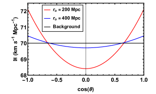
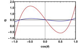
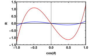
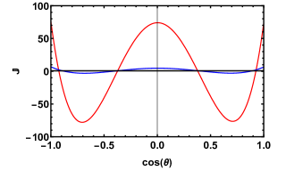
Figure 1: The lowest order covariant cosmographic parameters $\mathbb{H}$, $\mathbb{Q}$, $\mathbb{R}$ and $\mathbb{J}$ at the event of observation are shown as a function of $\cos\theta$, the angular separation from the symmetry axis. The red curves represent local measurements for an observer $200\,$Mpc away from the overdensity, and the blue for an observer at a distance of $400\,$Mpc. The same toy model is assumed, with parameters $H_{0}=70\,$Mpc/km/s, $\delta_{c}=2.5$ and $R_{s}=37.4\,$Mpc.

In FIG. 1 we show the angular dependence of the covariant cosmographic parameters $\mathbb{H},\mathbb{Q},\mathbb{J}$ and $\mathbb{R}$, as functions of $\cos\theta$ for two observers at different distances, $r_{o}=200$ and $400$ Mpc, from the high density peak. We also show, for comparison, the input values of the Hubble, deceleration, jerk and curvature for the smooth background of the toy model (the EdS model), whose value is, by construction, independent of direction. The amplitude of the anisotropies in each parameter becomes weaker as the distance of the observer from the density peak increases. As the observer moves away from the center, the covariant cosmographic parameters asymptotically converge to the background values.

V.2 Luminosity Distance of Toy Model: Linear Perturbation Theory

We can determine the luminosity distance of objects in the single-attractor toy model also through the linear cosmological perturbations. This independent determination, although based on knowledge of the line element (28), and thus model-dependent, provides a useful comparative tool for assessing the validity of the third-order cosmographic expansion (cf. eq. (14)) in the local perturbed Universe.

In a linearly perturbed EdS background, the redshift measured by a matter-comoving observer is Durrer (2021)

$$1+z=(1+z_{c})\big{[}1+\boldsymbol{n}\cdot(\boldsymbol{v}-\boldsymbol{v}_{o})-(\Phi-\Phi_{o})\big{]}\,,$$ (38)

where $z_{c}$ is the background cosmological redshift

$$1+z_{c}=\frac{a_{0}}{a}\,.$$ (39)

For an observer in the matter frame, the luminosity distance to a galaxy with peculiar velocity $\boldsymbol{v}$ is Hui and Greene (2006); Bonvin et al. (2006)

$$d_{L}(z)=d_{L}^{c}(z_{c}(z))\,\big{(}1+2\boldsymbol{n}\cdot\boldsymbol{v}-\boldsymbol{n}\cdot\boldsymbol{v}_{o}\big{)}\,.$$ (40)

Here $\boldsymbol{v}_{o}$ is the velocity of the matter-comoving observer and $d_{L}^{c}(z_{c})$ is the luminosity distance between the events of emission and absorption, assuming that the Universe is perfectly smooth. In the EdS model, this takes the form

$$d_{L}^{c}(z_{c})=\frac{2}{H_{0}}\left(1+z_{c}-\sqrt{1+z_{c}}\right)\,.$$ (41)

Note that the perturbation of the luminosity distance which is induced by the gravitational potential $\Phi$ is not taken into account. Although these provide a first-order correction to the redshift expression (cf. eq. (38), at small redshift ($z\ll 1$), their relative contribution to the distance expression is negligible. Both the redshift and the luminosity distance measured in the CMB frame can be obtained by simply setting $\boldsymbol{v}_{o}=0$.

All the quantities in the preceding expressions ($z_{c}$, $\boldsymbol{v}$, $\Phi$, $\boldsymbol{n}$) depend on the coordinates $(t,r,\psi)$, at which the photon reaching the observer at the event ($t_{0},r_{o},\psi_{o}$) was emitted. We compute them by solving the geodesic equation of the photon in the EdS background for an off-center observer ($r_{o}\neq 0$) as detailed in Appendix (A). This, in turn, allows us to calculate, numerically, the expression for the luminosity distance of the sources as a function of the redshift and the line-of-sight direction and, therefore, the value of $\eta(z,\theta)$.

As a consistency test, we have checked that the cosmographic and the linear perturbation formalisms consistently provide the same expression of the Hubble parameter as measured in the matter frame. The Hubble parameter in a generic spacetime is defined as

$$\mathbb{H}\circeq\frac{\mathrm{d}\,z}{\mathrm{d}\,d}\,.$$ (42)

In Maartens et al. (2023), we demonstrated that when calculated in the matter frame, this relation holds whatever is the operational definition of the distance $d$. Therefore, with $d=d_{L}$ and using eqs. (38) and (40), we obtain with ignoring $\dot{\Phi}$,

$$\mathbb{H} \circeq H\left(1-\boldsymbol{n}\cdot\boldsymbol{v}+\boldsymbol{n}\cdot\frac{\mathrm{d}\boldsymbol{v}}{\mathrm{d}z_{c}}-\frac{\mathrm{d}\Phi}{\mathrm{d}z_{c}}\right)$$ (43)

$$\circeq H\left[1-n^{i}v_{i}+\frac{n^{j}\big{(}-\dot{v}_{j}+n^{i}\partial_{i}v_{j}\big{)}-n^{i}\partial_{i}\Phi}{H_{0}}\right]\,.$$

Since a dust fluid element moves along time-like geodesics, then at ($t_{0},r_{o}$), when the scale factor is $a=1$, its velocity must satisfy the equation of motion

$$\dot{v}_{i}+Hv_{i}\circeq-\partial_{i}\Phi\,.$$ (44)

Once inserted in eq. (43), this allows us to consistently retrieve the formula for the local Hubble parameter given in eq. (35) if we ignore the terms in order $\Phi$. However, the terms containing the gravitational potential could also be found if the contribution of $\Phi$ was also taken into account in the expression of $d_{L}$ (according to the formula C21 in Hui and Greene (2006)). We also note, incidentally, that if the 4-acceleration of the fluid element does not vanish, then the terms which have one $n^{i}$ in eq. (43) will not cancel. As a consequence, the generalized Hubble parameter measured by a matter-comoving observer will display also a dipolar component.

VI Expansion rate fluctuations field of the toy model

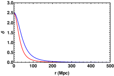
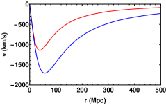
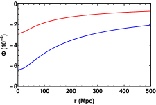
Figure 2: The density contrast, the radial component of the peculiar velocity, and the gravitational potential ($\Phi/c^{2}$), all evaluated at present time, as a function of the radial coordinate $r$ for the $M1$ (red) and $M2$ (blue) models.

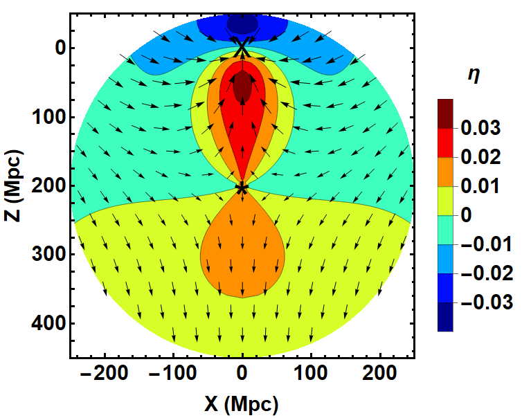
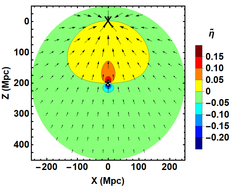
Figure 3: The expansion rate fluctuation field in the matter frame (left) and in the CMB frame (right) for the model $M1$ is portrayed in the $(X,Z)$-plane containing the axis between the center of the mass overdensity, at $(X,Z)=(0,0)$, and the observer, at (0,200). Arrows display the peculiar velocity (vector) field, while color maps and isocontours display the amplitude of the expansion rate fluctuation (scalar) field.

As well as serving as a test bed for the limits of the cosmographic approach in the local Universe, the toy model is designed to roughly reproduce the expansion rate fluctuations measured with real data by Kalbouneh et al. (2023), thus enabling a better understanding of their physical origin. It also allows us to compare and contrast the structure and characteristics of the expansion rate fluctuation field, measured in two different reference systems, the matter-comoving and the CMB frames.

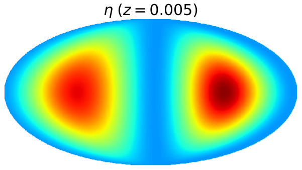
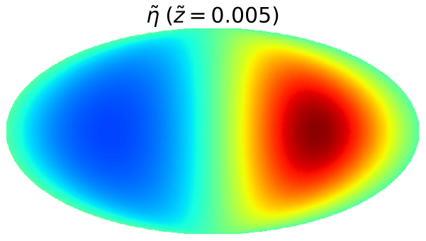
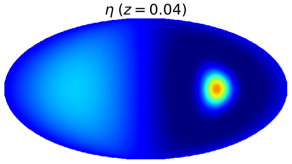
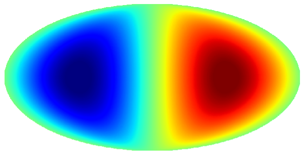
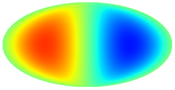
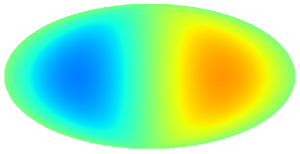
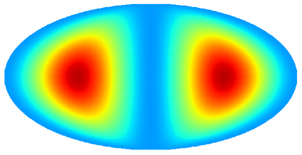
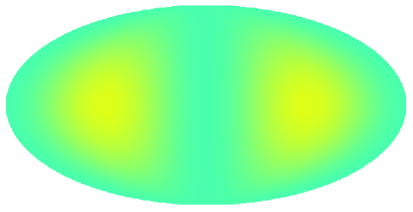
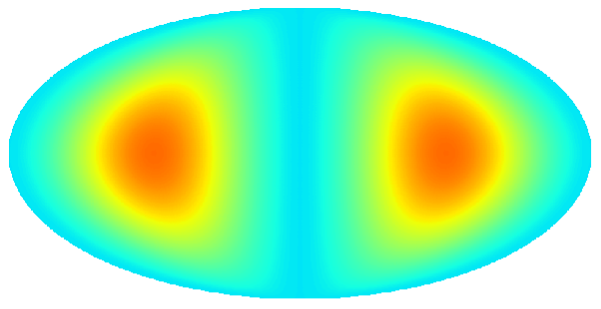
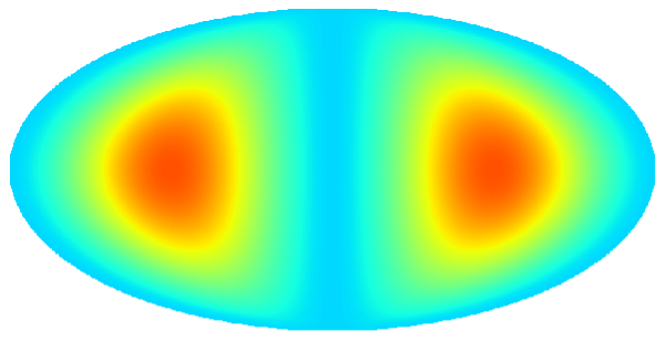
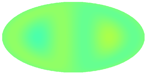
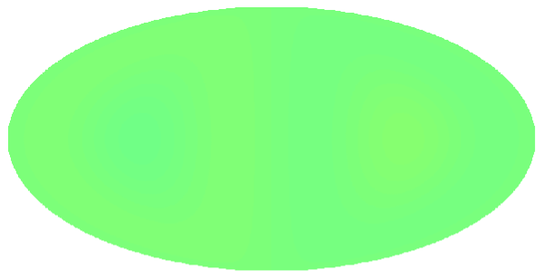
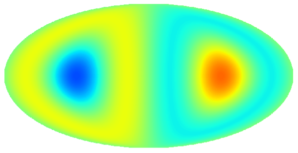
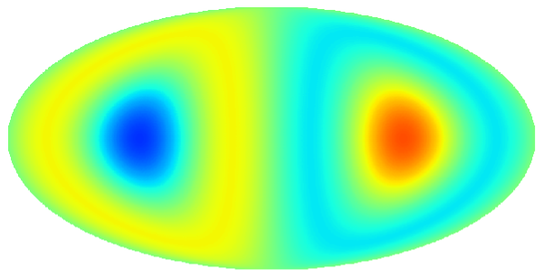
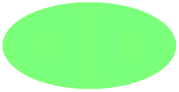
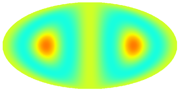
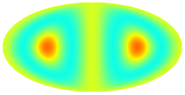
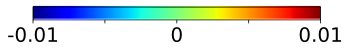
Figure 4: All-sky maps of the expansion rate fluctuations field generated by the $M1$ model in matter and CMB frames, at two redshifts (first row, 4 columns). The rows show the multipolar components: dipole (row 2), quadrupole (row 3), octupole (row 4), and hexadecapole (row 5). The first and second columns show $\eta$ (matter frame) and $\tilde{\eta}$ (CMB frame) at $z=0.005$. Columns 3 and 4 show the same fields at a deeper redshift ($z=0.04$). The position of the overdense region is chosen to lie on the equator of the Mollweide projection, $90^{\circ}$ away from the center.

We set the parameters of the toy model so as to describe two competing and antagonistic scenarios often invoked to explain the kinematics of the local Universe within the standard model of cosmology. One model (hereafter $M1$) has a peculiar velocity field which is sourced by a relatively local mass overdensity and thus results in a bulk motion which vanishes on small averaging scales. In the opposite scenario, dubbed $M2$, the attractor mass is larger and further away from the observer, thus a coherent bulk motion signal is still present in a large volume with typical size $R\sim 500$Mpc.

The small-scale bulk model $M1$ is given by using

$$M1:\quad r_{o}=200\,{\rm Mpc}\,,\leavevmode\nobreak\ \leavevmode\nobreak\ \delta_{c}=2.5\,,\leavevmode\nobreak\ \leavevmode\nobreak\ R_{s}=37.4\,{\rm Mpc}\,,$$ (45)

in eq. (30). This choice implies $\Phi_{c}=-2.9\times 10^{-4}$. These values are suggested by studies of the peculiar velocity field in the local Universe Marinoni et al. (1998) and fairly characterize the scenario in which such a field is generated by a single attractor like the Shapley supercluster. The values we choose for the parameters $\delta_{c}$ and $R_{s}$ are consistent with Marinoni et al. (1998), but they are fixed so that the observer (here assumed to be 200 Mpc far from Shapley) moves relative to the CMB with a velocity of $320$ km/s. This value is the component of our Local Group which is generated by a matter distribution at distance $>38\,$Mpc, as measured by Tully et al. (2019). The large-scale bulk model $M2$ is given by

$$M2:\quad r_{o}=400\,{\rm Mpc}\,,\leavevmode\nobreak\ \leavevmode\nobreak\ \delta_{c}=2.5\,,\leavevmode\nobreak\ \leavevmode\nobreak\ R_{s}=56\,{\rm Mpc}\,,$$ (46)

which generates the same observer’s velocity ($\sim 320$ km/s).

The background EdS geometry is common to the two models, with $H_{0}=70$ $\mathrm{km\;s^{-1}Mpc^{-1}}$, $q_{0}=0.5$, $\Omega_{k0}=0$, and $j_{0}=1$. In FIG. 2, the density contrast, the radial component of the velocity profile today, and the gravitational potential for these two scenarios are shown as a function of the radial coordinate $r$.

In FIG. 3 we display a planar section of the $M1$ toy model of the Universe. This plane contains the center of the Shapley overdensity contrast and the observer, at a distance of 200 Mpc. We also show, superimposed, the peculiar velocity (vector) field generated by the mass overdensity as well as the isocontours of the expansion rate fluctuation (scalar) field. Both fields show different configurations, depending on whether they are measured in the matter or CMB frames respectively.

Regardless of the observer, a common feature that emerges from visual inspection is the characteristic anisotropic structure of the expansion rate fluctuations field induced by metric perturbations. In addition, when looking along a fixed direction of the observer’s line of sight, one can also visually appreciate the nonlinearities in the distance-redshift relationships, which are most evident in the direction of the supercluster.

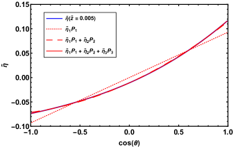
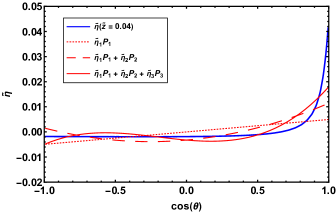
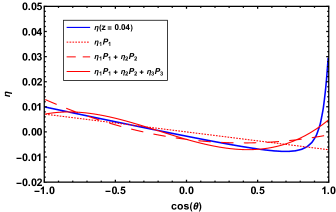
Figure 5: The expansion rate fluctuation field of the $M1$ model in the CMB frame (upper panels) and matter frame (lower panels), shown as a function of $\cos\theta$ at redshift $z=0.005$ (left panels) and $z=0.04$ (right panels). We also show how the signal is reconstructed by different order Legendre expansions, up to $\ell=3$.

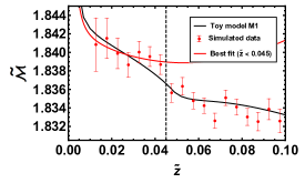
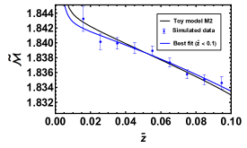
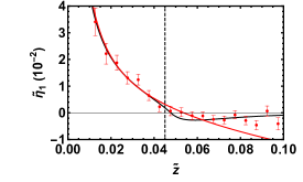
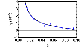
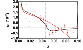
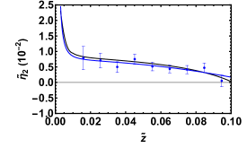
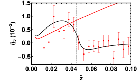
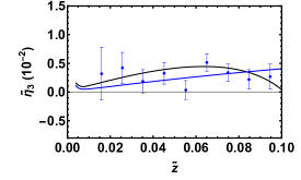
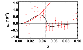
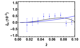
Figure 6: Left panels: The normalization $\mathcal{M}$, dipole, quadrupole and octupole of the expansion rate fluctuation field in the CMB frame ($\tilde{\eta}_{\ell}$), reconstructed using $M1$ simulated galaxy data in different redshift shells (red points). These are compared to the input continuous value (black solid line) and to the best-fitting theoretical predictions (red curves). The latter are obtained by expanding $\tilde{\eta}$ using the cosmographic approach, truncated up to $\mathcal{O}(z^{3})$, and by fitting only the points with $\tilde{z}<0.045$. Right panels: as on the left, but for the $M2$ simulated data (blue points). The best theoretical models (blue curves) are obtained by fitting all the available measurements up to $z=0.1$.

The scalar nature of the $\eta$ observable allows the multipolar structure of the signal to be captured even if only visually. At low redshift (close to the observer), the amplitude of $\eta$ measured in the matter frame is dominated by a quadrupolar component, while that inferred in the CMB frame shows a typical dipolar pattern. The fact that, by definition, the velocity field vanishes around the matter-comoving observer (see left panel of FIG. 3), means that the fluctuations of the expansion velocity field are dominated by a shear component. In other words, the expansion rate is similarly perturbed in antipodal directions around the observer. When the distance increases, the peculiar velocity field reveals more complex characteristics. As a consequence, the expansion rate fluctuation field also acquires non-trivial distortions. In the CMB frame (right panel of FIG. 3), the expansion rate field is locally dominated by a dipolar component, induced by the motion of the observer relative to the chosen reference frame. Its amplitude increases closer to the observer.

A quantitative estimation of the multipolar components of $\eta$ for $M1$ is presented in FIG. 4, where we show the multipoles of the expansion rate fluctuation measured by the matter-comoving and CMB-comoving observers. The multipole decomposition is shown at two characteristic redshifts, $z=0.005$ – assumed to represent very local measurements, and $z=0.04$ – representing regions where the peak density of the toy model severely distorts the distance-redshift relationship. The nonzero value of a multipole provides information on the structure of the anisotropy in the expansion rate, while its evolution with redshift reflects the level of nonlinearity in the distance-redshift relation. The qualitative similarity with the signal extracted by Kalbouneh et al. (2023) (in the CMB frame) from Cosmicflows-3 and Pantheon samples is apparent: the axes of the multipoles are aligned, the geometry is axisymmetrical, and the amplitude and redshift scaling of each multipole roughly reproduce what was observed by Kalbouneh et al. (2023) (compare their FIG. 4).

The expansion rate fluctuations in the CMB frame are enhanced relative to the signal measured by the matter-frame observer. This increase is essentially contributed by the dipolar component, which, as expected on the basis of eq. (27), is the multipole that is most sensitive to observer velocity effects. Furthermore, as eq. (17) makes clear, the smaller the volume surrounding the observer in which the dipole signal is estimated, the greater the increase in the signal. On the contrary, in the same limit $z\rightarrow 0$, the dipole of $\eta$ in the matter frame is expected to vanish (cf. eq. (22)), as shown in FIG. 4. The distortions induced by the motion of the observer in the dipole are of order $v_{o}/\tilde{z}$. As one pushes the analysis to higher $\tilde{z}$, the amplitude of $\tilde{\eta}_{1}$ is suppressed inversely proportional to redshift. Consequently, the signal becomes more sensitive to metric contributions, particularly to the dipole of the deceleration parameter, $\mathbb{Q}_{1}$. The increasingly important effects induced by $\mathbb{Q}_{1}$ can be seen by comparing the low- and high-redshift dipolar components measured in the matter frame.

Visual inspection of FIG. 4 shows that the relative motion of the CMB and matter observers only affects the dipole of $\tilde{\eta}$, while minimally affecting its quadrupole and octupole. In fact, already at very low redshift, the contribution of velocity-induced distortions to the signal is ${\cal O}(v_{o}^{2}/z^{2})$ and ${\cal O}(v_{o}^{3}/z^{3})$ respectively. Note that, contrary to the case of other multipoles, $\eta_{2}$ does not vanish for $z\rightarrow 0$, but in this limit becomes proportional to the amplitude of the quadrupole $\mathbb{H}_{2}$.

Similarly to the case of the dipole, as redshift increases, the differences between the reconstructed multipoles of $\eta$ in the matter and CMB frames, are reduced and the signal acquires specific dependencies on the higher-order multipoles of the covariant cosmographic parameters. FIG. 4 shows that the quadrupole signal $\eta_{2}$ in the $M1$ toy model weakens with redshift, because the quadrupole contributions of $\mathbb{Q}$ and $\mathbb{J}-\mathbb{R}$ – which are negative in this model (see TABLE 1) – gradually become more important. The same applies to the octupole and the hexadecapole signals $\eta_{3}$ and $\eta_{4}$, whose low-$z$ amplitude becomes progressively more sensitive to a mixture of multipoles of higher-order cosmographic parameters. Although these are only ${\cal O}(z^{2})$ corrections, large values of the covariant cosmographic parameters, as indeed is the case if the metric has large fluctuations (see TABLE 1), compensate for the suppression induced by the powers of small $z$.

In FIG. 5 we show how well the expansion rate fluctuations in the CMB and matter frames are reconstructed by the lower multipoles, at redshifts $z=0.005$ and $z=0.04$. As expected, a multipolar expansion up to $\ell=2$ is enough to achieve percentage estimation precision at low redshift. However, the higher the redshift, the more inaccurate the estimation is. Note that, given the different functional shapes of the expansion rate fluctuations in different observer frames, at an equal order of expansion, the Legendre approximation in the matter frame has a somewhat higher level of precision than in the CMB frame, with the accuracy increasing by roughly $5\%$.

VII Forecasting Precision on Cosmographic Parameters estimation

Model	Small-Scale Bulk ($M1$) ($\delta_{c}=2.5,R_{s}=37.4$ Mpc, $r_{o}=200$ Mpc)					Large-Scale Bulk ($M2$) ($\delta_{c}=2.5,R_{s}=56$ Mpc, $r_{o}=400$ Mpc)
$X$	$X_{0}$	$X_{1}$	$X_{2}$	$X_{3}$	$X_{4}$	$X_{0}$	$X_{1}$	$X_{2}$	$X_{3}$	$X_{4}$
$\mathbb{H}$ (km/s/Mpc)	$69.65$	-	$2.47$	-	-	$69.86$	-	$1.29$	-	-
$\mathbb{Q}$	$0.51$	$-0.58$	$-0.09$	$1.88$	0	$0.505$	$-0.125$	$-0.05$	$0.51$	0
$\mathbb{J}-\mathbb{R}$	$-6.53$	$1.16$	$-57.3$	$-3.76$	$138.5$	$0.17$	$0.25$	$-6.37$	$-1.02$	$19.3$
$v_{o}$ (km/s)	$320$					$320$
Best fitting values
$X$	$X_{0}$	$X_{1}$	$X_{2}$	$X_{3}$	$X_{4}$	$X_{0}$	$X_{1}$	$X_{2}$	$X_{3}$	$X_{4}$
$\mathbb{H}$ (km/s/Mpc)	$69.5\pm 1.0$	-	$2.1\pm 0.5$	-	-	$69.63\pm 0.30$	-	$1.1\pm 0.2$	-	-
$\mathbb{Q}$	$0.4\pm 2.0$	$-0.9\pm 0.3$	$0$	$0.9\pm 0.2$	0	$0.7\pm 0.3$	$-0.18\pm 0.05$	$0$	$0.23\pm 0.05$	0
$\mathbb{J}-\mathbb{R}$	$16\pm 87$	$0$	$-42\pm 32$	$0$	$73\pm 16$	$-2.3\pm 5.9$	$0$	$-7.4\pm 3.1$	$0$	$6.8\pm 1.9$
$v_{o}$ (km/s)	$336\pm 32$					$303\pm 20$

Table 1: The upper table shows the Legendre multipoles $X_{\ell}$ ($\ell\leq 4$) of the covariant cosmographic parameters and the relative velocity $v_{o}$ between the matter and the CMB frames for the $M1$ (left) and $M2$ (right) toy models. These quantities are calculated using the equations presented in Appendix B. The lower table shows the best-fit values (and the $68\%$ confidence interval) deduced from the likelihood analysis performed using $15,000$ discrete objects sampling the toy models and roughly reproducing the ZTF survey characteristics. A cell containing a dash indicates that the multipole vanishes by definition. A cell containing a zero means that the multipole is intrinsically small and its value is therefore set to zero by default. Note that for $\ell>0$, $\mathbb{J}_{\ell}-\mathbb{R}_{l}\approx\mathbb{J}_{l}$.

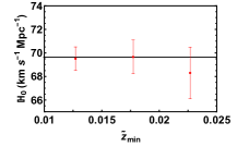
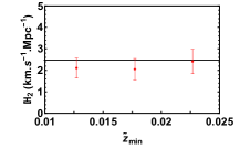
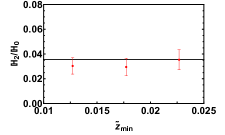
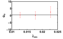
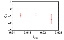
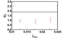
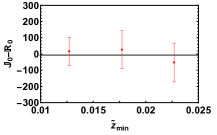
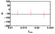
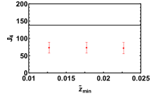
Figure 7: The best-fitting values (and the associated $1\sigma$ errorbars) for the covariant cosmographic parameters extracted from the analysis of the $M1$ simulation in the shell $\tilde{z}_{\rm min}<\tilde{z}<0.045$, are shown as a function of $\tilde{z}_{\rm min}$. The black lines show, for comparison, the true simulated input values (see TABLE 1).

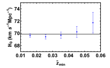
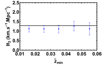
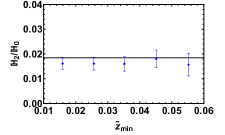
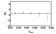
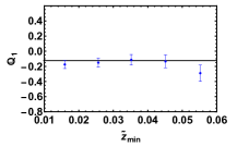
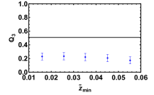
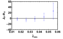
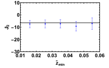
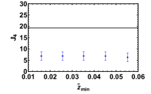
Figure 8: As in FIG. 7, but for the $M2$ simulation. The best-fitting parameters recovered in the shell $\tilde{z}_{\rm min}<\tilde{z}<0.1$ are shown as a function of $\tilde{z}_{\rm min}$.

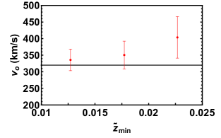
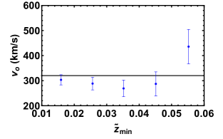
Figure 9: The best-fitting velocity (and the associated $1\sigma$ errorbar) of the matter frame relative to the CMB frame at the event of observation. Left: results from the analysis of the $M1$ simulation in shells $\tilde{z}_{\rm min}<\tilde{z}<0.045$. Right: results from the analysis of the $M2$ simulation in shells $\tilde{z}_{\rm min}<\tilde{z}<0.1$.

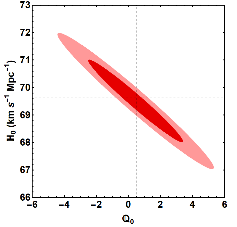
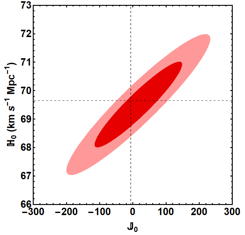
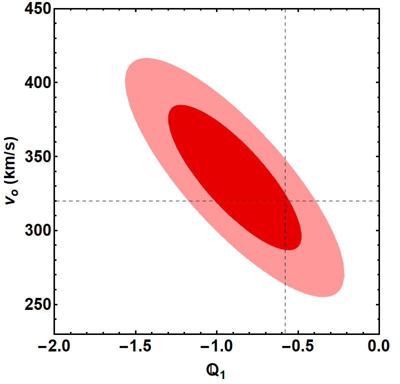
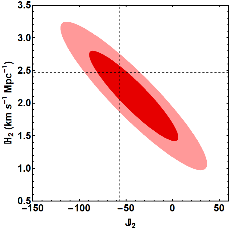
Figure 10: The $68\%$ and $95\%$ confidence level contours in various 2D parameter spaces obtained from the likelihood analysis of the $M1$ simulated data ($\tilde{z}<0.045$). The intersection of the two dashed lines indicates the input value.

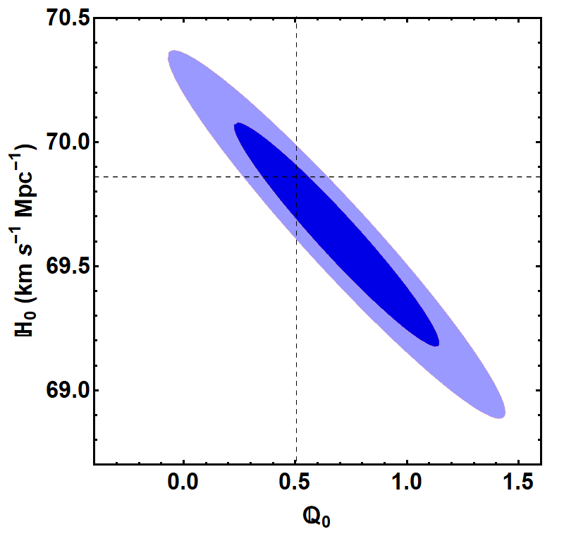
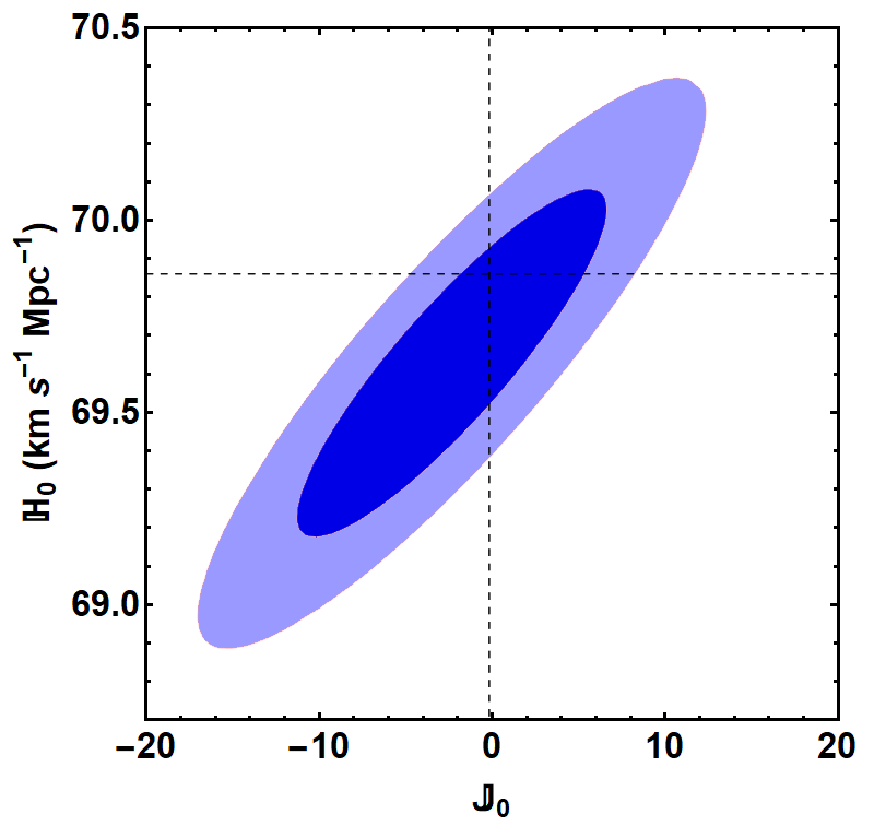
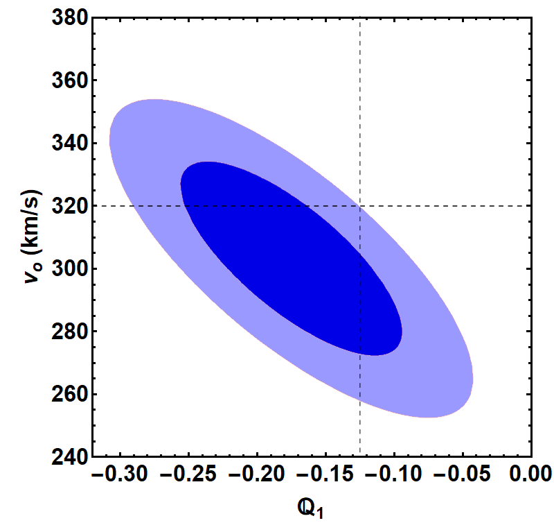
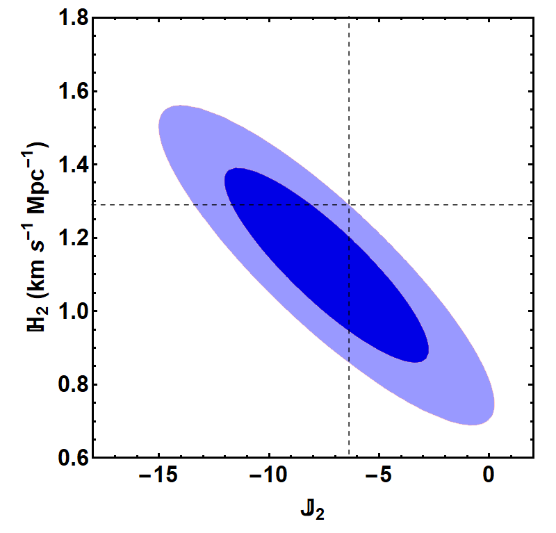
Figure 11: The $68\%$ and $95\%$ confidence level contours in various 2D parameter spaces obtained from the likelihood analysis of the $M2$ simulated data ($\tilde{z}<0.1$). The intersection of the two dashed lines indicates the input value.

By means of the toy models, we can also assess the accuracy with which the (idealized) continuous $\eta$ field is reconstructed using a (real) discrete point process, and forecast the precision with which future data sets will constrain multipoles of the covariant cosmographic parameters in the local Universe ($z\lesssim 0.1)$.

To this end, we simulate distances and redshifts for $15\times 10^{3}$ galaxies, distributed in the redshift interval $0.01<\tilde{z}<0.1$, by sampling the continuous toy models $M1$ and $M2$ according to the redshift distribution expected from the ZTF survey Amenouche (2022). In order to make these two simulated catalogs of distances (measured without using redshift information) as realistic as possible, we assume that the distance modulus of each object has a Gaussian distribution with standard deviation $\sigma_{\mu}=0.15$ Dhawan et al. (2022b), and no correlation between the measurements.

We measure the expansion rate fluctuations (in the CMB frame) in spherical shells $S$ of thickness $\delta\tilde{z}=0.005$ for the $M1$ model and $\delta\tilde{z}=0.01$ for $M2$ model. In FIG. 6, the amplitude of the multipoles $\tilde{\eta}_{\ell}$, inferred using the discrete catalogs $M1$ and $M2$, is compared to the input theoretical value characterizing the continuous matter density fields. The estimation is unbiased and its accuracy, for both the small- and large-scale bulk scenarios, is remarkable. However, extracting the value of covariant cosmographic parameters from these measurements is challenging.

As shown by Heinesen (2021), the covariant cosmographic parameters $\mathbb{H},\mathbb{Q}$, $\mathbb{J}$ and $\mathbb{R}$ introduce 58 degrees of freedom (if the 4-acceleration is zero) in the analysis. By fitting all independent multipoles to the data simultaneously, one is faced with statistical degenerations that prevent accurate parameter determination Dhawan et al. (2022a); Cowell et al. (2023). Additional arguments, based on the symmetries of the expansion velocity field, help circumvent this problem. We start by recognizing the axisymmetric configurations for the expansion rate fluctuations, through the analysis of the multipolar structure of the $\eta$ signal. Then we neglect terms of order ${\cal O}[(\mathbb{H}_{2}/\mathbb{H}_{0})^{2}]$ and ${\cal O}(z^{3})$. Consequently, the fitting parameters are consistently reduced down to a total of 12: 2 d.o.f. related to $\mathbb{H}$, 4 to $\mathbb{Q}$ and 6 to $\mathbb{J}-\mathbb{R}$. A second major simplification is induced by the fact that some multipoles of the covariant cosmographic parameters (cf. equations (6,7,8)), contain spatial gradients, as shown by Heinesen and Macpherson (2022). The magnitude of those multipoles is thus increased by factors inversely proportional to the typical spatial scales of the inhomogeneities. For example, we show in Appendix B that the odd multipoles of $\mathbb{Q},\mathbb{R}$ and $\mathbb{J}$, containing a spatial derivative, are proportional to $1/\xi_{H}$ (with $\xi_{H}\ll 1$) while the monopole, the quadrupole and the hexadecapole of $\mathbb{J}$, containing a second order spatial derivative, scale as $1/\xi_{H}^{2}$. Because of this only terms containing powers of $(z/\xi_{H})$ contributes significantly in the expansions (21,22,23,24,25). This very same argument also allows to resolve the degeneracy between $\mathbb{J}$ and $\mathbb{R}$ appearing when truncating the expansion of $\eta$ at order $\mathcal{O}(z^{3})$: the contribution of the latter parameter being always much smaller with respect to that of the former, is always negligible for all $\ell\geq 1$ (in principle we never discard the monopoles since we expect to recover the FLRW cosmographic parameters in the limit of small expansion rate perturbations). Summing up, on top of all the monopoles, we only consider, in the fitting scheme, the dominant multiples $\ell\geq 1$. We can therefore further reduce the total number of free-fitting parameters to 9. Note that the velocity $v_{o}$ of the matter frame relative to the CMB frame is also counted in this number.

The optimal analysis scheme therefore consists in decomposing $\tilde{\eta}$ measured in the CMB frame into spherical harmonics, then comparing each multipole with theoretical predictions via a likelihood analysis in order to constrain the free parameters of the model, $\boldsymbol{X}=\big{(}v_{o},\mathbb{H}_{0},\mathbb{H}_{2},\mathbb{Q}_{0},\mathbb{Q}_{1},\mathbb{Q}_{3},\mathbb{J}_{0}-\mathbb{R}_{0},\mathbb{J}_{2},\mathbb{J}_{4}\big{)}$. This is achieved in practice by minimizing the $\chi^{2}$ statistic

$$\chi^{2}(\boldsymbol{X})=\sum_{i=1}^{N_{\rm sh}}\left[\frac{\tilde{\mathcal{M}}(\boldsymbol{X},\tilde{z}_{i})-\tilde{\mathcal{M}}_{i}}{\sigma_{\tilde{\mathcal{M}}_{i}}}\right]^{2}+\sum_{\ell=1}^{\ell_{\rm max}}\sum_{i=1}^{N_{\rm sh}}\left[\frac{\tilde{\eta}_{\ell}(\boldsymbol{X},\tilde{z}_{i})-(\tilde{\eta}_{\ell})_{i}}{\sigma_{(\tilde{\eta}_{\ell})_{i}}}\right]^{2},$$ (47)

where $N_{\rm sh}$ is the number of redshift shells, indexed by $i$, while $\ell$ labels each multipole ($\ell_{\rm max}=4$). The theoretical models for $\tilde{\mathcal{M}}$ and $\tilde{\eta}_{\ell}$ are obtained by combining equations (21), (22), (23), (24) and (25) with equations (27) – and by setting $\mathbb{Q}_{2}=\mathbb{J}_{1}-\mathbb{R}_{1}=\mathbb{J}_{3}-\mathbb{R}_{3}=0$, as discussed above. The method for estimating the multipoles $\tilde{\mathcal{M}}_{i}$ and $(\tilde{\eta}_{\ell})_{i}$, and their uncertainties in each shell $i$, is detailed in Appendix C: see eqs. (80) and (81).

The accuracy of this inference scheme is tested using the catalogs $M1$ and $M2$. In FIG. 6 (left panels), we show the result of fitting the redshift evolution of the lowest multipoles of $\tilde{\eta}$, together with the normalizing factor $\mathcal{\tilde{M}}$, by means of the $M1$ dataset. FIG. 6 (right panels) presents similar results obtained from the analysis of the $M2$ catalog. In TABLE 1, we quote the best-fitting values of the covariant cosmographic parameters and compare them to the true input values, for both models $M1$ and $M2$.

FIG. 6 shows how well the discrete objects simulating the ZTF survey trace the underlying continuous (exact) field and how well the multipoles of $\eta$ are reconstructed using the expansion in covariant cosmographic parameters – i.e., by neglecting $\mathcal{O}(z^{3})$ terms in eqs. (21), (22), (23), (24) and $(\ref{hexe})$. For the toy model $M1$, we see that the goodness of the fit is satisfactory at low redshift, but breaks down at $z\approx 0.045$. This value is not an insignificant one: it is approximately the distance of the large density peak simulated in the toy model $M1$, the scale at which strong nonlinearities in the distance-redshift relationship emerge. The causes of these nonlinear effects and their effect on cosmographic reconstruction are discussed in detail in the next section. We observe that the existence and value of this break-down scale can be easily recognized from the data, without any prior knowledge of the magnitude and size of matter fluctuations in the local Universe.

In the case of the large-scale bulk model $M2$, where the attractor lies on the edge of the region covered by the simulated data ($0.01<\tilde{z}<0.1$), the cosmographic expansion is even more effective, describing the evolution of the signal over the entire redshift interval analyzed. As a consequence, the value of the $\chi^{2}$ statistic becomes highly significant. We find $\chi^{2}=49.2$ for $9\times 5-9=36$ degrees of freedom, implying that the probability of finding a higher $\chi^{2}$ value is around $7\%$.

In FIGS. 7 and 8 we display the best-fitting values for the lowest multipoles of the covariant cosmographic parameters $\mathbb{H}$ (monopole and quadrupole), $\mathbb{Q}$ (monopole, dipole, and octupole), and $\mathbb{J}-\mathbb{R}$ (monopole, quadrupole, and hexadecapole). We also show how well these estimates approximate the simulated input values. Note that the cosmographic parameters characterize the structure of spacetime at the position of the observer. However, it is not feasible to constrain their amplitude using measurements of $\eta$ at $z=0$. Their value is extrapolated from $\eta$ measurements made in spherical shells centered on the observer and with variable width. The upper boundary is fixed at the maximum redshift (at which the fit is not rejected by the $\chi^{2}$ test), while the lower boundary of the shell, $\tilde{z}_{\rm min}$, is left free to vary. The smaller $\tilde{z}_{\rm min}$ becomes, the more data are used in the likelihood analysis, and the closer the best-fitting parameter is to the actual value simulated at $z=0$. As a matter of fact, virtually all the estimates of the cosmographic parameters converge to the simulated values as $\tilde{z}_{\rm min}\to 0$. The statistical uncertainties of the reconstructed parameters decrease as the volume in which the expansion rate fluctuation is calculated grows larger. Note however that estimates for different values of $\tilde{z}_{\rm min}$ are correlated, given the cumulative nature of the binning strategy.

It is important that the likelihood analysis is performed also by fitting the normalization factor $\mathcal{M}$. This quantity could be biased in principle because it contains information on the zero-point calibration of brightness distances. It is also sensitive to possible systematic, distance-dependent errors in the estimation of the distance modulus. If, for conservative reasons, we exclude the $\mathcal{M}$ function from the likelihood analysis, we cannot any more provide an independent estimate of the amplitudes of the monopole and quadrupole of the generalized Hubble parameter $\mathbb{H}$. Only the ratio $\mathbb{H}_{2}/\mathbb{H}_{0}$ (shown in the upper right plots in FIG. 7 and 8) can be constrained in this case. By contrast, the accuracy in estimating the multipoles (with $\ell>0$) of $\mathbb{Q}$ and $\mathbb{J}$ is not affected by the analysis strategy. As a consequence, any systematic miscalibration of the normalization of galaxy distances will not have any impact in the reconstruction of the multipoles of $\mathbb{Q}$ and $\mathbb{J}$.

As shown in TABLE 1 and also in FIGS. 7 and 8, the only parameters that are mis-recovered (for $M1$ or $M2$) are $\mathbb{Q}_{3}$ and $\mathbb{J}_{4}$. As a consequence of the subdominance of certain multipoles, the only term that contributes to the amplitude of $\eta_{3}$ (cf. eq. (24)) is the linear one (i.e. $\mathbb{Q}_{3}$), while the amplitude of $\eta_{4}$ is effectively determined only by $\mathbb{J}_{4}$ (cf. eq. (25)). Therefore, the theoretical form of the octupole and hexadecapole of the expansion rate fluctuation field is controlled by only one monomial of the redshift, which is a severe limitation in the ability to reproduce the observed redshift evolution of the data. The optimal way to tackle this issue is to include in the analysis the fourth and fifth derivatives of distance (snap and crackle) in the expansion (3). Here, instead, we simply parametrize our ignorance by means of two nuisance parameters $\mathbb{A}$ and $\mathbb{B}$ over which we subsequently marginalize in the statistical analysis. Although in this way we overall increase the statistical uncertainty in the best fitting parameters $\mathbb{Q}_{3}$ and $\mathbb{J}_{4}$, we significantly reduce the systematic error. We thus add, in accordance to an educated guess about the symmetry of the problem, a term $\mathbb{A}\,z^{3}$ to eq. (24) and a term $\mathbb{B}\,z^{4}$ to eq. (25) and re-do the likelihood analysis. For $M1$, we obtain $\mathbb{Q}_{3}=1.0\pm 0.6$ and $\mathbb{J}_{4}=94\pm 69$. As expected the discrepancy between the recovered octupole of $\mathbb{Q}$ and its simulated value decreased from $4.9\sigma$ to $1.5\sigma$. As for the hexadecapole of $\mathbb{J}$, the deviation from the expectation reduces from $4.1\sigma$ to $0.7\sigma$ (the best fitting values for nuisance parameters are $\mathbb{A}=-19\pm 89$ and $\mathbb{B}=(-1\pm 3)\times 10^{3}$ respectively. For $M2$, the new analysis returns $\mathbb{Q}_{3}=0.36\pm 0.13$ and $\mathbb{J}_{4}=32\pm 7$ and the tension decreases from $5.6\sigma$ to $1.2\sigma$, and from $6.6\sigma$ to $1.8\sigma$, respectively (the best fitting values for nuisance parameters are $\mathbb{A}=-4\pm 4$ and $\mathbb{B}=-276\pm 71$ respectively.

The velocity $v_{o}=320$ km/s of the matter relative to the CMB is reconstructed quite well from the analysis of both simulated catalogs $M1$ and $M2$. FIG. 9 shows that the relative error of the best-fitting velocity is about $10\%$ and $7\%$ for the $M1$ and $M2$ scenarios respectively. The same caveat as before applies. If $v_{o}$ is inferred from the analysis of $\tilde{\eta}$ reconstructed in shells at large distance from the observer, the estimation is affected by large uncertainties. However, as soon as the lower boundary $\tilde{z}_{\rm min}$ of the shell in which $\tilde{\eta}$ is reconstructed approaches zero, the estimates of the local covariant cosmographic parameters stabilize and in the limit converge to the input simulated values.

Parameter estimation is clearly affected by statistical degeneracies. These are visible in FIGS. 10 and 11 which show the 2-dimensional $68\%$ and $95\%$ likelihood contours of relevant cosmographic parameters. The analysis of $M1$ and $M2$ suggests that the accuracy of statistical inference depends critically on the structure of the expansion rate fluctuations, rather than on the quality and precision of the distance measurements. The higher the redshift at which the cosmographic expansion breaks down, i.e., the wider the redshift interval in which the amplitude of $\eta$ can be approximated in a model-independent way by an expansion in powers of $z$, the smaller the uncertainties in the recovered cosmographic parameters. The smoother and more spread over a large volume are the perturbations in the local expansion rate (model $M2$), the better the precision of the recovered parameters will be – compared to the case where large perturbations are close to the observer’s position (model $M1$).

Nevertheless, even in the latter ‘pessimistic scenario’, data from a future survey like the ZTF are sufficient to constrain the relevant covariant cosmographic parameters with a fair degree of precision. The parameters that one expects to better reconstruct are the local value of the monopole of the covariant Hubble parameter $\mathbb{H}_{0}$ (with an optimistic/ pessimistic resolution of $0.3/1.0$ km s^-1 Mpc^-1), the quadrupole of $\mathbb{H}$ ($\sim 4\sigma$ detection in the pessimistic scenario, i.e., a relative uncertainty of $24\%$), and the dipole in $\mathbb{Q}$, which is recovered with nearly a $33\%$ precision under the most conservative assumptions.

The degree of reliability of the predictions depends strictly on the degree of realism of the toy model. The constraints on the multipoles of the covariant cosmographic parameters could deviate from expectations even if the specific parameters of future surveys were significantly different from those simplistically assumed in this study. Nevertheless, the results obtained are encouraging and suggest the possibility of obtaining fairly precise estimates of the covariant cosmographic parameters at scales $(z\lesssim 0.1)$ where the CP ceases to be applicable, and of characterising the expansion rate of the local universe in a more meaningful and complete way than is possible using the $H_{0}$ parameter of the Standard Model alone.

VIII Limits of the Cosmographic Expansion

The luminosity distance $d_{L}$ to a source at redshift $z$ depends on the direction of the line of sight, whether calculated in a model-independent cosmographic approach or in a linearly perturbed FLRW model. In FIG. 12 we display its redshift scaling in the direction of the center of the mass overdensity ($\theta=0$), and the opposite direction ($\theta=\pi$), for the matter- and CMB-comoving observers, at a distance of $r_{o}=200\,$Mpc from the density peak of the $M1$ model.

The luminosity distance shows a characteristic elongated $S$-shaped trend along the observer’s line of sight, bending approximately at the position of the density peak. This feature is induced by the radial component of the peculiar velocity of the emitters – which increases/ decreases relative to the background cosmological value for the observed redshift of a source placed before/ after the density peak. If the density peak is sufficiently large (not far from our $\delta_{c}$), the luminosity distance becomes a multivariate function of $z$, and the validity of the cosmographic expansion breaks down. Even before reaching this pathological configuration, the more nonlinear the density field, the poorer becomes the reconstruction of the distance using only lower-order expansion terms.

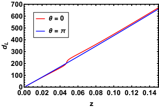
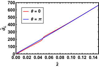
Figure 12: Luminosity distance in the $M1$ toy model, calculated using linear perturbation theory for a matter-comoving observer (left) and a CMB-comoving observer (right). The scaling with redshift along two different line-of-sight directions is shown: towards the center of the density peak ($\theta=0$, solid red line) and in the antipodal direction ($\theta=\pi$, solid blue line).

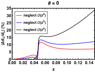
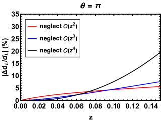
Figure 13: The relative discrepancy between different orders of expansion of the luminosity distance (measured by a matter comoving observer) and the true input value (model $M1$), in the direction of the centre of the density peak (left) and in the opposite direction (right).

FIG. 13 compares the luminosity distance reconstructed using the cosmographic approach against that reconstructed using linear perturbation theory. The relative discrepancy is shown along two line-of-sight directions ($\theta=0$ and $\theta=\pi$) and for different expansion orders in redshift.

The cosmographic expansion of $d_{L}$, eq. (3), works extremely well locally, around the observer, and along any line of sight. It improves the higher the order of expansion is. However, already at relatively low redshifts, $z\approx 0.05$ in the case of the $M1$ model, its accuracy is severely limited if the field is dominated by a nearby large density peak. In this configuration, the luminosity distance deviates considerably from linearity and the cosmographic parameters acquire a large amplitude to allow an accurate description of these distortions in regimes where $z\ll 1$.

In fact, a truncated polynomial expansion at a low order is ineffective in capturing these nonlinear features. It is therefore essential to know at what scales the covariant cosmographic expansion fails if it is to be successfully applied in the highly irregular regions of the local Universe. As expected, if the gravitational source is located far from the observer, as in the case of the $M2$ toy model, the redshift range in which cosmography can be safely applied increases accordingly. The combined analysis of the independent multipoles of $\eta$, as explained in the previous section, makes it easy to identify the scale at which the covariant cosmographic approach breaks down.

IX Multipoles of the radial peculiar velocity field

After showing how to recover model-independent information about the spacetime surrounding the observer, we move on to interpret $\tilde{\eta}$ anisotropies in a more conventional framework, as small deviations from the FLRW metric. In this scenario, fluctuations in $\tilde{\eta}$, instead of providing information on the covariant cosmographic parameters, simply give an insight into the amplitude and distribution of the radial peculiar velocity field, $v_{n}\equiv\boldsymbol{v}\cdot\boldsymbol{n}$, of galaxies relative to an idealized matter frame – which coincides with the CMB frame in perturbed FLRW. If we ignore the gravitational potential in the perturbed FLRW model, we have $\tilde{z}=z_{c}+v_{n}(1+z_{c})$ and $\tilde{d}_{L}=d_{L}^{c}(1+2v_{n})$. As a consequence, we can express $\tilde{\eta}$ as

$$\tilde{\eta}=\log\left[\frac{z_{c}+v_{n}(1+z_{c})}{d_{L}^{c}(1+2v_{n})}\right]-\tilde{\mathcal{M}}=\log\left(\frac{z_{c}}{d_{L}^{c}}\right)-\tilde{\mathcal{M}}+\log\left[1+\frac{v_{n}}{z_{c}}(1-z_{c})\right].$$ (48)

If $v_{n}\ll\tilde{z}$, the multipoles of the radial component of the peculiar velocity field are related to the multipoles of the expansion rate fluctuations field $\tilde{\eta}$ (for $\ell>0$) as

$$v_{n\ell}(\tilde{z})=\tilde{\eta}_{\ell}(\tilde{z})\,\tilde{z}\,\ln 10\,.$$ (49)

The average of the multipoles of $v_{n}$ over a spherical volume of radius $R$ is

$$\big{\langle}v_{n\ell}\big{\rangle}_{R}=\frac{\ln 10}{V(R)}\,{\int_{0}^{\tilde{z}(R)}\tilde{\eta}_{\ell}\;\tilde{z}\;\mathrm{d}V}\,,$$ (50)

where $\tilde{z}(R)\approx H_{0}R$, and $V$ is the volume. Note that $\langle v_{n1}\rangle_{R}\equiv v_{\rm b}$ corresponds to what is traditionally called in the literature the bulk velocity (cf. eq. (2) in Nusser (2015)) that is a measure of the common radial streaming velocity shared by all the fluid elements inside the given region. To avoid possible confusion, it is worth stressing that $v_{o}$, the observer velocity with respect to CMB (see section IV.2), is not conceptually, and does not coincide numerically, with the bulk velocity of a spatial volume. Nevertheless, when the volume inside which the bulk velocity is reconstructed is decreased, i.e., when $R\rightarrow 0$, the bulk velocity of matter in that volume well approximates the motion of the matter observer relative to the CMB frame.

FIG. 14 shows how the reconstructed bulk velocity and the average higher multipoles of the radial velocity field, estimated using eq. (50), compare with the simulated values. The evolution, for both small-scale and large-scale velocity models, is shown as a function of the radius $R$ of the spherical volume over which data are averaged. Note that in model $M1$ the bulk velocity decreases sharply once the averaging volume becomes large enough to contain the the density fluctuation generating the peculiar motions. The bulk velocity becomes negative when the radius of the volume in which it is reconstructed becomes larger than the distance (from the observer) of the dominant inhomogeneity generating the peculiar velocity field. A similar fast asymptotic transition also characterizes the volume average of the quadrupole and octupole of the radial velocity fields. These latter quantities vanish if the volume becomes sufficiently large to contain the dominant inhomogeneity.

By contrast, in model $M2$ the slow decrease of the bulk velocity with the depth of the survey is accompanied by a systematic increase of the higher velocity moments. This is because the latter systematically peak at about the position of the large mass concentration that generates the streaming motions. Higher-order moments in the expansion rate fluctuations field $\eta$ are therefore instrumental in investigating the structure and extent of density inhomogeneities, making it possible to complement or corroborate evidence about the convergence (or not) of matter flows in large regions of the Universe.

FIG. 14 (left panel) also shows the bulk velocity defined as the volume average of the three-dimensional peculiar velocity vectors (see eq. (1) in Nusser (2015)) as opposed to that reconstructed from the radial component alone. Interestingly, the two estimates converge up to the common scales where both the quadrupole and octupole of the radial velocity field stop growing in a monotonic manner and reverse. In volumes with radii larger than this scale, the estimate obtained from the radial component of the peculiar velocities systematically underestimates the bulk velocity reconstructed from 3D information. We defer to further analysis whether this is a generic conclusion or depends on the specific asymmetric configuration of the toy model considered.

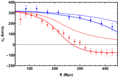
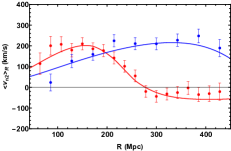
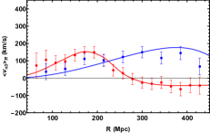
Figure 14: The bulk velocity $v_{\rm b}=\langle v_{n1}\rangle_{R}$ (left), together with the mean value of the quadrupole (centre) and octupole (right) of the peculiar radial velocity field, estimated using eq. (50), are shown as a function of the radius $R$ of the averaging volume. Dots represent the value inferred from discrete sampling (15,000 objects), while the continuous lines represent the underlying continuous field value. The red/ blue colors indicate results from the $M1/M2$ simulations. The dashed curves in the left panel present the estimates of the bulk velocity reconstructed by averaging the $3D$ peculiar velocity field, $v_{\rm b}=\langle v\rangle_{R}$.

X Conclusions

In local regions of the Universe, matter density fluctuations are so large in terms of amplitude and spatial scales that the application of the Cosmological Principle and the cosmological laws derived from it is problematic. Perturbation theory is certainly a powerful method for modelling and interpreting deviations from ideal uniform conditions. However, this approach has the drawback of requiring the assumption of a background cosmological metric. Can inhomogeneities and anisotropies be quantified in a model-independent way? Are there ways to let the data speak for themselves without assuming a priori FLRW scenarios or splitting the observed signals into a background and a perturbed component? Can we access the physical content of the measurements in a fully covariant way (see Maartens et al. (2023)) and yet determine the motion of the observer with respect to the surrounding matter frame?

We address these challenges using the expansion rate fluctuation field $\eta$, a statistically unbiased, Gaussian, scalar field that is sensitive to deviations from isotropy of the redshift-distance relationship. In Kalbouneh et al. (2023) it is shown how to extract the multipole moments of this observable. By analyzing its structure, it is found that unexpected symmetries characterize the local spacetime. Here we show that, in addition to its simple statistical properties, this observable also has a distinctive theoretical appeal. It allows us to constrain relevant cosmological quantities in a fully model-independent way.

Our main conclusions are as follows.

1. We provide a formula to predict, up to $\mathcal{O}(z^{3})$, the redshift scaling of the expansion rate fluctuation field. Its amplitude depends on the lower-order covariant cosmographic parameters that characterize in a model-independent way the structure of a generic spacetime in the surroundings of the event of observation, namely $\mathbb{H}$ (Hubble), $\mathbb{Q}$ (deceleration), $\mathbb{J}$ (jerk) and $\mathbb{R}$ (curvature).

2. The formalism is developed in such a way that it is straightforward to adapt it to observations carried out in a reference frame which is comoving with matter or in an arbitrary frame boosted with respect to it. It is crucial to carefully characterize the frame in which data is observationally measured and the frame in which quantities are theoretically characterized. Indeed the covariant cosmographic parameters at the event of observation have, in general, different amplitudes depending on the observer’s state of motion at that event Maartens et al. (2023). We show that it is practical to estimate the $\eta$ signal in the CMB frame, the frame of an observer who measures no CMB dipole, whatever the physical origin of that dipole is. At the same time, it is theoretically more convenient and natural to interpret the physical content of the signal in the matter frame, that of an observer at rest with respect to the surrounding matter fluid.

3. We have made explicit the dependence of the spherical harmonic components of $\eta$ on the multipoles of the covariant cosmographic parameters for a matter-comoving observer and in an axially symmetric configuration. According to the finding of Kalbouneh et al. (2023), this axial symmetry fairly well describes available data in the local Universe. A schematic summary of these relations is presented in FIG. 15. The dipole of $\eta$, when reconstructed in the CMB frame, provides unique information about the velocity of the observer relative to the matter frame. However, in order to infer the amplitude of this relative motion, it is necessary to disentangle it from the intrinsic distortions contributed by inhomogeneities in the metric. The latter effects are all the more important the deeper the volume analyzed. The next multipole of $\eta$, the quadrupole, is mainly sensitive to the ratio between the quadrupole and the monopole of the covariant Hubble parameter ($\mathbb{H}_{2}/\mathbb{H}_{0}$), although it also contains information about the quadrupole of the deceleration parameter.

4. By exploiting a simple analytical toy model of metric perturbations, we highlight the virtues and also the limitations of a power series expansion of $\eta$ as a function of redshift. Surprisingly, we find that the cosmographic expansion works well even in the local Universe, where large deviations in the distance-redshift relation, induced by density fluctuations, are expected. In particular, we show how to use the redshift evolution of $\eta$ multipoles to identify the redshift intervals where the cosmographic expansion breaks down and those where a meaningful theoretical inference can be made.

5. By randomly sampling the continuous toy model, we simulate all-sky catalogs of distances (typically containing 15,000 entries in the redshift interval $0<z<0.1$ and with Gaussian error in the distance modulus $\sigma_{\mu}=0.15$). We use them to assess the precision and accuracy with which future datasets, such as that under collection by the ZTF survey, will constrain the velocity of the observer (relative to the surrounding matter frame) and the multipoles of the covariant cosmographic parameters.

6. We also explore the cosmological potential of a more conventional analysis, in which the $\eta$ signal is interpreted in the context of the standard cosmological model. We show that in this case, the multipoles of $\eta$ provide insights into the amplitude of the multipoles of the radial peculiar velocity field of galaxies. Notably, the dipole of $\eta$ extracted in a given volume $V$ is proportional to the amplitude of the bulk motion on that characteristic scale.

Looking ahead to the future, we aim to build on current work and extend it in complementary directions. From an empirical point of view, we plan to estimate the expansion rate fluctuations from updated datasets which have recently become available, i.e., the Cosmicflows4 catalog Tully et al. (2023) and the Pantheon+ sample Brout et al. (2022). In addition, we aim to make more accurate predictions of the ZTF survey’s potential to constrain covariant cosmographic parameters, taking into account possible covariances in data uncertainties and more accurate maps of the celestial distribution of sources. From the theoretical side, we aim to exploit these insights into the structure of the local Universe in order to construct a spacetime metric that captures the essential features of the anisotropic $\eta$ signal. Finally, from the methodological side, we need to develop reconstruction techniques that allow us to estimate the expansion rate fluctuation field even from data with partial (and anisotropic) sky coverage. The purpose is to extend the multipolar analysis of the redshift-distance relation to the high redshift Universe.

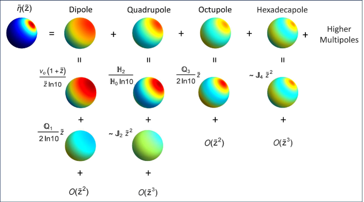
Figure 15: Graphic summary illustrating the decomposition of the expansion rate fluctuation field inferred in the CMB frame ($\tilde{\eta}$) in a given shell $S$ at redshift $\tilde{z}$, in terms of its axially-symmetric multipoles (horizontal direction). Each multipole is further related (vertical direction) to the dominant physical quantities contributing to its amplitude: these are the multipoles of the (lower-order) covariant cosmographic parameters and the relative velocity $v_{o}$ of the observer relative to the matter frame.

Appendix A Light Geodesics in Einstein de Sitter Spacetime

Consider the FLRW metric

$$\mathrm{d}s^{2}=-\mathrm{d}t^{2}+a^{2}(t)\left[\mathrm{d}r^{2}+r^{2}(\mathrm{d}\psi^{2}+\sin^{2}\psi\,\mathrm{d}\phi^{2})\right],$$ (51)

with an off-centre observer at a distance $r_{o}$ from the center of the coordinates (at $r=0$). We choose the $Z$-axis along this direction. The past pointing 4-wavevector of light is

$$k^{\mu}=\frac{\mathrm{d}x^{\mu}}{\mathrm{d}\lambda}\,,$$ (52)

where $\lambda$ is an affine parameter. We determine the geodesic path by solving the geodesic equations

$$\frac{\mathrm{d}^{2}x^{\mu}}{\mathrm{d}\lambda^{2}}+\Gamma^{\mu}_{\;\;\nu\alpha}\frac{\mathrm{d}x^{\nu}}{\mathrm{d}\lambda}\frac{\mathrm{d}x^{\alpha}}{\mathrm{d}\lambda}=0\,.$$ (53)

For the off-center observer, $k^{3}=0$ by symmetry. We choose the affine parameter as the physical distance measured by an observer at rest in the smooth background, with 4-velocity $\tilde{u}^{\mu}=\delta^{\mu}_{0}$, so that $\lambda=0$ at the observer position and $(k^{\mu}\tilde{u}_{\mu})_{o}=1$. The initial conditions are

$$t(0)=t_{0}\,,\;\;\;\;\;\;r(0)=r_{o}\,,\;\;\;\;\;\;\psi(0)=0\,,\quad\frac{\mathrm{d}t}{\mathrm{d}\lambda}\bigg{|}_{0}=-1\,,\;\;\;\;\;\;\frac{\mathrm{d}r}{\mathrm{d}\lambda}\bigg{|}_{0}=-\cos\theta\,,\;\;\;\;\;\;\frac{\mathrm{d}\psi}{\mathrm{d}\lambda}\bigg{|}_{0}=\frac{1}{r_{o}}\sin\theta\,,$$ (54)

where $t_{0}$ is the time of observation (today), and $\theta$ is the angle between the $Z$-axis and the direction the light ray measured by the observer $\tilde{u}^{\mu}$. The photon trajectory is thus

$$t(\lambda) =t_{0}\left(1-\frac{5}{3}\frac{\lambda}{t_{0}}\right)^{3/5}$$ (55)

$$r(\lambda) =r_{o}\left\{1+6\cos{\theta}\frac{t_{0}}{r_{o}}\left[\left(1-\frac{5}{3}\frac{\lambda}{t_{0}}\right)^{1/5}-1\right]+9\frac{t_{0}^{2}}{r_{o}^{2}}\left[\left(1-\frac{5}{3}\frac{\lambda}{t_{0}}\right)^{1/5}-1\right]^{2}\right\}^{1/2}\,,$$ (56)

$$\psi(\lambda) =\tan^{-1}(\cot\theta)-\tan^{-1}\left\{\cot\theta+3\frac{t_{0}}{r_{o}}\left[\left(1-\frac{5\lambda}{3t_{0}}\right)^{1/5}-1\right]\csc\theta\right\}.$$ (57)

By using eq. (38) and eq. (40), we can then infer the value of the redshift and luminosity distance.

Appendix B Multipoles of the Toy Model Cosmographic Parameters

We compute, at leading order of approximation, the explicit form of the multipoles of the covariant cosmographic parameters for the toy model presented in Sec. V. We do this by evaluating (5), (6), (7) and (8), using the toy-model prescriptions (34), (31) and (29). In order to simplify the equation, we define the dimensionless quantities $\xi_{o}\equiv R_{s}/r_{o}$ and $\xi_{H}\equiv R_{s}/R_{H}=R_{s}H_{0}$. All the multipoles $\ell\geq 5$ vanish at linear order in the perturbation parameter $\delta_{c}$. The only nonzero multipoles are

$$\mathbb{H}_{0} =H_{0}\left[1-\frac{1}{3}\delta_{c}\>\xi_{o}\left(\frac{\xi_{o}^{2}}{(1+\xi_{o}^{2})^{3/2}}-\frac{9}{2}\xi_{H}^{2}\operatorname{csch}^{-1}(\xi_{o})\right)\right],$$ (58)

$$\mathbb{H}_{2} =\frac{2\delta_{c}H_{0}\xi_{o}^{3}}{3(1+\xi_{o})^{3/2}}\left[-4-3\xi_{o}^{2}+3(1+\xi_{o}^{2})^{3/2}\operatorname{csch}^{-1}(\xi_{o})\right],$$ (59)

$$\mathbb{Q}_{0} =q_{0}+\frac{5\delta_{c}\xi_{o}^{3}}{6\left(1+\xi_{o}^{2}\right)^{3/2}},$$ (60)

$$\mathbb{Q}_{1} =-\frac{9\delta_{c}\xi_{o}^{4}}{5\xi_{H}(1+\xi_{o}^{2})^{5/2}},$$ (61)

$$\mathbb{Q}_{2} =-\frac{5}{2}\frac{\mathbb{H}_{2}}{H_{0}}\,,$$ (62)

$$\mathbb{Q}_{3} =\frac{2\delta_{c}\xi_{o}^{4}}{5\xi_{H}(1+\xi_{o}^{2})^{5/2}}\left[15(1+\xi_{o}^{2})^{5/2}\operatorname{csch}^{-1}(\xi_{o})-23-35\xi_{o}^{2}-15\xi_{o}^{4}\right],$$ (63)

$$\mathbb{R}_{0} =1-2\mathbb{Q}_{0}\,,$$ (64)

$$\mathbb{R}_{1} =\mathbb{Q}_{1}\,,$$ (65)

$$\mathbb{R}_{2} =-\frac{\mathbb{Q}_{2}}{5},$$ (66)

$$\mathbb{R}_{3} =\mathbb{Q}_{3}\,,$$ (67)

$$\mathbb{J}_{0} =j_{0}-\frac{\delta_{c}\xi_{o}^{3}}{15\xi_{H}^{2}(1+\xi_{o}^{2})^{7/2}}\left[9\xi_{o}^{2}(2-3\xi_{o}^{2})-25\xi_{H}^{2}(1+\xi_{o}^{2})^{2}\right],$$ (68)

$$\mathbb{J}_{1} =-\mathbb{Q}_{1}\,,$$ (69)

$$\mathbb{J}_{2} =-\frac{10\delta_{c}\xi_{o}^{3}}{21\xi_{H}^{2}(1+\xi_{o}^{2})^{7/2}}\left[18\xi_{o}^{2}-7(1+\xi_{o}^{2})^{2}(4+3\xi_{o}^{2})\xi_{H}^{2}+21\xi_{H}^{2}(1+\xi_{o}^{2})^{7/2}\operatorname{csch}^{-1}(\xi_{o})\right],$$ (70)

$$\mathbb{J}_{3} =-\mathbb{Q}_{3}\,,$$ (71)

$$\mathbb{J}_{4} =\frac{8\delta_{c}\xi_{o}^{5}}{35\xi_{H}^{2}(1+\xi_{o}^{2})^{7/2}}\left[105(1+\xi_{o}^{2})^{7/2}\operatorname{csch}^{-1}(\xi_{o})-7\xi_{o}^{2}(58+50\xi_{o}^{2}+15\xi_{o}^{4})-176\right].$$ (72)

Note that, in addition to the monopole of the deceleration parameter $\mathbb{Q}$, which mainly comes from the background, the dominant multipoles of $\mathbb{Q}$ are the dipole and the octupole – since they are proportional to $1/\xi_{H}$. They compensate for the smallness of $z$ in the Taylor expansion of eqs. (22) and (24) when the size of the perturbations is comparable with the redshift of volume under study. For the jerk parameter $\mathbb{J}$, the dominant multipoles are the even multipoles (monopole, quadrupole, hexadecapole), since they are proportional to $1/\xi_{H}^{2}$, which compensates the smallness of $z^{2}$ in eqs. (21) and (23).

Appendix C Legendre Coefficients Estimation

We show here how we calculate the Legendre coefficients of an axisymmetric field $\eta$. For each spherical shell $S$ at redshift $z$ and with thickness $\delta z$, we calculate the angle $\theta$ between the angular position of each galaxy $j$ contained in the shell $(l_{j},b_{j})$, and the axis of symmetry $(l_{a},b_{a})$:

$$\cos(\theta_{j})=\sin(b_{j})\sin(b_{a})+\cos(b_{j})\cos(b_{a})\cos(l_{j}-l_{a})\,.$$ (73)

We then split the shell into $N_{\rm bins}$ equal bins in $\cos\theta$ and calculate $\nu\equiv\log(z/d_{L})=\log(z)+5-\frac{\mu}{5}$ for each galaxy in the bin, and calculate the weighted average of $\nu$:

$$\bar{\nu}(\cos\theta_{i})={\sum_{j=1}^{(N_{\rm gal})_{i}}\frac{\nu(j)}{\delta_{j}^{2}}}\,\left[{\sum_{j=1}^{(N_{\rm gal})_{i}}\frac{1}{\delta_{j}^{2}}}\right]^{-1}\,.$$ (74)

Here $(N_{\rm gal})_{i}$ is the number of galaxies in the bin $(\Delta\cos\theta)_{i}$, where $i$ runs from 1 to $N_{\rm bins}$ ($\theta_{i}$ is the angle calculated at the middle of the bin), and $\delta_{j}$ is the error of $\nu(j)$, which is induced by the uncertainty of the distance modulus ($\sigma_{\mu}$) of each galaxy ($\delta_{j}=\sigma_{\mu_{j}}/5$). The zeroth order estimator of the Legendre coefficients is

$$\nu_{\ell}^{(0)}=\frac{2\ell+1}{N_{\rm bins}}\sum_{i=1}^{N_{\rm bins}}\bar{\nu}(\cos\theta_{i})\,P_{\ell}(\cos\theta_{i})\,.$$ (75)

The number $N_{\rm bins}$ must be larger than the number of multipoles one wants to compute (we stop at $\ell=4$), but small enough such that all the bins have galaxies inside, so we set it to be $15$. We compute the higher-order refinements iteratively, according to a formula similar to that used by HEALPix Górski et al. (2005), in order to estimate the spherical harmonic coefficients of a generic, non-axisymmetric field:

$$\nu_{\ell}^{(k+1)}=\nu_{\ell}^{(k)}+\frac{2\ell+1}{N_{\rm bins}}\sum^{N_{\rm bins}}_{i=1}\Big{[}\bar{\nu}(\cos\theta_{i})-\bar{\nu}^{(k)}(\cos\theta_{i})\Big{]}\,P_{\ell}(\cos\theta_{i})\,,$$ (76)

where

$$\bar{\nu}^{(k)}(\cos\theta_{i})=\sum^{\ell_{\rm max}}_{\ell=0}\nu_{\ell}^{(k)}P_{\ell}(\cos\theta_{i})\,.$$ (77)

We choose $\ell_{\rm max}=4$, which is the maximum dominant multipole of the Jerk, the highest order covariant cosmographic parameter considered in our analysis. Note that for the case under study the iteration becomes stable after about 5 loops, so we stop the process for $k_{max}=10$. Concerning the variance of $\eta_{\ell}$, we proceed as follows. We calculate the variance of the zeroth order estimator $\nu_{\ell}^{(0)}$, which is

$$V[\nu_{\ell}^{(0)}]=\left(\frac{2\ell+1}{N_{\rm bins}}\right)^{2}\sum_{i=1}^{N_{\rm bins}}\big{[}\sigma_{\nu(i)}P_{\ell}(\cos\theta_{i})\big{]}^{2}\,,$$ (78)

where $\sigma_{\nu(i)}^{2}$ is the variance of $\nu(\cos\theta_{i})$:

$$\sigma_{\nu(i)}^{2}=\left[{\sum_{j=1}^{(N_{\rm gal})_{i}}\frac{1}{\delta_{j}^{2}}}\right]^{-1}\,$$ (79)

Since $\mathcal{M}=\nu_{0}$ and $\eta_{\ell}=\nu_{\ell}^{(k_{max})}$, we set

$$\sigma_{\mathcal{M}}^{2}=V[\nu_{0}^{(0)}]\,,$$ (80)

$$\sigma_{\eta_{\ell}}^{2}=V[\nu_{\ell}^{(0)}]\,,$$ (81)

which provide excellent approximations as we tested with simulations. This process can be used equivalently for reconstructing $\eta$ in the matter frame or in the CMB frame. If the distribution of the points is isotropic over the sky and the uncertainty in the distance modulus is the same for all objects, then we can approximate the variance of $\nu_{\ell}$ by

$$V[\nu_{\ell}]=\frac{2\ell+1}{N_{\rm gal}^{\text{inside the shell}}}\,\frac{\sigma_{\mu}^{2}}{25}\,$$ (82)

which does not depend on the choice of the number of bins $N_{\rm bins}$.

Appendix D Correlation between Multipoles of the Expansion Rate Fluctuation

The $\chi^{2}$ minimization (see eq. (47)) was performed by ignoring the correlation between the multipoles of $\eta$, i.e., by assuming that the covariance matrix and its inverse (the precision matrix) are diagonal. Here, for completeness, we justify this choice. We present the correlation matrix for some specific redshift shells of the model $M2$. We generate 50,000 samples with distance moduli randomly simulated around the measured value, and calculate the correlation matrix as

$$\text{Corr}_{\ell\ell^{\prime}}=\frac{\big{\langle}(\boldsymbol{\nu}_{\ell}-\langle\boldsymbol{\nu}_{\ell}\rangle)(\boldsymbol{\nu}_{\ell^{\prime}}-\langle\boldsymbol{\nu}_{\ell^{\prime}}\rangle)\big{\rangle}}{\sigma_{\boldsymbol{\nu}_{\ell}}\sigma_{\boldsymbol{\nu}_{\ell^{\prime}}}}\,.$$ (83)

Here angled brackets denote the average and $\sigma_{\boldsymbol{\nu}_{\ell}}$ is the standard deviation of the multipole $\ell$ of $\nu$, where $\nu$ is defined in Appendix C ($\mathcal{M}=\nu_{0}$, $\eta_{\ell}=\nu_{\ell}$ for $\ell>0$). The elements of the correlation matrix at three different depths are

$$\text{\bf Corr}\,(\tilde{z}=0.015)=\left(\begin{array}[]{cccc}1&0.03&-0.06&-0.04\\ 0.03&1&-0.01&0.06\\ -0.06&-0.01&1&0.04\\ -0.04&0.06&0.04&1\\ \end{array}\right),$$ (84)

$$\text{\bf Corr}\,(\tilde{z}=0.055)=\left(\begin{array}[]{cccc}1&0.024&0.001&0.002\\ 0.024&1&0.02&-0.001\\ 0.001&0.02&1&0.05\\ 0.002&-0.001&0.05&1\\ \end{array}\right),$$ (85)

$$\text{\bf Corr}\,(\tilde{z}=0.095)=\left(\begin{array}[]{cccc}1&-0.041&-0.006&-0.027\\ -0.041&1&-0.062&-0.007\\ -0.006&-0.062&1&-0.001\\ -0.027&-0.007&-0.001&1\\ \end{array}\right).$$ (86)

The off-diagonal elements are indeed small and can be safely neglected.

References

- Di Valentino et al. (2021) E. Di Valentino, O. Mena, S. Pan, L. Visinelli, W. Yang, A. Melchiorri, D. F. Mota, A. G. Riess, and J. Silk, Class. Quant. Grav. 38, 153001 (2021), eprint 2103.01183.
- Abdalla et al. (2022) E. Abdalla et al., JHEAp 34, 49 (2022), eprint 2203.06142.
- Perivolaropoulos and Skara (2022) L. Perivolaropoulos and F. Skara, New Astron. Rev. 95, 101659 (2022), eprint 2105.05208.
- Schöneberg et al. (2022) N. Schöneberg, G. Franco Abellán, A. Pérez Sánchez, S. J. Witte, V. Poulin, and J. Lesgourgues, Phys. Rept. 984, 1 (2022), eprint 2107.10291.
- Schwarz and Weinhorst (2007) D. J. Schwarz and B. Weinhorst, Astron. Astrophys. 474, 717 (2007), eprint 0706.0165.
- Kashlinsky et al. (2009) A. Kashlinsky, F. Atrio-Barandela, D. Kocevski, and H. Ebeling, Astrophys. J. Lett. 686, L49 (2009), eprint 0809.3734.
- Antoniou and Perivolaropoulos (2010) I. Antoniou and L. Perivolaropoulos, JCAP 12, 012 (2010), eprint 1007.4347.
- Cai and Tuo (2012) R.-G. Cai and Z.-L. Tuo, JCAP 02, 004 (2012), eprint 1109.0941.
- Kalus et al. (2013) B. Kalus, D. J. Schwarz, M. Seikel, and A. Wiegand, Astron. Astrophys. 553, A56 (2013), eprint 1212.3691.
- Wang and Wang (2014) J. S. Wang and F. Y. Wang, Mon. Not. Roy. Astron. Soc. 443, 1680 (2014), eprint 1406.6448.
- Yoon et al. (2014) M. Yoon, D. Huterer, C. Gibelyou, A. Kovács, and I. Szapudi, Mon. Not. Roy. Astron. Soc. 445, L60 (2014), eprint 1406.1187.
- Tiwari and Nusser (2016) P. Tiwari and A. Nusser, JCAP 03, 062 (2016), eprint 1509.02532.
- Javanmardi et al. (2015) B. Javanmardi, C. Porciani, P. Kroupa, and J. Pflamm-Altenburg, Astrophys. J. 810, 47 (2015), eprint 1507.07560.
- Bengaly (2016) C. A. P. Bengaly, Jr., JCAP 04, 036 (2016), eprint 1510.05545.
- Colin et al. (2017) J. Colin, R. Mohayaee, M. Rameez, and S. Sarkar, Mon. Not. Roy. Astron. Soc. 471, 1045 (2017), eprint 1703.09376.
- Rameez et al. (2018) M. Rameez, R. Mohayaee, S. Sarkar, and J. Colin, Mon. Not. Roy. Astron. Soc. 477, 1772 (2018), eprint 1712.03444.
- Migkas et al. (2020) K. Migkas, G. Schellenberger, T. H. Reiprich, F. Pacaud, M. E. Ramos-Ceja, and L. Lovisari, Astron. Astrophys. 636, A15 (2020), eprint 2004.03305.
- Migkas et al. (2021) K. Migkas, F. Pacaud, G. Schellenberger, J. Erler, N. T. Nguyen-Dang, T. H. Reiprich, M. E. Ramos-Ceja, and L. Lovisari, Astron. Astrophys. 649, A151 (2021), eprint 2103.13904.
- Secrest et al. (2021) N. J. Secrest, S. von Hausegger, M. Rameez, R. Mohayaee, S. Sarkar, and J. Colin, Astrophys. J. Lett. 908, L51 (2021), eprint 2009.14826.
- Siewert et al. (2021) T. M. Siewert, M. Schmidt-Rubart, and D. J. Schwarz, Astron. Astrophys. 653, A9 (2021), eprint 2010.08366.
- Luongo et al. (2022) O. Luongo, M. Muccino, E. O. Colgáin, M. M. Sheikh-Jabbari, and L. Yin, Phys. Rev. D 105, 103510 (2022), eprint 2108.13228.
- Krishnan et al. (2022) C. Krishnan, R. Mohayaee, E. O. Colgáin, M. M. Sheikh-Jabbari, and L. Yin, Phys. Rev. D 105, 063514 (2022), eprint 2106.02532.
- Sorrenti et al. (2023) F. Sorrenti, R. Durrer, and M. Kunz, JCAP 11, 054 (2023), eprint 2212.10328.
- Aluri et al. (2023) P. K. Aluri et al., Class. Quant. Grav. 40, 094001 (2023), eprint 2207.05765.
- Cowell et al. (2023) J. A. Cowell, S. Dhawan, and H. J. Macpherson, Monthly Notices of the Royal Astronomical Society 526, 1482–1494 (2023).
- Hu et al. (2023) J. P. Hu, Y. Y. Wang, J. Hu, and F. Y. Wang (2023), eprint 2310.11727.
- Dainotti et al. (2021) M. G. Dainotti, B. De Simone, T. Schiavone, G. Montani, E. Rinaldi, and G. Lambiase, Astrophys. J. 912, 150 (2021), eprint 2103.02117.
- Marinoni et al. (2012) C. Marinoni, J. Bel, and A. Buzzi, JCAP 10, 036 (2012), eprint 1205.3309.
- Hoffman et al. (2017) Y. Hoffman, D. Pomarede, R. Brent Tully, and H. Courtois (2017), eprint 1702.02483.
- Strauss and Willick (1995) M. A. Strauss and J. A. Willick, Phys. Rept. 261, 271 (1995), eprint astro-ph/9502079.
- Maartens et al. (2023) R. Maartens, J. Santiago, C. Clarkson, B. Kalbouneh, and C. Marinoni (2023), eprint 2312.09875.
- Colin et al. (2019) J. Colin, R. Mohayaee, M. Rameez, and S. Sarkar (2019), eprint 1912.04257.
- Rubin and Heitlauf (2020) D. Rubin and J. Heitlauf, Astrophys. J. 894, 68 (2020), eprint 1912.02191.
- Dhawan et al. (2022a) S. Dhawan, A. Borderies, H. J. Macpherson, and A. Heinesen, Monthly Notices of the Royal Astronomical Society 519, 4841–4855 (2022a).
- Kalbouneh et al. (2023) B. Kalbouneh, C. Marinoni, and J. Bel, Phys. Rev. D 107, 023507 (2023), eprint 2210.11333.
- Amenouche (2022) M. Amenouche, Phd thesis, Université Clermont Auvergne (2022), URL theses.hal.science/tel-04165406.
- Kristian and Sachs (1966) J. Kristian and R. K. Sachs, The Astrophysical Journal 143, 379 (1966).
- Ellis (2009) G. F. Ellis, General Relativity and Gravitation 41, 581–660 (2009).
- MacCallum and Ellis (1970) M. A. MacCallum and G. F. Ellis, Communications in Mathematical Physics 19, 31–64 (1970).
- Clarkson (2000) C. A. Clarkson, Phd thesis, University of Glasgow (2000), URL arxiv.org/abs/astro-ph/0008089.
- Clarkson and Maartens (2010) C. Clarkson and R. Maartens, Classical and Quantum Gravity 27, 124008 (2010).
- Heinesen (2021) A. Heinesen, Journal of Cosmology and Astroparticle Physics 05, 008 (2021).
- Visser (2004) M. Visser, Classical and Quantum Gravity 21, 2603–2615 (2004).
- Hui and Greene (2006) L. Hui and P. B. Greene, Physical Review D 73 (2006).
- Bonvin et al. (2006) C. Bonvin, R. Durrer, and M. A. Gasparini, Physical Review D 73 (2006).
- Tully et al. (2016) R. B. Tully, H. M. Courtois, and J. G. Sorce, The Astronomical Journal 152, 50 (2016).
- Scolnic et al. (2018) D. M. Scolnic, D. O. Jones, A. Rest, Y. C. Pan, R. Chornock, R. J. Foley, M. E. Huber, R. Kessler, G. Narayan, A. G. Riess, et al., Astrophys. J. 859, 101 (2018), eprint 1710.00845.
- Horstmann et al. (2022) N. Horstmann, Y. Pietschke, and D. J. Schwarz, Astron. Astrophys. 668, A34 (2022), eprint 2111.03055.
- Marinoni et al. (1998) C. Marinoni, P. Monaco, G. Giuricin, and B. Costantini, The Astrophysical Journal 505, 484–505 (1998).
- Peebles (1980) P. J. Peebles, The large-scale structure of the universe (Princeton University Press, 1980).
- Fleury (2015) P. Fleury, Ph.D. thesis, Paris U., VI, IAP (2015), eprint 1511.03702.
- Durrer (2021) R. Durrer, The cosmic microwave background (Cambridge University Press, 2021).
- Tully et al. (2019) R. B. Tully, D. Pomarède, R. Graziani, H. M. Courtois, Y. Hoffman, and E. J. Shaya, The Astrophysical Journal 880, 24 (2019).
- Dhawan et al. (2022b) S. Dhawan, A. Goobar, J. Johansson, I. S. Jang, M. Rigault, L. Harvey, K. Maguire, W. L. Freedman, B. F. Madore, M. Smith, et al., The Astrophysical Journal 934, 185 (2022b).
- Heinesen and Macpherson (2022) A. Heinesen and H. J. Macpherson, Journal of Cosmology and Astroparticle Physics 2022, 057 (2022).
- Nusser (2015) A. Nusser, Monthly Notices of the Royal Astronomical Society 455, 178–184 (2015).
- Tully et al. (2023) R. B. Tully et al., Astrophys. J. 944, 94 (2023), eprint 2209.11238.
- Brout et al. (2022) D. Brout et al., Astrophys. J. 938, 110 (2022), eprint 2202.04077.
- Górski et al. (2005) K. M. Górski, E. Hivon, A. J. Banday, B. D. Wandelt, F. K. Hansen, M. Reinecke, and M. Bartelman, Astrophys. J. 622, 759 (2005), eprint astro-ph/0409513.