Efficient Paths for Local Counterdiabatic Driving
Abstract
Local counterdiabatic driving (CD) provides a feasible approach for realizing approximate reversible/adiabatic processes like quantum state preparation using only local controls and without demanding excessively long protocol times. However, in many instances getting high accuracy of such CD protocols requires engineering very complicated new controls or pulse sequences. In this work, we describe a systematic method for altering the adiabatic path by adding extra local controls along which performance of local CD protocols is enhanced. We then show that this method provides dramatic improvement in the preparation of non-trivial GHZ ground states of several different spin systems with both short-range and long-range interactions.
I Introduction
With the rapid development of quantum technologies such as quantum computing, as well as the demands of modern experiments with e.g. cold atoms van Frank et al. (2016), trapped ions Senko et al. (2015) and nitrogen-vacancy centers Rembold et al. (2020), precise control over quantum states is essential. Adiabatic processes present a powerful tool for manipulating these states, where any changes to the system are made sufficiently slowly so that the quantum state remains in an instantaneous eigenstate at all times, allowing for precise control.
However, even in the finite-size systems accessible to near-term quantum computers and modern experimental setups, the timescales required for adiabaticity are often longer than the system remains coherent and thus forbid its application. This has motivated the development of so-called “Shortcuts to adiabaticity” Guéry-Odelin et al. (2019) in which the adiabatic path may be approximately or exactly followed at faster timescales, at the expense of demanding additional control over the system.
One such technique is known as counterdiabatic (CD) driving or equivalently transitionless driving Demirplak and Rice (2003, 2005); Berry (2009); Hartmann and Lechner (2019); Wurtz and Love (2022); Chandarana et al. (2022); Schindler and Bukov (2023), where an additional counterdiabatic term is added to the Hamiltonian of the system, which exactly suppresses any transitions between states arising from a fast change of parameters. With this modified Hamiltonian the initial quantum state, which evolves according to the Schrödinger equation, will now following the instantaneous eigenstates by construction.
While this procedure is always exact, the CD term in general requires knowledge of the full spectrum of the system and is thus not accessible for generic many-body systems. This has lead to the development of local CD driving Sels and Polkovnikov (2017); Claeys et al. (2019) in which the CD term is restricted to only local operators at the price of failing to completely suppress all transitions. Nonetheless, it yields protocols which can significantly increase the fidelity of the prepared quantum state while remaining feasible to actually implement.
Recently, it has been shown that by combining approaches from quantum optimal control Stefanatos and Paspalakis (2021), whereby additional control terms are added to the system, and then performing local CD driving, quantum states may be prepared with higher fidelity than local CD driving alone Čepaitė et al. (2023). However, it is not immediately clear what these additional control terms should be.
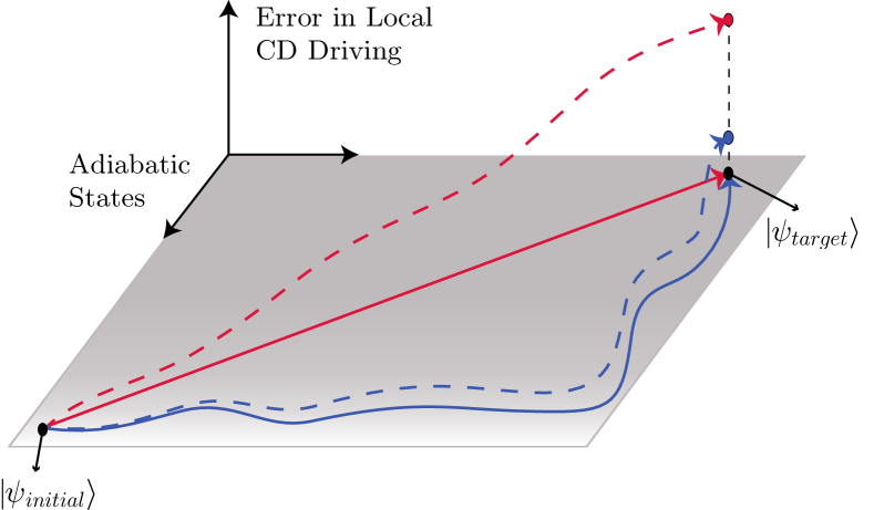
The main purpose of this work is to propose a systematic method for adding such extra local controls to the Hamiltonian along which local CD protocols are most efficient. Schematically the idea is sketched conceptually in Figure 1. The horizontal plane represents the space of adiabatically connected ground states. By introducing extra controls we can modify the adiabatic path connecting the initial and final states (solid lines). The vertical line schematically represents an error (e.g. deviation of the fidelity from unity) resulting from the local CD driving (dashed lines). The optimal (blue) path results in a lower error. Note that while we focus on quantum state preparation this formalism can be applied to realize fast and reversible energy transfer to facilitate various thermodynamic processes Villazon et al. (2019); Gjonbalaj et al. (2022).
This paper is organized as follows: in Section II we review how quantum states may be prepared adiabatically, when this fails, and how counterdiabatic driving may be employed to alleviate this. In Section III we discuss how we may employ local (approximate) counterdiabatic driving most efficiently by augmenting the underlying Hamiltonian with extra control terms. In Section IV we show how this may be applied beyond the standard short-range models, especially those connected to relevant experiments. Finally, we summarize in Section V and discuss potentially fruitful applications of these techniques beyond the contents of this paper.
II Counterdiabatic driving
One straightforward approach to preparing quantum states is to employ the adiabatic theorem. For a system whose energy levels have a finite gap, this guarantees Sakurai and Napolitano (2017) that if the control parameter of the Hamiltonian is changed sufficiently slowly, the system will always remain in an instantaneous eigenstate.
Let us consider a time dependent Hamiltonian , where the time dependence is encoded in a control parameter which varies from 0 to 1. While this may in general represent a vector of several control parameters, we will restrict ourselves to just one for simplicity. The adiabatic theorem guarantees that if our system begins in the ground state of , and the parameter is changed sufficiently slowly, the system will conclude the protocol in the ground state of .
One straightforward application of this is so-called quantum annealing, where the Hamiltonian is designed such that the final ground state at is the target state, which is usually difficult to prepare, but the initial ground state at is easy to prepare. By preparing the system in the initial state and then changing slowly, the target state may be obtained with arbitrarily high fidelity. However, the condition that be small can become quite restrictive as we move beyond simple systems and the gaps between energy levels become smaller.
Formally, the adiabatic approximation is made by writing the Schrödinger equation in the basis of instantaneous eigenstates, and then neglecting emergent rate dependent off-diagonal terms coupling different eigenstates Berry (2009); Kolodrubetz et al. (2017). This suggests that perfect adiabaticity may be obtained by inserting into the Hamiltonian some compensating terms which will exactly cancel those ignored in the adiabatic approximation. If this is done, the adiabatic approximation becomes exact irrespective of .
Counterdiabatic driving was first discovered by Demirplak & Rice Demirplak and Rice (2003, 2005) in the context of population transfer between molecular states, and independently formulated by Berry Berry (2009) and termed “transitionless driving,” although the two are entirely equivalent. This involves defining the counterdiabatic Hamiltonian such that
| (1) |
where is known as the adiabatic gauge potential (AGP). This operator is responsible for transforming the instantaneous eigenstates under a change of the control parameter .
Formally, the AGP satisfies the following equation
| (2) |
Despite its apparent simplicity, this equation is in general very difficult to solve. It can be shown Sels and Polkovnikov (2017) however that solving Eq. (2) is equivalent to minimizing the following action:
| (3) |
We note in passing that one can use replace , where is an arbitrary stationary density matrix with respect to the Hamiltonian Sels and Polkovnikov (2017). We may interpret Eq. (2), which in this language reads , as a statement that a well-defined AGP admits the existence of a conserved operator commuting with .
Instead of dealing with the exact AGP, which is very nonlocal and even ill-defined in chaotic systems Pandey et al. (2020), it is convenient to find an approximate local AGP, which minimizes the action in Eq. (3) within a restricted subset of operators . A very convenient option is to choose this subset from the so-called Krylov space, which is obtained by a repeated action of Liouvillian on Claeys et al. (2019):
| (4) |
Here controls the order (and therefore the locality) of the expansion, and are the variational parameters found by minimizing the action (3). Formally this ansatz is exact in the limit but in practice we want to restrict it to small values of . The variational method can be further improved by using the Lanczos algorithm in the operator basis leading to an AGP expansion in an orthonormal set of Krylov operators (see Refs. Takahashi and del Campo, 2023; Bhattacharjee, 2023; Sels and Polkovnikov, 2023 for details). We give a detailed description of our Krylov space construction of the AGP in Appendix A.
III Improving CD driving with extra controls
The main goal of this section and of the whole paper is to find a systematic approach to improving performance of approximate CD driving via adding extra controls and apply them to prepare nontrivial GHZ entangled states. We focus on the infinite speed limit , where effectively we evolve only according to the AGP as defined in Eq. (1).
Before proceeding with nontrivial systems, we illustrate the idea of extra controls using an intuitive example of ground state preparation in a one-dimensional Ising model with transverse and longitudinal fields described by a standard quantum annealing scheme Hauke et al. (2020):
| (5) |
with periodic boundary conditions. We will start from the situation where there is a small but finite longitudinal field and finite . The first condition breaks the symmetry of the model such that the ferromagnetic ground state for is polarized in the positive -direction and the second condition implies that during the annealing protocol the system crosses a quantum phase transition at Sachdev (2011). At this point the gap closes and the AGP becomes an operator with an infinite range del Campo et al. (2012); Damski (2014); Kolodrubetz et al. (2017) such that local CD protocols become very inefficient.
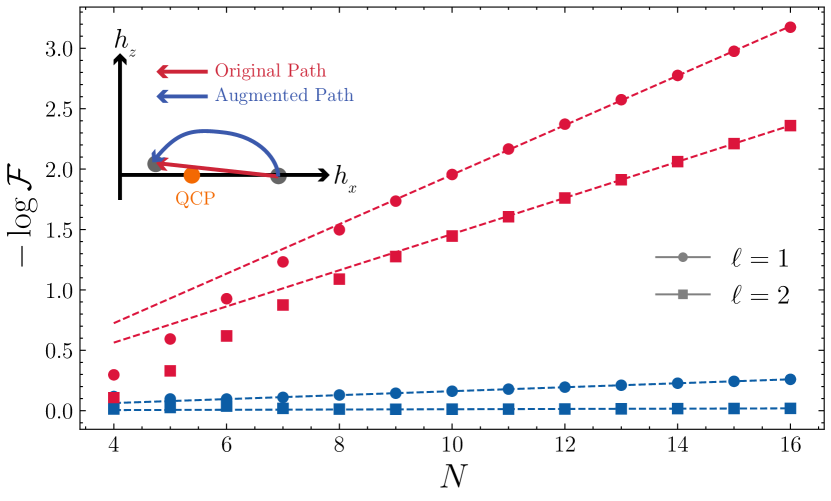
In this setup it should be clearly more advantageous to choose an alternate path, which while retaining the same start and end points, stays far away from the critical point. This is shown in the inset of Figure 2. Following the general idea of Ref. Čepaitė et al., 2023 the Hamiltonian corresponding to the modified path is given by
where is some parameter which we can optimize numerically. We then apply local CD driving to . With an appropriate choice of , this gives a very strong improvement in state preparation, as shown in Figure 2. In particular, we can see that even just the first two terms in the expansion in Equation (4) are sufficient to prepare the state with high fidelity nearly independent of system size despite the fact that is not very small and thus the ferromagnetic state is far from fully polarized.
III.1 Formulation of General Problem
The example above shows the utility of adding extra controls, which in that case can be intuitively found. Similar ideas without CD driving were experimentally implemented to prepare topological Hofstadter bands in ultracold atoms Aidelsburger et al. (2014). The question we aim to address is how can we find efficient extra controls for arbitrary Hamiltonians and . Formally we define an alternate path by evolving the system according to an augmented Hamiltonian
| (6) |
where ) is given by Eq. (5) and the are some smooth functions satisfying boundary conditions so that the initial and final eigenstates of the annealing Hamiltonian are unchanged. We refer to as an extra control Hamiltonian. In the previous example, it was just an additional global field, i.e. . We stress that in the infinite speed limit we follow only the AGP, so the annealing Hamiltonian plays a purely auxiliary role like e.g. in Ref. Ljubotina et al., 2022.
We then perform local CD driving for the augmented Hamiltonian , hence evolving according to . The goal is to choose both and to maximize the fidelity of the final state. Finding the optimal control functions is the subject of quantum optimal control Glaser et al. (2015) or similar methods Bukov et al. (2018), which is not the main focus of this work. We pick the by a very simple optimization, following earlier work Čepaitė et al. (2023), writing it as a single harmonic term
| (7) |
and choosing to maximize the fidelity of the final state. This is done by choosing the cost function
| (8) |
where is obtained by evolving the initial state by local corresponding to . We note that the fidelities can be even further improved by adding additional couplings corresponding to -th harmonic of Čepaitė et al. (2023). We limit ourselves only to the first one as we want to focus on the question of finding optimal .
III.2 Ansatz for Extra Controls
To proceed, let us consider a state preparation problem similar to the previous one, but with , i.e. without breaking the -symmetry. The ferromagnetic ground state of this model is now a GHZ state Greenberger et al. (2007). It is defined as an equal superposition of all spins up and all spins down. This adiabatic state preparation is encoded in the Hamiltonian
| (9) |
The previous choice of will not work, since it breaks the symmetry of the ground state of and allows one to prepare either the up or down polarized state, but not a superposition of both.
In order to identify the form of , we note that for any value of the AGP ansatz in Equation (4) is composed of odd commutators of the operators and like
In the AGP these commutators appear with different coefficients which depend on . Let us observe that the general composition of the operators entering the exact AGP (i.e. at all orders of the expansion in Eq. 4) will not change if we modify the Hamiltonian by adding arbitrary even order commutators to it, i.e. adding terms like
| (10) |
with the corresponding weights . By adding such terms we clearly expand the variational manifold allowing one to gradually increase locality of both and . Moreover such terms can be generated using Floquet pulse sequences containing only and as was done in Ref. Claeys et al., 2019 for realizing the AGP, and is routinely done in the NMR literature Farrar and Becker (1971). As we show below for the examples we analyze here this idea leads to the dramatic improvement of local CD protocols.
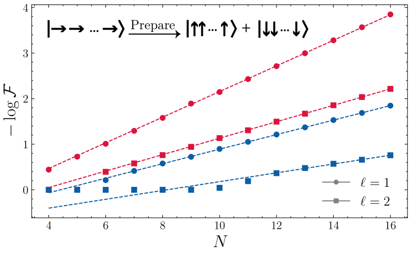
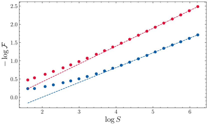
It is easy to check that for the Ising model the new terms (i.e. terms which are not originally present in ) which appear by computing the commutators in Eq. (10) are and , where we use a common short-hand notation: , . We can thus select and . In this way the augmented Hamiltonian (6) will cause the state to follow a genuinely new path. The resulting improvement of the final state fidelity is plotted in Figure 3. For a more detailed discussion of the optimization procedure see Appendix B.
We can see that the extra controls lead to a dramatic improvement of the protocol. In particular, for system sizes up to the second order AGP ansatz corresponding to in Eq. (4) leads to nearly unit fidelity. For larger system sizes the fidelity decays exponentially with with a reduced slope, and thus still offering exponential enhancement over the original CD protocol. We note that as we continue to increase the order of the AGP expansion the size of the system we can prepare with unit fidelity increases, as does the exponential enhancement in fidelity over the corresponding original CD protocol.
IV Preparing GHZ state in a Long range model.
We now move to preparation of the GHZ state in longer range Ising Hamiltonians, which are relevant to cold atom/trapped ion systems Koffel et al. (2012); Jaschke et al. (2017); Adelhardt et al. (2020). We define the annealing Hamiltonian for a long-range Ising model:
| (11) |
where . Note that we can interpolate between the short-range model studied earlier and a fully connected model by varying the exponent .
Let us first consider a long-range case with and then move to the fully connected model with . In both cases the naive path crosses a critical (gapless) point at some value of which depends on the parameter and additionally scales with for .
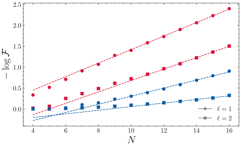
We then augment the original Hamiltonian by introducing extra controls
corresponding to the terms and in Eq. (10). Like in the previous example we then use a standard CD protocol and find the parameters and by optimizing the fidelity of the final state.
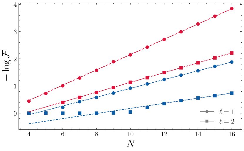
As shown in Figure 4 for the long-range Ising model, we again find a dramatic improvement of the GHZ state preparation along the optimally augmented path. We notice that this improvement is not tied in any way to the integrability (short range)/nonintegrability (long range) of the Ising model. This is not that surprising, as the short range AGP (small ) cannot distinguish integrable and nonintegrable systems Pandey et al. (2020) and extra controls generally break integrability anyway.
Finally, let us discuss the fully connected model corresponding to . With an appropriate rescaling of couplings, this model is equivalent to a single large spin with a nonlinear interaction. The corresponding annealing Hamiltonian is still given by Eq. (5) with
| (12) |
Here we rescale the first term so that the model has a well defined classical/thermodynamic limit as . We note in passing that this Hamiltonian is extensively employed for experimental preparation of spin squeezed states Kitagawa and Ueda (1993); Law et al. (2001); Rojo (2003); Sorensen and Molmer (2001). Such spin-squeezed states allow for better scaling of measurement precision in Ramsey interferometry, surpassing the Standard Quantum Limit Wineland et al. (1992); Bollinger et al. (1996). We show the results for this in Figure 5. Interestingly one of the emergent extra control Hamiltonians in Eq. 10 is , which is used in the two-axis twisting Hamiltonian for the preparation of even better spin-squeezed states.
As in both the short- and long-range spin models, we observe that we can prepare states with much better fidelity using these more efficient paths, though the improvement is less dramatic. The performance can be likely enhanced further by considering finite energy norms for the variational optimization of the action, as was done in a different classical model Gjonbalaj et al. (2022).
V Conclusions & Outlook
Counterdiabatic driving can prepare quantum states adiabatically on timescales that are much shorter than typical decoherence times. By restricting the locality of the CD driving, we can obtain experimentally-accessible protocols for approximately preparing the ground states of interesting many-body systems.
We have proposed a systematic method for finding extra control terms for quantum annealing protocols with which to augment a Hamiltonian, so that local CD driving prepares a target ground state with exponentially better fidelity. Phrased another way, our method specifies how to find the paths through the space of possible Hamiltonian couplings along which approximate CD driving will be most efficient. We find these paths by restricting the additional terms to those which preserve the commutator structure of the original CD driving term. These terms can be effectively engineered via Floquet protocols using only the original controls. We have tested this method on 1D spin chains with short- and long-range interactions and showed that it allows for strong improvement of preparation of GHZ states.
While this work has been principally concerned with proposing this technique and testing it with simple models, there are many others to which this recipe for more efficient paths might be applied. Going beyond one-dimensional systems, exploring models with frustration, or mappings to e.g. satisfiability problems on arbitrary graphs are all areas where this recipe may yield improvement.
Acknowledgments
This work was supported by NSF Grant DMR-2103658 and the AFOSR Grant FA9550-21-1-0342. The authors thank Aashish Clerk, Andrew Daley, Callum Duncan, Michael Flynn and Tatsuhiko Ikeda for helpful discussions. The authors acknowledge that the computational work reported in this paper was performed on the Shared Computing Cluster administered by Boston University’s Research Computing Services. The numerical computations were performed using QuSpin Weinberg and Bukov (2017, 2019).
References
- van Frank et al. (2016) Sandrine van Frank, Marie Bonneau, Jörg Schmiedmayer, Sebastian Hild, Christian Gross, Marc Cheneau, Immanuel Bloch, Thomas Pichler, Antonio Negretti, Thommaso Calarco, et al., “Optimal control of complex atomic quantum systems,” Scientific reports 6, 34187 (2016).
- Senko et al. (2015) C. Senko, P. Richerme, J. Smith, A. Lee, I. Cohen, A. Retzker, and C. Monroe, “Realization of a quantum integer-spin chain with controllable interactions,” Phys. Rev. X 5, 021026 (2015).
- Rembold et al. (2020) Phila Rembold, Nimba Oshnik, Matthias M. Müller, Simone Montangero, Tommaso Calarco, and Elke Neu, “Introduction to quantum optimal control for quantum sensing with nitrogen-vacancy centers in diamond,” AVS Quantum Science 2, 024701 (2020), https://pubs.aip.org/avs/aqs/article-pdf/doi/10.1116/5.0006785/13962349/024701_1_online.pdf .
- Guéry-Odelin et al. (2019) D. Guéry-Odelin, A. Ruschhaupt, A. Kiely, E. Torrontegui, S. Martínez-Garaot, and J. G. Muga, “Shortcuts to adiabaticity: Concepts, methods, and applications,” Rev. Mod. Phys. 91, 045001 (2019).
- Demirplak and Rice (2003) Mustafa Demirplak and Stuart A. Rice, “Adiabatic population transfer with control fields,” The Journal of Physical Chemistry A 107, 9937–9945 (2003), https://doi.org/10.1021/jp030708a .
- Demirplak and Rice (2005) Mustafa Demirplak and Stuart A. Rice, “Assisted adiabatic passage revisited,” The Journal of Physical Chemistry B 109, 6838–6844 (2005), pMID: 16851769.
- Berry (2009) M V Berry, “Transitionless quantum driving,” Journal of Physics A: Mathematical and Theoretical 42, 365303 (2009).
- Hartmann and Lechner (2019) Andreas Hartmann and Wolfgang Lechner, “Rapid counter-diabatic sweeps in lattice gauge adiabatic quantum computing,” New Journal of Physics 21, 043025 (2019).
- Wurtz and Love (2022) Jonathan Wurtz and Peter J. Love, “Counterdiabaticity and the quantum approximate optimization algorithm,” Quantum 6, 635 (2022).
- Chandarana et al. (2022) P. Chandarana, N. N. Hegade, K. Paul, F. Albarrán-Arriagada, E. Solano, A. del Campo, and Xi Chen, “Digitized-counterdiabatic quantum approximate optimization algorithm,” Phys. Rev. Res. 4, 013141 (2022).
- Schindler and Bukov (2023) Paul Manuel Schindler and Marin Bukov, “Counterdiabatic driving for periodically driven systems,” (2023), arXiv:2310.02728 [quant-ph] .
- Sels and Polkovnikov (2017) Dries Sels and Anatoli Polkovnikov, “Minimizing irreversible losses in quantum systems by local counterdiabatic driving,” Proceedings of the National Academy of Sciences 114, E3909–E3916 (2017), https://www.pnas.org/doi/pdf/10.1073/pnas.1619826114 .
- Claeys et al. (2019) Pieter W. Claeys, Mohit Pandey, Dries Sels, and Anatoli Polkovnikov, “Floquet-engineering counterdiabatic protocols in quantum many-body systems,” Phys. Rev. Lett. 123, 090602 (2019).
- Stefanatos and Paspalakis (2021) D. Stefanatos and E. Paspalakis, “A shortcut tour of quantum control methods for modern quantum technologies,” Europhysics Letters 132, 60001 (2021).
- Čepaitė et al. (2023) Ieva Čepaitė, Anatoli Polkovnikov, Andrew J. Daley, and Callum W. Duncan, “Counterdiabatic optimized local driving,” PRX Quantum 4, 010312 (2023).
- Villazon et al. (2019) Tamiro Villazon, Anatoli Polkovnikov, and Anushya Chandran, “Swift heat transfer by fast-forward driving in open quantum systems,” Physical Review A 100 (2019), 10.1103/physreva.100.012126.
- Gjonbalaj et al. (2022) Nik O. Gjonbalaj, David K. Campbell, and Anatoli Polkovnikov, “Counterdiabatic driving in the classical -fermi-pasta-ulam-tsingou chain,” Phys. Rev. E 106, 014131 (2022).
- Sakurai and Napolitano (2017) J J Sakurai and Jim Napolitano, Modern Quantum Mechanics (Cambridge University Press, 2017).
- Kolodrubetz et al. (2017) Michael Kolodrubetz, Dries Sels, Pankaj Mehta, and Anatoli Polkovnikov, “Geometry and non-adiabatic response in quantum and classical systems,” Physics Reports 697, 1–87 (2017), geometry and non-adiabatic response in quantum and classical systems.
- Pandey et al. (2020) Mohit Pandey, Pieter W. Claeys, David K. Campbell, Anatoli Polkovnikov, and Dries Sels, “Adiabatic eigenstate deformations as a sensitive probe for quantum chaos,” Phys. Rev. X 10, 041017 (2020).
- Takahashi and del Campo (2023) Kazutaka Takahashi and Adolfo del Campo, “Shortcuts to adiabaticity in krylov space,” (2023), arXiv:2302.05460 [quant-ph] .
- Bhattacharjee (2023) Budhaditya Bhattacharjee, “A lanczos approach to the adiabatic gauge potential,” (2023), arXiv:2302.07228 [quant-ph] .
- Sels and Polkovnikov (2023) Dries Sels and Anatoli Polkovnikov, “Thermalization of dilute impurities in one-dimensional spin chains,” Physical Review X 13 (2023), 10.1103/physrevx.13.011041.
- Hauke et al. (2020) Philipp Hauke, Helmut G Katzgraber, Wolfgang Lechner, Hidetoshi Nishimori, and William D Oliver, “Perspectives of quantum annealing: methods and implementations,” Reports on Progress in Physics 83, 054401 (2020).
- Sachdev (2011) S. Sachdev, Quantum phase transitions, second ed. ed. (Cambridge University Press, Cambridge, 2011).
- del Campo et al. (2012) Adolfo del Campo, Marek M. Rams, and Wojciech H. Zurek, “Assisted finite-rate adiabatic passage across a quantum critical point: Exact solution for the quantum ising model,” Physical Review Letters 109 (2012), 10.1103/physrevlett.109.115703.
- Damski (2014) Bogdan Damski, “Counterdiabatic driving of the quantum ising model,” Journal of Statistical Mechanics: Theory and Experiment 2014, P12019 (2014).
- Aidelsburger et al. (2014) M. Aidelsburger, M. Lohse, C. Schweizer, M. Atala, J. T. Barreiro, S. Nascimbène, N. R. Cooper, I. Bloch, and N. Goldman, “Measuring the chern number of hofstadter bands with ultracold bosonic atoms,” Nature Physics 11, 162–166 (2014).
- Ljubotina et al. (2022) Marko Ljubotina, Barbara Roos, Dmitry A. Abanin, and Maksym Serbyn, “Optimal steering of matrix product states and quantum many-body scars,” PRX Quantum 3 (2022), 10.1103/prxquantum.3.030343.
- Glaser et al. (2015) Steffen J. Glaser, Ugo Boscain, Tommaso Calarco, Christiane P. Koch, Walter Köckenberger, Ronnie Kosloff, Ilya Kuprov, Burkhard Luy, Sophie Schirmer, Thomas Schulte-Herbrüggen, Dominique Sugny, and Frank K. Wilhelm, “Training schrödinger’s cat: quantum optimal control: Strategic report on current status, visions and goals for research in europe,” The European Physical Journal D 69 (2015), 10.1140/epjd/e2015-60464-1.
- Bukov et al. (2018) Marin Bukov, Alexandre G. R. Day, Dries Sels, Phillip Weinberg, Anatoli Polkovnikov, and Pankaj Mehta, “Reinforcement learning in different phases of quantum control,” Phys. Rev. X 8, 031086 (2018).
- Greenberger et al. (2007) Daniel M. Greenberger, Michael A. Horne, and Anton Zeilinger, “Going beyond bell’s theorem,” (2007), arXiv:0712.0921 [quant-ph] .
- Farrar and Becker (1971) T.C. Farrar and E.D. Becker, Pulse and Fourier Transform NMR: Introduction to Theory and Methods (Elsevier Science, 1971).
- Koffel et al. (2012) Thomas Koffel, M. Lewenstein, and Luca Tagliacozzo, “Entanglement Entropy for the Long-Range Ising Chain in a Transverse Field,” Physical Review Letters 109, 267203 (2012).
- Jaschke et al. (2017) Daniel Jaschke, Kenji Maeda, Joseph D. Whalen, Michael L. Wall, and Lincoln D. Carr, “Critical Phenomena and Kibble-Zurek Scaling in the Long-Range Quantum Ising Chain,” New Journal of Physics 19, 033032 (2017), arxiv:1612.07437 [cond-mat, physics:quant-ph] .
- Adelhardt et al. (2020) Patrick Adelhardt, Jan Alexander Koziol, Andreas Schellenberger, and Kai Phillip Schmidt, “Quantum criticality and excitations of a long-range anisotropic XY chain in a transverse field,” Physical Review B 102, 174424 (2020).
- Kitagawa and Ueda (1993) Masahiro Kitagawa and Masahito Ueda, “Squeezed spin states,” Physical Review A 47, 5138–5143 (1993).
- Law et al. (2001) C. K. Law, H. T. Ng, and P. T. Leung, “Coherent control of spin squeezing,” Physical Review A 63, 055601 (2001).
- Rojo (2003) A. G. Rojo, “Optimally squeezed spin states,” Physical Review A 68, 013807 (2003).
- Sorensen and Molmer (2001) Anders Sorensen and Klaus Molmer, “Entanglement and Extreme Spin Squeezing,” Physical Review Letters 86, 4431–4434 (2001), arxiv:quant-ph/0011035 .
- Wineland et al. (1992) D. J. Wineland, J. J. Bollinger, W. M. Itano, F. L. Moore, and D. J. Heinzen, “Spin squeezing and reduced quantum noise in spectroscopy,” Physical Review A 46, R6797–R6800 (1992).
- Bollinger et al. (1996) J. J . Bollinger, Wayne M. Itano, D. J. Wineland, and D. J. Heinzen, “Optimal frequency measurements with maximally correlated states,” Physical Review A 54, R4649–R4652 (1996).
- Weinberg and Bukov (2017) Phillip Weinberg and Marin Bukov, “QuSpin: a Python package for dynamics and exact diagonalisation of quantum many body systems part I: spin chains,” SciPost Phys. 2, 003 (2017).
- Weinberg and Bukov (2019) Phillip Weinberg and Marin Bukov, “QuSpin: a Python package for dynamics and exact diagonalisation of quantum many body systems. Part II: bosons, fermions and higher spins,” SciPost Phys. 7, 020 (2019).
- Powell (1964) M. J. D. Powell, “An efficient method for finding the minimum of a function of several variables without calculating derivatives,” The Computer Journal 7, 155–162 (1964), https://academic.oup.com/comjnl/article-pdf/7/2/155/959784/070155.pdf .
- Day et al. (2019) Alexandre G. R. Day, Marin Bukov, Phillip Weinberg, Pankaj Mehta, and Dries Sels, “Glassy phase of optimal quantum control,” Phys. Rev. Lett. 122, 020601 (2019).
Appendix A Construction of AGP in Krylov space
Let us provide more detail about how the approximate AGP is constructed. In particular, we use a Krylov space construction of the AGP which is slightly different to that described in Ref. Claeys et al., 2019. The main different is that we demand that subsequent terms in the commutator expansion be orthogonal to each other. In particular, we write the AGP in terms of Krylov space operators with coefficients (see also Refs. Bhattacharjee, 2023; Takahashi and del Campo, 2023)
| (13) |
Before we define each of these, let us introduce the following notation for inner products and norms between operators, where we denote the operator by , and define the Liouvillian super-operator :
where is the dimension of the Hilbert space, and is the Hamiltonian. We construct the Krylov space operators according to the following algorithm:
From this, it is apparent that the choice of Lanczos coefficients enforces the condition that .
Now, we use the Krylov operators and Lanczos coefficients to construct the -th order approximate AGP. To do this, we observe that the action of Eq. (3), using the form of the AGP from Eq. (13):
which we can optimize by taking , giving the following equations
These equations can be solved recursively. The solutions are given by
In summary, at each discrete time step while solving the Schrödinger equation, we compute Lanczos coefficients and Krylov operators , then compute for and for using the . Then, we compute recursively, starting with and terminating with . Then, we can compute and combining this with the previously obtain Krylov operators , we have the approximate AGP given by Eq. (13).
Appendix B Performance of YY vs. ZXZ controls in Short-Range Model
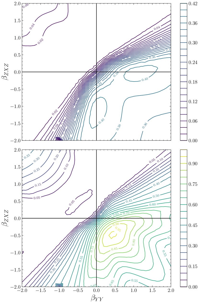
In the main text, we consider the preparation of GHZ states in the short-range model using two extra control Hamiltonians: and . Here we briefly analyze the optimal directions in this extra control space. We have the following annealing problem:
In Figure 6, we show a contour plot of the final fidelity for different combinations of and using local CD driving with and as defined in Eq. (4) for the Hamiltonian above with . We find that for the optimal protocol is very close to one where only one of the controls is used, i.e. where either or . The situation reverses for , where the optimal performance is achieved for . Figure 3 in the main text shows the protocol performance along the corresponding optimal directions.
Appendix C Details of the Method
In this section, we will describe in detail the step-by-step process by which we find these improved paths for local CD driving (see also Ref. Čepaitė et al., 2023). The first step is to determine the Hamiltonian for the physical system of interest, and represent it as a matrix. Furthermore, it is useful to leverage any symmetries present in the system and so construct the Hamiltonian in the relevant symmetry sector. This will make the local CD driving more efficient by reducing the number of transitions it tries to suppress. In the language of Eq. (5), this means determining in or and then forming
This corresponds to the red path in Figure 1. The next step is to “augment” this Hamiltonian by adding to it two extra control Hamiltonians, taking:
where and are defined as in Eq. (10). This corresponds to the blue path in Figure 1. We highlight that this is only the simplest possible choice such that the extra control Hamiltonians have no effect at the beginning () and end () of the protocol, and that we can even further improve the state preparation fidelity by taking further harmonics, i.e. taking at the price of introducing more variational parameters. More sophisticated methods such as quantum optimal control might also be employed for even further improvement.
The next step is perform local counterdiabatic driving. Using the “augmented” Hamiltonian in the Liouvillian , we construct the approximate AGP using the procedure outlined in Section A of this Appendix. We add this operator to form
With this local CD protocol , one can used standard numerical algorithms to solve the time-dependent Schrödinger equation to find the final state . By we mean that the final state will depend on the variational parameters of the extra controls Hamiltonians.
In this paper, we are working far from the adiabatic limit, so as long as , the precise way that the time-dependence is encoded in does not matter. However, for completeness we mention that we use a protocol which vanishes smoothly at and :
We then compute the fidelity using Eq. (8). We employ the Powell minimization algorithm Powell (1964) to choose the values of and which maximize the fidelity. Practically, we limit the values the coefficients can take to . This concludes the steps to implementing our protocol. In Figure 7 we apply this procedure to the short-range model Hamiltonian of Eq. (9).
We note that this algorithm finds local, not global, minima. So while it works well for a single harmonic per extra control term, the optimization becomes more difficult for further harmonics, and a global minimizer may be required. This could be due to glassiness in the landscape of possible control protocols Day et al. (2019).
Appendix D Explanation of Different Regimes of Fidelity Improvement
As remarked upon in the main text, in Figures 3, 4 and 7, we see two types of behavior for the fidelity of the final state prepared with extra control Hamiltonians. The first regime is a plateau where we can prepare the final state with near unit fidelity up to a certain system size, whereas the second regime has less than unit fidelity but is still exponentially improved when compared to the “naive” path.
To try to understand these, we refer to Ref. Claeys et al., 2019, where the variational optimization of the commutator ansatz for the AGP (Eq. (4) in this work) can be understood as simple polynomial fitting. We will summarize it here:
The exact matrix elements of the AGP in the energy eigenbasis satisfy
where we denote . We can write the matrix elements of the approximate AGP of Eq. (4) as
We define , where we have that
Thus, finding the approximate AGP can be thought of as finding the best approximation to by a fixed number of odd polynomials. This fitting procedure is nicely illustrated in Figure 1 of Ref. Claeys et al., 2019. While this might seem at first glance to be a system-independent problem, it depends strongly on the range of excitation frequencies which are present in the system.
We can imagine that in a system with very few independent excitation frequencies, the approximate AGP converges very quickly due to needing to fit at only a small number of points. This is exactly what happens for small system sizes, corresponding to the unit fidelity plateaus.
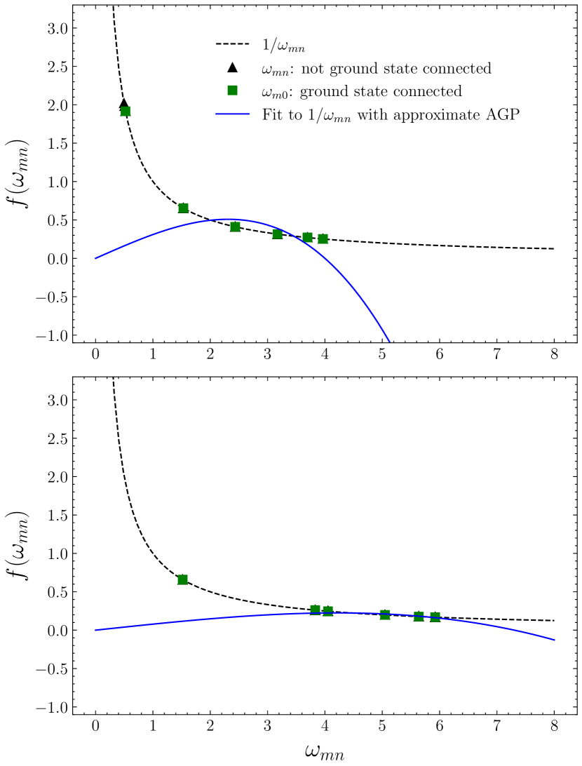
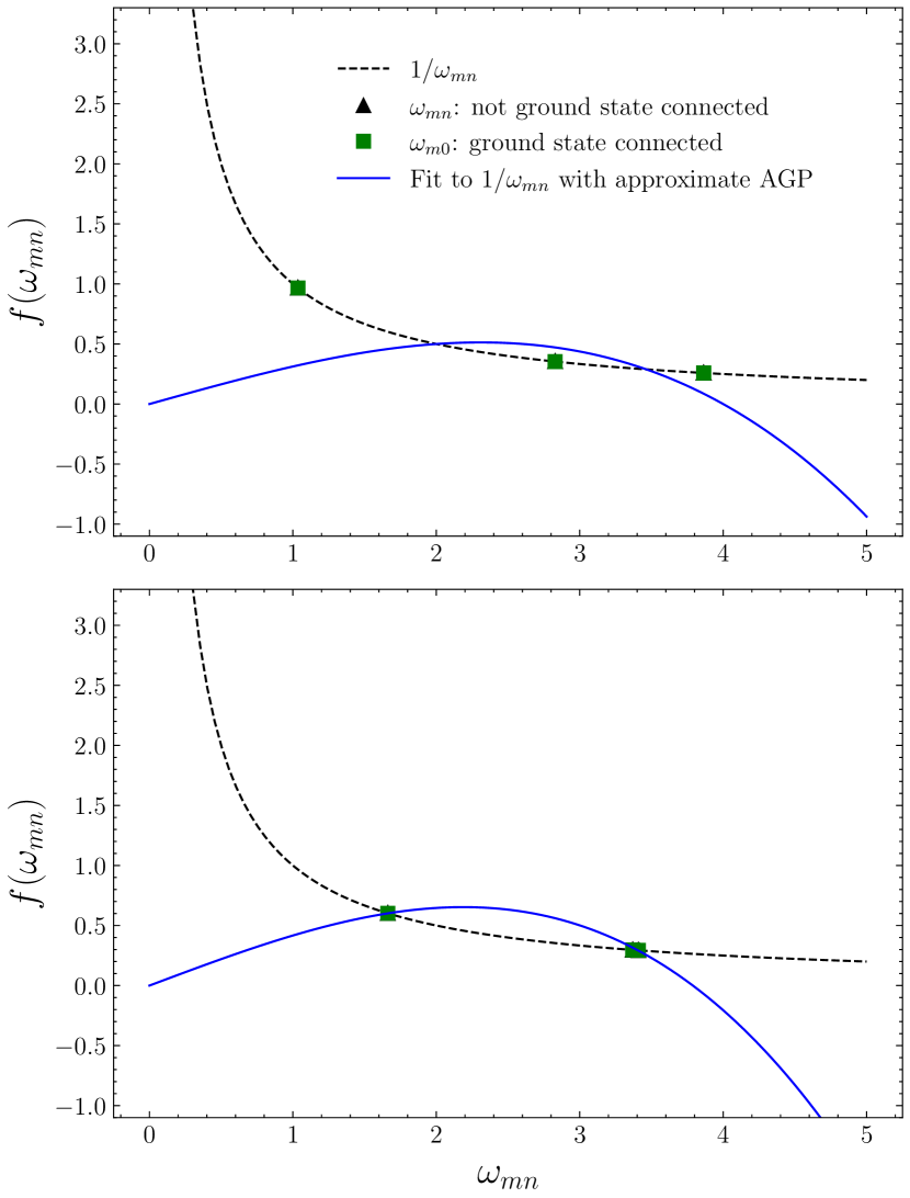
This fitting procedure happens for every point in the protocol. As an illustration we analyze here the point corresponding to , where the short-range model has a phase transition in the thermodynamic limit. In Figure 8, we show the polynomial obtained for the short-range model with using the variational procedure together with the exact result using . Crucially, we plot only the transition frequencies corresponding to the excitations from the ground state, which we denote by , which have nonzero matrix element . This significantly reduces the number of relevant frequencies compared to the Hilbert space size. The number of points is further reduced because there are many nearly degenerate transition frequencies. As a result the AGP is only required to suppress a small number of transitions, and hence a small number of points to fit to a polynomial.
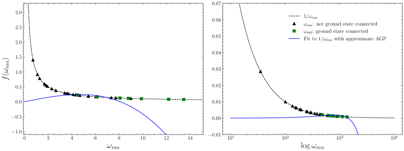
It is apparent that the extra control Hamiltonian fulfills two tasks: i) it increases the gap in the system and ii) it leads to clustering of states such that there are fewer different frequencies and thus it is easier to fit with low-order polynomials. For larger system sizes, the extra control Hamiltonian cannot group the independent excitation frequencies into just two “clumps,” so instead it pushes them to larger values, which is much easier to fit. This is shown in the case of in Figure 9, again with .
The short range Hamiltonian with the control is integrable and one might wonder if this fact allows for such efficiency of the polynomial fitting. This is, however, not the case and a very similar picture holds for nonintegrable models as well. In Figure 10 we show the long-range model with . Although there are now far more excited states which are connected to the ground state directly by , qualitatively the effect of the extra control Hamiltonian is similar: it pushes frequencies to higher values and clusters them together.