Constraining $z\lesssim 2$ ultraviolet emission with the upcoming ULTRASAT satellite

Abstract

The extragalactic background light (EBL) carries a huge astrophysical and cosmological content: its frequency spectrum and redshift evolution are determined by the integrated emission of unresolved sources, these being galaxies, active galactic nuclei, or more exotic components. The near-UV region of the EBL spectrum is currently not well constrained, yet a significant improvement can be expected thanks to the soon-to-be launched Ultraviolet Transient Astronomy Satellite (ULTRASAT). Intended to study transient events in the 2300-2900 $\rm\AA$ observed band, this detector will provide a reference full-sky map tracing the UV intensity fluctuations on the largest scales. In this paper, we suggest how to exploit its data in order to reconstruct the redshift evolution of the UV-EBL volume emissivity. We build upon the work of Chiang et al. (2018), where the clustering-based redshift (CBR) technique was used to study diffuse light maps from GALEX . Their results showed the capability of the cross correlation between GALEX and SDSS spectroscopic catalogs in constraining the UV emissivity, highlighting how CBR is sensitive only to the extragalactic emissions, avoiding foregrounds and Galactic contributions. In our analysis, we introduce a framework to forecast the CBR constraining power when applied to ULTRASAT and GALEX in cross correlation with the 5-year DESI spectroscopic survey. We show that these will yield a strong improvement in the measurement of the UV-EBL volume emissivity. Specifically, for the $\lambda=1500\,{\rm\AA}$ non-ionizing continuum below $z\sim 2$, we forecast a $1\sigma$ uncertainty $\lesssim 25\%\,(8\%)$ with conservative (optimistic) bias priors. We finally discuss how these results will foster our understanding of UV-EBL models.

I Introduction

Across the whole electromagnetic spectrum, light from unresolved sources of astrophysical and cosmological origins overlaps, producing the so-called extragalactic background light (EBL). Such integrated emission is observed and constrained through different probes; reviews in Refs. Cooray:2016jrk ; Hill:2018trh describe the main features of the EBL and highlight the degree of accuracy reached in the various frequency bands. Some regimes have been widely analysed, e.g., the microwave band where the cosmic microwave background (CMB) is observed or the optical-infrared region that collects redshifted emission from stars. Other frequency bands, instead, are still largely unprobed: the near-ultraviolet (NUV) to far-ultraviolet (FUV) region is one of these. Between $\nu_{\rm obs}\sim 1-3\cdot 10^{6}\,{\rm GHz}$ ($\lambda_{\rm obs}\sim 3000-1000\,{\rm\AA}$) a lower EBL limit has been estimated both using the integrated light from galaxy number counts and through photometric measurements from the Voyager 1 and 2 missions Murthy:1999 ; Eldstein:2000 , Hubble Brown:2000uq ; Bernstein:2001sq and the Galaxy Evolution Explorer (GALEX, Martin:2004yr ; Morrissey:2007hv ) Murthy:2010vf , even if with large statistical and systematic errors Cooray:2016jrk . This lack of measurements is not only due to technological issues: extragalactic photons in this regime get mostly absorbed by neutral hydrogen in the intergalactic medium (IGM) and inside the Milky Way. Moreover, Galactic light in this part of the spectrum provides a strong foreground contribution.

The study of the UV background plays an important role in understanding structure formation and star formation history, as depicted e.g. in Refs. Madau:2014bja ; Bernstein:2001sq and references within. First of all, its spectral energy distribution provides an unbiased estimate of the energy produced by star formation. Moreover, the EBL can be used to study the chemical enrichment history of the Universe, the total baryon fraction in stars and the local mass density of metals. The background radiation in this frequency band is highly correlated with the one in the infrared range Sasseen:1995 ; Schiminovich:1999qb , which is consistent with an origin related with dust-scattered stellar radiation. The UV-EBL can also contain contributions of cosmological origin, such as black hole accretion in quasars and active galactic nuclei (AGN), direct-collapse black hole formation or decaying and annihilating dark matter (see e.g., Refs. Dwek:1998bk ; Bond:1985pc ; Yue:2012dd ; Henry:2014jga ; Creque-Sarbinowski:2018ebl ; Bernal:2020lkd ).

Improving our knowledge of the UV-EBL is therefore a goal that should be pursued with upcoming instruments and surveys. In this context, a very interesting opportunity will soon be offered by the Ultraviolet Transient Astronomy Satellite (ULTRASAT, Sagiv:2013rma ; ULTRASAT:2022 ; Shvartzvald:2023ofi ), whose launch is scheduled for 2026. ULTRASAT foresees as its primary goal the study of astrophysical transients in the NUV band. In order to achieve this, part of the first six months of the mission will be dedicated to the realization of a full sky map, to be used as a reference frame for subsequent observations. Such map will reach a limiting AB magnitude of 23.5, thus providing a $\sim 10$ times sensitivity improvement with respect to the currently existing benchmark, namely the diffuse UV light map constructed in Ref. Murthy:2014 . This work used data from the All Sky and Medium Imaging Surveys performed by GALEX, masking resolved sources and binning pixels in order to estimate the combined contribution of the UV-EBL Sujatha:2009 ; Sujatha:2010fd and foregrounds, these being sourced by Galactic dust-scatter light, near-Earth airglow, or other Hamden:2013 ; Murthy:2013 ; Henry:2014jga ; Akshaya:2018 ; the origin of part of the foreground is yet unidentified. The GALEX map provided important results on the study of dust scattering emissions (e.g., Murthy:2016 ; Chiang:2019 ), correlation between UV and IR emissions (e.g., Murthy:2014 ; Saikia:2017 ), and extragalactic sources (e.g., Welch:2020 ; Chiang:2018miw ). The frequencies probed by GALEX allowed to access the UV-EBL between redshifts $z\!\sim\!0-1.5$; ULTRASAT will allow us to improve the sensitivity around $z\sim 1$, pushing the observations towards slightly higher $z$.

An innovative application has been presented by the authors of Ref. Chiang:2018miw ( C19 throughout this paper). UV satellites as GALEX and ULTRASAT observe a wide frequency range; therefore, radiation with various rest frame wavelengths, emitted at different cosmological distances from the observer, can be redshifted inside their observational band. The redshift dependence of the integrated, observed emission can be reconstructed through broadband tomography, which is based on the cross correlation between UV data and spectroscopic galaxy samples. This technique, also referred to as clustering based redshift (CBR), was originally developed in Refs. Newman:2008mb ; McQuinn:2013ib ; Menard:2013aaa , and applied in different contexts, e.g., to obtain a statistic estimate of the redshift of photometric samples Rahman:2014lfa ; Scottez:2016fju ; Morrison:2016stl ; DES:2017rfw , to study the cosmic infrared background Schmidt:2014jja , or the presence of extragalactic sources in Galactic dust maps Chiang:2019 , and to improve the constraining power of radio surveys on cosmological parameters Kovetz:2016hgp ; Scelfo:2021fqe . C19 applied this technique to the GALEX map, using catalogues from the Sloan Digital Sky Survey (SDSS, SDSS:2004dnq ; Reid:2015gra ), to reconstruct the redshift evolution of the UV-EBL volume emissivity. A follow-up of this work was realized in Ref. Scott:2021zue ( S21 in the paper), where the authors applied a similar formalism to forecast the constraining power of the Cosmological Advanced Survey Telescope for Optical and UV Research (CASTOR, Cote:2019 ) in cross correlation with Spectro-Photometer for the History of the Universe, Epoch of Reionization and Ices Explorer (SPHEREx, SPHEREx:2014bgr ; SPHEREx:2016vbo ; SPHEREx:2018xfm ).

The goal of our work is to build on the C19 analysis, applying it to the forecasted capabilities of ULTRASAT in cross correlation with upcoming spectroscopic galaxy surveys, in particular the Dark Energy Spectroscopic Instrument (DESI, DESI:2013agm ; DESI:2016fyo ; DESI:2016igz ). When the full release of DESI data will be available, it will also be possible to cross correlate its spectroscopic catalogs with the GALEX map from Ref. Murthy:2014 , and further improve the results from C19. In our analysis, therefore, we also consider the possibility of combining together GALEX and ULTRASAT maps with DESI, to perform a powerful CBR analysis, to access the UV-EBL particularly around $z\sim 1$.

Our paper is structured as follows. We begin in Sec. II by presenting the ULTRASAT satellite and giving some information about its specifications, in particular with respect to the construction of the full-sky map and the estimate of its noise. The approach we follow is inspired by line-intensity mapping science (see e.g., Refs. Kovetz:2017agg ; Bernal:2022jap for review). We proceed in Sec. III by modeling the signal that we aim to constrain, namely the UV volume emissivity (III.1). We then build the observable of interest in the context of the CBR technique, i.e., the angular cross correlation between an intensity map and a spectroscopic galaxy survey (III.2 and III.3), for which we also provide a noise estimate (III.4). Sec. IV presents our forecast analysis and collects our results. In particular, we start by reproducing the C19 constraints for GALEX$\times$SDSS (IV.2), and then we proceed by applying the technique to ULTRASAT$\times$DESI and (GALEX$+$ULTRASAT)$\times$DESI, comparing our forecasted results for the volume UV-EBL emissivity (IV.3) with various constraints available in the literature. We show that this approach will yield a strong improvement in the measurement of the UV-EBL volume emissivity. Our conclusions are presented and discussed in Sec. V.

II The ULTRASAT satellite

The observational window of ULTRASAT will span between $\lambda_{\rm min}=2300\,{\rm\AA}$ and $\lambda_{\rm max}=2900\,{\rm\AA}$, which implies an observed frequency range centered at $\nu_{\rm obs}=1.17\cdot 10^{6}\,{\rm GHz}$. To help understanding which redshift range can be mapped using these wavelengths, we consider the Lyman-$\alpha$ (Ly$\alpha$) line emission with rest frame $\lambda_{\rm Ly\alpha}=1216\,{\rm\AA}$: provided that $\lambda_{\rm obs}=\lambda_{\rm rest}(1+z)$, ULTRASAT will observe Ly$\alpha$ from $z_{\rm Ly\alpha}\in[0.9,1.4]$.

In our analysis in Sec. IV, we assume to rely on the UV map obtained during the first six month of the ULTRASAT mission. We assume that this will be realized using a technique similar to the one Ref. Murthy:2014 applied to GALEX data. The dataset we assume to analyse, hence consists of UV intensity values measured in the pixels of the map; the map is characterized by an intensity average value, which we also refer to as the monopole, and by spatial fluctuations; this indeed makes its study analogous to what is done in line-intensity mapping surveys Kovetz:2017agg ; Bernal:2022jap .

For both ULTRASAT and GALEX, the observed field is almost full-sky; the pixel scale is $5.4^{\prime\prime}/{\rm pix}$ for ULTRASAT, $5^{\prime\prime}/{\rm pix}$ for GALEX. The response function $R(\lambda_{\rm obs})$ of the instruments is defined in terms of the quantum efficiency, i.e., the number of electrons per incident photon depending on the frequency, normalized through

$$\int_{\lambda_{\rm obs}^{\rm min}}^{\lambda_{\rm obs}^{\rm max}}d\lambda_{\rm obs}\frac{R(\lambda_{\rm obs})}{\lambda_{\rm obs}}=1.$$ (1)

We compute the ULTRASAT response function based on information in Refs. Bastian_Querner_2021 ; Asif:2021vrm , and we show it in Fig. 1. Here, we also show $R(\lambda_{\rm obs})$ for the two GALEX filters, respectively centered in the NUV range $\lambda_{\rm obs}\in[1750,\,2800]\,{\rm\AA}$ and in the FUV range $\lambda_{\rm obs}\in[1350,\,1750]\,{\rm\AA}$. GALEX NUV filter observes Ly$\alpha$ in a similar range with respect to ULTRASAT, while GALEX FUV refers to a lower redshift regime, $z_{\rm Ly\alpha}\in[0.1,0.4]$. GALEX FUV and NUV filters, therefore, are complementary in probing Ly$\alpha$ emissions in the local Universe; ULTRASAT will improve the sensitivity mostly at $z\sim 1$.

The signal of interest for our analysis is modelled in the next section; here instead we provide an estimate of the noise variance in the maps. As C19 details, masking the pixels with flux above the detection limit, resolved sources can be separated from the diffuse light contribution. This separation on the map level helps to implement the algorithms required to mitigate the foreground noise; on the other hand, a combined analysis of the two components allows us to study the UV intensity field without selection effects. From now on, we thus assume that a procedure similar to C19 has been performed: resolved sources and diffuse light are initially separated to create the maps and estimate their noises, but they are then summed to perform the analysis.

The noise variance per pixel in the “overall” map is estimated based on the $5\sigma$ AB magnitude limit $m_{\rm AB}$, weighted by the different exposure times during the observations. In the case of GALEX NUV and FUV, C19 indicates $m_{\rm AB}\sim 20.5$ - $23.5$; we adopt the intermediate value $m_{\rm AB}=22$. For ULTRASAT reference map instead, following Ref. Shvartzvald:2023ofi , we assume $m_{\rm AB}=23.5$, so to get a $\times 10$ sensitivity improvement from GALEX.

The limiting magnitude characterizes the detection level above which sources (with Galactic or extragalactic origin) cannot be resolved; for this reason, we can use it to describe the ground level of the observed intensity inside a region with comparable size to the point spread function. We convert $m_{\rm AB}$ to flux per pixel via $m_{\rm AB}=8.90-2.5\log_{10}\mathcal{F}_{\nu}$, and we rescale it to flux density inside a certain angular region as $f_{\nu}^{\rm pix}=\mathcal{F}_{\nu}/A_{\rm pix}$. The pixel surface area is computed as $A_{\rm pix}=L_{\rm pix}^{2}$, where $L_{\rm pix}$ is the pixel scale. The value obtained corresponds to sources that are $5$ times brighter than the noise level; therefore, we get the total noise variance per pixel as

$$\sigma_{N}^{2}=\left[{f_{\nu}^{\rm pix}}/{5}\right]^{2}.$$ (2)

To reduce the value of $\sigma_{N}^{2}$, it is always possible to combine the pixels in groups, which we call “effective pixels”: this reduces their number, and it averages noise fluctuation on the smallest scales. We will discuss in Sec. III.4 that, in the context of the CBR analysis, C19 used effective pixels with $L_{\rm pix}^{\rm eff}=50\,^{\prime\prime}/{\rm pix}$; we will show that instead, ULTRASAT will obtain good results already using $L_{\rm pix}$. Note that, so far, we did not account for foreground contributions; these will be described in Sec. III.4.

Tab. 1 collects the main survey specifications we discussed so far, and it compares their estimated $\sigma_{N}^{2}$ value. The table also reports the value of the observed monopole $J_{\nu_{\rm obs}}$, which we define in Sec. III.2.

	$\lambda_{\rm obs}$	$z_{\rm Ly\alpha}$	$L_{\rm pix}^{\rm(eff)}$	$J_{\nu_{\rm obs}}$	$\sigma_{N}^{2}$
	[Å]		[“/px]	[Jy/sr]	[${\rm Jy^{2}/sr^{2}}$]
ULTRASAT	[2300, 2900]	[0.9, 1.4]	5.45	237	422
GALEX	[1350, 1750]	[0.1, 0.4]	5 (50)	264	1959
	[1750, ,2800]	[0.4, 1.3]	5 (50)	79	1959

Table 1: Specs of the broadband surveys ULTRASAT Shvartzvald:2023ofi and GALEX Martin:2004yr . The redshift range $z_{\rm Ly\alpha}$ is computed for the Ly$\alpha$ line $\lambda_{\rm Ly\alpha}=1216\,{\rm\AA}$; other parts of the UV spectrum are shifted to different ranges. We indicate both the pixel scale $L_{\rm pix}$ and (in parenthesis) the effective scale of the pixels used in the analysis in Sec. IV. The monopole $J_{\nu_{\rm obs}}$ and the variance $\sigma_{N}^{2}$ are estimated using respectively Eqs. (10) and (2).

III Modeling the signal and noise

The broadband measurements ULTRASAT will realize integrate the radiation emitted over a wide frequency and redshift range. Reconstructing the spectral shape of the signal, as well as its evolution across cosmic time, is of fundamental importance to disentangle cosmological dependencies and astrophysical properties of the emitters. One way this goal can be pursued is via the broadband tomography, or clustering-based redshift (CBR) technique Newman:2008mb ; McQuinn:2013ib ; Menard:2013aaa , namely the cross correlation between one broadband survey (ULTRASAT or GALEX, in our case) and a reference spectroscopic galaxy catalogue. Using cross correlations allows us to overcome the presence of Galactic foregrounds, ensuring that the measured signal has extragalactic origin. The possibility of chance correlation is further reduced by the fact that foregrounds fluctuate mainly at large scales, while we are interested in cross correlations on small scales. Hence, in our analysis, foregrounds only contribute to the noise budget.

The authors of C19 applied CBR to GALEX data, in order to constrain the redshift evolution of the UV-EBL volume emissivity. In their case, a subset of the SDSS catalogs SDSS:2004dnq ; Reid:2015gra was adopted as reference. ULTRASAT, with its improved NUV capability, seems to be the perfect heir for this kind of analysis. Considering its timeline, a bunch of state-of-the-art galaxy surveys will be available to perform the cross correlation. As we will detail in Sec. III.4, the best results are obtained for small spectroscopic redshift uncertainties and large galaxy number densities in the range under analysis. For this reason, we decided to rely on the DESI DESI:2013agm ; DESI:2016fyo ; DESI:2016igz forecasted 5 years capability, which are depicted in Ref. DESI:2023dwi .

To forecast the constraining power ULTRASAT$\times$DESI will have compared to GALEX$\times$SDSS, we introduce the quantities required to model the observables. In Sec. III.1, we follow the formalism from C19 and S21 and we describe the UV-EBL volume emissivity that we aim to constrain. The emissivity is then converted into observed intensity in Sec. III.2. We then review how CBR can reconstruct its redshift evolution in Sec. III.3, and we estimate the unceratinty in its measurement in Sec. III.4. Fig. 1 summarizes the logic and modeling of the analysis.

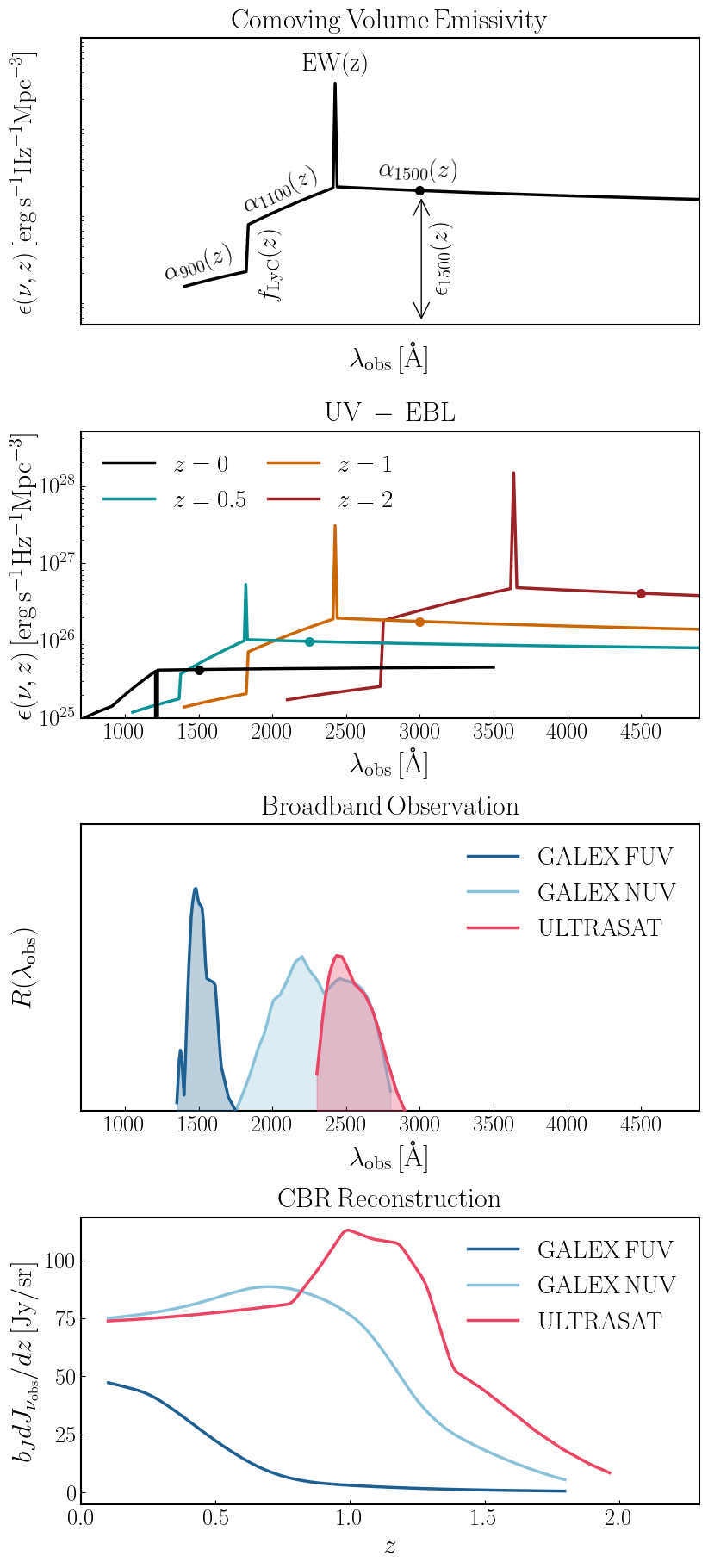
Figure 1: Summary of the modeling in our analysis. We characterize the UV volume emissivity $\epsilon(\nu,z)$ based on Eqs. (3) to (6) (panel 1). Emissions from different $z$ contribute to the EBL (panel 2, the dots show $\lambda_{\rm rest}=1500\,{\rm\AA}$; the Ly$\alpha$ line is in absorption at low $z$), which is weighted by the detector response function in the broadband observation in Eq. (10) (panel 3). The CBR allows us to reconstruct $b_{J}(z)dJ_{\nu_{\rm obs}}/dz$ in Eqs. (11), (13) (panel 4). Figure inspired by Ref. Chiang:2018miw .

III.1 UV volume emissivity

The first ingredient we need in order to model the signal is the spatially averaged comoving volume UV emissivity, $\epsilon(\nu,z)$ $[\rm erg\,s^{-1}Hz^{-1}Mpc^{-3}]$. In analogy to C19 and S21, we parameterize its frequency and redshift dependencies using a piecewise function, capable of describing the different spectral contributions the EBL receives. This model is in agreement with simulation results based on the study of the radiative transfer of Lyman continuum photons in the IGM Haardt:2011xv .

We distinguish between the non-ionizing continuum at $\lambda_{\rm rest}>1216\,{\rm\AA}$ and between $912{\,\rm\AA}<\lambda_{\rm rest}\leq 1216\,{\rm\AA}$, the Ly$\alpha$ line at $\lambda_{\rm rest}=1216\,{\rm\AA}$, and the ionizing continuum at $\lambda_{\rm rest}\leq 912\,{\rm\AA}$, below the Lyman break. Above Ly$\alpha$, we describe the frequency and redshift evolution of the non-ionizing continuum with respect to a pivot value as

$$\epsilon(\nu,z)=\epsilon_{1500}\left[\frac{\nu}{\nu_{1500}}\right]^{\alpha_{1500}},$$ (3)

where $\nu_{1500}$ is the frequency at $\lambda_{\rm rest}=1500\,$Å.

Between the Ly$\alpha$ line and the Lyman break, we adopt

$$\epsilon(\nu,z)=\epsilon_{1500}\left[\dfrac{\nu_{1216}}{\nu_{1500}}\right]^{\alpha_{1500}}\begin{cases}&\left[\dfrac{\nu}{\nu_{1216}}\right]^{\alpha_{1100}}\\ &\dfrac{{\rm EW}}{\nu_{1216}\delta}\dfrac{\nu^{2}}{c}+\left[\dfrac{\nu}{\nu_{1216}}\right]^{\alpha_{1100}}\end{cases}$$ (4)

where the first line holds for $|\nu-\nu_{1216}|>\nu_{1216}\delta$, with $\delta=0.005$ and line frequency $\nu_{1216}=2.5\times 10^{6}\,{\rm GHz}$. Finally, in the ionizing range we set

$$\epsilon(\nu,z)=\epsilon_{1500}\left[\frac{\nu_{1216}}{\nu_{1500}}\right]^{\alpha_{1500}}f_{\rm LyC}\left[\frac{\nu_{912}}{\nu_{1216}}\right]^{\alpha_{1100}}\left[\frac{\nu}{\nu_{912}}\right]^{\alpha_{900}}.$$ (5)

The redshift dependencies of Eqs. (3), (4), (5) are encapsulated in the normalization and slope parameters of the continuum, namely

$$\epsilon_{1500}=\epsilon_{1500}^{z=0}(1+z)^{\gamma_{1500}},$$ (6)

$$\alpha_{1500}=\alpha_{1500}^{z=0}+C_{1500}\log_{10}(1+z),$$

$$\alpha_{1100}=\alpha_{1100}^{z=0}+C_{1100}\log_{10}(1+z),$$

$$\alpha_{900}=\alpha_{900}^{z=0},$$

as well as in the line equivalent width,

$${\rm EW}=C_{\rm Ly\alpha}\log_{10}\left(\frac{1+z}{1+z_{\rm EW1}}\right)+{\rm EW}^{z=z_{\rm EW1}},$$ (7)

$$C_{\rm Ly\alpha}=\frac{{\rm EW}^{z=z_{\rm EW2}}-{\rm EW}^{z=z_{\rm EW1}}}{\log_{10}[(1+z_{\rm EW2})/(1+z_{\rm EW1})]}\,,$$

and in the Lyman continuum escape fraction in the IGM

$$\log_{10}f_{\rm LyC}=C_{\rm LyC}\log_{10}\left(\frac{1+z}{1+z_{\rm C1}}\right)+\log_{10}f_{\rm LyC}^{z=z_{\rm C1}}\,,$$ (8)

$$C_{\rm LyC}=\frac{\log_{10}f_{\rm LyC}^{z=z_{\rm C2}}-\log_{10}f_{\rm LyC}^{z=z_{\rm C1}}}{\log_{10}[(1+z_{\rm C2})/(1+z_{\rm C1})]}\,.$$

Overall, as Fig. 1 shows in the top panel, the amplitude of the volume emissivity is set by $\epsilon_{1500}(z)$, while the characterisitics of the Ly$\alpha$ line are determined by ${\rm EW}(z)$, and the amplitude of the Lyman break by $f_{\rm LyC}(z)$. At each $z$, the $\alpha_{l}(z)$ parameters $(l=1500,1100,900)$ set the slopes of the frequency dependence in the different regimes.

The upper part of Tab. 2 collects the parameters through which we parameterize the volume emissivity $\epsilon(\nu,z)$, together with their fiducial values according to C19. To analyse both the GALEX NUV and FUV filters, C19 sets the pivot points of the EW in Eq. (7) to $\{z_{\rm EW1}=0.3,\,z_{\rm EW2}=1\}$, and the ones of the escape fraction in Eq. (8) to $\{z_{\rm C1}=1,\,z_{\rm C2}=2\}$. In our ULTRASAT analysis, we decided to keep the same pivot points for the escape fraction, while we pivoted the EW at $\{z_{\rm EW1}=1,\,z_{\rm EW2}=2\}$: the higher redshift has been chosen according to the ULTRASAT $\lambda_{\rm obs}$ regime, which collects emissions from the Ly$\alpha$ line at $z_{\rm Ly\alpha}\in[0.9,\,1.4]$ (compare with Tab. 1) and from the Lyman break at $z_{912}\in[1.5,\,2.2]$. To get a continuous signal, we estimated the value of ${\rm EW}^{z=2}$ from Eq. (7), using the C19 pivots points. Fig. 1 shows $\epsilon(\nu,z)$ at different $z$.

Parameter	Fiducial value	Parameter	Fiducial value
$\log_{10}\epsilon_{1500}^{z=0}$	25.63	$\gamma_{1500}$	2.06
$\alpha_{1500}^{z=0}$	-0.08	$C_{1500}$	1.85
$\alpha_{1100}^{z=0}$	-3.71	$C_{1100}$	0.50
$\alpha_{900}^{z=0}$	-1.5	${\rm EW}^{z=0.3}$	-6.17 Å
${\rm EW}^{z=1}$	88.02 Å	${\rm EW}^{z=2}$	176.7 Å
$\log_{10}f_{\rm LyC}^{z=1}$	-0.53	$\log_{10}f_{\rm LyC}^{z=2}$	-0.84
$b_{1500}^{z=0}$	0.32	$\gamma_{\nu}$	-0.86
$\log_{10}[\epsilon b]_{1500}^{z=0}$	25.62	$\gamma_{z}$	0.79

Table 2: Parameters to model the emissivity $\epsilon(\nu,z)$ in Eqs. (3), (4), (5) and the bias in Eq. (12); in the analysis in Sec. IV, we use the parameter $\log_{10}[\epsilon b]_{1500}^{z=0}$ to collect the degeneracy between $\epsilon_{1500}^{z=0}$ and $b_{1500}^{z=0}$. Values from Ref. Chiang:2018miw .

III.2 Observed intensity

The volume emissivity we modelled so far describes the UV emission at the source; broadband observations, however, have to deal with a combination of effects to convert this quantity into the observed, integrated, specific intensity $J_{\nu_{\rm obs}}\,[{\rm Jy/sr}]$.

First of all, the presence of HI clumps along the line-of-sight partially absorbs the UV radiation before it is observed. The effective optical depth $\tau(z)$ of this phenomenon has been originally estimated in Ref. Madau:1995js , accounting for a Poisson distribution of the absorbers as a function of their column density and redshift. Absorption is efficient for radiation with $\lambda_{\rm rest}$ either smaller than the ionization wavelength 912 Å  or comparable with Ly$\alpha$ and other lines in the Lyman series, which give rise to the Lyman forest Gunn:1965 ; Steidel:1987 ; Madau:1995js . In our analysis, we rely on the improved semi-analytical model in Ref. Inoue:2014zna , described by a piecewise power-law in overall agreement with Ref. Madau:1995js .

The UV volume emissivity in our computation hence is given by $\epsilon(\nu,z)e^{-\tau(\nu)}$, where $\tau(\nu)$ is the optical depth. By using the radiative transfer function in an expanding Universe, it is possible to convert this quantity into specific intensity Gnedin:1996qr , through

$$j(\nu_{\rm obs})=\frac{c}{4\pi}\int_{0}^{\infty}\frac{dz}{H(z)(1+z)}\,\epsilon(\nu,z)\,e^{-\tau(\nu)}.$$ (9)

where $\nu_{\rm obs}=\nu/(1+z)$, $c$ is the speed of light and $H(z)$ the Hubble factor. In a broadband survey, such as ULTRASAT or GALEX, observations are performed over a wide range of frequencies, weighted by the detector response function. The observed monopole, hence, is

$${J}_{\nu_{\rm obs}}=\int_{\nu_{\rm obs}^{\rm min}}^{\nu_{\rm obs}^{\rm max}}\frac{d\nu_{\rm obs}}{\nu_{\rm obs}}\,j(\nu_{\rm obs}){R}(\nu_{\rm obs})\,,$$ (10)

where $R(\nu_{\rm obs})$ is the quantity in Eq. (1) once the wavelength is converted into frequency. We estimate ${J}_{\nu_{\rm obs}}=237\,{\rm Jy/sr}$ for ULTRASAT, while ${J}_{\nu_{\rm obs}}=264\,{\rm Jy/sr},\,79\,{\rm Jy/sr}$ for GALEX NUV and FUV respectively, in agreement with measurements presented in C19.

Our modeling of $J_{\nu_{\rm obs}}$ only accounts for extragalactic contributions, while real data include foregrounds. As we will discuss in the next section, the CBR technique generally provides an unbiased estimator of the extragalactic radiation field, which overcomes the foreground problem. At this stage, we can thus safely rely on a signal model that only contains extragalactic UV contributions, and include the foregrounds only in the noise budget.

III.3 Spectral tagging via clustering-based redshifts

The band-averaged specific intensity in Eq. (10) contains the integrated information about the redshift evolution of the UV volume emissivity. The CBR technique Newman:2008mb ; McQuinn:2013ib ; Menard:2013aaa offers a possible way to reconstruct the redshift dependenc $dJ_{\nu_{\rm obs}}/dz$, based on the correlation between the broadband survey and the spectroscopic galaxy catalog that is used as reference sample.

On one side, the specific intensities $J_{\nu_{\rm obs}}$ measured in the pixels of the broadband map provide a dataset with unknown redshifts, whose spatial fluctuations are determined by the way UV emitters trace the underlying large-scale structure (LSS). On the other side, galaxies in the spectroscopic sample trace the LSS as well, and they can be divided in consecutive slices of well-known redshift. The angular cross correlation between the two datasets can then be exploited to remap $J_{\nu_{\rm obs}}$ in terms of the redshift-dependent specific intensity

$$\frac{dJ_{\nu}(z)}{dz}= \frac{c}{4\pi H(z)(1+z)}\,\,\times$$ (11)

$$\times\int_{\nu_{\rm obs}^{\rm min}}^{\nu_{\rm obs}^{\rm max}}\frac{d\nu_{\rm obs}}{\nu_{\rm obs}}R(\nu_{\rm obs})\epsilon(\nu,z)e^{-\tau(\nu_{\rm obs},z)}\,.$$

The amplitude of the correlation, in fact, will peak for intensity-galaxy pairs who trace the LSS in a common redshift range. As C19 shows, this quantity can be constructed by using the absolute value of the intensity, namely including foregrounds and Galactic emmissions; even if this is the case, the cross correlation is capable of isolating the extragalactic contribution.

The measurement obtained with CBR, however, will be degenerate with the bias of the sources of the unknown-redshift sample, namely the UV emitters; following C19 and S21, we parametrize it as

$$b(\nu,z)=b_{1500}^{z=0}\left[\frac{\nu}{\nu_{1500}}\right]^{\gamma_{b_{\nu}}}(1+z)^{\gamma_{b_{z}}},$$ (12)

where we normalized the frequency dependence to the value at 1500 Å, analogously to the other parameters used to model the emissivity in Sec. III.1; fiducial values are collected in Tab. 2. The value of $b_{1500}^{z=0}$ is degenerate with $\epsilon_{1500}^{z=0}$ in determining the amplitude of the signal, as will become evident in the following.

In the data of the UV broadband survey, the information on the clustering enters through an effective intensity-weighted bias $b_{J}(z)$, which is computed from the source bias in Eq. (12) through

$$b_{J}(z)=\frac{\int_{\nu_{\rm obs}^{\rm min}}^{\nu_{\rm obs}^{\rm max}}{d\nu_{\rm obs}}{\nu_{\rm obs}^{-1}}\,{R}(\nu_{\rm obs})\,b(\nu,z)\epsilon(\nu,z)\,e^{-\tau(\nu)}}{\int_{\nu_{\rm obs}^{\rm min}}^{\nu_{\rm obs}^{\rm max}}{d\nu_{\rm obs}}{\nu_{\rm obs}^{-1}}\,{R}(\nu_{\rm obs})\epsilon(\nu,z)\,e^{-\tau(\nu)}}.$$ (13)

To model the CBR observable, we start by defining the fluctuations in the map measurements in terms of the angular position $\phi$ as

$$\Delta J_{\nu_{\rm obs}}(\phi)=J_{\nu_{\rm obs}}(\phi)-\langle J_{\nu_{\rm obs}}\rangle,$$ (14)

where $\langle J_{\nu_{\rm obs}}\rangle$ is the ensamble average. The galaxy survey, instead, is used to trace the 3D overdensity field through

$$\delta_{g}(\phi,z)=\frac{n_{g}(\phi,z)-\langle n_{g}(z)\rangle}{\langle n_{g}(z)\rangle}=b_{g}(z)\delta_{m}(\phi,z),$$ (15)

where $n_{g}(\phi,z)$ is the galaxy number density, $b_{g}(z)$ the galaxy bias and $\delta_{m}(\phi,z)$ describes the LSS overdensities in the underlying dark matter (DM) field.

The choice of the reference galaxy survey depends on the redshift range and precision one wants to achieve. C19 uses SDSS data from Refs. SDSS:2004dnq ; Reid:2015gra , while we decided to adopt the forecasts for the 5-year results of DESI, described in Ref. DESI:2023dwi . As Tab. 3 shows, both surveys provide catalogs mapping different kind of sources; Fig. 2 shows the number of galaxies they contain in each redshift bin, namely

$$N_{g,i}=\Delta z_{i}\Omega_{\rm survey}\frac{dN_{g}}{dzd\Omega}\,,$$ (16)

where $dN_{g}/dzd\Omega$ is the number of galaxies per steradian per redshift bin, $\Omega_{\rm survey}$ is the sky area observed by the survey, and $\Delta z_{i}$ the width of the bin.

	$N_{g}$	$\delta z_{i}$	$\Delta z_{i}$	catalog	$z$
DESI	$\mathcal{O}(10^{7})$	0.0005	0.1	BGS	[0.1, 0.4]
				LRG	[0.4, 1.1]
				ELG	[1.1, 1.6]
				QSO	[1.6, 2]
SDSS	$\mathcal{O}(10^{5})$	0.003	0.1	NYU MAIN	[0.1, 0.2]
				BOSS LOWZ	[0.1, 0.4]
				BOSS CMASS	[0.4, 0.7]
				DR14 QSO	[0.7, 2]

Table 3: Specs of the galaxy surveys (DESI DESI:2023dwi and SDSS SDSS:2004dnq ; Reid:2015gra ) considered in this work. The forecasted sources in DESI are divided between bright galaxies (BGS), luminous red galaxies (LRG), emission line galaxies (ELG) and quasars (QSO); SDSS instead contains results from the galaxy NYU value-added catalog, the luminous red galaxy samples in BOSS and the quasars in the DR14 release. The total number $N_{g}$ is obtained by integrating $dN_{g}/dzd\Omega$ over the redshift and observed sky area. $\delta z_{i}$ and $\Delta z_{i}$ describe respectively the width of the spectroscopic bins and the width of the redshift bins used in our forecast analysis, see Sec. III.4.

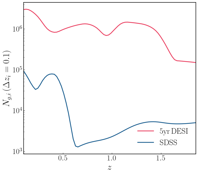
Figure 2: Number of galaxies per redshift bin with size $\Delta z=0.1$; values for DESI are from Ref. DESI:2023dwi , while SDSS from Refs. SDSS:2004dnq ; Reid:2015gra . Discontinuities are due to different catalogs.

The angular cross correlation between intensity pixels and galaxies that are separated by an angle $\theta$ on the sky is finally defined as

$$\omega_{Jg}(\theta,z)=\langle\Delta J_{\nu_{\rm obs}}(\phi)\delta_{g}(\phi,z)\rangle,$$ (17)

and then marginalized over $\theta$ in order to get

$$\bar{\omega}_{Jg}(z)=\int_{\theta_{\rm min}}^{\theta_{\rm max}}d\theta\,W(\theta)\omega_{Jg}(\theta,z)\,.$$ (18)

This is the main observable we are interested in for our analysis. The choice of the window function $W(\theta)$ is arbitrary; in analogy with C19 and S21, we choose $W(\theta)=\theta^{-0.8}/\int\theta^{-0.8}d\theta$. The minimum angular distance above which the cross correlation is performed, is set to $\theta_{\rm min}(z)=\arctan[r_{\rm min}/D_{A}(z)]$, where $D_{A}(z)$ is the cosmological angular diameter distance and $r_{\rm min}=0.5\,{\rm Mpc}$ is a physical scale chosen to avoid strong non-linear clustering on small scales. For $z\in[0.1,2]$ we get $\theta_{\rm min}\in[4,0.97]\,{\rm arcmin}$, larger than $L_{\rm pix}$ in Tab. 1. The choice of $\theta_{\rm max}$, instead, is set to avoid large fluctuations in the calibration of the map. In our case, ULTRASAT has a wide field-of-view (FoV) $\Omega_{\rm Fov}=204\,{\rm deg}^{2}$, across which observational properties vary. Ref. Shvartzvald:2023ofi shows that the effective PSF is almost constant up to $\sim 4\,{\rm deg}$ from the center of the FoV; therefore, we assume that inside this range calibrations are stable and we run our analysis up to $\theta_{\rm max}=4\,{\rm deg}$. In the case of GALEX, instead, C19 chooses $\theta_{\rm max}(z)=\arctan[5{\,\rm Mpc}/D_{A}(z)]\in[44,10]\,{\rm arcmin}=[0.7,0.2]\,{\rm deg}$. We adopt the same value when dealing with GALEX in our analysis.

The angular cross correlation $\bar{\omega}_{\tilde{J}{\rm g}}(z)$ defined in Eq. (18) represents the CBR observable, and can then be used to infer the redshift evolution of the specific intensity. In fact, we can re-express it as

$$\bar{\omega}_{\tilde{J}{\rm g}}(z)=b_{J}(z)b_{g}(z)\frac{dJ_{\nu_{\rm obs}}}{dz}\int_{\theta_{\rm min}(z)}^{\theta_{\rm max}(z)}d\theta\,W(\theta)\omega_{m}(\theta,z),$$ (19)

where $b_{J}(z)$ and $b_{g}(z)$ are the biases of the two LSS tracers, and $\omega_{m}(\theta,z)$ is the angular two-point function of the underlying DM field. This can be related to the non-linear matter power spectrum Maller:2003eg via

$$\omega_{m}(\theta,z)=\frac{1}{2\pi}\int_{0}^{\infty}dk\,kP_{m}(k,z)\mathcal{J}_{0}(k\theta\chi(z))\frac{dz}{d\chi},$$ (20)

where $\mathcal{J}_{0}$ is the Bessel function of the first type, $\chi(z)$ the radial comoving distance and $dz/d\chi=H(z)/c$.

The observation of $\bar{\omega}_{\tilde{J}{\rm g}}(z)$ then leads to the reconstruction of the redshift evolution of the intensity weighted by the bias, $d\tilde{J}_{\nu_{\rm obs}}/dz=b_{J}(z)dJ_{\nu_{\rm obs}}/dz$. This in turn represents a summary statistics of the UV emission and absorption across space and time. We show $d\tilde{J}_{\nu_{\rm obs}}/dz$ in Fig. 1, for ULTRASAT and GALEX (NUV, FUV), while Fig. 3 shows the CBR signal-to-noise ratio of $\bar{\omega}_{\tilde{J}{\rm g}}(z)$ when their maps are cross correlated with the galaxy reference catalogs from SDSS or DESI. These are the quantities that enter our analysis in Sec. IV.

III.4 Noise

Refs. Newman:2008mb ; Menard:2013aaa estimate analytically the uncertainty on the CBR angular cross correlation $\bar{\omega}_{\tilde{J}{\rm g}}(z)$ introduced in Eq. (19). We follow a similar reasoning to they do, accounting for the fact that the broadband UV data are measured as intensity in pixels rather than point sources, as is done instead in photometric galaxy surveys.

In the broadband survey, we model the monopole in each pixel by summing the EBL from Eq. (10) with an estimate of the foreground. This provides an offset between the expected and observed $J_{\nu_{\rm obs}}$, that has indeed been observed. The authors of Ref. Akshaya:2018 estimated the observed surface brightness in photon units to be $\sim 250\,{\rm ph\,cm^{-2}s^{-1}sr^{-1}\AA^{-1}}$ in the FUV band, and $\sim 550\,{\rm ph\,cm^{-2}s^{-1}sr^{-1}\AA^{-1}}$ in the NUV band. C19 explains the offset as due to the presence of three main foregrounds: near-Earth airglow and zodiacal light (the latter being relevant only in the NUV band, see Ref. Murthy:2013 ), Galactic dust, and a component whose origin is unknown. We account for all these sources adding to the EBL monopole a fractional contribution $\mathcal{A}_{\rm fg}J_{\nu_{\rm obs}}$, so that $J_{\nu}^{\rm obs}=J_{\nu_{\rm obs}}(1+\mathcal{A}_{\rm fg})$. We set $\mathcal{A}_{\rm fg}=1.8$ for GALEX FUV and $2.2$ for GALEX NUV and ULTRASAT, since they observe similar bands. We assume data are Poisson-distributed over pixels (thus we estimate the variance as the signal mean value), while fluctuations are Gaussian with variance $\sigma_{N}^{2}$ from Eq. (2); the total noise hence is

$$\sigma_{J}^{2}=[J_{\nu_{\rm obs}}(1+\mathcal{A}_{\rm fg})]^{2}+\sigma_{N}^{2}.$$ (21)

As described in Sec. III.3, the CBR cross correlation is computed in patches of area $\pi\theta_{\rm max}^{2}$, where $\theta_{\rm max}=4\,{\rm deg}$ for ULTRASAT and $\theta_{\rm max}\sim[0.7,\,0.2]\,{\rm deg}$ for GALEX. Therefore, to infer the noise we need to account for all the possible pairs of pixels and reference galaxies per redshift bin that can be created inside the patches. We rescale the total number of pixels $N_{\rm pix}^{\rm tot}$ inside $\pi\theta_{\rm max}^{2}$ as

$$N_{\rm pix}=N_{\rm pix}^{\rm tot}{\pi\theta_{\rm max}^{2}}/{\Omega_{\rm sky}}={\pi\theta_{\rm max}^{2}}/{A_{\rm pix}},$$ (22)

where we used $N_{\rm pix}^{\rm tot}=\Omega_{\rm sky}/A_{\rm pix}$, $\Omega_{\rm sky}$ being the sky area observed by the broadband survey, while $A_{\rm pix}=L_{\rm pix}^{2}$ the area of the pixels computed using Tab. 1. Meanwhile, the number of galaxies per $z$ bin in the same area is

$$N_{g,i}^{\theta_{\rm max}}=\frac{dN_{g}}{dzd\Omega}{\Delta z_{i}\pi\theta_{\rm max}^{2}}=N_{g,i}\frac{\pi\theta_{\rm max}^{2}}{\Omega_{\rm survey}},$$ (23)

where $N_{g,i}=\Delta z_{i}\Omega_{\rm survey}dN_{\rm g}/dzd\Omega$ is the number of reference galaxies in the observed area of the survey $\Omega_{\rm survey}$ in the $i$-th redshift bin having size $\Delta z_{i}$ (see Fig. 2).

Finally, we estimate the number of pairs to be

$$N_{\rm pairs}=N_{\rm pix}N_{g,i}^{\theta_{\rm max}}=\frac{N_{g,i}}{A_{\rm pix}}\frac{(\pi\theta_{\rm max}^{2})^{2}}{\Omega_{\rm survey}}\,.$$ (24)

In the case of ULTRASAT$\times$DESI and GALEX$\times$DESI, the observed sky area is set by the galaxy survey, namely $\Omega_{\rm survey}=14000\,{\rm deg}^{2}$ DESI:2023dwi ; following the procedure in C19, instead, for GALEX$\times$SDSS we set $\Omega_{\rm survey}=5500\,{\rm deg^{2}}$, which is the size of the overlapping footprints. In analogy to S21 and Ref. Chiang:2019 , for SDSS we set $\Delta z_{i}=0.1$, hence we sample the $[0,2]$ redshift range with 20 bins. This width is larger than the uncertainty of the spectroscopic redshift bins $\delta z_{i}$: in fact, as it has been shown in Refs. Menard:2013aaa ; Rahman:2014lfa , CBR provides a measurement of the redshift which is degenerate with the bias evolution in $z$. This degrades the goodness of the CBR-redshift inference, and it can lead to the overlap between contiguous bins when their width is too small. In the case of SDSS, the width $\Delta z_{i}=0.1$ allows us to overcome this issue; in the case of DESI, we make the conservative choice of using the same redshift bin width.

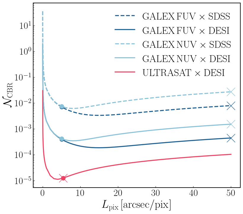
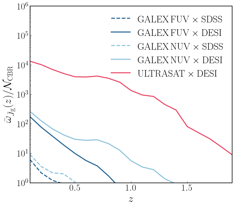
Figure 3: Noise analysis for ULTRASAT$\times$DESI (pink), GALEX NUV$\times$SDSS and $\times$DESI (light blue, dashed and continuous) and GALEX FUV$\times$SDSS and $\times$DESI (dark blue, dashed and continuous). Left: $\mathcal{N}_{\rm CBR}$ from Eq. (25). Here, we consider different sizes for the effective pixels; for each detector, the dot indicates the noise for $L_{\rm pix}$ as in Tab. 1, while the cross indicates the value adopted in the analysis. Right: SNR obtained from Eqs. (19) and (25). We only show the range in which SNR $>1$.

Moreover, a further contribution to the CBR noise comes from the width $\delta z_{i}$ of the spectroscopic bins. Assuming that matter clusters on scale $\delta z_{c}$ and not beyond, a galaxy survey with bins $\delta z_{i}>>\delta z_{c}$ would not be precise in reconstructing the $dJ_{\nu_{\rm obs}}/dz$ redshift evolution based on cross correlation information. The best strategy according to Ref. Menard:2013aaa is to choose reference redshift bins with $\delta z_{i}\sim\delta z_{c}$: in this way, the amplitude of the cross correlation between the intensity and a reference galaxy is high only locally, i.e., inside the redshift bin from where the intensity comes from. Following Ref. Menard:2013aaa , we account for this type of noise through a $\delta z_{i}/\delta z_{c}$ factor, where we set $\delta z_{c}=10^{-2}$, which corresponds to a $\mathcal{O}(10)\,$Mpc scale at $z\sim 1$. The width of the spectroscopic bins $\delta z_{i}$ for SDSS and DESI is reported in Tab. 3.

Finally, we need to account for the number of sky patches $N_{\theta}$, over which the statistical analysis can be performed. This introduces an extra $(N_{\theta})^{-1/2}=\sqrt{\pi\theta_{\rm max}^{2}/\Omega_{\rm survey}}$ factor. Collecting all the elements described up to this point, we estimate the noise in the CBR procedure to be

$$\mathcal{N}_{\rm CBR} =\frac{\delta z_{i}}{\delta z_{c}}\sqrt{\frac{\sigma_{J}^{2}}{N_{\rm pairs}N_{\theta}}}$$ (25)

$$=\frac{\delta z_{i}}{\delta z_{c}}\sqrt{\frac{A_{\rm pix}{\bigl{[}[J_{\nu_{\rm obs}}(1+\mathcal{A}_{\rm fg})]^{2}+\sigma_{N}^{2}\bigr{]}}}{\pi\theta_{\rm max}^{2}N_{g,i}}}.$$

The CBR noise $\mathcal{N}_{\rm CBR}$ clearly depends on the properties of both the broadband and galaxy surveys. To minimize it, on one side we need a spectroscopic survey where the spectroscopic uncertainty $\delta z_{i}$ is small, but which observes enough galaxies to guarantee a high $N_{g,i}$. On the other side, a sweet spot exists between using small pixels and getting a not-too-large value for $\sigma_{N}^{2}$; the optimal value is reached when $\sigma_{N}^{2}\sim J_{\nu_{\rm obs}}^{2}$. By looking at Tab. 1, it is evident that ULTRASAT already satisfies this condition with $L_{\rm pix}$, while GALEX requires the use of larger effective pixels. As Fig. 3 shows, this translates to two different prescriptions when computing $\mathcal{N}_{\rm CBR}$: while for ULTRASAT the pixel scale $L_{\rm pix}$ is already good enough to minimize the noise, for GALEX it is better to group the pixels, in order to reach an effective scale $L_{\rm pix}^{\rm eff}=50^{\prime\prime}/{\rm pix}$, which is indeed the one adopted in C19. In this case, the noise variance is $\sigma_{N}^{2}=78\,{\rm Jy/yr}$; finally, the difference between NUV and FUV is due to the different $J_{\nu_{\rm obs}}$. Accurate foreground cleaning and mitigation can reduce the noise with respect to the value we estimated.

Under this choice of parameters, we estimate the noise $\mathcal{N}_{\rm CBR}$ to be used in the analysis in Sec. IV. Fig. 3 compares the signal-to-noise ratio ${\bar{\omega}_{\tilde{J}{\rm g}}(z)}/\mathcal{N}_{\rm CBR}$ (SNR) estimated for all the surveys; the redshift dependence is evident in the signal, while in the noise it only enters in the choice of $\theta_{\rm max}$ for GALEX. By looking at GALEX in this plot, it is clear that the cross correlation with DESI will lead to a larger SNR: this is due both to the better spectroscopic redshift determination and to the larger number of galaxies observed. The comparison between GALEX NUX$\times$DESI and ULTRASAT$\times$DESI in this figure reflects instead the smaller noise ULTRASAT has thanks to its smaller $A_{\rm pix}$ and wider $\theta_{\rm max}$.

IV Forecasts

To constrain the parameters of the UV-EBL emissivity, C19 analyses data from GALEX$\times$SDSS. Since our final goal is to perform a forecast analysis, we rely instead on the Fisher matrix formalism Vogeley:1996 ; Tegmark:1996bz . For each detector-galaxy survey pair, we compute the Fisher matrix by summing over the $i$-redshift bins of the CBR analysis as

$$F_{\alpha\beta}=\sum_{i}\frac{\partial\bar{\omega}_{\tilde{J}g}(z_{i})}{\partial\vartheta_{\alpha}}\frac{\partial\bar{\omega}_{\tilde{J}g}(z_{i})}{\partial\vartheta_{\beta}}\frac{1}{\mathcal{N}_{\rm CBR}^{2}(z_{i})},$$ (26)

where the noise $\mathcal{N}_{\rm CBR}(z_{i})$ is estimated in Eq. (25).

The parameter set is

$$\vartheta= \{\log_{10}[b\epsilon]_{1500}^{z=0},\,\gamma_{1500},\,\gamma_{\nu},\,\gamma_{z}$$ (27)

$$\alpha_{1500}^{z=0},\,C_{1500},\,\alpha_{1100}^{z=0},\,C_{1100},\,\alpha_{900}^{z=0},$$

$${\rm EW}^{z=z_{\rm EW1}},\,{\rm EW}^{z=z_{\rm EW2}},$$

$$\log_{10}f_{\rm LyC}^{z=z_{\rm C1}},\,\log_{10}f_{\rm LyC}^{z=z_{\rm C2}}\},$$

which collects the parameters introduced in Tab. 2.

The marginalized error on each $\vartheta_{\alpha}$ can be estimated from the inverse of the Fisher matrix as $\sigma_{\alpha}=\sqrt{F^{-1}_{\alpha\alpha}}$; these forecasts can then be propagated to estimate the uncertainty on the volume emissivity $\epsilon(\nu,z)$ or on the ionizing photon escape fraction $f_{\rm LyC}$ using

$$\sigma_{\aleph}=\sqrt{F\mathcal{D}_{\aleph,\vartheta}}\,,$$ (28)

where $\aleph$ is the new parameter, $\mathcal{D}_{\aleph,\vartheta}=\left(\partial\aleph/\partial\vartheta_{\alpha},...\right)$ the vector of its derivatives with respect to the old ones and $F$ the Fisher matrix in Eq. (26).

IV.1 Breaking the bias degeneracy

As discussed in Sec. III.2, the normalization value $\epsilon_{1500}^{z=0}$ and the local bias $b_{1500}^{z=0}$ are degenerate; for this reason, in our analysis we collect them in a single parameter $\log_{10}[\epsilon b]_{1500}^{z=0}$. Moreover, results in C19 and S21 show further degeneracies between the parameters that determine the slope of the bias, namely $\{\gamma_{b_{\nu}},\gamma_{b_{z}}\}$, and the ones that characterize how the emissivity depends on the frequency and redshift. The presence of degeneracies is known to be problematic in the context of Fisher formalism, since it breaks the Gaussian-likelihood approximation at its core.

To overcome these issues, we introduce Gaussian priors on $\{\gamma_{b_{\nu}},\gamma_{b_{z}}\}$; in particular, we rely on C19 results and set $\sigma_{\gamma b_{\nu}}=1.30,\,\sigma_{\gamma b_{z}}=0.30$. These are indeed the largest errorbars C19 obtained from the GALEX$\times$SDSS CBR analysis and can thus be interpreted as a conservative choice for our forecasts. To these priors we add the ones C19 uses on $\{\gamma_{1500},C_{1500},C_{1100}\}$. Imposing a prior $\sigma=1.3$ on $\gamma_{1500}$, and wide Gaussian priors with $\sigma=1.5$ on $C_{1500},C_{1100}$ is still needed in the case of GALEX$\times$SDSS, while they can be removed when using DESI.

The motivation behind our prior choice relies on the fact that our main targets are the parameters regulating the emissivity, while the bias can potentially be constrained from different probes, e.g., from the resolved sources catalog of the broadband survey itself. In C19, such possibility is explored by estimating the bias of the GALEX resolved sources, and rescaling its value to the EBL regime. To do so, they assume that the bias of the resolved sources is larger than the bias of the EBL diffuse light map, due to the flux-limit that allows us to resolve only of the brightest, and thus more clustered, sources. The analysis is done accounting for the information on the GALEX redshift-dependent luminosity threshold and the luminosity-dependent SDSS galaxy bias in Ref. SDSS:2010acc , and it returns an estimated errorbar $\sigma_{b_{1500}^{z=0}}=0.05$.

We assume that a similar procedure will be applied to ULTRASAT$\times$DESI and GALEX$\times$DESI; the estimated errorbars in that cases will reasonably be $\leq 0.05$. Similarly to what C19 discusses, this will make it possible to break the degeneracy between $b_{1500}^{z=0}$ and $\epsilon_{1500}^{z=0}$. Hence, in the following, we present results for $\epsilon(\nu,z)$; these are obtained by marginalizing over $\{b_{1500}^{z=0},\gamma_{b_{\nu}},\gamma_{b_{z}}\}$ with Gaussian priors respectively $\{0.05,0.30,1.30\}$. We stress again that these values are chosen according to GALEX$\times$SDSS results, therefore represent a conservative choice in our forecast. To get a more optimistic result, we also test the case $\{0.01,0.10,0.30\}$. Priors are summarized in Tab. 4.

	Conservative	Optimistic	G$\times$S	U$\times$D	(G$+$U)$\times$D
$b_{1500}^{z=0}$	0.05	0.01	$\checkmark$	$\checkmark$	$\checkmark$
$\gamma_{b_{\nu}}$	1.30	0.30	$\checkmark$	$\checkmark$	$\checkmark$
$\gamma_{b_{z}}$	0.30	0.10	$\checkmark$	$\checkmark$	$\checkmark$
$\gamma_{1500}$	0.30	$-$	$\checkmark$	$\usym{2717}$	$\usym{2717}$
$C_{1500}$	1.50	$-$	$\checkmark$	$\usym{2717}$	$\usym{2717}$
$C_{1100}$	1.50	$-$	$\checkmark$	$\usym{2717}$	$\usym{2717}$

Table 4: For all cases, we set priors on the bias parameters. GALEX$\times$SDSS (G$\times$S) also has informative priors on $\{\gamma_{1500},C_{1500},C_{1100}\}$, as in Ref. Chiang:2018miw .

IV.2 Validation and parameter forecast

To validate our results, first of all we apply the Fisher formalism to GALEX FUV$\times$SDSS and NUV$\times$SDSS and we try to “post-dict” the results in C19. We use the same reduced parameter set that they adopted, namely

$$\vartheta_{\rm C19}= \{\log_{10}[\epsilon b]_{1500}^{z=0},\,\gamma_{1500},\alpha_{1500}^{z=0},\,C_{1500},\,\alpha_{1100}^{z=0},$$ (29)

$$C_{1100},\,{\rm EW}^{z=0.3},{\rm EW}^{z=1},\,\gamma_{\nu},\,\gamma_{z}\}.$$

Here, we fixed all the parameters related with the ionizing continuum below the Lyman break in Eq. (5), for which C19 showed that GALEX$\times$SDSS has no constraining power, and we adopt the priors in Tab. 4.

We run the Fisher analysis in Eq. (26) separately for the NUV and FUV filters, and we assume that they are uncorrelated, so we can sum their two matrices to improve the constraints. The fact that the two filters are sensitive to different redshift ranges is crucial to capture the shape of the redshift-dependent parameters in Eqs. (6), better reconstructing the volume emissivity $\epsilon(\nu,z)$. A further confirmation of this fact can be seen in the very good results the authors of S21 obtained combining the three filters provided by CASTOR.

	GALEX$\times$SDSS		ULTRASAT$\times$DESI
	C19 Chiang:2018miw	This work
$\log_{10}[\epsilon b]_{1500}^{z=0}$	$25.62_{-0.01}^{+0.01}$	0.01	0.02
$\gamma_{1500}$	$2.06_{-0.30}^{+0.31}$	0.29	0.34
$\alpha_{1500}^{z=0}$	$-0.08_{-0.84}^{+1.28}$	1.31	1.30
$C_{1500}$	$1.85_{-1.28}^{+1.22}$	1.49	0.01
$\alpha_{1100}^{z=0}$	$-3.71_{-0.98}^{+1.34}$	2.94	1.30
$C_{1100}$	$0.50_{-1.44}^{+1.46}$	1.49	1.30
${\rm EW}^{z=0.3}$	$-6.17_{-11.43}^{+12.63}$	54.9	$-$
${\rm EW}^{z=1}$	$88.02_{-48.87}^{+51.44}$	336.7	0.73
${\rm EW}^{z=2}$	$176.7$	$-$	6.58

Table 5: $1\sigma$ marginalized errors from our “post-diction” for GALEX$\times$SDSS, compared with results in Ref. Chiang:2018miw , and with the prediction for ULTRASAT$\times$DESI. We use the $\vartheta_{\rm C19}$ set and we applied the priors described in Tab. 4.

Our results are collected in Tab. 5 and compared with he actual results of C19: our Fisher forecasts are in the same ballpark. Since our “post-diction” is reasonable, we proceed by applying it to the ULTRASAT$\times$DESI scenario. As we discussed in Sec. III.1, in this case we decided to pivot the evolution of the equivalent width EW at higher redshift, namely $z_{\rm EW1}=1,\,z_{\rm EW2}=2$. Tab. 5 presents the results we found: the constraining power is increased with respect to GALEX$\times$SDSS on all the parameters, except $\log_{10}[\epsilon b]_{1500}^{z=0}$ for which GALEX is helped by the wider redshift range probed by its two filters, NUV and FUV. ULTRASAT sensitivity at $z\sim 1$, instead, leads to a large improvement in the parameters determining the redshift evolution, as well as in the line equivalent width. In the case of ULTRASAT$\times$DESI there is no need of using priors on $\{\gamma_{1500},C_{1500},C_{1100}\}$. We checked that both GALEX$\times$SDSS and ULTRASAT$\times$DESI have no constraining power on the parameters $\{\alpha_{900}^{z=0},\log_{10}f_{\rm LyC}^{z=z_{\rm C1}},\log_{10}f_{\rm LyC}^{z=z_{\rm C2}}\}$ of the ionizing continuum. Moreover, including them in $\vartheta$ worsens the results on the other parameters.

Having shown that ULTRASAT$\times$DESI will improve the constraints, we now turn our attention to the full parameter set (GALEX$+$ULTRASAT)$\times$DESI, which we consider as our baseline in the following sections.

In this case, the full set $\vartheta$ in Eq. (27) can be tested. As Tab. 6 shows, all the parameters are indeed well constrained; the only degeneracy not yet solved is the one between $\gamma_{1500}$ and $\gamma_{b_{z}}$; using a prior on one of them, helps constraining the other. Results are obtained by computing separately the Fisher matrices for GALEX NUV$\times$DESI, GALEX FUV$\times$DESI and ULTRASAT$\times$DESI and then summing them. The full matrix includes the EW pivot parameters at $z_{\rm EW}=\{0.3,1,2\}$, with $z_{\rm EW}=1$ constrained by both the detectors, while the others either by GALEX or ULTRASAT.

(GALEX + ULTRASAT)$\times$DESI
$\log_{10}[\epsilon b]_{1500}^{z=0}$	$25.62\pm 0.0002$	$\gamma_{1500}$	$2.06\pm 0.30$
$\alpha_{1500}^{z=0}$	$-0.08\pm 1.03$	$C_{1500}$	$1.85\pm 0.01$
$\alpha_{1100}^{z=0}$	$-3.71\pm 1.03$	$C_{1100}$	$0.50\pm 0.36$
$\alpha_{900}$	$-1.5\pm 3.57$	${\rm EW}^{z=0.3}$	$-6.17\pm 0.52$
${\rm EW}^{z=1}$	$88.02\pm 0.28$	${\rm EW}^{z=2}$	$176.7\pm 1.11$
$\log_{10}f_{\rm LyC}^{z=1}$	$-0.53\pm 0.12$	$\log{10}f_{\rm LyC}^{z=2}$	$-0.84\pm 0.16$

Table 6: Forecasted $1\sigma$ marginalized errors from our Fisher analysis for (GALEX+ULTRASAT)$\times$DESI. We consider the full set $\vartheta$ with priors as in Tab. 4.

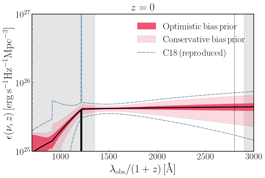
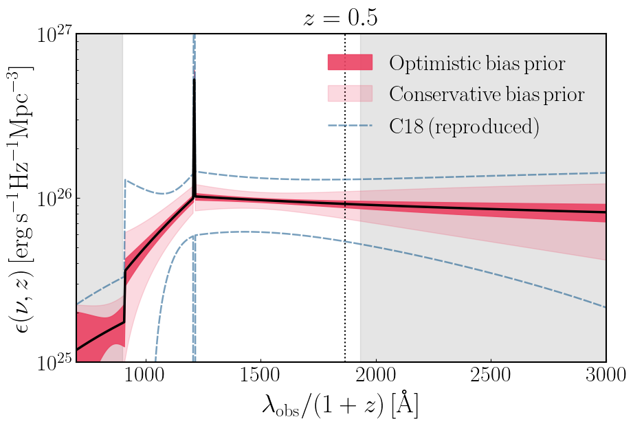
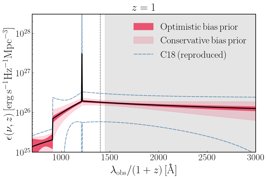
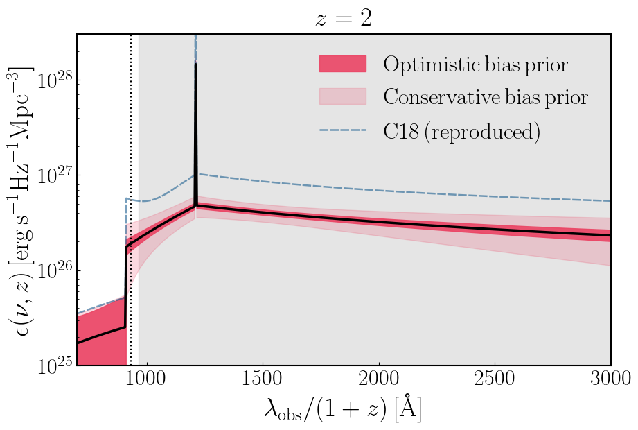
Figure 4: Forecasts at $1\sigma$ on the UV-EBL emissivity $\epsilon(\nu,z)$ at different redshifts for (GALEX$+$ULTRASAT)$\times$DESI, compared with our “post-diction” at $1\sigma$ for GALEX$\times$SDSS as in Ref. Chiang:2018miw (compare with Fig. 6 in their work). We tested both the optimistic and conservative bias priors described in Tab. 4. The gray shaded area delimits the observational window of GALEX$+$ULTRASAT; the gray vertical line shows where GALEX NUV would stop, if ULTRASAT was not included. The parts of the spectrum inside the observed window are directly probed via the CBR, while the others are model-based extrapolations.

IV.3 Forecasts on the volume emissivity

The parameters constrained in the previous section are combined in Eqs. (3), (4), (5) to model the UV-EBL volume emissivity. As discussed in Sec. IV.1, we can assume the local bias $b_{1500}^{z=0}$ is measured, and so convert the $\log_{10}[\epsilon b]_{1500}^{z=0}$ constraints to $\epsilon_{1500}^{z=0}$ and consequently $\epsilon(\nu,z)$, after marginalizing all the other parameters. We analyse results on $\epsilon(\nu,z)$ using this procedure and applying both the conservative and optimistic bias priors in Tab. 4.

Fig. 4 shows our $1\sigma$ forecast constraints on $\epsilon(\nu,z)$ for (GALEX$+$ULTRASAT)$\times$DESI at $z=\{0,0.5,1,2\}$, using the $\vartheta$ parameter set. Here, we also show how the GALEX$\times$SDSS results from the previous section propagate to $\epsilon(\nu,z)$. Our $1\sigma$ forecasts in this case are obtained using the reduced $\vartheta_{\rm C19}$ and including priors from Tab. 4; they can be directly compared with Fig. 6 in C19.

It is evident that (GALEX$+$ULTRASAT)$\times$DESI will provide very good constraints on the UV-EBL volume emissivity reconstruction. Results could be further improved with respect to our findings, if foreground mitigation was taken into account. For example, setting $\mathcal{A}_{\rm fg}\,=\,0$ in Eq. (21) leads to constraints on the emissivity parameters that are $\sim 0.5$ of the ones in Tab. 6. Fig. 4 allows us to further comment on an important aspect of our analysis. Not all the redshifted wavelengths of the UV-EBL emissivity fall in the observational windows of GALEX$+$ULTRASAT. The forecast constraints on $\epsilon(\nu,z)$ that are found in the shaded areas are extrapolated knowing the dependencies of the model parameters in Eqs. (3), (4), (5). The way these have been chosen is agnostic regarding the physics or the type of sources involved: they only require the UV emission to contain a line (Ly$\alpha$), a break (the Lyman break) and a continuum, whose slope varies in the different frequency ranges. In the following section, we discuss the implications this will have in our knowledge of the UV-EBL sources.

IV.4 Forecasts on the UV-EBL sources

The shape of the continuum in the non-ionizing region is showed in C19 to be in good agreement with the model in Ref. Haardt:2011xv , which accounts for galaxy emission and dust extinction. Ref. Haardt:2011xv stresses that the non-ionizing continuum e.g., at 1500$\,{\rm\AA}$, provides valuable information on the star formation rate history (modelled e.g., in Ref. Madau:1995js ) and the metal-enrichment history (e.g., in Refs. Nagamine:2000jb ; Kewley:2007 ), to be tested against the UV luminosity functions (e.g., Wyder:2004ds ; Reddy:2008rj ; Bouwens:2010gp ). Extra-contributions from AGN are negligible in this frequency range, according to Ref. Faucher-Giguere:2019kbp ; on the contrary, the ionizing continuum $\lambda_{\rm rest}<912\,{\rm\AA}$ seems to be AGN-dominated at $z\lesssim 4$. The result, however, depends on the AGN luminosity function (e.g., Hopkins:2006fq ; Kulkarni:2018ebj ; Shen:2020obl ) and on the EBL ionizing photon escape fraction $f_{\rm LyC}$, this being largely uncertain.

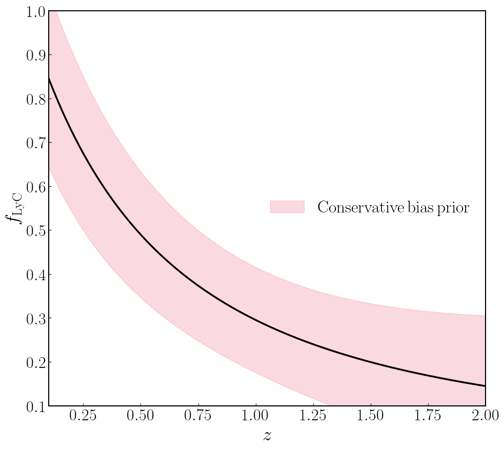
Figure 5: Forecasted $1\sigma$ uncertainties on $f_{\rm LyC}$ using Eq. (8) for (GALEX$+$ULTRASAT)$\times$DESI. Propagated results for GALEX$\times$SDSS are outside of the range of this plot.

Motivated by results in Ref. Alvarez:2012nr , the majority of UV-EBL models Haardt:2011xv ; Alvarez:2012nr ; Robertson:2015uda ; Puchwein:2018arm assume the escape fraction to grow in redshift. C19 manages to provide only upper bounds on $f_{\rm LyC}^{z=1},\,f_{\rm LyC}^{z=2}$; as we show in Fig. 5, instead, (GALEX$+$ULTRASAT)$\times$DESI will be able to constrain these parameters to a level that provides us an overall $1\sigma$ uncertainty on $f_{\rm LyC}$ in Eq. (6) of order 1. These parameters are uncorrelated with bias, hence their constraints do not change when its priors in Tab. 4 are varied.

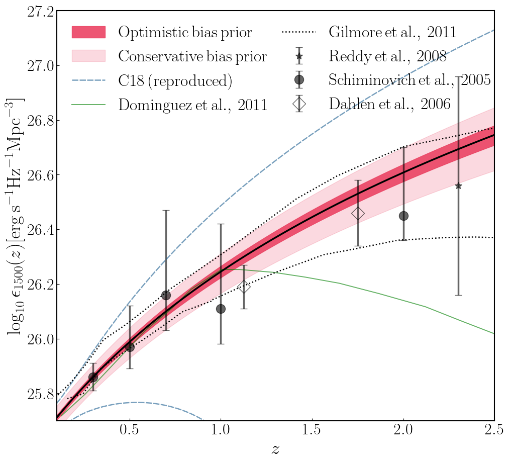
Figure 6: Forecasts at $1\sigma$ on the non-ionizing $\lambda=1500\,{\rm\AA}$ continuum for (GALEX$+$ULTRASAT)$\times$DESI (shaded area), with conservative and optimistic priors on the bias; to get GALEX$\times$SDSS (C19) results, we propagated our “post-diction” in Tab. IV.2. We compare our results with the available data in the literature. Schimonovich et al. data are based on the UV luminosity function of the galaxies in GALEX GALEX-VVDS:2004lih , Dahlen et al. on the one in the GOODS survey from the Hubble Space Telescope Refs. Dahlen:2006sy , while Reddy et al. use a compilation of data from Hubble Reddy:2007bs . The green line reproduces the fitting of Ref. Dominguez:2010bv over multiband data, while the dotted lines are the semi-analytical models obtained in Ref. Gilmore:2011ks with different dust prescriptions.

As a final remark, we refer to Fig. 6 to show that (GALEX$+$ULTRASAT)$\times$DESI will be able to determine the amplitude and redshift evolution of the non-ionizing continuum at $\lambda=1500\,{\rm\AA}$ up to $z\sim 2$, with $1\sigma$ uncertainty $\lesssim 25\%\,(8\%)$ with conservative (optimistic) bias priors, see Tab. 4. We compare our results with the constraints Ref. GALEX-VVDS:2004lih obtained using the galaxy UV luminosity function in GALEX, and the ones Refs. Dahlen:2006sy ; Reddy:2007bs got from data compilations from the Hubble Space Telescope. Moreover, we include the fitting Ref. Dominguez:2010bv realized over multiband Spitzer data, and the semi-analytical models of Ref. Gilmore:2011ks , which account for different dust models.

The improved forecast constrains we obtained on the $\vartheta$ parameters, therefore, can be used to constrain the astrophysical sources of the UV-EBL. With such measurement, the combination of GALEX and ULTRASAT maps will also open the possibility of disentangling any extra-contribution due to emissions beyond galaxies and AGN, e.g., from decaying DM. We will analyse this enticing possibility in an upcoming, dedicated work.

V Conclusion

Many satellites are planned to be launched and start operating over the coming years. Their characteristics and goals are the most diverse, and it is crucial to understand how to exploit their data as best as we can. New observables and estimators will be needed, in order to probe the Universe at various redshifts and scales, so as to deepen our understanding of cosmic evolution.

Among these space-borne observatories, the Ultraviolet Transient Astronomy Satellite (ULTRASAT, Sagiv:2013rma ; ULTRASAT:2022 ; Shvartzvald:2023ofi ) will observe the near-UV (NUV) range between $2300\,\rm\AA$ and $2900\,\rm\AA$: its main goal will be the study of transients, e.g., supernovae, variable stars, AGN and electromagnetic counterparts to gravitational-wave sources. To perform its intended analysis, ULTRASAT will first of all build a reference full sky map, which itself will contain an enormous amount of information.

Besides the emission from resolved galaxies, such map will collect diffuse light of astrophysical and cosmological origin, produced e.g., by unresolved galaxies, AGN, dust Madau:2014bja ; Bernstein:2001sq ; Haardt:2011xv or more exotic components such as decaying or annihilating dark matter, or direct-collapse black holes Dwek:1998bk ; Bond:1985pc ; Yue:2012dd ; Creque-Sarbinowski:2018ebl ; Bernal:2020lkd . The overlap of all these processes produce the extragalactic background light (EBL), which in the UV regime is not yet well constrained.

The ULTRASAT full-sky map will be a good tool to boost our knowledge in this field; to find different ways to exploit its potential, a possible way is to look at the studies that were performed on the full-sky map realized with the All Sky and Medium Imaging Surveys performed by the Galaxy Evolution Explorer (GALEX, Martin:2004yr ; Morrissey:2007hv ). ULTRASAT, similarly to GALEX, will observe a broad frequency range, therefore it will collect the integrated UV emission produced over a wide redshift range, and map its intensity fluctuations as function of sky position.

The GALEX diffuse light map has been analysed by the authors of Ref. Chiang:2018miw ( C19) via the clustering-based redshift technique (CBR, Newman:2008mb ; McQuinn:2013ib ; Menard:2013aaa ): by cross correlating it with the spectroscopic galaxy catalogs from the Sloan Digital Sky Survey (SDSS, SDSS:2004dnq ; Reid:2015gra ), they reconstructed the redshift evolution of the comoving volume emissivity of the UV-EBL, providing constraints on the parameters that describe the non-ionizing continuum and the Ly$\alpha$ line. These, in turn, can be used to constrain properties such as the star formation rate or metallicity history.

A very interesting aspect of CBR is that it is only sensitive to extragalactic contributions; the presence of foregrounds does not alter its signal, while it contributes to the overall noise budget. A similar study was performed in Ref. Scott:2021zue ( S21) to forecast the constraining power of the Cosmological Advanced Survey Telescope for Optical and UV Research (CASTOR, Cote:2019 ).

In this work, we studied how to build forecasts for the CBR technique when this is applied to the cross correlation between a broadband UV survey and a spectroscopic galaxy catalog. We summarized how to model the main observable that is required in this context, namely the angular cross correlation between intensity measurements in pixels and galaxies, and we derived an analytical expression to estimate its noise. We then ran a Fisher forecast with respect to the parameters that model the UV-EBL comoving volume emissivity.

To validate our method, we first of all reproduced the setup of the analysis performed in  C19, where GALEX$\times$SDSS is considered: the constraints we obtained are in the same ballpark of the actual results. Once we tested the reliability of our analysis, we applied it to forecast the cross correlation between ULTRASAT full-sky map and galaxies in the spectroscopic bins of the Dark Energy Spectroscopic Instrument (DESI, DESI:2013agm ; DESI:2016fyo ; DESI:2016igz ). We verified that the smaller redshift uncertainty and larger galaxy number density DESI has with respect to SDSS, together with the smaller noise variance and larger field of view in the ULTRASAT map, will imply an improvement in the ULTRASAT$\times$DESI constraints with respect to GALEX$\times$SDSS, when applied to the same parameter set and under the same conditions.

Driven by this result, we applied the forecasted CBR analysis also to the (GALEX$+$ULTRASAT)$\times$DESI full setup. We showed that the large redshift range and the improved sensitivity will allow us to constrain with good accuracy all the parameters in the emissivity model. Once propagated to the emissivity uncertainty, these will lead to the forecasts shown in Fig. 4, where we accounted for different choices of priors on the bias parameters.

We found that (GALEX$+$ULTRASAT)$\times$DESI will be able to constrain the full UV emissivity frequency dependence in the redshift range $z\lesssim 2$. In our work, we assumed that this is composed by different contributions: the non-ionizing continuum, the Ly$\alpha$ line and the ionizing continuum above the Lyman break. The amplitude and slope of each of these elements is determined by the UV-EBL sources; therefore, this measurement will provide interesting insights on the astrophysics. In particular, in Fig. 5, we show the constraining power we obtained on the ionizing photon escape fraction, for which C19 only managed to provide upper bounds. In Fig. 6, instead, we showed our forecasts on the non-ionizing EBL emissivity at $\lambda=1500\,{\rm\AA}$. Here, current data show an overall agreement with the EBL models that accounts for galaxies, AGN emissions and dust. The improvement (GALEX$+$ULTRASAT)$\times$DESI will bring will foster our understanding of this regime, opening the window to the detection of exotic cosmological emissions, if any.

To conclude, we stress once again how the study of the UV extragalactic background light will be crucial in the upcoming years. ULTRASAT, with its reference map, will offer the possibility of mapping its intensity fluctuations across the full sky, offering a tool to probe the underlying large scale structure in a novel, alternative way. To be able to exploit the enormous amount of scientific information it will contain, it is important to develop specific tools for its analysis; the cross correlation with galaxy surveys, in particular in the context of the clustering-based redshift analysis, is indeed one of them.

- (1) A. Cooray, “Extragalactic Background Light: Measurements and Applications,” [arXiv:1602.03512 [astro-ph.CO]].
- (2) T. P. Sasseen, M. Lampton, S. Bowyer, and X. Wu, “Observations of the Galactic and Extragalactic Background with the Far-Ultraviolet Space Telescope (FAUST) ,” Astrophysical Journal 447, 630 (1995)
- (3) J. Murthy, J. Doyle, E. Matthew, R. C. Henry and J. B. Holberg, J. B. “An Analysis of 17 Years of Voyager Observations of the Diffuse Far-Ultraviolet Radiation Field,” Astrophys. J, 522, 904-914 (1999)
- (4) J. Edelstein, S. Bowyer and M. Lampton 2000, “Reanalysis of Voyager Ultraviolet Spectrometer Limits to the Extreme-Ultraviolet and Far-Ultraviolet Diffuse Astronomical Flux,” Astrophys. J. 539, 187-190 (2000)
- (5) T. M. Brown, R. A. Kimble, H. C. Ferguson, J. P. Gardner, N. R. Collins and R. S. Hill, “Measurements of the diffuse ultraviolet background and the terrestrial airglow with the space telescope imaging spectrograph,” Astron. J. 120, 1153 (2000) [arXiv:astro-ph/0004147 [astro-ph]].
- (6) R. A. Bernstein, W. L. Freedman and B. F. Madore, “The First detections of the extragalactic background light at 3000, 5500, and 8000A. 3. Cosmological implications,” Astrophys. J. 571, 107 (2002) [arXiv:astro-ph/0112170 [astro-ph]].
- (7) J. Murthy, R. C. Henry and N. V. Sujatha, “Mapping the Diffuse Ultraviolet Sky with GALEX,” Astrophys. J. 724, 1389-1395 (2010) [arXiv:1009.4530 [astro-ph.GA]].
- (8) R. Hill, K. W. Masui and D. Scott, “The Spectrum of the Universe,” Appl. Spectrosc. 72, no.5, 663-688 (2018) [arXiv:1802.03694 [astro-ph.CO]].
- (9) P. Madau and M. Dickinson, “Cosmic Star Formation History,” Ann. Rev. Astron. Astrophys. 52, 415-486 (2014) [arXiv:1403.0007 [astro-ph.CO]].
- (10) D. Schiminovich, P. Friedman, C. Martin and P. Morrissey, “The narrow-band ultraviolet imaging experiment for wide-field surveys (nuviews)-i: dust scattered continuum,” Astrophys. J. Lett. 563, L161-L164 (2001) [arXiv:astro-ph/9905362 [astro-ph]].
- (11) E. Dwek, R. G. Arendt, M. G. Hauser, D. Fixsen, T. Kelsall, D. Leisawitz, Y. C. Pei, E. L. Wright, J. C. Mather and S. H. Moseley, et al. “The COBE diffuse infrared background experiment search for the cosmic infrared background. 4. Cosmological implications,” Astrophys. J. 508, 106 (1998) [arXiv:astro-ph/9806129 [astro-ph]].
- (12) J. R. Bond, B. J. Carr and C. J. Hogan, “Spectrum and Anisotropy of the Cosmic Infrared Background,” Astrophys. J. 306, 428-450 (1986)
- (13) B. Yue, A. Ferrara, R. Salvaterra and X. Chen, “The Contribution of High Redshift Galaxies to the Near-Infrared Background,” Mon. Not. Roy. Astron. Soc. 431, 383 (2013) [arXiv:1208.6234 [astro-ph.CO]].
- (14) R. C. Henry, J. Murthy, J. Overduin and J. Tyler, Astrophys. J. 798, 14 (2015) doi:10.1088/0004-637X/798/1/14 [arXiv:1404.5714 [astro-ph.GA]].
- (15) C. Creque-Sarbinowski and M. Kamionkowski, “Searching for Decaying and Annihilating Dark Matter with Line Intensity Mapping,” Phys. Rev. D 98, no.6, 063524 (2018) [arXiv:1806.11119 [astro-ph.CO]].
- (16) J. L. Bernal, A. Caputo and M. Kamionkowski, “Strategies to Detect Dark-Matter Decays with Line-Intensity Mapping,” Phys. Rev. D 103, no.6, 063523 (2021) [erratum: Phys. Rev. D 105, no.8, 089901 (2022)] [arXiv:2012.00771 [astro-ph.CO]].
- (17) I. Sagiv, A. Gal-Yam, E. O. Ofek, E. Waxman, O. Aharonson, E. Nakar, D. Maoz, B. Trakhtenbrot, S. R. Kulkarni and E. S. Phinney, et al. “Science with a wide-field UV transient explorer,” Astron. J. 147, 79 (2014) [arXiv:1303.6194 [astro-ph.CO]].
- (18) S. Ben-Ami, Y. Shvartzvald, E. Waxman, U. Netzer, Y. Yaniv, V. M. Algranatti, A. Gal-Yam, O. Lapid, E. Ofek, J. Topaz and I. Arcavi, et al. “The scientific payload of the Ultraviolet Transient Astronomy Satellite (ULTRASAT) [arXiv:2208.00159]
- (19) Y. Shvartzvald, E. Waxman, A. Gal-Yam, E. O. Ofek, S. Ben-Ami, D. Berge, M. Kowalski, R. Bühler, S. Worm and J. E. Rhoads, et al. “ULTRASAT: A wide-field time-domain UV space telescope,” [arXiv:2304.14482 [astro-ph.IM]].
- (20) D. C. Martin, J. Fanson, D. Schiminovich, P. Morrissey, P. G. Friedman, T. A. Barlow, T. Conrow, R. Grange, P. N. Jelinsky and B. Milliard, et al. “The Galaxy Evolution Explorer: A Space ultraviolet survey mission,” Astrophys. J. Lett. 619, L1-L6 (2005) [arXiv:astro-ph/0411302 [astro-ph]].
- (21) P. Morrissey, T. Conrow, T. A. Barlow, T. Small, M. Seibert, T. K. Wyder, T. Budavari, S. Arnouts, P. G. Friedman and K. Forster, et al. “The Calibration and Data Products of the Galaxy Evolution Explorer,” [arXiv:0706.0755 [astro-ph]].
- (22) J. Murthy, “GALEX diffuse observations of the sky: the data,” The Astrophysical Journal, 213, 32 (2014)
- (23) N. V. Sujatha, J. Murthy, R. Suresh, R. C. Henry and L. Bianchi, “GALEX Observations of Diffuse Ultraviolet Emission from Draco,” Astrophys. J. 723, 1549-1557 (2010) [arXiv:1009.3348 [astro-ph.GA]].
- (24) N. V. Sujatha, J. Murthy, A. Karnataki, R. C. Henry and L. Bianchi, “GALEX Observations of Diffuse UV Radiation at High Spatial Resolution from the Sandage Nebulosity,” Astrophys. J. 692, 1333-1338 (2009) [arXiv:0807.0189].
- (25) E. T. Hamden, D. Schiminovich, M Seibert, “The Diffuse Galactic Far-ultraviolet Sky,” Astrophys. J. 779, 2, (2013) [arXiv:1311.0875].
- (26) J. Murthy, “The diffuse ultraviolet foreground,” Astrophysics and Space Science, 349, 1, (2013) [arXiv:1307.5232].
- (27) M. S. Akshaya, J. Murthy, S. Ravichandran, R. C. Henry, J. Overduin, “The Diffuse Radiation Field at High Galactic Latitudes,” Astrophys. J. 858, 2, 1538-4375 (2018) [arXiv:1701.07644].
- (28) J. Murthy, “Modelling dust scattering in our Galaxy”, Monthly Notices of the Royal Astronomical Society, 459, 2, (2016) [arXiv:10.1093/mnras/stw755]
- (29) Yi-Kuan Chiang and Brice Ménard, “Extragalactic Imprints in Galactic Dust Maps” The Astrophysical Journal 870, 2, 120 (2019) [arXiv:1808.03294]
- (30) G. Saikia and P. Shalima and R. Gogoi and A. Pathak, “Probing the infrared counterparts of diffuse far-ultraviolet sources in the Galaxy” Planetary Space Science 149 (2017) [arXiv:1705.00380]
- (31) B. Welch and S. McCandliss, and D. Coe, “Galaxy Cluster Contribution to the Diffuse Extragalactic Ultraviolet Background” The Astrophysical Journal 159, 6, 269 (2020) [arXiv:2004.09401]
- (32) Y. K. Chiang, B. Ménard and D. Schiminovich, “Broadband Intensity Tomography: Spectral Tagging of the Cosmic UV Background,” Astrophys. J. 877, no.2, 150 (2019) [arXiv:1810.00885 [astro-ph.CO]].
- (33) J. A. Newman, “Calibrating Redshift Distributions Beyond Spectroscopic Limits with Cross-Correlations,” Astrophys. J. 684, 88 (2008) [arXiv:0805.1409 [astro-ph]].
- (34) M. McQuinn and M. White, “On using angular cross-correlations to determine source redshift distributions,” Mon. Not. Roy. Astron. Soc. 433, 2857-2883 (2013) [arXiv:1302.0857 [astro-ph.CO]].
- (35) B. Ménard, R. Scranton, S. Schmidt, C. Morrison, D. Jeong, T. Budavari and M. Rahman, “Clustering-based redshift estimation: method and application to data,” [arXiv:1303.4722 [astro-ph.CO]].
- (36) M. Rahman, B. Ménard, R. Scranton, S. J. Schmidt and C. B. Morrison, “Clustering-based Redshift Estimation: Comparison to Spectroscopic Redshifts,” Mon. Not. Roy. Astron. Soc. 447, 3500 (2015) [arXiv:1407.7860 [astro-ph.GA]].
- (37) V. Scottez, Y. Mellier, B. R. Granett, T. Moutard, M. Kilbinger, M. Scodeggio, B. Garilli, M. Bolzonella, S. de la Torre and L. Guzzo, et al. “Clustering-based redshift estimation: application to VIPERS/CFHTLS,” Mon. Not. Roy. Astron. Soc. 462, no.2, 1683-1696 (2016) [arXiv:1605.05501 [astro-ph.CO]].
- (38) C. B. Morrison, H. Hildebrandt, S. J. Schmidt, I. K. Baldry, M. Bilicki, A. Choi, T. Erben and P. Schneider, “The-wiZZ: Clustering redshift estimation for everyone,” Mon. Not. Roy. Astron. Soc. 467, no.3, 3576-3589 (2017) [arXiv:1609.09085 [astro-ph.CO]].
- (39) C. Davis et al. [DES], “Cross-Correlation Redshift Calibration without Spectroscopic Calibration Samples in DES Science Verification Data,” Mon. Not. Roy. Astron. Soc. 477, no.2, 2196-2208 (2018) [arXiv:1707.08256 [astro-ph.CO]].
- (40) S. J. Schmidt, B. Ménard, R. Scranton, C. B. Morrison, M. Rahman and A. M. Hopkins, “Inferring the Redshift Distribution of the Cosmic Infrared Background,” Mon. Not. Roy. Astron. Soc. 446, 2696-2708 (2015) [arXiv:1407.0031 [astro-ph.CO]].
- (41) E. D. Kovetz, A. Raccanelli and M. Rahman, “Cosmological Constraints with Clustering-Based Redshifts,” Mon. Not. Roy. Astron. Soc. 468, no.3, 3650-3656 (2017) [arXiv:1606.07434 [astro-ph.CO]].
- (42) G. Scelfo, M. Spinelli, A. Raccanelli, L. Boco, A. Lapi and M. Viel, “Gravitational waves × HI intensity mapping: cosmological and astrophysical applications,” JCAP 01, no.01, 004 (2022) [arXiv:2106.09786 [astro-ph.CO]].
- (43) M. R. Blanton et al. [SDSS], “NYU-VAGC: A Galaxy catalog based on new public surveys,” Astron. J. 129, 2562-2578 (2005) [arXiv:astro-ph/0410166 [astro-ph]].
- (44) B. Reid, S. Ho, N. Padmanabhan, W. J. Percival, J. Tinker, R. Tojeiro, M. White, D. J. Eisenstein, C. Maraston and A. J. Ross, et al. “SDSS-III Baryon Oscillation Spectroscopic Survey Data Release 12: galaxy target selection and large scale structure catalogues,” Mon. Not. Roy. Astron. Soc. 455, no.2, 1553-1573 (2016) [arXiv:1509.06529 [astro-ph.CO]].
- (45) B. R. Scott, P. U. Sanderbeck and S. Bird, “Forecasts for broad-band intensity mapping of the ultraviolet-optical background with CASTOR and SPHEREx,” Mon. Not. Roy. Astron. Soc. 511, no.4, 5158-5170 (2022) [arXiv:2104.00017 [astro-ph.CO]].
- (46) P. Cote, B. Abraham and M. Balog et al., “CASTOR: A Flagship Canadian Space Telescope,” Zenodo, in Canadian Long Range Plan for Astronomy and Astrophysics White Papers (2019)
- (47) O. Doré et al. [SPHEREx], “Cosmology with the SPHEREX All-Sky Spectral Survey,” [arXiv:1412.4872 [astro-ph.CO]].
- (48) O. Doré et al. [SPHEREx], “Science Impacts of the SPHEREx All-Sky Optical to Near-Infrared Spectral Survey: Report of a Community Workshop Examining Extragalactic, Galactic, Stellar and Planetary Science,” [arXiv:1606.07039 [astro-ph.CO]].
- (49) O. Doré et al. [SPHEREx], “Science Impacts of the SPHEREx All-Sky Optical to Near-Infrared Spectral Survey II: Report of a Community Workshop on the Scientific Synergies Between the SPHEREx Survey and Other Astronomy Observatories,” [arXiv:1805.05489 [astro-ph.IM]].
- (50) M. Levi et al. [DESI], “The DESI Experiment, a whitepaper for Snowmass 2013,” [arXiv:1308.0847 [astro-ph.CO]].
- (51) A. Aghamousa et al. [DESI], “The DESI Experiment Part I: Science,Targeting, and Survey Design,” [arXiv:1611.00036 [astro-ph.IM]].
- (52) A. Aghamousa et al. [DESI], “The DESI Experiment Part II: Instrument Design,” [arXiv:1611.00037 [astro-ph.IM]].
- (53) E. D. Kovetz, M. P. Viero, A. Lidz, L. Newburgh, M. Rahman, E. Switzer, M. Kamionkowski, J. Aguirre, M. Alvarez and J. Bock, et al. “Line-Intensity Mapping: 2017 Status Report,” [arXiv:1709.09066 [astro-ph.CO]].
- (54) J. L. Bernal and E. D. Kovetz, “Line-intensity mapping: theory review with a focus on star-formation lines,” Astron. Astrophys. Rev. 30, no.1, 5 (2022) [arXiv:2206.15377 [astro-ph.CO]].
- (55) Bastian-Querner B., Kaipachery N. et al., “Sensor characterization for the ULTRASAT space telescope”, UV/Optical/IR Space Telescopes and Instruments: Innovative Technologies and Concepts X (SPIE), 2021, [arXiv:/2108.02521]
- (56) A. Asif, M. Barschke, B. Bastian-Querner, D. Berge, R. Bühler, N. De Simone, G. Giavitto, J. M. H. Crespo, N. Kaipachery and M. Kowalski, et al. doi:10.1117/12.2594253 [arXiv:2108.01493 [astro-ph.IM]].
- (57) G. Adame et al. [DESI], “Validation of the Scientific Program for the Dark Energy Spectroscopic Instrument,” [arXiv:2306.06307 [astro-ph.CO]].
- (58) F. Haardt and P. Madau, “Radiative transfer in a clumpy universe: IV. New synthesis models of the cosmic UV/X-ray background,” Astrophys. J. 746, 125 (2012) [arXiv:1105.2039 [astro-ph.CO]].
- (59) P. Madau, “Radiative transfer in a clumpy universe: The Colors of high-redshift galaxies,” Astrophys. J. 441, 18 (1995) doi:10.1086/175332
- (60) D. Schiminovich et al. [GALEX-VVDS], “The GALEX-VVDS measurement of the evolution of the far-ultraviolet luminosity density and the cosmic star formation rate,” Astrophys. J. Lett. 619, L47 (2005) [arXiv:astro-ph/0411424 [astro-ph]].
- (61) A. Alavi and B. Siana and J. Richard, et al., “THE EVOLUTION OF THE FAINT END OF THE UV LUMINOSITY FUNCTION DURING THE PEAK EPOCH OF STAR FORMATION (1¡ z¡ 3),” Astrophys. Journal 832, 56 (2016)
- (62) J. E. Gunn and B. A. Peterson, “On the Density of Neutral Hydrogen in Intergalactic Space,” The Astrophys. Journal 142, 11 (1965)
- (63) C. C. Steidel, W. L. W. Sargent, “The Effect of the Lyman-Alpha Forest on the Ultraviolet Continua of Very High Redshift Quasars,” The Astrophys. Journal 313 2, 171 (1987)
- (64) A. K. Inoue, I. Shimizu and I. Iwata, “An updated analytic model for the attenuation by the intergalactic medium,” Mon. Not. Roy. Astron. Soc. 442, no.2, 1805-1820 (2014) [arXiv:1402.0677 [astro-ph.CO]].
- (65) N. Y. Gnedin and J. P. Ostriker, “Reionization of the universe and the early production of metals,” Astrophys. J. 486, 581 (1997) [arXiv:astro-ph/9612127 [astro-ph]].
- (66) A. H. Maller, D. H. McIntosh, N. Katz and M. D. Weinberg, “The Galaxy angular correlation functions and power spectrum from the Two Micron All Sky Survey,” Astrophys. J. 619, 147-160 (2005) [arXiv:astro-ph/0304005 [astro-ph]].
- (67) M. S. Vogeley, A. Szalay, “Eigenmode Analysis of Galaxy Redshift Surveys. I. Theory and Methods,” Astrophys. J. 465, 34 (1996) [arXiv:astro-ph/9601185 [astro-ph]].
- (68) M. Tegmark, A. Taylor and A. Heavens, “Karhunen-Loeve eigenvalue problems in cosmology: How should we tackle large data sets?,” Astrophys. J. 480, 22 (1997) [arXiv:astro-ph/9603021 [astro-ph]].
- (69) I. Zehavi et al. [SDSS], “Galaxy Clustering in the Completed SDSS Redshift Survey: The Dependence on Color and Luminosity,” Astrophys. J. 736, 59-88 (2011) [arXiv:1005.2413 [astro-ph.CO]].
- (70) K. Nagamine, M. Fukugita, R. Cen and J. P. Ostriker, “Star formation history and stellar metallicity distribution in a cold dark matter Universe,” Astrophys. J. 558, 497 (2001) [arXiv:astro-ph/0011472 [astro-ph]].
- (71) L. Kewley and H. A. Kobulnicky, “THE METALLICITY HISTORY OF DISK GALAXIES,” in Island Universes, 435-440 (2007)
- (72) N. A. Reddy and C. C. Steidel, “A Steep Faint-End Slope of the UV Luminosity Function at z~2-3: Implications for the Global Stellar Mass Density and Star Formation in Low Mass Halos,” Astrophys. J. 692, 778-803 (2009) [arXiv:0810.2788 [astro-ph]].
- (73) R. J. Bouwens, G. D. Illingworth, P. A. Oesch, I. Labbe, M. Trenti, P. van Dokkum, M. Franx, M. Stiavelli, C. M. Carollo and D. Magee, et al. “UV Luminosity Functions from 113 z~7 and z~8 Lyman-Break Galaxies in the ultra-deep HUDF09 and wide-area ERS WFC3/IR Observations,” Astrophys. J. 737, 90 (2011) [arXiv:1006.4360 [astro-ph.CO]].
- (74) C. A. Faucher-Giguère, “A cosmic UV/X-ray background model update,” Mon. Not. Roy. Astron. Soc. 493, no.2, 1614-1632 (2020) [arXiv:1903.08657 [astro-ph.CO]].
- (75) P. F. Hopkins, G. T. Richards and L. Hernquist, “An Observational Determination of the Bolometric Quasar Luminosity Function,” Astrophys. J. 654, 731-753 (2007) [arXiv:astro-ph/0605678 [astro-ph]].
- (76) G. Kulkarni, G. Worseck and J. F. Hennawi, “Evolution of the AGN UV luminosity function from redshift 7.5,” Mon. Not. Roy. Astron. Soc. 488, no.1, 1035-1065 (2019) [arXiv:1807.09774 [astro-ph.GA]].
- (77) X. Shen, P. F. Hopkins, C. A. Faucher-Giguère, D. M. Alexander, G. T. Richards, N. P. Ross and R. C. Hickox, “The bolometric quasar luminosity function at z = 0–7,” Mon. Not. Roy. Astron. Soc. 495, no.3, 3252-3275 (2020) [arXiv:2001.02696 [astro-ph.GA]].
- (78) M. A. Alvarez, K. Finlator and M. Trenti, “Constraints on the Ionizing Efficiency of the First Galaxies,” Astrophys. J. Lett. 759, L38 (2012) [arXiv:1209.1387 [astro-ph.CO]].
- (79) B. E. Robertson, R. S. Ellis, S. R. Furlanetto and J. S. Dunlop, “Cosmic Reionization and Early Star-forming Galaxies: a Joint Analysis of new Constraints From Planck and the Hubble Space Telescope,” Astrophys. J. Lett. 802, no.2, L19 (2015) [arXiv:1502.02024 [astro-ph.CO]].
- (80) E. Puchwein, F. Haardt, M. G. Haehnelt and P. Madau, “Consistent modelling of the meta-galactic UV background and the thermal/ionization history of the intergalactic medium,” Mon. Not. Roy. Astron. Soc. 485, no.1, 47-68 (2019) [arXiv:1801.04931 [astro-ph.GA]].
- (81) T. K. Wyder, M. A. Treyer, B. Milliard, D. Schiminovich, S. Arnouts, T. Budavari, T. A. Barlow, L. Bianchi, Y. I. Byun and J. Donas, et al. “The UV galaxy luminosity function in the Local Universe from GALEX data,” Astrophys. J. Lett. 619, L15-L18 (2005) [arXiv:astro-ph/0411364 [astro-ph]].
- (82) T. Dahlen, B. Mobasher, M. Dickinson, H. C. Ferguson, M. Giavalisco, C. Kretchmer and S. Ravindranath, “Evolution of the Luminosity Function, Star Formation Rate, Morphology and Size of Star-forming Galaxies Selected at Rest-frame 1500A and 2800A,” Astrophys. J. 654, 172-185 (2006) [arXiv:astro-ph/0609016 [astro-ph]].
- (83) N. A. Reddy, C. C. Steidel, M. Pettini, K. L. Adelberger, A. E. Shapley, D. K. Erb and M. Dickinson, “Multi-Wavelength Constraints on the Cosmic Star Formation History from Spectroscopy: The Rest-Frame UV, H-alpha, and Infrared Luminosity Functions at Redshifts 1.9~z~3.4,” Astrophys. J. Suppl. 175, 48 (2008) [arXiv:0706.4091 [astro-ph]].
- (84) A. Dominguez, J. R. Primack, D. J. Rosario, F. Prada, R. C. Gilmore, S. M. Faber, D. C. Koo, R. S. Somerville, M. A. Perez-Torres and P. Perez-Gonzalez, et al. “Extragalactic Background Light Inferred from AEGIS Galaxy SED-type Fractions,” Mon. Not. Roy. Astron. Soc. 410, 2556 (2011) [arXiv:1007.1459 [astro-ph.CO]].
- (85) R. C. Gilmore, et al., “Semi-analytic modeling of the EBL and consequences for extragalactic gamma-ray spectra,” Mon. Not. Roy. Astron. Soc. 422, 3189 (2012) [arXiv:1104.0671 [astro-ph.CO]].