Relevance of one-loop SMEFT matching in the 2HDM

[12mm]12mm The Two-Higgs Doublet Model (2HDM) is a well understood alternative to the Standard Model of particle physics. If the new particles included in the 2HDM are at an energy scale much greater than the weak scale, the theory can be matched to the Standard Model Effective Field Theory (SMEFT). We compute for the first time the complete one-loop matching at dimension-6. We compare its numerical impact with that of tree-level matching at dimension-8 by performing a global fit to single Higgs and precision electroweak measurements, and we emphasize the importance of comparing one-loop SMEFT results with corresponding one-loop results in the full 2HDM model. In the SMEFT, we consider the relative importance of both one-loop matching and the inclusion of renormalization group evolution. Our results demonstrate the necessity of studying the impact of various expansions to quantify the uncertainties of the SMEFT matching.

1 Introduction

Since the observation at the LHC of a light Higgs boson with properties approximately those predicted by the Standard Model (SM), much of the focus has turned to searches for new physics at higher energy scales. These studies follow a two pronged approach: one either searches directly for heavy new particles that are typically predicted in extensions of the SM, or uses an effective field theory (EFT) framework to look for weak scale manifestations of the new physics. Here we follow the second alternative, resorting to the Standard Model Effective Field Theory (SMEFT) (for reviews, see Refs. [1, 2]). The SMEFT contains an infinite tower of higher-dimensional $\textrm{SU}(3)_{c}\times\textrm{SU}(2)_{L}\times\textrm{U}(1)_{Y}$ invariant operators,

$$\mathcal{L}_{\rm{SMEFT}}=\mathcal{L}_{\rm{SM}}+\sum_{i}\frac{C_{i}O_{i}}{\Lambda^{2}}+\sum_{j}\frac{C_{j}O_{j}}{\Lambda^{4}}+...\,\,,$$ (1)

where $\mathcal{L}_{\rm{SM}}$ is the renormalizable SM Lagrangian, $\Lambda$ is the scale of some conjectured ultraviolet (UV) complete model and the $C_{i}$ are usually known as Wilson coefficients (WCs). In any given model of UV physics, the WCs can be calculated in terms of the model parameters.

The goal of the SMEFT program is to experimentally observe a pattern of non-zero WCs, and thus infer features of the physics at the high scale. It is then of paramount importance to investigate how well the WCs can replicate the UV physics at low energy scales. A usual strategy is to flip the problem upside down, by starting from a particular UV model, and by performing the matching between that model and the SMEFT [3, 4, 5, 6, 7, 8]. Although a tree-level matching with dimension-6 operators is the obvious first step, it is clear that there are scenarios where this is insufficient [9, 10, 11, 12, 13, 14, 15]. Improvements have been made either in the direction of increasing the dimension [16, 17, 18, 19], or in the direction of one-loop matching [5, 6, 20, 21, 22]. The complexity of the matching procedure and interpretation of data increases with each of these improvements. A relevant question is then: which of these directions is necessary to quickly approach the UV model using the SMEFT approach?

We address this question by considering the Two-Higgs Doublet Model (2HDM) [23] with a softly broken $Z_{2}$ symmetry. This model is an excellent test case, since the tree-level matching to the SMEFT up to dimension-8 is known [17], and the phenomenological consequences of the full 2HDM model are well studied [24, 25]. The matching procedure of a UV model like the 2HDM to the SMEFT mainly follows two approaches: diagrammatic and functional methods. The diagrammatic approach involves the computation of amplitudes in the UV and in the EFT, and solving for WCs in terms of the new physics couplings. The functional methods proceed with the computation of effective action formulae, defined by the covariant derivatives and the new physics interactions. Both methods involve lengthy and cumbersome mathematics, where automatization can help immensely. Currently, there are four packages that facilitate automated SMEFT matching: MatchingTools [29], CoDEx [30], Matchmakereft [31] and Matchete [32].

In this work, we perform the complete one-loop matching of the 2HDM to the SMEFT with dimension-6 operators, using the packages Matchmakereft and Matchete. We create an implementation of the 2HDM for these software packages, and check that their results agree. The results of these two codes have been checked to agree in many other scenarios, including Higgs singlet model [6], vector-like lepton extension of the SM [32], Type-III seesaw model [22] and a lepto-quark model [33]. We also use Matchete to calculate the tree-level dimension-8 WCs, by exploiting the capacity of this software to create and solve SuperTraces [34] at arbitrary mass-dimension, without additional inputs from the users. The WCs which are generated at tree-level (both dimension-6 and dimension-8) and which are relevant for this study fully agree with those of Ref. [17].

Here, we are interested in using the 2HDM to test the quality of SMEFT matchings. Specifially, we compare the numerical importance of one-loop matching with dimension-6 operators, on the one hand, and tree-level matching with dimension-8 operators, on the other. This we do by examining both precision electroweak and single Higgs measurements. It is of particular importance to compare the SMEFT one-loop matched results to predictions for observables in the full 2HDM that are also computed to one-loop [35, 36]. A similar study performed for a Higgs singlet model found that the effects of the one-loop dimension-6 matching in that case were small [37].

The paper is organized as follows. In Section 2, we briefly summarize the 2HDM in order to set notation, and we discuss the constraints on the parameters of the model. Section 3 is devoted to the matching between the 2HDM and the SMEFT; we discuss how decoupling can be used to perform a consistent expansion, and present details of both the tree-level matching up to dimension-8 operators and the one-loop matching. We present our numerical results in Section 4, discussing fits for electroweak precision observables (EWPOs) first, and to Higgs signal strengths afterwards. We compare numerical results obtained using various SMEFT and loop expansions. Section 5 contains some conclusions along with a discussion of future directions for study. Some appendices complement the main text: Appendix A contains formulae in the 2HDM, Appendix B contains the one-loop matching results relevant for our analyses, and Appendix C provides details on the fits. Details of our 2HDM implementation of Matchmakereft and Matchete can be found in the auxiliary material [38].

2 2HDM

2.1 The model

For this review of the 2HDM, we follow Ref. [17] closely (for more details, cf. Refs. [25, 39, 24]). The model contains a second scalar doublet $\Phi_{2}$ along with the SM scalar doublet $\Phi_{1}$, with real vacuum expectation values (vevs) $v_{2}/\sqrt{2}$ and $v_{1}/\sqrt{2}$, respectively. A softly broken $Z_{2}$ symmetry is imposed on the potential, under which the scalar doublets transform as $\Phi_{1}\to\Phi_{1}$ and $\Phi_{2}\to-\Phi_{2}$. It is convenient to rotate the fields to the Higgs basis, with doublets $H_{1}$ and $H_{2}$:

$$\left(\begin{array}[]{c}H_{1}\\ H_{2}\end{array}\right)=\left(\begin{array}[]{cc}c_{\beta}&s_{\beta}\\ -s_{\beta}&c_{\beta}\end{array}\right)\left(\begin{array}[]{c}\Phi_{1}\\ \Phi_{2}\end{array}\right),$$ (8)

where we introduced the short notation $s_{x}\equiv\sin x,c_{x}\equiv\cos x$, and $\tan\beta=v_{2}/v_{1}$. This implies that, in the Higgs basis, only $H_{1}$ has a vev, $v/\sqrt{2}$, with $v=\sqrt{v_{1}^{2}+v_{2}^{2}}=246$ GeV.

We focus on two terms of the Lagrangian, $\mathcal{L}_{2\mathrm{HDM}}\supset\mathcal{L}_{Y}-V$ (representing the Yukawa terms and the potential, respectively), and we write them both in the Higgs basis. The $Z_{2}$ symmetry is extended to the fermions in order to avoid flavor changing neutral currents at tree-level. There are four possibilities for such an extension, leading to four types of 2HDM: Type-I, Type-II, Type-L and Type-F. We write $\mathcal{L}_{Y}$ as:

$$\mathcal{L}_{Y}=-Y_{u}{\overline{q}}_{L}{\tilde{H}}_{1}u_{R}-Y_{d}{\overline{q}}_{L}H_{1}d_{R}-Y_{e}{\overline{l}}_{L}H_{1}e_{R}-\frac{\eta_{u}Y_{u}}{\tan\beta}\,{\overline{q}}_{L}{\tilde{H}}_{2}u_{R}-\frac{\eta_{d}Y_{d}}{\tan\beta}\,{\overline{q}}_{L}H_{2}d_{R}-\frac{\eta_{e}Y_{e}}{\tan\beta}\,{\overline{l}}_{L}H_{2}e_{R}+\text{h.c.}\,,$$ (9)

where $\tilde{H}_{i}=i\sigma_{2}H_{i}^{*}$ and where we suppress generation indices on the left-handed SU(2)_L doublets $q_{L}$ and $l_{L}$, and on the right-handed SU(2)_L singlets $u_{R},d_{R}$ and $e_{R}$. The Yukawa matrices are related to the fermion mass matrices via $Y_{f}=\sqrt{2}\,M_{f}/v$, where $f$ represents any type of fermion: up-type ($u$) and down-type ($d$) quarks and charged leptons ($e$). Here, $M_{f}$ represents a $3\times 3$ matrix in flavor space, whose singular values are the masses $m_{f}$ of the fermions of type $f$. Finally, the parameters $\eta_{f}$ specify the type of 2HDM and are given in Table 1.

As for the potential, we write it as:

$$V = Y_{1}H_{1}^{\dagger}H_{1}+Y_{2}H_{2}^{\dagger}H_{2}+\left(Y_{3}H_{1}^{\dagger}H_{2}+\textrm{h.c.}\right)$$ (10)

$$+\frac{Z_{1}}{2}\left(H_{1}^{\dagger}H_{1}\right)^{2}+\frac{Z_{2}}{2}\left(H_{2}^{\dagger}H_{2}\right)^{2}+Z_{3}\left(H_{1}^{\dagger}H_{1}\right)\left(H_{2}^{\dagger}H_{2}\right)+Z_{4}\left(H_{1}^{\dagger}H_{2}\right)\left(H_{2}^{\dagger}H_{1}\right)$$

$$+\left\{\frac{Z_{5}}{2}\left(H_{1}^{\dagger}H_{2}\right)^{2}+Z_{6}\left(H_{1}^{\dagger}H_{1}\right)\left(H_{1}^{\dagger}H_{2}\right)+Z_{7}\left(H_{2}^{\dagger}H_{2}\right)\left(H_{1}^{\dagger}H_{2}\right)+\textrm{h.c.}\right\}.$$

The parameters $Y_{3},Z_{5},Z_{6},Z_{7}$ are in general complex, whereas the remaining ones are real. In this paper, we assume the particular case in which $Y_{3},Z_{5},Z_{6},Z_{7}$ only take real values. This implies CP conservation at the tree-level in the scalar sector, in which case the doublets can be written as

$$H_{1}=\begin{pmatrix}G^{+}\\ \frac{1}{\sqrt{2}}(v+h_{1}^{\mathrm{H}}+iG_{0})\end{pmatrix}\qquad H_{2}=\begin{pmatrix}H^{+}\\ \frac{1}{\sqrt{2}}(h_{2}^{\mathrm{H}}+iA)\end{pmatrix},$$ (11)

where $h_{1}^{\mathrm{H}},h_{2}^{\mathrm{H}},G_{0}$ and $A$ are real fields and $G^{+},H^{+}$ are complex fields. The mass matrix for $h_{1}^{\mathrm{H}}$ and $h_{2}^{\mathrm{H}}$ can be diagonalized with a mixing angle $\alpha$,

$$\left(\begin{array}[]{c}h\\ H\end{array}\right)=\left(\begin{array}[]{cc}s_{\beta\scalebox{0.5}[0.85]{$-$}\alpha}&c_{\beta\scalebox{0.5}[0.85]{$-$}\alpha}\\ c_{\beta\scalebox{0.5}[0.85]{$-$}\alpha}&-s_{\beta\scalebox{0.5}[0.85]{$-$}\alpha}\end{array}\right)\left(\begin{array}[]{c}h_{1}^{\mathrm{H}}\\ h_{2}^{\mathrm{H}}\end{array}\right),$$ (12)

where $h$ and $H$ are the neutral scalar mass states, with $h$ being the $125\,\textrm{GeV}$ scalar that is observed at the LHC. We assume $0\leq\beta-\alpha\leq\pi$, so that $s_{\beta\scalebox{0.5}[0.85]{$-$}\alpha}=\sqrt{1-c_{\beta\scalebox{0.5}[0.85]{$-$}\alpha}^{2}}>0$. Finally, defining the masses of $h,H,A$ and $H^{+}$ to be $m_{h},~{}m_{H},~{}m_{A}$ and $m_{H^{+}}$, respectively, we take the following parameters as independent:

$$c_{\beta\scalebox{0.5}[0.85]{$-$}\alpha},\,\beta,\,v,\,m_{f},\,m_{h},\,Y_{2},\,m_{H},\,m_{A},\,m_{H^{+}}.$$ (13)

Expressions for $Y_{1}$ and $Y_{3}$, along with the $Z_{i}$ parameters of Eq. (10), are given in Appendix A in terms of the parameters of Eq. (13).

	Type-I	Type-II	Type-L	Type-F
$\eta_{u}$	1	1	1	1
$\eta_{d}$	1	$-\tan^{2}\beta$	1	$-\tan^{2}\beta$
$\eta_{e}$	1	$-\tan^{2}\beta$	$-\tan^{2}\beta$	1

Table 1: Values of the parameter $\eta_{f}$ for the different types of 2HDM models and for the different types of charged fermions.

2.2 Constraints on the parameters

The 2HDM is limited by a number of theoretical constraints which all push the allowed parameters towards the alignment limit, $\cos(\beta-\alpha)=0$. These constraints do not involve the fermion couplings (at tree-level) and so apply to all the types of 2HDMs studied here. The limits from perturbativity require that the scalar quartic couplings be less than $4\pi$, while perturbative unitarity of the $2\rightarrow 2$ scalar scattering processes in the high energy limit requires that the eigenvectors of the scattering matrix be less than $8\pi$ [41]. Finally, there is the requirement that the potential be bounded from below [42], which is essentially the requirement that the quartic couplings be positive. These constraints, taken together, imply that there is very little allowed parameter space away from the $\cos(\beta-\alpha)\rightarrow 0$ limit (as will be seen later explicitly in Fig.  4).

There are significant experimental constraints on the scalar sector of the 2HDM coming from $B$ meson decays. For Types-I, L and F, the charged Higgs contribution to $b\rightarrow s\gamma$ requires $\tan\beta>1.2$, while for Type-II it requires $m_{H^{+}}>600\,\textrm{GeV}$ for all values of $\tan\beta$[43]. The Type-II model has the further restriction from $B\rightarrow\mu^{+}\mu^{-}$ that, for $m_{H^{+}}\sim 1\,\textrm{TeV}$, we must have $\tan\beta\raisebox{-3.69899pt}{~{}\shortstack{$<$ \\ [-0.07cm] $\sim$}}~{}25$.

3 Matching

In this section, we discuss the matching between the SMEFT and the 2HDM. We start by briefly discussing the procedure in Section 3.1, focusing on the notion of decoupling, and we establish our conventions in Section 3.2. We then present the matching equations: in Section 3.3 for the tree-level matching, and in Section 3.4 (and Appendix B) for the one-loop matching. Finally, we describe in Section 3.5 relations between quantities in the SMEFT.

3.1 Matching with decoupling

To obtain the matching (at both tree-level and one-loop), one starts with the 2HDM before spontaneous symmetry breaking (SSB). The dimensionful parameter $Y_{2}$, as defined in the Higgs basis, is assumed to be very large. The heavy degrees of freedom are then integrated out, leading to an effective Lagrangian corresponding to an expansion in inverse powers of $Y_{2}$. This parameter is thus identified with the SMEFT mass scale squared $\Lambda^{2}$, and the matching equations establish a relation between the SMEFT coefficients and the parameters of Eqs. (9) and (10). Note that this assumes that $Y_{2}$ is the only large parameter.

It is then convenient to rewrite the matching equations in terms of the parameters of Eq. (13). To that end, one needs to specify how each one of those parameters scale. This can be done resorting to the notion of the decoupling limit of the 2HDM [53, 25, 54, 55, 49, 52, 51], which takes the mass states $H$, $A$ and $H^{+}$ to be heavy. This is a reasonable scenario, as the EFT will in general not be applicable if at least one of those states is light [46]. Moreover, it is only when these non-SM states decouple that the SM can be approximated by an EFT. As we mentioned, the decoupling limit establishes a scaling for the parameters of Eq. (13); we follow Ref. [49] to characterize that limit as:

$$Y_{2}=\Lambda^{2},\quad m_{H}^{2}=\Lambda^{2}+\Delta m_{H}^{2},\quad m_{A}^{2}=\Lambda^{2}+\Delta m_{A}^{2},\quad m_{H^{+}}^{2}=\Lambda^{2}+\Delta m_{H^{+}}^{2},$$ (14a)

$$\Lambda^{2}\gg v^{2},\quad m_{h}^{2}\sim\mathcal{O}\left(v^{2}\right),\quad\Delta m_{H}^{2},\Delta m_{A}^{2},\Delta m_{H^{+}}^{2}\sim\mathcal{O}\left(v^{2}\right),\quad c_{\beta\scalebox{0.5}[0.85]{$-$}\alpha}\sim\mathcal{O}\left(v^{2}/\Lambda^{2}\right),$$ (14b)

where the $\Delta m^{2}$ parameters ($\Delta m_{H}^{2}$, $\Delta m_{A}^{2}$ and $\Delta m_{H^{+}}^{2}$) are real. As in Ref. [49], we find it convenient to introduce an auxiliary dimensionless parameter $\xi$. This is a small quantity that we use to organize the expansion, such that $v^{2}/\Lambda^{2}\sim c_{\beta\scalebox{0.5}[0.85]{$-$}\alpha}\sim{\cal{O}}(\xi)$, which we implement in our codes by the replacements

$$\frac{1}{\Lambda^{2}}\rightarrow\frac{\xi}{\Lambda^{2}},\qquad c_{\beta\scalebox{0.5}[0.85]{$-$}\alpha}\rightarrow\xi\,c_{\beta\scalebox{0.5}[0.85]{$-$}\alpha},$$ (15)

with all other parameters being of ${\cal{O}}(\xi^{0})$. Therefore, when writing the matching relations between the SMEFT coefficients and the parameters of Eq. (13), instead of taking into account simply the heavy scale $\Lambda$, we take into account both $\Lambda$ and $c_{\beta\scalebox{0.5}[0.85]{$-$}\alpha}$ by performing an expansion in powers of $\xi$.

3.2 Conventions

We write the SMEFT Lagrangian matched to the 2HDM as:

$$\mathcal{L}_{\mathrm{SMEFT}}^{\rm matched}=\mathcal{L}_{\mathrm{SM}}+\mathcal{L}_{6}^{[t]}+\mathcal{L}_{6}^{[l]}+\mathcal{L}_{8}+\mathcal{O}(\Lambda^{-6}),$$ (16)

where $\mathcal{L}_{6}^{[t]}$, $\mathcal{L}_{6}^{[l]}$ and $\mathcal{L}_{8}$ represent the set of terms containing dimension-6 operators generated via tree-level matching, the set containing dimension-6 operators generated via one-loop matching and the set containing dimension-8 operators generated via tree-level matching, respectively. We follow the Warsaw basis conventions [57] for dimension-6 operators and those of Murphy [12] for dimension-8 operators. We also use the superscripts $[t]$ and $[l]$ for the SMEFT coefficients of dimension-6 operators of the Warsaw basis which are generated in both the tree-level and the one-loop matchings; if $O_{x}$ is one such operator, we have:

$$\mathcal{L}_{\mathrm{SMEFT}}^{\rm matched}\supset\dfrac{C_{x}O_{x}}{\Lambda^{2}}=\dfrac{C_{x}^{[t]}O_{x}}{\Lambda^{2}}+\dfrac{C_{x}^{[l]}O_{x}}{\Lambda^{2}}.$$ (17)

In this way, $C_{x}^{[t]}$ ($C_{x}^{[l]}$) represents the component of the dimension-6 SMEFT coefficient generated via tree-level (one-loop) matching and is included in $\mathcal{L}_{6}^{[t]}$ ($\mathcal{L}_{6}^{[l]}$). We present $\mathcal{L}_{6}^{[t]}$ and $\mathcal{L}_{8}$ in Section 3.3, leaving $\mathcal{L}_{6}^{[l]}$ to Section 3.4.

Besides the parameters of Eq. (13) (subject to Eq. (14a)), we take as our input parameters $m_{W}$, $m_{Z}$, and $G_{F}$ (representing the $W$-boson mass, the $Z$-boson mass and the Fermi constant, respectively), and give all results in terms of these parameters. We define $\phi$ as the SMEFT Higgs doublet. In our results, we consider terms up to $\mathcal{O}(\xi^{2})$. We assume loop factors to be of the same order as $\mathcal{O}(\xi)$, which means we consistently neglect loop generated terms which are $\mathcal{O}(\xi^{2})$.

By default, we write the WCs and the fermion operators in a generation-independent way. Whenever it is relevant to specify generations, we do it by writing them in a subscript, separated from any previous subscript by a comma. In the tree-level matching, we do not write the contributions from operators with leptons (which are trivially obtained from those with down-type quarks), and also omit the contributions from 4-fermion operators (which are not relevant for our analyses). As for the loop matching, the operators $O_{\phi l}^{(3)}\equiv\Big{(}\phi^{\dagger}i\overset{\scalebox{1.1}[0.75]{$\leftrightarrow$}}{D}_{\!\mu}{}^{\!\!\!I}\phi\Big{)}\left(\bar{l}_{L}\tau^{I}\gamma^{\mu}l_{L}\right)$ and $O_{ll}=\left(\bar{l}_{L}\gamma_{\nu}l_{L}\right)\left(\bar{l}_{L}\gamma^{\nu}l_{L}\right)$ are generated, and contribute to the relation between $G_{F}$ and the SMEFT vev. We assume flavor universality in the generations involved; accordingly, we define operators with bold subscripts such that:

$$C_{\phi l,11}^{(3)}\Big{(}\phi^{\dagger}i\overset{\scalebox{1.1}[0.75]{$\leftrightarrow$}}{D}_{\!\mu}{}^{\!\!\!I}\phi\Big{)}\left(\bar{l}_{L,1}\tau^{I}\gamma^{\mu}l_{L,1}\right)+C_{\phi l,22}^{(3)}\Big{(}\phi^{\dagger}i\overset{\scalebox{1.1}[0.75]{$\leftrightarrow$}}{D}_{\!\mu}{}^{\!\!\!I}\phi\Big{)}\left(\bar{l}_{L,2}\tau^{I}\gamma^{\mu}l_{L,2}\right)$$ (18)

$$\qquad\,\,=\,\,2\,C_{\phi l,11}^{(3)}\Big{(}\phi^{\dagger}i\overset{\scalebox{1.1}[0.75]{$\leftrightarrow$}}{D}_{\!\mu}{}^{\!\!\!I}\phi\Big{)}\left(\bar{l}_{L,1}\tau^{I}\gamma^{\mu}l_{L,1}\right)\,\,\equiv\,\,2\,C_{\bm{\phi l}}^{(3)}\Big{(}\phi^{\dagger}i\overset{\scalebox{1.1}[0.75]{$\leftrightarrow$}}{D}_{\!\mu}{}^{\!\!\!I}\phi\Big{)}\left(\bar{l}_{L}\tau^{I}\gamma^{\mu}l_{L}\right)\,,$$

and

$$C_{ll,1221}\left(\bar{l}_{L,1}\gamma_{\nu}l_{L,2}\right)\left(\bar{l}_{L,2}\gamma^{\nu}l_{L,1}\right)+\mathrm{h.c.}$$ (19)

$$\qquad\,\,=\,\,C_{ll,1221}\left(\bar{l}_{L,1}\gamma_{\nu}l_{L,2}\right)\left(\bar{l}_{L,2}\gamma^{\nu}l_{L,1}\right)+C_{ll,2112}\left(\bar{l}_{L,2}\gamma_{\nu}l_{L,1}\right)\left(\bar{l}_{L,1}\gamma^{\nu}l_{L,2}\right)$$

$$\qquad\,\,=\,\,2\,C_{ll,1221}\left(\bar{l}_{L}\gamma_{\nu}l_{L}\right)\left(\bar{l}_{L}\gamma^{\nu}l_{L}\right)\,\,\equiv\,\,\,2\,C_{\bm{ll}}\left(\bar{l}_{L}\gamma_{\nu}l_{L}\right)\left(\bar{l}_{L}\gamma^{\nu}l_{L}\right)\,,$$

where in the last equalities we take only a single choice of generation indices and do not sum over them.

3.3 Tree-level matching

The tree-level matching relations up to dimension-8 SMEFT operators were obtained in Ref. [17]. However, that reference considered the case $\Delta m_{H}^{2}=\Delta m_{A}^{2}=\Delta m_{H^{+}}^{2}=0$. Here we consider the general case where these parameters can be non-zero. The dimension-6 Lagrangian, $\mathcal{L}_{6}^{[t]}$, of Eq. (16) is [17]:

$$\mathcal{L}_{6}^{[t]}=\frac{C_{\phi}^{[t]}}{\Lambda^{2}}\,(\phi^{\dagger}\phi)^{3}+\left\{\frac{C_{u\phi}^{[t]}}{\Lambda^{2}}\,(\phi^{\dagger}\phi)\,\bar{q}_{L}u_{R}\tilde{\phi}+\frac{C_{d\phi}^{[t]}}{\Lambda^{2}}\,(\phi^{\dagger}\phi)\,\bar{q}_{L}d_{R}\phi+\mathrm{h.c.}\right\}+\mathrm{4F},$$ (20)

where 4F represents 4-fermion operators. The matching equations are:

$$\dfrac{C_{\phi}^{[t]}}{\Lambda^{2}} = 2G_{F}^{2}c^{2}_{\beta-\alpha}\Lambda^{2}+8G_{F}^{2}c^{2}_{\beta-\alpha}(\Delta m_{H}^{2}-m_{h}^{2}),$$ (21a)

$$\dfrac{C_{u\phi}^{[t]}}{\Lambda^{2}} = -\dfrac{2}{\sqrt{2}}(\sqrt{2}G_{F})^{3/2}\dfrac{c_{\beta\scalebox{0.5}[0.85]{$-$}\alpha}}{\tan\beta}\eta_{u}{m_{u}}-\dfrac{c_{\beta\scalebox{0.5}[0.85]{$-$}\alpha}{m_{u}}(\sqrt{2}G_{F})^{3/2}}{\sqrt{2}{\Lambda}^{2}}\bigg{[}c_{\beta\scalebox{0.5}[0.85]{$-$}\alpha}\,{\Lambda}^{2}+\dfrac{2\eta_{u}}{\tan\beta}(2\Delta m_{H}^{2}-3m_{h}^{2})\bigg{]},$$ (21b)

$$\dfrac{C_{d\phi}^{[t]}}{\Lambda^{2}} = -\dfrac{2}{\sqrt{2}}(\sqrt{2}G_{F})^{3/2}\dfrac{c_{\beta\scalebox{0.5}[0.85]{$-$}\alpha}}{\tan\beta}\eta_{d}{m_{d}}-\dfrac{c_{\beta\scalebox{0.5}[0.85]{$-$}\alpha}{m_{d}}(\sqrt{2}G_{F})^{3/2}}{\sqrt{2}{\Lambda}^{2}}\bigg{[}c_{\beta\scalebox{0.5}[0.85]{$-$}\alpha}\,{\Lambda}^{2}+\dfrac{2\eta_{d}}{\tan\beta}(2\Delta m_{H}^{2}-3m_{h}^{2})\bigg{]}.$$ (21c)

We see that, besides the 4-fermion operators, only 2 kinds of dimension-6 operators are generated, $O_{\phi}$ and $O_{f\phi}$. In particular, the dimension-6 SMEFT matched at tree-level with the 2HDM has no information about the 2HDM interaction between the Higgs and gauge bosons. As for the Yukawa interactions, the coefficients of $O_{f\phi}$ are proportional to $m_{f}$ and depend on the type of 2HDM via the parameters $\eta_{f}$. We also note that, even though the WCs of Eq. (21) are generated immediately at $\mathcal{O}(\xi^{1})$, they have $\mathcal{O}(\xi^{2})$ corrections (which can be seen by comparing the expressions of that equation with Eqs. (14) and (15)); this happens in such a way that it is only at $\mathcal{O}(\xi^{2})$ that the $\Delta m^{2}$ corrections show up. Finally, the WCs of Eq. (21) are computed at the scale $\Lambda$. Renormalization group evolution (RGE) can be used to evolve the coefficients to the weak scale [58, 59, 60]. As mentioned above, we consistently work to $\mathcal{O}(\xi^{2})$, and assume that loop factors are equivalent to an additional factor of $\mathcal{O}(\xi)$. This means that only the RGE of the $\mathcal{O}(\xi^{1})$ terms of Eq. (21) are included (in Fig. 4, we will demonstrate that this effect is numerically small).

The dimension-8 Lagrangian, $\mathcal{L}_{8}$, of Eq. (16) is [17]:

$$\mathcal{L}_{8} = \frac{C_{\phi^{8}}}{\Lambda^{4}}(\phi^{\dagger}\phi)^{4}+\frac{C_{\phi^{6}}^{(1)}}{\Lambda^{4}}(\phi^{\dagger}\phi)^{2}\left(D_{\mu}\phi\right)^{\dagger}\left(D^{\mu}\phi\right)+\bigg{\{}\frac{C_{qu\phi^{5}}}{\Lambda^{4}}(\phi^{\dagger}\phi)^{2}\bar{q}_{L}u_{R}\tilde{\phi}+\frac{C_{qu\phi^{3}D^{2}}^{(1)}}{\Lambda^{4}}(D_{\mu}\phi)^{\dagger}(D^{\mu}\phi)\bar{q}_{L}u_{R}\tilde{\phi}$$ (22)

$$+\frac{C_{qu\phi^{3}D^{2}}^{(2)}}{\Lambda^{4}}\Big{[}(D_{\mu}\phi)^{\dagger}\tau^{I}(D^{\mu}\phi)\Big{]}\Big{[}\bar{q}_{L}u_{R}\tau^{I}\tilde{\phi}\Big{]}+\frac{C_{qu\phi^{3}D^{2}}^{(5)}}{\Lambda^{4}}\Big{[}(D_{\mu}\phi)^{\dagger}\phi\Big{]}\Big{[}\bar{q}_{L}u_{R}\widetilde{D^{\mu}\phi}\Big{]}+C_{qd\phi^{5}}(\phi^{\dagger}\phi)^{2}\bar{q}_{L}d_{R}\phi$$

$$+\frac{C_{qd\phi^{3}D^{2}}^{(1)}}{\Lambda^{4}}(D_{\mu}\phi)^{\dagger}(D^{\mu}\phi)\bar{q}_{L}d_{R}\phi+\frac{C_{qd\phi^{3}D^{2}}^{(2)}}{\Lambda^{4}}\Big{[}(D_{\mu}\phi)^{\dagger}\tau^{I}(D^{\mu}\phi)\Big{]}\Big{[}\bar{q}_{L}d_{R}\tau^{I}\phi\Big{]}$$

$$+\frac{C_{qd\phi^{3}D^{2}}^{(5)}}{\Lambda^{4}}(\phi^{\dagger}D_{\mu}\phi)(\bar{q}_{L}d_{R}D^{\mu}\phi)+\mathrm{h.c.}\bigg{\}}+\mathrm{4F},$$

with:

$$\frac{C_{\phi^{8}}}{\Lambda^{4}} = 2c_{\beta\scalebox{0.5}[0.85]{$-$}\alpha}^{2}(\sqrt{2}G_{F})^{3}(m_{h}^{2}-\Delta m_{H}^{2}),$$ (23a)

$$\frac{C_{\phi^{6}}^{(1)}}{\Lambda^{4}} = -c_{\beta\scalebox{0.5}[0.85]{$-$}\alpha}^{2}\,(\sqrt{2}G_{F})^{2},$$ (23b)

$$\frac{C_{qu\phi^{5}}}{\Lambda^{4}} = \dfrac{\sqrt{2}\,c_{\beta\scalebox{0.5}[0.85]{$-$}\alpha}\,{m_{u}}\,(\sqrt{2}G_{F})^{5/2}}{{\Lambda}^{2}}\bigg{[}c_{\beta\scalebox{0.5}[0.85]{$-$}\alpha}\,{\Lambda}^{2}+\dfrac{\eta_{u}}{\tan\beta}(2\Delta m_{H}^{2}-3m_{h}^{2})\bigg{]},$$ (23c)

$$\frac{C_{qu\phi^{3}D^{2}}^{(1)}}{\Lambda^{4}} = \dfrac{3\,\sqrt{2}\,c_{\beta\scalebox{0.5}[0.85]{$-$}\alpha}\,{m_{u}}\,(\sqrt{2}G_{F})^{3/2}\,\eta_{u}}{{\tan\beta\,\Lambda}^{2}},$$ (23d)

$$\frac{C_{qu\phi^{3}D^{2}}^{(2)}}{\Lambda^{4}} = -\dfrac{\sqrt{2}\,c_{\beta\scalebox{0.5}[0.85]{$-$}\alpha}\,{m_{u}}\,(\sqrt{2}G_{F})^{3/2}\,\eta_{u}}{{\tan\beta\,\Lambda}^{2}},$$ (23e)

$$\frac{C_{qu\phi^{3}D^{2}}^{(5)}}{\Lambda^{4}} = \dfrac{2\,\sqrt{2}\,c_{\beta\scalebox{0.5}[0.85]{$-$}\alpha}\,{m_{u}}\,(\sqrt{2}G_{F})^{3/2}\,\eta_{u}}{{\tan\beta\,\Lambda}^{2}},$$ (23f)

$$\frac{C_{qd\phi^{5}}}{\Lambda^{4}} = \dfrac{\sqrt{2}c_{\beta\scalebox{0.5}[0.85]{$-$}\alpha}{m_{d}}(\sqrt{2}G_{F})^{5/2}}{\Lambda^{2}}\bigg{[}c_{\beta\scalebox{0.5}[0.85]{$-$}\alpha}{\Lambda}^{2}+\dfrac{\eta_{d}}{\tan\beta}(2\Delta m_{H}^{2}-3m_{h}^{2})\bigg{]},$$ (23g)

$$\frac{C_{qd\phi^{3}D^{2}}^{(1)}}{\Lambda^{4}} = \dfrac{3\,\sqrt{2}\,c_{\beta\scalebox{0.5}[0.85]{$-$}\alpha}\,{m_{d}}\,(\sqrt{2}G_{F})^{3/2}\,\eta_{d}}{{\tan\beta\,\Lambda}^{2}},$$ (23h)

$$\frac{C_{qd\phi^{3}D^{2}}^{(2)}}{\Lambda^{4}} = \dfrac{\sqrt{2}\,c_{\beta\scalebox{0.5}[0.85]{$-$}\alpha}\,{m_{d}}\,(\sqrt{2}G_{F})^{3/2}\,\eta_{d}}{{\tan\beta\,\Lambda}^{2}},$$ (23i)

$$\frac{C_{qd\phi^{3}D^{2}}^{(5)}}{\Lambda^{4}} = \dfrac{2\,\sqrt{2}\,c_{\beta\scalebox{0.5}[0.85]{$-$}\alpha}\,{m_{d}}\,(\sqrt{2}G_{F})^{3/2}\,\eta_{d}}{{\tan\beta\,\Lambda}^{2}}\,.$$ (23j)

Note that the number of dimension-8 operators which are generated at tree-level and which are relevant for our analyses is not very large. Information about the 2HDM interactions between the Higgs and gauge bosons appears via the operator $O_{{\phi}^{6}}^{(1)}$. As in the case of dimension-6 operators, the only $\Delta m^{2}$ corrections that contribute are those of $\Delta m_{H}^{2}$.

3.4 One-loop matching

The complete one-loop matching between the 2HDM and the SMEFT with dimension-6 operators is presented here for the first time. Partial results were already derived in Ref. [61]; we checked that our results are consistent with those of that reference. We use the codes Matchmakereft and Matchete. Both software packages yield their results in the Green’s basis of Ref. [31] (up to integration by parts and Fierz relations), such that the comparison can be easily done in this basis. We confirm that the results agree. Matchmakereft also provides the results in the Warsaw basis [57] (which is the basis we follow in this paper to write the operators of dimension-6). The full results (in both bases) are contained in the auxiliary files [38]. Here, we show only the operators in the Warsaw basis that contribute to electroweak precision observables at LO in the SMEFT [62], as well as to the leading contributions to Higgs production and decay:

$$\mathcal{L}_{6}^{[l]} \supset \frac{C_{\phi W}}{\Lambda^{2}}\,(\phi^{\dagger}\phi)W_{\mu\nu}^{I}W^{I\mu\nu}+\frac{C_{\phi B}}{\Lambda^{2}}\,(\phi^{\dagger}\phi)B_{\mu\nu}B^{\mu\nu}+\frac{C_{\phi WB}}{\Lambda^{2}}\,(\phi^{\dagger}\tau^{I}\phi)W_{\mu\nu}^{I}B^{\mu\nu}$$ (24)

$$+\frac{C_{\phi}^{[l]}}{\Lambda^{2}}\,(\phi^{\dagger}\phi)^{3}+\frac{C_{\phi\Box}}{\Lambda^{2}}\,(\phi^{\dagger}\phi)\square(\phi^{\dagger}\phi)+\frac{C_{\phi D}}{\Lambda^{2}}\left(\phi^{\dagger}D^{\mu}\phi\right)^{\star}\left(\phi^{\dagger}D_{\mu}\phi\right)$$

$$+\frac{C_{\phi u}}{\Lambda^{2}}\left(\phi^{\dagger}i\overset{\scalebox{1.1}[0.75]{$\leftrightarrow$}}{D}_{\!\mu}\phi\right)\left(\bar{u}_{R}\gamma^{\mu}u_{R}\right)+\frac{C_{\phi d}}{\Lambda^{2}}\left(\phi^{\dagger}i\overset{\scalebox{1.1}[0.75]{$\leftrightarrow$}}{D}_{\!\mu}\phi\right)\left(\bar{d}_{R}\gamma^{\mu}d_{R}\right)+\frac{C_{\phi e}}{\Lambda^{2}}\left(\phi^{\dagger}i\overset{\scalebox{1.1}[0.75]{$\leftrightarrow$}}{D}_{\!\mu}\phi\right)\left(\bar{e}_{R}\gamma^{\mu}e_{R}\right)$$

$$+\frac{C_{\phi q}^{(1)}}{\Lambda^{2}}\left(\phi^{\dagger}i\overset{\scalebox{1.1}[0.75]{$\leftrightarrow$}}{D}_{\!\mu}\phi\right)\left(\bar{q}_{L}\gamma^{\mu}q_{L}\right)+\frac{C_{\phi q}^{(3)}}{\Lambda^{2}}\left(\phi^{\dagger}i\overset{\scalebox{1.1}[0.75]{$\leftrightarrow$}}{D}_{\!\mu}{}^{\!\!\!I}\phi\right)\left(\bar{q}_{L}\tau^{I}\gamma^{\mu}q_{L}\right)$$

$$+\frac{C_{\phi l}^{(1)}}{\Lambda^{2}}\left(\phi^{\dagger}i\overset{\scalebox{1.1}[0.75]{$\leftrightarrow$}}{D}_{\!\mu}\phi\right)\left(\bar{l}_{L}\gamma^{\mu}l_{L}\right)+\frac{C_{\phi l}^{(3)}}{\Lambda^{2}}\left(\phi^{\dagger}i\overset{\scalebox{1.1}[0.75]{$\leftrightarrow$}}{D}_{\!\mu}{}^{\!\!\!I}\phi\right)\left(\bar{l}_{L}\tau^{I}\gamma^{\mu}l_{L}\right)+\frac{C_{\bm{ll}}}{\Lambda^{2}}\left(\bar{l}_{L}\gamma_{\mu}l_{L}\right)\left(\bar{l}_{L}\gamma^{\mu}l_{L}\right)$$

$$+\bigg{\{}\frac{C_{u\phi}^{[l]}}{\Lambda^{2}}\,(\phi^{\dagger}\phi)\,\bar{q}_{L}u_{R}\tilde{\phi}+\frac{C_{d\phi}^{[l]}}{\Lambda^{2}}\,(\phi^{\dagger}\phi)\,\bar{q}_{L}d_{R}\phi+\frac{C_{e\phi}^{[l]}}{\Lambda^{2}}\,(\phi^{\dagger}\phi)\,\bar{l}_{L}e_{R}\phi+\mathrm{h.c.}\bigg{\}}.\hskip 14.22636pt$$

The one-loop matching contributions to these coefficients are presented in Appendix B.

3.5 SMEFT Relations

Now that all the terms in Eq. (16) have been specified, there are only two tasks required to perform calculations in the SMEFT (more specifically, in the SMEFT matched to the 2HDM): to write the relevant dependent parameters in terms of the independent ones, and to ensure that the fields are canonically normalized. These two tasks were already described in detail in Ref. [17], but considering only tree-level matching. Here we extend that discussion to include loop-generated SMEFT dimension-6 operators. Note that we only include the SMEFT operators which are relevant to our analyses, and which were discussed in Sections 3.3 and 3.4.

The relevant dependent parameters are those occuring in our calculations, namely ${\overline{g}}_{2},v_{T}$ and $Y_{f}$. Here, ${\overline{g}}_{2}$ is the SU(2) gauge coupling occuring in $\mathcal{L}_{\mathrm{SMEFT}}^{\rm matched}$, while $v_{T}$ is the vev contained in the SMEFT Higgs doublet,

$$\phi=\begin{pmatrix}G^{+}_{\text{\tiny S}}\\ \frac{1}{\sqrt{2}}(v_{T}+h_{\text{\tiny S}}+iG_{0,\text{\tiny S}})\end{pmatrix},$$ (25)

with $h_{\text{\tiny S}}$, $G_{0,\text{\tiny S}}$ and $G^{+}_{\text{\tiny S}}$ being the SMEFT Higgs field, and neutral and charged would-be Goldstone bosons, respectively. We determine ${\overline{g}}_{2}$ and $v_{T}$ from muon decay and from the expression for the mass of the $W$-boson in $\mathcal{L}_{\mathrm{SMEFT}}^{\rm matched}$. We find [17, 63]:

$$v_{T}=\dfrac{1}{(\sqrt{2}G_{F})^{1/2}}+\dfrac{2\,{C_{\bm{\phi l}}^{(3)}}-{C_{\bm{ll}}}}{2\,{\Lambda}^{2}\,(\sqrt{2}G_{F})^{3/2}}+\dfrac{1}{8\,(\sqrt{2}G_{F})^{5/2}\Lambda^{4}}\left[16\Big{(}C_{\bm{\phi l}}^{(3)}\Big{)}^{2}-12\,{C_{\bm{\phi l}}^{(3)}}\,{C_{\bm{ll}}}+3\,(C_{\bm{ll}})^{2}-C_{\phi^{6}}^{(1)}\right]$$ (26)

and

$${\overline{g}}_{2}=2\dfrac{m_{W}}{v_{T}}=2\,m_{W}\,(\sqrt{2}G_{F})^{1/2}+\dfrac{m_{W}\left({C_{\bm{ll}}}-2\,{C_{\bm{\phi l}}^{(3)}}\right)}{{\Lambda}^{2}(\sqrt{2}G_{F})^{1/2}}+\dfrac{m_{W}\left({C_{\phi^{6}}^{(1)}}-8\,({C_{\bm{\phi l}}^{(3)}})^{2}+4{C_{\bm{\phi l}}^{(3)}}C_{\bm{ll}}-(C_{\bm{ll}})^{2}\right)}{4{\Lambda}^{4}\,(\sqrt{2}G_{F})^{3/2}}.$$ (27)

Finally, $Y_{f}$ is determined from the fermion mass in $\mathcal{L}_{\mathrm{SMEFT}}^{\rm matched}$. For the up-type quarks, we find [17, 63]:

$$Y_{u} = \sqrt{2}\,{M_{u}}\,(\sqrt{2}G_{F})^{1/2}+\dfrac{1}{2\,{\Lambda}^{2}\,(\sqrt{2}G_{F})}\bigg{[}C_{u\phi}+\sqrt{2}\,{M_{u}}\,(\sqrt{2}G_{F})^{1/2}\left(C_{\bm{ll}}-2\,{C_{\bm{\phi l}}^{(3)}}\right)\bigg{]}$$ (28)

$$+\dfrac{1}{8\,{\Lambda}^{4}\,(\sqrt{2}G_{F})^{2}}\Bigg{\{}2\,C_{qu\phi^{5}}+8\,{C_{\bm{\phi l}}^{(3)}}\,C_{u\phi}-4\,{C_{\bm{ll}}}\,C_{u\phi}$$

$$\hskip 99.58464pt+\sqrt{2}\,{M_{u}}\,(\sqrt{2}G_{F})^{1/2}\left[{C_{\phi^{6}}^{(1)}}-8\,\Big{(}C_{\bm{\phi l}}^{(3)}\Big{)}^{2}+4\,{C_{\bm{\phi l}}^{(3)}}\,{C_{\bm{ll}}}-(C_{\bm{ll}})^{2}\right]\Bigg{\}}.$$

Concerning the second task referred to above, $h_{\text{\tiny S}}$ does not have a canonically normalized kinetic term. To fix this, we define the Higgs field $h$ with canonically normalized kinetic term, such that:

$$h_{\text{\tiny S}}=h\,\bigg{\{}1+\dfrac{v_{T}^{2}}{4\,{\Lambda}^{2}}\left(4\,{C_{\phi\Box}}-{C_{\phi D}}\right)+\dfrac{v_{T}^{4}}{32\,{\Lambda}^{4}}\left[3\,\left({C_{\phi D}}-4\,{C_{\phi\Box}}\right)^{2}-4\,{C_{\phi^{6}}^{(1)}}\right]\bigg{\}},$$ (29)

which can be rewritten using Eq. (26) as:

$$h_{\text{\tiny S}} = h\,\bigg{\{}1+\dfrac{1}{4\,\sqrt{2}\,G_{F}\,{\Lambda}^{2}}\left(4\,{C_{\phi\Box}}-{C_{\phi D}}\right)+\dfrac{1}{64\,G_{F}^{2}\,{\Lambda}^{4}}\bigg{[}-4\,{C_{\phi^{6}}^{(1)}}$$ (30)

$$\hskip 85.35826pt+\left(4\,{C_{\phi\Box}}-{C_{\phi D}}\right)\,\left(12\,{C_{\phi\Box}}-3\,{C_{\phi D}}+16\,{C_{\bm{\phi l}}^{(3)}}-8\,{C_{\bm{ll}}}\right)\bigg{]}\bigg{\}}.$$

4 Numerical results

In this section, we present our numerical results. We start by discussing fits to EWPOs in Section 4.1, after which we present fits to Higgs observables in Section 4.2. Our fits are performed not only in the context of the full 2HDM, but also in that of the SMEFT matched to the 2HDM. This allows us to compare both these approaches with the experimental results. More relevant for our purposes, it also allows us to compare the two approaches with one another, and thus investigate the quality with which the different SMEFT truncations replicate the full 2HDM results.

4.1 Electroweak precision observables

The observables related to precision electroweak data that we consider (defined e.g. in Ref. [64]) are

$$m_{W},~{}~{}\Gamma_{W},~{}~{}\Gamma_{Z},~{}~{}\sigma_{h},~{}~{}R_{e},~{}~{}A_{\textrm{FB},l},~{}~{}R_{b},~{}~{}R_{c},~{}~{}A_{\textrm{FB},b},~{}~{}A_{\textrm{FB},c},~{}~{}A_{b},~{}~{}A_{c},~{}~{}A_{e}\,.$$ (31)

To study the numerical effects for the SMEFT matched to the full 2HDM, we start by using the experimental results and the most accurately available SM predictions for the observables of Eq. (31) that are given in Table III of Ref. [65]. We then determine the allowed deviations from the SM predictions in the SMEFT, using the 2HDM matched results of Section 3 and calculating observables to leading order (LO) in the SMEFT.

There are ten dimension-6 operators (defined in Ref. [57]) contributing to the observables of Eq. (31) at leading order [62]:

$$C_{ll},~{}~{}C_{\phi WB},~{}~{}C_{\phi D},~{}~{}C_{\phi l},~{}~{}C_{\phi u},~{}~{}C_{\phi d},~{}~{}C_{\phi q}^{(1)},~{}~{}C_{\phi q}^{(3)},~{}~{}C_{\phi l}^{(1)},~{}~{}C_{\phi l}^{(3)}\,.$$ (32)

When we consider the particular case of the SMEFT matched to the 2HDM, we see from Section 3 that none of the dimension-6 operators generated via tree-level matching (Eq. (20)) coincide with those of Eq. (32). Moreover, one can also show that none of the dimension-8 operators generated via tree-level matching (Eq. (22)) contribute to EWPOs at the leading order. We conclude that there is no contribution to the EWPOs at leading order if we restrict ourselves to the operators of the SMEFT generated via tree-level matching from the 2HDM.

The situation changes when loop matching is considered. In this case, as can be seen in Eq. (24), all of the dimension-6 operators in Eq. (32) are generated, so we expect electroweak precision data to constrain the parameters of the underlying model. By considering the expressions for the corresponding WCs (Appendix B), however, an immediate observation is that none of WCs in Eq. (32) depend on $\cos(\beta-\alpha)$. While they do depend on $\tan\beta$, we will see that the primary dependence is on the $\Delta m^{2}$.

To compare the SMEFT matched to the 2HDM fits with the limits from EWPO obtained in the full 2HDM, it is sufficient to compute the limits in the full model using the oblique parameters $S$, $T$ and $U$ [66]. Fig. 1 shows fits to the EWPOs of Eq. (31) in the full 2HDM and in the SMEFT matched to the 2HDM (with loop-matching).

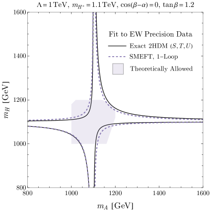
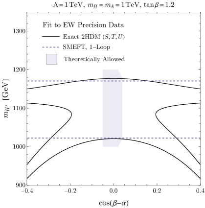
Figure 1: Comparison of constraints on the 2HDM from electroweak precision observables in the full 2HDM (via a fit to the oblique parameters $S$, $T$ and $U$) and in the SMEFT matched to the 2HDM (with loop matching). The region satisfying the theoretical constraints outlined in Section 2.2 is shaded gray.

The left panel considers the alignment limit, $\cos(\beta-\alpha)=0$, and shows an excellent agreement between the full 2HDM results and the results for the SMEFT matched to the 2HDM. The right panel shows $\cos(\beta-\alpha)$ on the horizontal axis. Here, it is again clear that the SMEFT matched to the 2HDM accurately replicates the full 2HDM around the alignment limit. Away from this limit, however, the full 2HDM result changes considerably, whereas the SMEFT matched to the 2HDM does not (as it does not depend on $\cos(\beta-\alpha)$). Finally, both panels show that the SMEFT with one-loop matching provides an excellent description of the full 2HDM in the regions allowed by the theoretical constraints, and for $\cos(\beta-\alpha)\lesssim 0.2$.

In sum, the EWPOs in the 2HDM constitute an example where the SMEFT matched with one-loop dimension-6 operators is clearly more able to accurately replicate the full model than the SMEFT matched with tree-level dimension-8 operators. In fact, whereas the latter do not give a contribution to EWPOs, the former do. On the other hand, this non-zero contribution has no dependence on $\cos(\beta-\alpha)$. This implies that it is adequate for small values of that parameter only, which turn out to be the values preferred by the theoretical constraints.

4.2 Higgs observables

We now turn to Higgs observables. We focus on the Higgs signal strengths measured by ATLAS and CMS. This includes the combined measurements at $\sqrt{s}=7$ and $8\,\textrm{TeV}$ [67], as well as the recent ATLAS and CMS combinations at $\sqrt{s}=13\,\textrm{TeV}$ [68, 69]. Details on the fits can be found in Appendix C.

We start by recapping the results of Ref. [17]. Ignoring for now the indirect effects of the Higgs self-coupling, the only dimension-6 WCs generated via tree-level matching that are relevant for Higgs observables are $C_{f\phi}$ (recall Eq. (20) above). In particular, there is no WC contributing to the Higgs couplings to gauge bosons. Now, considering the first term of the r.h.s of Eqs. (21b) and (21c), as well as Table 1, it is clear that in the Type-I 2HDM, all contributions to $C_{f\phi}$ at $\mathcal{O}(\xi^{1})$ scale as $1/\tan\beta$. The dimension-8 operators, however, include information about Higgs-gauge couplings and $\mathcal{O}(\xi^{2})$ corrections to the $C_{f\phi}$, both of which are independent of $\tan\beta$. Matching up to dimension-8 is thus necessary in the Type-I 2HDM to accurately approximate the full 2HDM for large values of $\tan\beta$. In contrast, in the other types of 2HDM, there is always at least one type of fermion $f$ for which $C_{f\phi}$ at $\mathcal{O}(\xi^{1})$ is not suppressed with $\tan\beta$, so that matching with dimension-8 operators can be neglected in those cases. On the other hand, Ref. [17] showed that Type-F could accommodate, besides a central region centered around $\cos(\beta-\alpha)=0$, also a disjoint region centered around $\cos(\beta-\alpha)\simeq 0.2$ and large values of $\tan\beta$, usually known as the wrong-sign region.

In what follows, we compute the $95\%$ CL limits for Higgs observables, both in the full 2HDM and in the SMEFT matched to the 2HDM. In the full 2HDM, we calculate the observables both at LO and at one-loop (NLO). More specifically, we approximate the NLO results [70, 71, 72, 73, 36, 35] by considering the case near the alignment limit (analytic expressions used to obtain our NLO curves, reproduced from Ref. [70], are given in Appendix A). In the SMEFT matched to the 2HDM, we consider three types of contributions: $d_{6}^{\rm tree}$, $d_{8}^{\rm tree}$ and $d_{6}^{\rm loop}$. The first two consider only the operators generated via tree-level matching, such that $d_{6}^{\rm tree}$ ($d_{8}^{\rm tree}$) includes only $\mathcal{O}(\xi^{1})$ ($\mathcal{O}(\xi^{2})$) effects, while $d_{6}^{\rm loop}$ considers only the contributions generated via one-loop matching at $\mathcal{O}(\xi^{1})$. Note that at $\mathcal{O}(\xi^{2})$ we include $1/\Lambda^{4}$ terms arising from the squared amplitude in our calculation of the signal strengths, which compete with the dimension-8 contributions at the same order.

We now turn to the results of Fig. 2, considering first Type-I (upper left panel).

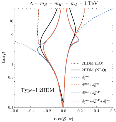
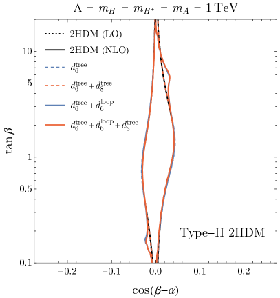
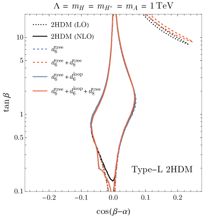
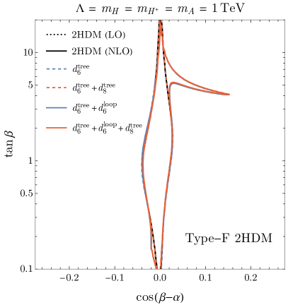
Figure 2: Comparison of the constraints from Higgs precision observables on the 2HDM with the constraints set by a fit to the SMEFT coefficients. The dotted and solid black lines show the constraints in the exact model with the Higgs coupling modifiers evaluated at LO and NLO, respectively (see Appendix A for details). The red and blue lines show the SMEFT result with and without the inclusion of the dimension-eight operators ($d_{8}^{\textrm{tree}}$). The solid red and blue lines include the contributions to the dimension-six operators generated at one-loop in the SMEFT matching ($d_{6}^{\textrm{loop}}$), while the dashed ones do not. In all four panels, the additional heavy states are assumed to be degenerate and equal to the matching scale, $\Lambda$.

Let us start by discussing the results without NLO effects, both in the 2HDM (dotted lines) and in the SMEFT matched to the 2HDM (dashed lines). These results agree with those of Ref. [74]. They present slight differences when compared to those of Ref. [17] (due to the inclusion of new LHC data), but the pattern described above is observed, namely: while the tree-level matching restricted to dimension-6 operators (dashed blue) does not replicate the LO Type-I 2HDM (dotted black) for $\tan\beta>1$, the inclusion of dimension-8 effects (dashed red) corrects that deficiency. The inclusion of NLO effects in the full 2HDM fits (solid black) becomes relevant for $\tan\beta\gtrsim 2$, allowing a considerably more restricted range of values of $\cos(\beta-\alpha)$ for larger values of $\tan\beta$ than the LO result. Interestingly, even if restricted to dimension-6 operators, the SMEFT matched to the 2HDM at one-loop (solid blue) captures the essence of that behavior. This effect is discussed in detail below. Note that adding the dimension-8 tree-level matching to the loop matching with dimension-6 operators does not significantly change the latter.

As for the three remaining panels of Fig. 2, we again confirm what was found in Ref. [17]: if the region centered around $\cos(\beta-\alpha)\sim 0$ is considered at LO, the tree-level matching with dimension-6 operators is enough to replicate the 2HDM result. In fact, the tree-level matching with dimension-6 operators (dashed blue) cannot be distinguished from the tree-level matching with dimension-8 operators (dashed red), nor from the LO 2HDM curve (dotted black). The plots show that the inclusion of loop effects leads to no significant changes either in the full 2HDM results, or in the SMEFT ones. Again as in Ref. [17], Type-L is the only type admitting a wrong-sign region, and only when $\mathcal{O}(\xi^{2})$ effects are included. With this inclusion, and ignoring NLO effects, the SMEFT (dashed red) reproduces quite well the 2HDM (dotted black). On the other hand, the wrong-sign region vanishes from both the 2HDM and the SMEFT descriptions if loop effects (solid lines) are included.

We now discuss the effects observed in the loop matching effects of Type-I. These can be explained by the $C_{f\phi}$ WCs, plotted in the upper half of Fig. 3. In the tree-level matching of Type-I, and as discussed above, they tend to zero at large values of $\tan\beta$. However, in the loop matching and for $\cos(\beta-\alpha)\neq 0$, this behavior is reversed, and the WCs start to grow for $\tan\beta\gtrsim 5$. Note that, even though the sign of $C_{f\phi}$ is the same as that of $\cos(\beta-\alpha)$ for $\tan\beta\lesssim 5$, it always becomes positive for $\tan\beta\gtrsim 5$.

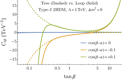
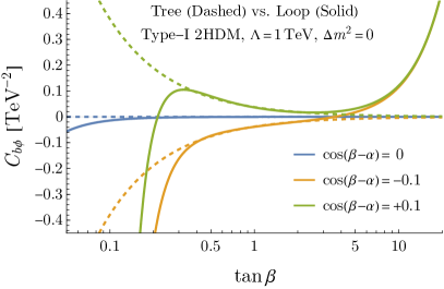
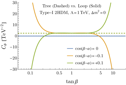
Figure 3: Plots of the WCs $C_{tH}$, $C_{bH}$, and $C_{\phi}$ vs. $\tan\beta$, that are generated in the Type-I 2HDM at tree-level (dashed lines) and one-loop (solid lines), for various values of the alignment parameter, $\cos(\beta-\alpha)$.

In Fig. 3, we also show $C_{\phi}$, although its contributions to Higgs observables are not included in Fig. 2. Like $C_{u\phi}$ and $C_{d\phi}$, it acquires large values (in modulus) for large $\tan\beta$ with loop matching only.

Given the relevance of Type-I for understanding the accuracy of the SMEFT matching to the 2HDM, we explore different features of the Type-I model in Fig. 4. We define $\Delta m^{2}\equiv\Delta m_{H}^{2}=\Delta m_{A}^{2}=\Delta m_{H^{\pm}}^{2}$.

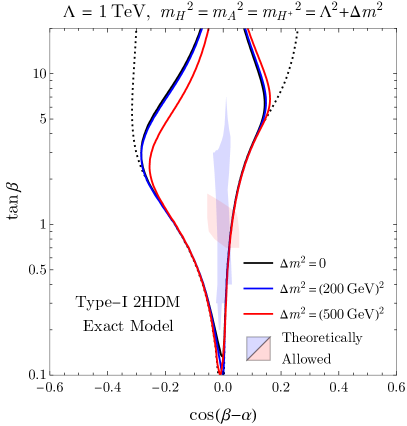
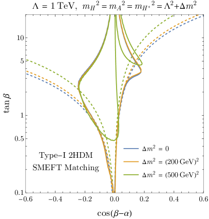
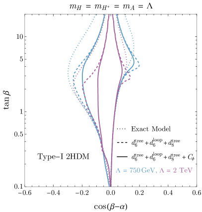
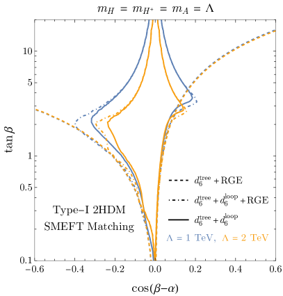
Figure 4: Additional plots showing the constraints from Higgs measurements at the LHC on the fits to the Type-I 2HDM. The upper left panel shows the constraints on the exact model (using the NLO predictions, with the heavy Higgs states separated from the matching scale by various values of $\Delta m^{2}$) and compares these constraints to the theoretically allowed regions described in the text. The LO prediction for the exact model (which does not depend on the mass splitting) is shown as a dashed black curve for comparison. In the upper right panel, we show the same curves, now evaluated using the SMEFT matching at dimension-6 at tree-level (dashed) and one-loop (solid). In the lower left panel, we show the effects of including indirect information from single Higgs production on the Higgs self coupling ($C_{\phi}$) for different values of the matching scale. The lower right panel illustrates the effects of including RGE of the WCs generated at tree-level in the 2HDM, and compares these to the effects of the full contributions generated at one-loop.

In the upper left panel, we consider just the full 2HDM results (not the SMEFT), and investigate both regions of parameter space allowed by theoretical constraints, as well as the dependence on $\Delta m^{2}$. It is clear that the allowed regions are extremely constrained, and forced to be very close to both $\cos(\beta-\alpha)=0$ and $\tan\beta=1$. On the other hand, the 2HDM curves do not depend significantly on $\Delta m^{2}$. The upper right panel considers again the dependence on $\Delta m^{2}$, but now using SMEFT matching to the 2HDM. With tree-level matching, larger values of $\Delta m^{2}$ push the curves upwards in $\tan\beta$. With loop matching, there is little difference between $\Delta m^{2}=0$ and $\Delta m^{2}=(\rm{200\,GeV})^{2}$, but a significant difference for $\Delta m^{2}=(\rm{500\,GeV})^{2}$.

Still in Fig. 4, the lower left panel explores both a dependence on the scale $\Lambda$, as well as the inclusion of $C_{\phi}$ effects (which allow us to indirectly determine the Higgs self-interactions from single Higgs production[76, 77]). As expected, larger values of $\Lambda$ push the results closer to the alignment limit. The inclusion of $C_{\phi}$ effects restricts the results even further. Finally, the lower right panel of Fig. 4 investigates the role of renormalization group evolving the dimension-6 operators between the scales $\Lambda$ and $m_{Z}$. The plot shows that, without loop matching, the RGEs play a very little role (when compared to the dashed blue curve of the upper left panel of Fig. 2), and have a very small dependence on the scale. On the other hand, when loop matching effects are included, the effects of including the RGEs are similar to those of changing $\Lambda$ by a TeV.

5 Conclusions

We have performed for the first time the complete one-loop matching of the 2HDM to the SMEFT with dimension-6 operators. This generates numerous operators not present with the tree-level matching. We derived our result using the software Matchmakereft and Matchete. We obtained agreement in our results between them, which provides a non-trivial check of both software packages. Auxiliary files accompanying this paper include detailed results of the matching.

We demonstrated how the notion of decoupling allowed us to perform a consistent expansion in terms of more physical parameters. This led us to compare the one-loop matching with dimension-6 operators to the tree-level matching with dimension-8 operators derived in Ref. [17]. We did this by performing fits to both EWPOs and to Higgs observables. In the case of EWPOs, while none of the dimension-8 operators generated at tree-level contribute, the dimension-6 loop-generated operators do, thus clearly showing the need for the latter type of matching. In the fits to Higgs observables, we studied the four types of 2HDM and showed that, for Type-II, Type-L and Type-F, the inclusion of higher order effects is not significant, as both the full model 2HDM description and the SMEFT matching to the 2HDM are barely affected by it.

In Type-I, by contrast, the 2HDM results for larger $\tan\beta$ evaluated at NLO are quite different from those evaluated at LO. We showed that the SMEFT matched with loop-generated dimension-6 operators captures most of the physics, and so provides an overall adequate replication of the full model results. We identified the Warsaw basis operators $C_{u\phi}$ and $C_{d\phi}$ as mainly responsible for this phenomenon, as their values at large $\tan\beta$ become quite large with one-loop matching only. We investigated how the results depend on the heavy scale $\Lambda$, on the difference between the heavy masses and $\Lambda$, and on the RGE effects. In all cases, we found significant effects in the region of larger $\tan\beta$.

We note that the difference in the full model between LO and NLO results shows that, in the SMEFT approach, the results obtained with one-loop matching and dimension-6 operators should not be directly compared to those obtained with tree-level matching and dimension-8 operators. Our analysis also shows that, when one requires a separation of scales that allows an EFT description, the 2HDM has a very small region of parameter space allowed by theoretical constraints. In particular, the regions where the non-trivial SMEFT truncations (both at tree-level with dimension-8 operators and at one-loop with dimension-6 operators) become relevant are excluded. On the other hand, matching at one-loop level has been performed in a singlet extension of the SM, only to conclude that it is not relevant in such a simple extension. Both conclusions lead us to suggest an investigation of loop matching in richer UV models, where such matching can play a more decisive role.

Furthermore, although we presented the complete one-loop matching between the 2HDM and the SMEFT with dimension-6 operators, our work represents only a first step towards a complete NLO analysis. Indeed, our analysis includes only approximate expressions of the full NLO 2HDM, and does not contain one-loop correction to the observables computed in the SMEFT. These shortcomings motivate future studies that might ascertain the importance of those corrections.

The auxiliary files for this project can be accessed at the following URL: https://github.com/BDFH-2024/BDFH.

Ackowledgments

We thank Pier Paolo Giardino for discussions. S.D.B. thanks Javier Fuentes-Martín and José Santiago for helping with the SMEFT matching results computation and cross-verification. S.D.B. and D.F. are grateful to the Mainz Institute for Theoretical Physics (MITP) of the Cluster of Excellence PRISMA+ (Project ID 39083149) for its hospitality and support. S.D.B is supported by SRA (Spain) under Grant No. PID2019-106087GB-C21 (10.13039/501100011033) and PID2021-128396NB- 100/AEI/10.13039/501100011033; by the Junta de Andalucía (Spain) under Grants No. FQM-101 and P21_00199. S.D. and D.F. are supported by the U.S. Department of Energy under Grant Contract No. DE-SC0012704. S.H. is supported by the DOE grant DE-SC0013607.

Anexo A More details on the 2HDM

From the minimization of the potential,

$$Y_{1}=-\dfrac{Z_{1}}{2}v^{2},\qquad Y_{3}=-\dfrac{Z_{6}}{2}v^{2}\,.$$ (A.1)

Expressing the $Z_{i}$ parameters of Eq. (10) in terms of the parameters of Eq. (13),

$$Z_{1} = \dfrac{s_{\beta\scalebox{0.5}[0.85]{$-$}\alpha}^{2}m_{h}^{2}+c_{\beta\scalebox{0.5}[0.85]{$-$}\alpha}^{2}\,m_{H}^{2}}{v^{2}},$$

$$Z_{2} = \dfrac{1}{2\,v^{2}\,t_{\beta}^{3}}\bigg{[}c_{\beta\scalebox{0.5}[0.85]{$-$}\alpha}^{2}\,t_{\beta}\left(3t_{\beta}^{4}-8t_{\beta}^{2}+3\right)\left(m_{h}^{2}-m_{H}^{2}\right)+s_{\beta\scalebox{0.5}[0.85]{$-$}\alpha}\,c_{\beta\scalebox{0.5}[0.85]{$-$}\alpha}\big{(}t_{\beta}^{6}-7t_{\beta}^{4}+7t_{\beta}^{2}-1\big{)}\big{(}m_{h}^{2}-m_{H}^{2}\big{)},$$

$$\hskip 36.98857pt-m_{h}^{2}\left(t_{\beta}^{5}-4t_{\beta}^{3}+t_{\beta}\right)+2t_{\beta}\left(t_{\beta}^{2}-1\right)^{2}\left(m_{H}^{2}-Y_{2}\right)\bigg{]},$$

$$Z_{3} = \dfrac{2}{v^{2}}\left(m_{H^{+}}^{2}-Y_{2}\right),$$

$$Z_{4} = \dfrac{c_{\beta\scalebox{0.5}[0.85]{$-$}\alpha}^{2}\left(m_{h}^{2}-m_{H}^{2}\right)+m_{A}^{2}+m_{H}^{2}-2\,m_{H^{+}}^{2}}{v^{2}},$$

$$Z_{5} = \dfrac{c_{\beta\scalebox{0.5}[0.85]{$-$}\alpha}^{2}\left(m_{h}^{2}-m_{H}^{2}\right)-m_{A}^{2}+m_{H}^{2}}{v^{2}},$$

$$Z_{6} = \dfrac{c_{\beta\scalebox{0.5}[0.85]{$-$}\alpha}\,s_{\beta\scalebox{0.5}[0.85]{$-$}\alpha}\,\left(m_{h}^{2}-m_{H}^{2}\right)}{v^{2}},$$

$$Z_{7} = \dfrac{1}{2\,v^{2}\,t_{\beta}^{2}}\bigg{[}-3c_{\beta\scalebox{0.5}[0.85]{$-$}\alpha}^{2}t_{\beta}\left(t_{\beta}^{2}-1\right)\left(m_{h}^{2}-m_{H}^{2}\right)-s_{\beta\scalebox{0.5}[0.85]{$-$}\alpha}c_{\beta\scalebox{0.5}[0.85]{$-$}\alpha}\left(t_{\beta}^{4}-4t_{\beta}^{2}+1\right)\left(m_{h}^{2}-m_{H}^{2}\right),$$ (A.2)

$$\hskip 36.98857pt+t_{\beta}\left(t_{\beta}^{2}-1\right)\left(m_{h}^{2}-2m_{H}^{2}+2Y_{2}\right)\bigg{]}.$$

The effects of the 2HDM on measurements of the $125\,\textrm{GeV}$ Higgs boson production and decay processes can be conveniently parameterized by the so-called “$\kappa$-framework”, where the Higgs couplings to other SM particles are rescaled by Higgs coupling modifiers, $\kappa_{f}$, $\kappa_{V}$ ($V=W,Z$), such that the SM prediction is recovered when $\kappa=1$.

The one-loop (NLO) corrections to the scaling of the Higgs couplings in the 2HDM can be approximated by including contributions which grow with $m_{t}$ and the heavy scalar masses. Working near the decoupling limit, we have [70]

$$\kappa_{V} = s_{\beta\scalebox{0.5}[0.85]{$-$}\alpha}-\frac{1}{6}\frac{1}{16\pi^{2}}\Bigg{[}\frac{m_{H}^{2}}{v^{2}}\Big{(}1-\frac{M^{2}}{m_{H}^{2}}\Big{)}+2\frac{m_{H^{+}}^{2}}{v^{2}}\Big{(}1-\frac{M^{2}}{m_{H^{+}}^{2}}\Big{)}+\frac{m_{A}^{2}}{v^{2}}\Big{(}1-\frac{M^{2}}{m_{A}^{2}}\Big{)}\Bigg{]},$$

$$\kappa_{t} = \kappa_{V}+\frac{\eta_{u}c_{\beta\scalebox{0.5}[0.85]{$-$}\alpha}}{\tan\beta}-\frac{1}{3\tan^{2}\beta}\frac{1}{16\pi^{2}}\Bigg{[}\frac{\eta_{u}^{2}m_{t}^{2}}{v^{2}}\Big{(}\frac{m_{t}^{2}}{m_{H}^{2}}+\frac{m_{t}^{2}}{m_{H^{+}}^{2}}+\frac{m_{t}^{2}}{m_{A}^{2}}\Big{)}+\eta_{d}^{2}\frac{m_{b}^{2}m_{t}^{2}}{v^{2}m_{H^{+}}^{2}}\Bigg{]},$$

$$\kappa_{b} = \kappa_{V}+\frac{\eta_{d}c_{\beta\scalebox{0.5}[0.85]{$-$}\alpha}}{\tan\beta}-\frac{\eta_{u}\eta_{d}}{\tan^{2}\beta}\frac{1}{16\pi^{2}}\frac{4m_{t}^{2}}{v^{2}}\Bigg{[}1-\frac{M^{2}}{m_{H^{+}}^{2}}+\frac{m_{t}^{2}}{m_{H^{+}}^{2}}\Big{(}1+\log\frac{m_{t}^{2}}{m_{H^{+}}^{2}}\Big{)}\Bigg{]}$$

$$\quad-\frac{1}{3}\frac{\eta_{d}^{2}m_{b}^{2}}{v^{2}\tan^{2}\beta}\frac{1}{16\pi^{2}}\bigg{(}\frac{m_{b}^{2}}{m_{H}^{2}}+\frac{m_{b}^{2}}{m_{H^{+}}^{2}}+\frac{m_{b}^{2}}{m_{A}^{2}}\bigg{)},$$

$$\kappa_{\tau} = \kappa_{V}+\frac{\eta_{e}c_{\beta\scalebox{0.5}[0.85]{$-$}\alpha}}{\tan\beta},$$ (A.3)

where

$$M^{2}=Y_{2}-Y_{1}-2Y_{3}\tan 2\beta,$$ (A.4)

is the scale that describes the soft-breaking of the $\mathbb{Z}_{2}$ symmetry. We emphasize again that these are not the complete expressions for the loop corrections to the Higgs couplings, only the leading terms in an expansion in $x\equiv\pi/2-(\beta-\alpha)\ll 1$. In particular, we keep only the $x$-independent one-loop corrections. See Ref. [70] for more details.

Anexo B One-loop matching results

In this appendix, we present the matching expressions for the SMEFT coefficients of Eq. (24). As discussed in Section 3.1, because these coefficients are loop generated, we expand them only to $\mathcal{O}(\xi^{1})$. We recall (Eq. (17)) that, for operators that are not generated at tree-level, we write the coefficients as $C_{i}$ (without superscript $[l]$). For operators that are generated at tree-level, $C_{\phi}$ and $C_{f\phi}$, we give the one-loop contributions, $C_{\phi}^{[l]}$ and $C_{f\phi}^{[l]}$, here, which must be added to the dimension-6 tree-level contributions,$C_{\phi}^{[t]}$ and $C_{f\phi}^{[t]}$, of Eq. (21) to obtain the full results. As always, the generation indices are suppressed.

The results are:

$$\dfrac{C_{\phi W}}{\Lambda^{2}} = \dfrac{m_{W}^{2}\,G_{F}^{2}}{96\,\pi^{2}\,\Lambda^{2}}\left(\Delta m_{A}^{2}+\Delta m_{H}^{2}+2\,\Delta m_{H^{+}}^{2}\right),$$ (B.5a)

$$\dfrac{C_{\phi B}}{\Lambda^{2}} = \dfrac{G_{F}^{2}}{96\,\pi^{2}\,\Lambda^{2}}(m_{Z}^{2}-m_{W}^{2})\left(\Delta m_{A}^{2}+\Delta m_{H}^{2}+2\,\Delta m_{H^{+}}^{2}\right),$$ (B.5b)

$$\dfrac{C_{\phi WB}}{\Lambda^{2}} = \dfrac{G_{F}^{2}{m_{W}}\,{m_{Z}}}{48\,\pi^{2}\,\Lambda^{2}}\sqrt{1-\dfrac{m_{W}^{2}}{m_{Z}^{2}}}\left(\Delta m_{A}^{2}+\Delta m_{H}^{2}-2\,\Delta m_{H^{+}}^{2}\right),$$ (B.5c)

$$\dfrac{C_{\phi}^{[l]}}{\Lambda^{2}} = -\dfrac{(\sqrt{2}G_{F})^{3}\,\cot^{3}\beta}{480\,\pi^{2}\,\Lambda^{2}}\Bigg{\{}-\dfrac{45}{2}\,c_{\beta\scalebox{0.5}[0.85]{$-$}\alpha}^{3}\,\Lambda^{6}\left(\cos(2\,{\beta})+\cos(6\,{\beta})\right)\sec^{6}\beta$$ (B.5d)

$$+2\,\bigg{(}10\left(\Delta m_{A}^{6}+\Delta m_{H}^{6}+2\,\Delta m_{H^{+}}^{6}\right)-5\,\Big{[}\Delta m_{A}^{4}+\Delta m_{H}^{4}-2\left(\Delta m_{A}^{2}+\Delta m_{H}^{2}\right)\,\Delta m_{H^{+}}^{2}$$

$$+2\,\Delta m_{H^{+}}^{4}\Big{]}\,m_{h}^{2}+2\,m_{h}^{2}\,m_{W}^{4}\bigg{)}\tan^{3}\beta+15\,c_{\beta\scalebox{0.5}[0.85]{$-$}\alpha}^{2}\,\Lambda^{4}\,\tan\beta\Big{[}m_{h}^{2}\left(-5+2\,\cos(4\,{\beta})\right)\,\sec^{4}\beta$$

$$+6\,\Delta m_{H}^{2}\left(-1+\sec^{2}\beta+\sec^{4}\beta\right)-2\left(\Delta m_{A}^{2}+2\,\Delta m_{H^{+}}^{2}\right)\,\tan^{2}\beta\Big{]}$$

$$-90\,c_{\beta\scalebox{0.5}[0.85]{$-$}\alpha}\,\Lambda^{2}\left(-2\,\Delta m_{H}^{2}+m_{h}^{2}\right)^{2}\,\tan^{2}\beta\left(\tan^{2}({\beta})-1\right)\Bigg{\}},$$

$$\dfrac{C_{\phi\Box}}{\Lambda^{2}} = -\dfrac{G_{F}^{2}}{480\,\pi^{2}\,\Lambda^{2}}\,\Big{[}-5\left(\Delta m_{A}^{2}-\Delta m_{H}^{2}\right)^{2}+20\left(\Delta m_{A}^{2}+\Delta m_{H}^{2}\right)\,\Delta m_{H^{+}}^{2}$$ (B.5e)

$$\hskip 68.2866pt+2\left(45\,c_{\beta\scalebox{0.5}[0.85]{$-$}\alpha}^{2}\,\Lambda^{4}+4\,m_{W}^{4}-2\,m_{W}^{2}\,m_{Z}^{2}+m_{Z}^{4}\right)\Big{]},$$

$$\dfrac{C_{\phi D}}{\Lambda^{2}} = -\dfrac{G_{F}^{2}}{60\,\pi^{2}\,\Lambda^{2}}\,\Big{[}-5\,\Delta m_{H}^{2}\,\Delta m_{H^{+}}^{2}+5\,\Delta m_{H^{+}}^{4}+5\,\Delta m_{A}^{2}\left(\Delta m_{H}^{2}-\Delta m_{H^{+}}^{2}\right)$$ (B.5f)

$$\hskip 68.2866pt+m_{W}^{4}-2\,m_{W}^{2}\,m_{Z}^{2}+m_{Z}^{4}\Big{]},$$

$$\dfrac{C_{u\phi}^{[l]}}{\Lambda^{2}} = \dfrac{{m_{u}}\,(\sqrt{2}G_{F})^{5/2}}{\sqrt{2}\,480\,\pi^{2}\,\Lambda^{2}}\Bigg{\{}10\,\Big{[}\Delta m_{A}^{4}+(1-36\eta_{u})\,\Delta m_{H}^{4}-2\,\Delta m_{A}^{2}\,\Delta m_{H^{+}}^{2}+2\,\Delta m_{H^{+}}^{4}-9\,\eta_{u}\,m_{h}^{4}$$ (B.5g)

$$-(30+63\eta_{u})\,c_{\beta\scalebox{0.5}[0.85]{$-$}\alpha}^{2}\,\Lambda^{4}-2\,\Delta m_{H}^{2}\left(\Delta m_{H^{+}}^{2}-18\eta_{u}\,m_{h}^{2}\right)\Big{]}-30\,c_{\beta\scalebox{0.5}[0.85]{$-$}\alpha}\cot\beta\,\Lambda^{2}\,\Big{(}2\,\eta_{u}\,\Delta m_{A}^{2}$$

$$-6(1+\eta_{u})\,\Delta m_{H}^{2}+4\,\eta_{u}\,\Delta m_{H^{+}}^{2}-\,m_{d}^{2}(3\eta_{d}+4\eta_{u})+3\,m_{h}^{2}+13\,\eta_{u}\,m_{u}^{2}\Big{)}-4\,m_{W}^{4}$$

$$+10\,\cot^{2}\beta\,\Big{[}6\big{(}6\,\eta_{u}\,\Delta m_{H}^{4}+\frac{3}{2}\,(1+7\eta_{u})\,c_{\beta\scalebox{0.5}[0.85]{$-$}\alpha}^{2}\,\Lambda^{4}+\eta_{d}(4\eta_{u}-\eta_{d})\,\Delta m_{H^{+}}^{2}\,m_{d}^{2}$$

$$-\eta_{d}(\eta_{d}+4\eta_{u})\,m_{d}^{4}\big{)}+9\left(-4\,\eta_{u}\,\Delta m_{H}^{2}+\eta_{u}\eta_{d}m_{d}^{2}\right)\,m_{h}^{2}+9\eta_{u}\,m_{h}^{4}$$

$$-2\,\eta_{u}^{2}\left(-3\,\Delta m_{A}^{2}+9\,\Delta m_{H}^{2}+3\,\Delta m_{H^{+}}^{2}\right)\,m_{u}^{2}-2(6\eta_{d}\eta_{u}+3\eta_{u}^{2}-\eta_{d}^{2})m_{d}^{2}m_{u}^{2}-6\eta_{u}^{2}\,m_{u}^{4}\Big{]}$$

$$+15\eta_{u}\,c_{\beta\scalebox{0.5}[0.85]{$-$}\alpha}\,\Lambda^{2}\left(-7\eta_{d}^{2}\,m_{d}^{2}+3\eta_{u}^{2}\,m_{u}^{2}\right)\cot^{3}\beta-90\eta_{u}\,c_{\beta\scalebox{0.5}[0.85]{$-$}\alpha}^{2}\,\Lambda^{4}\,\cot^{4}\beta$$

$$+90\,c_{\beta\scalebox{0.5}[0.85]{$-$}\alpha}\Lambda^{2}\tan({\beta})\Big{[}-2\Delta m_{H}^{2}+m_{h}^{2}+(1+\eta_{u})c_{\beta\scalebox{0.5}[0.85]{$-$}\alpha}\Lambda^{2}\tan({\beta})\Big{]}\Bigg{\}},$$

$$\dfrac{C_{d\phi}^{[l]}}{\Lambda^{2}} = \dfrac{{m_{d}}\,(\sqrt{2}G_{F})^{5/2}}{\sqrt{2}\,480\,\pi^{2}\,\Lambda^{2}}\bigg{\{}10\,\Big{[}\Delta m_{A}^{4}+(1-36\eta_{d})\,\Delta m_{H}^{4}-2\,\Delta m_{A}^{2}\,\Delta m_{H^{+}}^{2}+2\,\Delta m_{H^{+}}^{4}$$ (B.5h)

$$-(30+63\eta_{d})\,c_{\beta\scalebox{0.5}[0.85]{$-$}\alpha}^{2}\,\Lambda^{4}-9\eta_{d}\,m_{h}^{4}-2\,\Delta m_{H}^{2}\left(\Delta m_{H^{+}}^{2}-18\,\eta_{d}\,m_{h}^{2}\right)\Big{]}-4\,m_{W}^{4}$$

$$-30\,c_{\beta\scalebox{0.5}[0.85]{$-$}\alpha}\,\Lambda^{2}\,\cot\beta\,\Big{(}2\eta_{d}\,\Delta m_{A}^{2}-6(1+\eta_{d})\,\Delta m_{H}^{2}+4\eta_{d}\,\Delta m_{H^{+}}^{2}+13\eta_{d}\,m_{d}^{2}+3\,m_{h}^{2}$$

$$-(4\eta_{d}+3\eta_{u})\,m_{u}^{2}\Big{)}+10\,\cot^{2}\beta\,\Big{[}36\eta_{d}\,\Delta m_{H}^{4}+9(1+7\eta_{d})\,c_{\beta\scalebox{0.5}[0.85]{$-$}\alpha}^{2}\,\Lambda^{4}+9\eta_{d}\,m_{h}^{4}$$

$$-6\eta_{d}^{2}\,m_{d}^{2}\left(-\Delta m_{A}^{2}+\Delta m_{H^{+}}^{2}+m_{d}^{2}\right)-18\eta_{d}\,\Delta m_{H}^{2}\left(m_{d}^{2}\eta_{d}+2\,m_{h}^{2}\right)-6(\eta_{u}^{2}+4\eta_{d}\eta_{u})\,m_{u}^{4}$$

$$+\big{(}6\eta_{u}(4\eta_{d}-\eta_{u})\,\Delta m_{H^{+}}^{2}+2(\eta_{u}^{2}-6\eta_{u}\eta_{d}-3\eta_{d}^{2})\,m_{d}^{2}+9\eta_{d}\eta_{u}\,m_{h}^{2}\big{)}\,m_{u}^{2}\Big{]}$$

$$+15\eta_{d}\,c_{\beta\scalebox{0.5}[0.85]{$-$}\alpha}\,\Lambda^{2}\left(3\eta_{d}^{2}\,m_{d}^{2}-7\eta_{u}^{2}\,m_{u}^{2}\right)\,\cot^{3}\beta-90\eta_{d}\,c_{\beta\scalebox{0.5}[0.85]{$-$}\alpha}^{2}\,\Lambda^{4}\,\cot^{4}\beta$$

$$+90\,c_{\beta\scalebox{0.5}[0.85]{$-$}\alpha}\,\Lambda^{2}\,\tan\beta\left(-2\,\Delta m_{H}^{2}+m_{h}^{2}+(1+\eta_{d})\,c_{\beta\scalebox{0.5}[0.85]{$-$}\alpha}\,\Lambda^{2}\,\tan({\beta})\right)\bigg{\}},$$

$$\dfrac{C_{e\phi}^{[l]}}{\Lambda^{2}} = \dfrac{{m_{e}}\,(\sqrt{2}G_{F})^{5/2}}{\sqrt{2}\,240\,\pi^{2}\,\Lambda^{2}}\bigg{\{}5\Delta m_{A}^{4}-10\Delta m_{A}^{2}\Delta m_{H^{+}}^{2}+10\Delta m_{H^{+}}^{4}-2m_{W}^{4}$$ (B.5i)

$$-15\,c_{\beta\scalebox{0.5}[0.85]{$-$}\alpha}\,\Lambda^{2}\,\cot\beta\Big{(}6\Delta m_{H}^{2}(-1+\tan^{2}\beta-\eta_{e})-3m_{h}^{2}(-1+\tan^{2}\beta)$$

$$+2\eta_{e}(\Delta m_{A}^{2}+2\Delta m_{H^{+}}^{2})\Big{)}-10\Delta m_{H}^{2}\Big{(}\Delta m_{H^{+}}^{2}-18m_{h}^{2}(-1+\tan^{2}\beta)\eta_{e}\cot^{2}\beta\Big{)}$$

$$+15c_{\beta\scalebox{0.5}[0.85]{$-$}\alpha}^{2}\Lambda^{4}\Big{(}-3\eta_{e}\cot^{4}\beta+3\tan^{2}\beta(1+\eta_{e})+3(1+7\eta_{e})\cot^{2}\beta\Big{.}\Big{.}-(10+21\eta_{e})\Big{)}$$

$$+45m_{h}^{4}\eta_{e}\cot^{2}\beta-45m_{h}^{4}\eta_{e}+5\Delta m_{H}^{4}\Big{(}(1-36\eta_{e})+36\eta_{e}\cot^{2}\beta\Big{)}\bigg{\}},$$

$$\dfrac{C_{\phi u}}{\Lambda^{2}} = \dfrac{G_{F}^{2}}{1080\,\pi^{2}\,\Lambda^{2}}\,\Big{[}-12\left(m_{W}^{2}-m_{Z}^{2}\right)^{2}+\left\{5\,\eta_{u}^{2}\,m_{u}^{2}\left(-63\,m_{u}^{2}+10\,m_{W}^{2}-10\,m_{Z}^{2}\right)\right.$$ (B.5j)

$$\hskip 68.2866pt\left.-45\,m_{u}^{2}m_{d}^{2}\left(\eta_{d}^{2}-6\eta_{d}\eta_{u}-6\eta_{u}^{2}\right)\right\}\,\cot^{2}\beta\Big{]},$$

$$\dfrac{C_{\phi d}}{\Lambda^{2}} = \dfrac{G_{F}^{2}}{1080\,\pi^{2}\,\Lambda^{2}}\,\Big{[}6\left(m_{W}^{2}-m_{Z}^{2}\right)^{2}+\left\{5\,\eta_{d}^{2}\,m_{d}^{2}\left(63\,m_{d}^{2}+22\,m_{W}^{2}-22\,m_{Z}^{2}\right)\right.$$ (B.5k)

$$\hskip 68.2866pt\left.+45\,m_{d}^{2}\,m_{u}^{2}\left(-6\eta_{d}^{2}-6\eta_{u}\eta_{d}+\eta_{u}^{2}\right)\right\}\,\cot^{2}\beta\Big{]},$$

$$\dfrac{C_{\phi l}}{\Lambda^{2}} = \dfrac{G_{F}^{2}}{360\,\pi^{2}\,\Lambda^{2}}\left(6\left(m_{W}^{2}-m_{Z}^{2}\right)^{2}+35\,\eta_{e}^{2}\,m_{e}^{2}\left(3\,m_{e}^{2}-2\,m_{W}^{2}+2\,m_{Z}^{2}\right)\,\cot^{2}\beta\right),$$ (B.5l)

$$\dfrac{C_{\phi q}^{(1)}}{\Lambda^{2}} = -\dfrac{G_{F}^{2}}{1080\,\pi^{2}\,\Lambda^{2}}\bigg{\{}3\left(m_{W}^{2}-m_{Z}^{2}\right)^{2}+5\cot^{2}\beta\Big{[}63\,\eta_{d}^{2}\,m_{d}^{4}$$ (B.5m)

$$\hskip 68.2866pt-7\,\eta_{u}^{2}\,m_{u}^{2}\left(9\,m_{u}^{2}+5\,m_{W}^{2}-5\,m_{Z}^{2}\right)+19\,\eta_{d}^{2}\,m_{d}^{2}\left(m_{W}^{2}-m_{Z}^{2}\right)\Big{]}\bigg{\}},$$

$$\dfrac{C_{\phi q}^{(3)}}{\Lambda^{2}} = \dfrac{G_{F}^{2}}{360\,\pi^{2}\,\Lambda^{2}}\bigg{(}5\cot^{2}\beta\Big{[}-3\left(\eta_{d}^{2}\,m_{d}^{4}-6\,\eta_{d}\,\eta_{u}\,\,m_{d}^{2}\,m_{u}^{2}+\eta_{u}^{2}\,m_{u}^{4}\right)$$ (B.5n)

$$\hskip 68.2866pt+\left(\eta_{d}^{2}\,m_{d}^{2}+\eta_{u}^{2}\,m_{u}^{2}\right)\,m_{W}^{2}\Big{]}-3m_{W}^{4}\bigg{)},$$

$$\dfrac{C_{\phi l}^{(1)}}{\Lambda^{2}} = \dfrac{G_{F}^{2}}{360\,\pi^{2}\,\Lambda^{2}}\Big{[}3\left(m_{W}^{2}-m_{Z}^{2}\right)^{2}-5\,m_{e}^{2}\,\eta_{e}^{2}\,\left(21\,m_{e}^{2}+17\left(m_{W}^{2}-m_{Z}^{2}\right)\right)\,\cot^{2}\beta\Big{]},$$ (B.5o)

$$\dfrac{C_{\phi l}^{(3)}}{\Lambda^{2}} = -\dfrac{G_{F}^{2}}{360\,\pi^{2}\,\Lambda^{2}}\Big{[}3\,m_{W}^{4}+5\,m_{e}^{2}\eta_{e}^{2}\left(3\,m_{e}^{2}-m_{W}^{2}\right)\,\cot^{2}\beta\Big{]},$$ (B.5p)

$$\dfrac{C_{\bm{ll}}}{\Lambda^{2}} = -\dfrac{m_{W}^{4}\,G_{F}^{2}}{120\,\pi^{2}\,\Lambda^{2}}.$$ (B.5q)

Anexo C Higgs observables to $\mathcal{O}(\xi^{2})$

Here we summarize the dependence of the Higgs signal strengths on the various WCs generated in the 2HDM. We include the dependence on coefficients up to $\mathcal{O}(\xi^{2})$, generated at tree-level, as well as those generated at one-loop at $\mathcal{O}(\xi^{1})$. We emphasize that these expressions do not include the most general dependence on the SMEFT coefficients, regardless of flavor ansatz, as we omit any operators that are not generated in the 2HDM, which are irrelevant for our analysis.

We consider the signal strengths for Higgs production in gluon-gluon fusion (ggF), vector boson-fusion (VBF), associated production with a $W$ or $Z$ boson ($Wh$ and $Zh$), and $t\bar{t}h$ production. We neglect any SMEFT deviations in the single-top ($th$) production mode, which is often measured together with $t\bar{t}h$ production, and assume that the $t\bar{t}h$ contribution is dominant. The signal strengths for Higgs production are defined as $\mu_{\textrm{prod}}=\sigma_{\textrm{prod}}^{\textsc{SMEFT}}/\sigma_{\textrm{prod}}^{\textsc{SM}}$, where $\sigma_{\textrm{prod}}^{\textsc{SM}}$ is the SM value. When multiple production channels are combined into a single measurement, we take the signal strength to be the average of the two channels, weighted by their relative SM predictions from Ref. [78]. We indicate $8\,\textrm{TeV}$ or $13\,\textrm{TeV}$ for the signal strengths that depend on the collider energy.

The signal strengths of the decays shown are the same ratio with the partial widths evaluated in the SMEFT and in the SM. We consider Higgs decays to $b\bar{b}$, $WW^{*}(\to\ell\nu\ell\nu)$, $gg$, $\tau^{+}\tau^{-}$, $ZZ^{*}(\to 4\ell)$, $\gamma\gamma$, $Z\gamma$ and $\mu^{+}\mu^{-}$. For all the decays involving either on- or off-shell $Z$ and $W$’s, we neglect any effective operators appearing in the $Z,W\to f\bar{f}$ vertex, so that, e.g., $\mu_{h\to 4\ell}=\mu_{h\to\ell^{+}\ell^{-}\nu\bar{\nu}}=\mu_{h\to\ell^{+}\ell^{-}q\bar{q}}\equiv\mu_{h\to ZZ^{*}}$. The signal strengths for the individual decay modes can be combined with the known, SM branching ratios (BRs) for the Higgs to get the signal strength for the total width,

$$\mu_{\Gamma_{h,\textrm{tot.}}}=\sum_{X}\,\mu_{h\to X}\times\textrm{BR}(h\to X)_{\textsc{SM}},$$ (C.6)

which can then be used to predict the individual BRs in the SMEFT. We take the predictions for the SM branching ratios from Ref. [78].

In computing the coefficients below, we use $G_{F}=1.1663787\times 10^{-5}\,\textrm{GeV}^{-2}$, $m_{Z}=91.1876\,\textrm{GeV}$, $m_{W}=80.379\,\textrm{GeV}$, $m_{h}=125.0\,\textrm{GeV}$, $m_{t}=173\,\textrm{GeV}$, $m_{b}=4.18\,\textrm{GeV}$ and $m_{\tau}=1.776\,\textrm{GeV}$. We keep only the masses of the third generation fermions, and set the first and second generation masses to zero. The WCs are given in units of $\textrm{TeV}^{-2}$ for the dimension-six operators, and $\textrm{TeV}^{-4}$ for those at dimension-eight. The signal strengths for $h\rightarrow 4\ell$ are taken from Ref. [79] to account for the effects of experimental efficiencies, while the others are computed analytically at leading order.

C.1 Production

$$\mu_{\textrm{ggF}} = 1+0.249\,C_{d\phi,33}+0.121\,C_{\phi\Box}-0.129\,C_{u\phi,33}-0.0606\,C_{\phi l,11}^{(3)}-0.0606\,C_{\phi l,22}^{(3)}$$ (C.7a)

$$\quad+\;0.0606\,C_{\bm{ll}}-0.0303\,C_{\phi D}+0.0540\,(C_{d\phi,33})^{2}-0.0182\,C_{d\phi,33}\,C_{u\phi,33}$$

$$\quad+\;0.00421\,C_{u\phi,33}^{2}+0.0151\,C_{qd\phi^{5},33}-0.00784\,C_{qu\phi^{5},33},$$

$$\mu_{\textsc{vbf}}^{\textrm{8\,TeV}} = 1-0.370\,C_{\phi q,11}^{(3)}-0.344\,C_{\bm{\phi l}}^{(3)}+0.113\,C_{\phi\Box}+0.0825\,C_{\bm{ll}}$$ (C.7b)

$$\quad-\;0.0533\,C_{\phi W}+0.0238\,C_{\phi WB}-0.0148\,C_{\phi u,11}+0.0112\,C_{\phi q,11}^{(1)}$$

$$\quad-\;0.0106\,C_{\phi D}+0.00353\,C_{\phi d,11}-0.00304\,C_{\phi B}+0.000392\,C_{\phi^{6}}^{(1)},$$

$$\mu_{\textsc{vbf}}^{\textrm{13\,TeV}} = 1-0.423\,C_{\phi q,11}^{(3)}-0.347\,C_{\phi q,11}^{(3)}+0.1005\,C_{\phi\Box}+0.0826\,C_{\bm{ll}}$$ (C.7c)

$$\quad-\;0.0670\,C_{\phi W}-0.02955\,C_{\phi u,11}-0.0150\,C_{\phi D}+0.0126\,C_{\phi WB}$$

$$\quad-\;0.0107\,C_{\phi B}+0.00893\,C_{\phi q,11}^{(1)}+0.00313\,C_{\phi d,11}+0.000490\,C_{\phi^{6}}^{(1)},$$

$$\mu_{Wh}^{\textrm{8\,TeV}} = 1+1.819\,C_{\phi q,11}^{(3)}+0.8775\,C_{\phi W}+0.1214\,C_{\phi\Box}+0.0602\,C_{\bm{ll}}$$ (C.7d)

$$\quad-\;0.0309\,C_{\phi D}-7.916\times 10^{-6}\,C_{\phi^{6}}^{(1)},$$

$$\mu_{Wh}^{\textrm{13\,TeV}} = 1+1.950\,C_{\phi q,11}^{(3)}+0.887\,C_{\phi W}+0.1217\,C_{\phi\Box}+0.0606\,C_{\bm{ll}}$$ (C.7e)

$$\quad-\;0.0303\,C_{\phi D}-4.326\times 10^{-6}\,C_{\phi^{6}}^{(1)},$$

$$\mu_{Zh}^{\textrm{8\,TeV}} = 1+1.716\,C_{\phi q,11}^{(3)}+0.721\,C_{\phi W}+0.426\,C_{\phi u,11}+0.314\,C_{\phi WB}-0.173\,C_{\phi q,11}^{(1)}$$ (C.7f)

$$\quad-\;0.142\,C_{\phi d,11}+0.121\,C_{\phi\Box}+0.0865\,C_{\phi B}+0.06045\,C_{\bm{ll}}+0.0375\,C_{\phi D}$$

$$\quad-\;3.515\times 10^{-6}\,C_{\phi^{6}}^{(1)},$$

$$\mu_{Zh}^{\textrm{13\,TeV}} = 1+1.716\,C_{\phi q,11}^{(3)}+0.721\,C_{\phi W}+0.426\,C_{\phi u,11}-0.173\,C_{\phi q,11}^{(1)}-0.142\,C_{\phi d,11}$$ (C.7g)

$$\quad+\;0.121\,C_{\phi\Box}+0.0865\,C_{\phi B}+0.0375\,C_{\phi D}+0.314\,C_{\phi WB}+0.06045\,C_{\bm{ll}}$$

$$\quad-\;3.515\times 10^{-6}\,C_{\phi^{6}}^{(1)},$$

$$\mu_{t\bar{t}h} = 1+0.121\,C_{\phi\Box}-0.122\,C_{u\phi,33}-0.0606\,C_{\phi l,11}^{(3)}-0.0606\,C_{\phi l,22}^{(3)}+0.0606\,C_{\bm{ll}}$$ (C.7h)

$$\quad-\;0.0303\,C_{\phi D}-0.00740\,C_{qu\phi^{5},33}+0.00372\,(C_{u\phi,33})^{2}.$$

C.2 Decays

$$\mu_{h\to b\bar{b}} = 1-5.050\,C_{d\phi,33}+0.121\,{C_{\phi\Box}}-0.121\,{C_{\bm{\phi l}}^{(3)}}-0.0303\,{C_{\phi D}}+0.0606\,{C_{\bm{ll}}},$$ (C.8a)

$$\quad+\;6.376\,(C_{d\phi,33})^{2}-0.306\,C_{qd\phi^{5},33},$$

$$\mu_{h\to WW^{*}} = 1+0.1202\,{C_{\phi\Box}}+0.0935\,{C_{\bm{ll}}}-0.0895\,C_{\phi W}-0.0297\,{C_{\phi D}}+0.000507\,C_{\phi^{6}}^{(1)},$$ (C.8b)

$$\mu_{h\to gg} = 1+0.249\,C_{d\phi,33}-0.129\,C_{u\phi,33}+0.1225\,{C_{\phi\Box}}+0.0613\,{C_{\bm{ll}}}-0.0306\,{C_{\phi D}}$$ (C.8c)

$$\quad+\;0.054\,(C_{d\phi,33})^{2}-0.0182\,C_{d\phi,33}\,C_{u\phi,33}+0.0042\,C_{u\phi,33}^{2}$$

$$\quad-\;0.0078\,C_{qu\phi^{5},33}+0.0151\,C_{qd\phi^{5},33},$$

$$\mu_{h\to\tau^{+}\tau^{-}} = 1-11.88\,{C_{e\phi,33}}+0.121\,{C_{\phi\Box}}-0.121\,{C_{\bm{\phi l}}^{(3)}}+0.0606\,{C_{\bm{ll}}}-0.0303\,{C_{\phi D}}$$ (C.8d)

$$\quad+\;35.29\,(C_{e\phi,33})^{2}-0.720\,{C_{e\phi^{5},33}},$$

$$\mu_{h\to ZZ^{*}} = 1+0.296\,C_{\phi WB}-0.296\,C_{\phi W}-0.234\,C_{\bm{\phi l}}^{(3)}-0.197\,C_{\phi B}+0.181\,C_{\bm{ll}}$$ (C.8e)

$$\quad+\;0.119\,C_{\phi\Box}+0.126\,C_{\phi l,11}^{(1)}-0.101\,C_{\phi l,11}+0.005\,C_{\phi D},$$

$$\mu_{h\to\gamma\gamma} = 1-40.15\,C_{\phi B}+22.30\,C_{\phi WB}-13.08\,C_{\phi W}-0.364\,C_{\phi l,11}^{(3)}-0.242\,C_{\phi D}$$ (C.8f)

$$\quad+\;0.182\,C_{\bm{ll}}+0.121\,C_{\phi\Box}+0.0345\,C_{u\phi,33},$$

$$\mu_{h\to Z\gamma} = 1-15.47\,C_{\phi B}+14.58\,C_{\phi W}-11.04\,C_{\phi WB}-0.182\,C_{\bm{\phi l}}^{(3)}$$ (C.8g)

$$\quad+\;0.1215\,C_{\phi\Box}-0.121\,C_{\phi D}+0.0177\,C_{\phi q,11}^{(1)}-0.0177\,C_{\phi q,11}^{(3)}+0.0177\,C_{\phi u,11}$$

$$\quad+\;0.0909\,C_{\bm{ll}}+0.00721\,C_{u\phi,33}+0.00184\,C_{\phi^{6}}^{(1)}+0.000437\,C_{qu\phi^{5},33},$$

$$\mu_{h\to\mu^{+}\mu^{-}} = 1-199.79\,C_{e\phi,22}+0.121\,{C_{\phi\Box}}-0.121\,{C_{\bm{\phi l}}^{(3)}}+0.0606\,{C_{\bm{ll}}}-0.0303\,{C_{\phi D}}$$ (C.8h)

$$\quad+\;9978.95\,(C_{e\phi,22})^{2}-12.11\,C_{e\phi^{5},22}.$$

References

- [1] I. Brivio and M. Trott, “The Standard Model as an Effective Field Theory,” Phys. Rept. 793 (2019) 1–98, arXiv:1706.08945 [hep-ph].
- [2] G. Isidori, F. Wilsch, and D. Wyler, “The Standard Model effective field theory at work,” arXiv:2303.16922 [hep-ph].
- [3] B. Henning, X. Lu, and H. Murayama, “How to use the Standard Model effective field theory,” JHEP 01 (2016) 023, arXiv:1412.1837 [hep-ph].
- [4] M. Gorbahn, J. M. No, and V. Sanz, “Benchmarks for Higgs Effective Theory: Extended Higgs Sectors,” JHEP 10 (2015) 036, arXiv:1502.07352 [hep-ph].
- [5] M. Jiang, N. Craig, Y.-Y. Li, and D. Sutherland, “Complete one-loop matching for a singlet scalar in the Standard Model EFT,” JHEP 02 (2019) 031, arXiv:1811.08878 [hep-ph]. [Erratum: JHEP 01, 135 (2021)].
- [6] U. Haisch, M. Ruhdorfer, E. Salvioni, E. Venturini, and A. Weiler, “Singlet night in Feynman-ville: one-loop matching of a real scalar,” JHEP 04 (2020) 164, arXiv:2003.05936 [hep-ph]. [Erratum: JHEP 07, 066 (2020)].
- [7] S. Dawson, S. Homiller, and S. D. Lane, “Putting standard model EFT fits to work,” Phys. Rev. D 102 no. 5, (2020) 055012, arXiv:2007.01296 [hep-ph].
- [8] S. Das Bakshi, J. Chakrabortty, C. Englert, M. Spannowsky, and P. Stylianou, “ violation at ATLAS in effective field theory,” Phys. Rev. D 103 no. 5, (2021) 055008, arXiv:2009.13394 [hep-ph].
- [9] R. Contino, A. Falkowski, F. Goertz, C. Grojean, and F. Riva, “On the Validity of the Effective Field Theory Approach to SM Precision Tests,” JHEP 07 (2016) 144, arXiv:1604.06444 [hep-ph].
- [10] H. Bélusca-Maïto, Search for new physics at the LHC using Higgs Effective Field Theory. PhD thesis, Orsay, 3, 2016.
- [11] J. Ellis, S.-F. Ge, H.-J. He, and R.-Q. Xiao, “Probing the scale of new physics in the coupling at colliders,” Chin. Phys. C 44 no. 6, (2020) 063106, arXiv:1902.06631 [hep-ph].
- [12] C. W. Murphy, “Dimension-8 operators in the Standard Model Eective Field Theory,” JHEP 10 (2020) 174, arXiv:2005.00059 [hep-ph].
- [13] T. Corbett, A. Helset, A. Martin, and M. Trott, “EWPD in the SMEFT to dimension eight,” JHEP 06 (2021) 076, arXiv:2102.02819 [hep-ph].
- [14] C. Degrande and H.-L. Li, “Impact of dimension-8 SMEFT operators on diboson productions,” JHEP 06 (2023) 149, arXiv:2303.10493 [hep-ph].
- [15] T. Corbett, J. Desai, O. J. P. Éboli, M. C. Gonzalez-Garcia, M. Martines, and P. Reimitz, “Impact of dimension-eight SMEFT operators in the electroweak precision observables and triple gauge couplings analysis in universal SMEFT,” Phys. Rev. D 107 no. 11, (2023) 115013, arXiv:2304.03305 [hep-ph].
- [16] S. Dawson, S. Homiller, and M. Sullivan, “Impact of dimension-eight SMEFT contributions: A case study,” Phys. Rev. D 104 no. 11, (2021) 115013, arXiv:2110.06929 [hep-ph].
- [17] S. Dawson, D. Fontes, S. Homiller, and M. Sullivan, “Role of dimension-eight operators in an EFT for the 2HDM,” Phys. Rev. D 106 no. 5, (2022) 055012, arXiv:2205.01561 [hep-ph].
- [18] U. Banerjee, J. Chakrabortty, C. Englert, S. U. Rahaman, and M. Spannowsky, “Integrating out heavy scalars with modified equations of motion: Matching computation of dimension-eight SMEFT coefficients,” Phys. Rev. D 107 no. 5, (2023) 055007, arXiv:2210.14761 [hep-ph].
- [19] J. Ellis, K. Mimasu, and F. Zampedri, “Dimension-8 SMEFT analysis of minimal scalar field extensions of the Standard Model,” JHEP 10 (2023) 051, arXiv:2304.06663 [hep-ph].
- [20] Anisha, S. Das Bakshi, J. Chakrabortty, and S. K. Patra, “Connecting electroweak-scale observables to BSM physics through EFT and Bayesian statistics,” Phys. Rev. D 103 no. 7, (2021) 076007, arXiv:2010.04088 [hep-ph].
- [21] Y. Liao and X.-D. Ma, “One-loop matching of scotogenic model onto standard model effective field theory up to dimension 7,” JHEP 12 (2022) 053, arXiv:2210.04270 [hep-ph].
- [22] X. Li and S. Zhou, “One-loop Matching of the Type-III Seesaw Model onto the Standard Model Effective Field Theory,” arXiv:2309.14702 [hep-ph].
- [23] T. D. Lee, “A Theory of Spontaneous T Violation,” Phys. Rev. D8 (1973) 1226–1239.
- [24] G. C. Branco, P. M. Ferreira, L. Lavoura, M. N. Rebelo, M. Sher, and J. P. Silva, “Theory and phenomenology of two-Higgs-doublet models,” Phys. Rept. 516 (2012) 1–102, arXiv:1106.0034 [hep-ph].
- [25] J. F. Gunion and H. E. Haber, “The CP conserving two Higgs doublet model: The Approach to the decoupling limit,” Phys. Rev. D 67 (2003) 075019, arXiv:hep-ph/0207010.
- [26] S. De Angelis and G. Durieux, “EFT matching from analyticity and unitarity,” arXiv:2308.00035 [hep-ph].
- [27] X. Li and S. Zhou, “One-loop Matching and Running via On-shell Amplitudes,” arXiv:2309.10851 [hep-ph].
- [28] L. Allwicher et al., “Computing Tools for Effective Field Theories,” arXiv:2307.08745 [hep-ph].
- [29] J. C. Criado, “MatchingTools: a Python library for symbolic effective field theory calculations,” Comput. Phys. Commun. 227 (2018) 42–50, arXiv:1710.06445 [hep-ph].
- [30] S. Das Bakshi, J. Chakrabortty, and S. K. Patra, “CoDEx: Wilson coefficient calculator connecting SMEFT to UV theory,” Eur. Phys. J. C 79 no. 1, (2019) 21, arXiv:1808.04403 [hep-ph].
- [31] A. Carmona, A. Lazopoulos, P. Olgoso, and J. Santiago, “Matchmakereft: automated tree-level and one-loop matching,” SciPost Phys. 12 no. 6, (2022) 198, arXiv:2112.10787 [hep-ph].
- [32] J. Fuentes-Martín, M. König, J. Pagès, A. E. Thomsen, and F. Wilsch, “A proof of concept for matchete: an automated tool for matching effective theories,” Eur. Phys. J. C 83 no. 7, (2023) 662, arXiv:2212.04510 [hep-ph].
- [33] V. Gherardi, D. Marzocca, and E. Venturini, “Matching scalar leptoquarks to the SMEFT at one loop,” JHEP 07 (2020) 225, arXiv:2003.12525 [hep-ph]. [Erratum: JHEP 01, 006 (2021)].
- [34] J. Fuentes-Martin, M. König, J. Pagès, A. E. Thomsen, and F. Wilsch, “SuperTracer: A Calculator of Functional Supertraces for One-Loop EFT Matching,” JHEP 04 (2021) 281, arXiv:2012.08506 [hep-ph].
- [35] N. Chen, T. Han, S. Li, S. Su, W. Su, and Y. Wu, “Type-I 2HDM under the Higgs and Electroweak Precision Measurements,” JHEP 08 (2020) 131, arXiv:1912.01431 [hep-ph].
- [36] N. Chen, T. Han, S. Su, W. Su, and Y. Wu, “Type-II 2HDM under the Precision Measurements at the -pole and a Higgs Factory,” JHEP 03 (2019) 023, arXiv:1808.02037 [hep-ph].
- [37] S. Dawson, P. P. Giardino, and S. Homiller, “Uncovering the High Scale Higgs Singlet Model,” Phys. Rev. D 103 no. 7, (2021) 075016, arXiv:2102.02823 [hep-ph].
- [38] S. D. Bakshi, S. Dawson, D. Fontes, and S. Homiller, “Supplementary files for the 2hdm implementations.” https://github.com/BDFH-2024/BDFH.
- [39] J. F. Gunion, H. E. Haber, G. L. Kane, and S. Dawson, “The Higgs Hunter’s Guide,” Front. Phys. 80 (2000) 1–404.
- [40] D. Fontes, M. Löschner, J. C. Romão, and J. P. Silva, “Leaks of CP violation in the real two-Higgs-doublet model,” Eur. Phys. J. C 81 no. 6, (2021) 541, arXiv:2103.05002 [hep-ph].
- [41] I. F. Ginzburg and I. P. Ivanov, “Tree-level unitarity constraints in the most general 2HDM,” Phys. Rev. D 72 (2005) 115010, arXiv:hep-ph/0508020.
- [42] I. P. Ivanov and J. P. Silva, “Tree-level metastability bounds for the most general two Higgs doublet model,” Phys. Rev. D92 no. 5, (2015) 055017, arXiv:1507.05100 [hep-ph].
- [43] J. Haller, A. Hoecker, R. Kogler, K. Mönig, T. Peiffer, and J. Stelzer, “Update of the global electroweak fit and constraints on two-Higgs-doublet models,” Eur. Phys. J. C 78 no. 8, (2018) 675, arXiv:1803.01853 [hep-ph].
- [44] J. Brehmer, A. Freitas, D. Lopez-Val, and T. Plehn, “Pushing Higgs Effective Theory to its Limits,” Phys. Rev. D 93 no. 7, (2016) 075014, arXiv:1510.03443 [hep-ph].
- [45] D. Egana-Ugrinovic and S. Thomas, “Effective Theory of Higgs Sector Vacuum States,” arXiv:1512.00144 [hep-ph].
- [46] H. Bélusca-Maïto, A. Falkowski, D. Fontes, J. C. Romão, and J. P. Silva, “Higgs EFT for 2HDM and beyond,” Eur. Phys. J. C 77 no. 3, (2017) 176, arXiv:1611.01112 [hep-ph].
- [47] H. Bélusca-Maïto, A. Falkowski, D. Fontes, J. C. Romão, and J. P. Silva, “CP violation in 2HDM and EFT: the vertex,” JHEP 04 (2018) 002, arXiv:1710.05563 [hep-ph].
- [48] I. Banta, T. Cohen, N. Craig, X. Lu, and D. Sutherland, “Effective field theory of the two Higgs doublet model,” JHEP 06 (2023) 150, arXiv:2304.09884 [hep-ph].
- [49] S. Dawson, D. Fontes, C. Quezada-Calonge, and J. J. Sanz-Cillero, “Matching the 2HDM to the HEFT and the SMEFT: Decoupling and perturbativity,” Phys. Rev. D 108 no. 5, (2023) 055034, arXiv:2305.07689 [hep-ph].
- [50] S. Dawson, D. Fontes, C. Quezada-Calonge, and J. J. Sanz-Cillero, “Is the HEFT matching unique?,” arXiv:2311.16897 [hep-ph].
- [51] F. Arco, D. Domenech, M. J. Herrero, and R. A. Morales, “Non-decoupling effects from heavy Higgs bosons by matching 2HDM to HEFT amplitudes,” arXiv:2307.15693 [hep-ph].
- [52] G. Buchalla, F. König, C. Müller-Salditt, and F. Pandler, “Two-Higgs Doublet Model Matched to Nonlinear Effective Theory,” arXiv:2312.13885 [hep-ph].
- [53] H. E. Haber and Y. Nir, “Multiscalar Models With a High-energy Scale,” Nucl. Phys. B 335 (1990) 363–394.
- [54] H. E. Haber and D. O’Neil, “Basis-independent methods for the two-Higgs-doublet model. II. The Significance of tan,” Phys. Rev. D 74 (2006) 015018, arXiv:hep-ph/0602242. [Erratum: Phys.Rev.D 74, 059905 (2006)].
- [55] D. M. Asner et al., “ILC Higgs White Paper,” in Community Summer Study 2013: Snowmass on the Mississippi. 10, 2013. arXiv:1310.0763 [hep-ph].
- [56] U. Banerjee, J. Chakrabortty, S. U. Rahaman, and K. Ramkumar, “One-loop Effective Action up to Dimension Eight: Integrating out Heavy Scalar(s),” arXiv:2306.09103 [hep-ph].
- [57] B. Grzadkowski, M. Iskrzynski, M. Misiak, and J. Rosiek, “Dimension-Six Terms in the Standard Model Lagrangian,” JHEP 10 (2010) 085, arXiv:1008.4884 [hep-ph].
- [58] E. E. Jenkins, A. V. Manohar, and M. Trott, “Renormalization Group Evolution of the Standard Model Dimension Six Operators I: Formalism and lambda Dependence,” JHEP 10 (2013) 087, arXiv:1308.2627 [hep-ph].
- [59] E. E. Jenkins, A. V. Manohar, and M. Trott, “Renormalization Group Evolution of the Standard Model Dimension Six Operators II: Yukawa Dependence,” JHEP 01 (2014) 035, arXiv:1310.4838 [hep-ph].
- [60] R. Alonso, E. E. Jenkins, A. V. Manohar, and M. Trott, “Renormalization Group Evolution of the Standard Model Dimension Six Operators III: Gauge Coupling Dependence and Phenomenology,” JHEP 04 (2014) 159, arXiv:1312.2014 [hep-ph].
- [61] Anisha, S. Das Bakshi, S. Banerjee, A. Biekötter, J. Chakrabortty, S. Kumar Patra, and M. Spannowsky, “Effective limits on single scalar extensions in the light of recent LHC data,” Phys. Rev. D 107 no. 5, (2023) 055028, arXiv:2111.05876 [hep-ph].
- [62] S. Dawson and P. P. Giardino, “Electroweak and QCD corrections to and pole observables in the standard model EFT,” Phys. Rev. D 101 no. 1, (2020) 013001, arXiv:1909.02000 [hep-ph].
- [63] K. Asteriadis, S. Dawson, and D. Fontes, “Double insertions of SMEFT operators in gluon fusion Higgs boson production,” Phys. Rev. D 107 no. 5, (2023) 055038, arXiv:2212.03258 [hep-ph].
- [64] Particle Data Group Collaboration, R. L. Workman et al., “Review of Particle Physics,” PTEP 2022 (2022) 083C01.
- [65] L. Bellafronte, S. Dawson, and P. P. Giardino, “The importance of flavor in SMEFT Electroweak Precision Fits,” JHEP 05 (2023) 208, arXiv:2304.00029 [hep-ph].
- [66] M. E. Peskin and T. Takeuchi, “Estimation of oblique electroweak corrections,” Phys. Rev. D 46 (1992) 381–409.
- [67] ATLAS, CMS Collaboration, G. Aad et al., “Measurements of the Higgs boson production and decay rates and constraints on its couplings from a combined ATLAS and CMS analysis of the LHC pp collision data at and 8 TeV,” JHEP 08 (2016) 045, arXiv:1606.02266 [hep-ex].
- [68] ATLAS Collaboration, G. Aad et al., “A detailed map of Higgs boson interactions by the ATLAS experiment ten years after the discovery,” Nature 607 no. 7917, (2022) 52–59, arXiv:2207.00092 [hep-ex]. [Erratum: Nature 612, E24 (2022)].
- [69] CMS Collaboration, A. Tumasyan et al., “A portrait of the Higgs boson by the CMS experiment ten years after the discovery.,” Nature 607 no. 7917, (2022) 60–68, arXiv:2207.00043 [hep-ex].
- [70] S. Kanemura, M. Kikuchi, and K. Yagyu, “Fingerprinting the extended Higgs sector using one-loop corrected Higgs boson couplings and future precision measurements,” Nucl. Phys. B 896 (2015) 80–137, arXiv:1502.07716 [hep-ph].
- [71] L. Altenkamp, S. Dittmaier, and H. Rzehak, “Renormalization schemes for the Two-Higgs-Doublet Model and applications to fermions,” JHEP 09 (2017) 134, arXiv:1704.02645 [hep-ph].
- [72] S. Kanemura, M. Kikuchi, K. Sakurai, and K. Yagyu, “Gauge invariant one-loop corrections to Higgs boson couplings in non-minimal Higgs models,” Phys. Rev. D 96 no. 3, (2017) 035014, arXiv:1705.05399 [hep-ph].
- [73] L. Altenkamp, S. Dittmaier, and H. Rzehak, “Precision calculations for fermions in the Two-Higgs-Doublet Model with Prophecy4f,” JHEP 03 (2018) 110, arXiv:1710.07598 [hep-ph].
- [74] ATLAS Collaboration, “Interpretations of the ATLAS measurements of Higgs boson production and decay rates and differential cross-sections in collisions at TeV,” 2023.
- [75] T. Han, S. Li, S. Su, W. Su, and Y. Wu, “Comparative Studies of 2HDMs under the Higgs Boson Precision Measurements,” JHEP 01 (2021) 045, arXiv:2008.05492 [hep-ph].
- [76] G. Degrassi, P. P. Giardino, F. Maltoni, and D. Pagani, “Probing the Higgs self coupling via single Higgs production at the LHC,” JHEP 12 (2016) 080, arXiv:1607.04251 [hep-ph].
- [77] G. Degrassi, B. Di Micco, P. P. Giardino, and E. Rossi, “Higgs boson self-coupling constraints from single Higgs, double Higgs and Electroweak measurements,” Phys. Lett. B 817 (2021) 136307, arXiv:2102.07651 [hep-ph].
- [78] LHC Higgs Cross Section Working Group Collaboration, J. R. Andersen et al., “Handbook of LHC Higgs Cross Sections: 3. Higgs Properties,” arXiv:1307.1347 [hep-ph].
- [79] ATLAS Collaboration, “Methodology for EFT interpretation of Higgs boson Simplified Template Cross-section results in ATLAS,” 10, 2019.