Stochastic comparisons of imperfect maintenance models for a gamma deteriorating system

Abstract

This paper compares two imperfect repair models for a degrading system, with deterioration level modeled by a non homogeneous gamma process. Both models consider instantaneous and periodic repairs. The first model assumes that a repair reduces the degradation of the system accumulated from the last maintenance action. The second model considers a virtual age model and assumes that a repair reduces the age accumulated by the system since the last maintenance action. Stochastic comparison results between the two resulting processes are obtained. Furthermore, a specific case is analyzed, where the two repair models provide identical expected deterioration levels at maintenance times. Finally, two optimal maintenance strategies are explored, considering the two models of repair.

1 Introduction

Safety and dependability are crucial issues in many industries, which have lead to the development of a huge literature devoted to the so-called reliability theory. In the oldest literature, the lifetimes of industrial systems or components were usually directly modeled through random variables, see, e.g., Barlow and Proschan (1965) for a pioneer work on the subject. In case of repairable systems, successive lifetimes of a system then appear as the points of a counting process leading to so-called recurrent events. Based on the development of on-line monitoring which allows the effective measurement of a system deterioration (length of a crack, thickness of a cable, intensity of vibrations, temperature, …), numerous papers nowadays model the degradation in itself, which is often considered to be (mostly) monotonous with respect to the time. This is done through the use of stochastic processes such as Wiener processes with trend (Liu et al. (2017); Zhang et al. (2015); Hu et al. (2015)), inverse gaussian models (Chen et al. (2015)), transformed Beta degradation processes (Giorgio and Pulcini (2018)) or gamma processes (Huynh et al. (2014)), among others (see also Mercier and Pham (2012) in case of a bivariate deterioration indicator). This paper focuses on gamma processes, which seem the most popular, see Van Noortwijk (2009) with a large number of references therein.

To mitigate the effect of the system degradation and to extend the system lifetime, a large volume of maintenance models have been proposed in the literature. Most of these models are limited to perfect repairs (Caballé et al. (2015); Hong et al. (2014)). However, imperfect maintenance actions describe more realistic situations than perfect repairs. Some advances have been made to include imperfect repairs in a degrading system (Alaswad and Xiang (2017); Giorgio and Pulcini (2018)). However, as Zhang et al. (2015) claimed, the issue of treating imperfect maintenance in the context of degrading systems remains widely open nowadays.

Stochastic orders and related inequalities play an important role in reliability theory and maintenance policies, as they allow to, e.g., obtain bounds for system reliability or availability, or to compare different maintenance strategies (Barlow and Proschan (1964), Ohnishi (2002)). There is a huge reliability literature on the use of stochastic orders which compare locations of the lifetime, residual lifetime or inactivity time of the systems (Khaledi and Shaked (1991)). However, there exist other types of stochastic orders which measure variability and spread. Though their use has become classical in insurance literature (Denuit and Lefévre (1997) and Denuit and Vermandele (1999) amongst others), they are not so common in the reliability literature apart from a few exceptions (Kochar and Xu (2009), Fang and Tang (2014)).

Following the spirit showed in Mercier and Castro (2013) and Castro and Mercier (2016) (see also Giorgio and Pulcini (2018)), two models of imperfect repair are analyzed in this paper for a gamma deteriorating system. The first model, called Arithmetic Reduction of of Deterioration of order 1 (ARD1), assumes that the repair removes the $\rho_{1}\%$ of the degradation accumulated by the system from the last maintenance action. The second model is based on the notion of virtual age as introduced by Kijima (1989) in the context of recurrent events (where only lifetime data are available). The idea is that an imperfect repair rejuvenates the system, namely puts it back to a similar state as it was before the repair (details further). Following Doyen and Gaudoin (2004) in the context of recurrent events, an Arithmetic Reduction of Age of order 1 (ARA1) is here considered, which assumes that the repair removes the $\rho_{2}\%$ of the (virtual) age accumulated by the system since the last maintenance action. An ARD1 repair hence lowers the deterioration level, without rejuvenating the system. On the contrary, by an ARA1 repair, the system is put back to the exact situation where it was some time before, which entails the lowering of both its deterioration level and (virtual) age. The two models may hence correspond to different maintenance actions in an application context. As an example, Sadeghi et al. (2018) show that the tamping or cleaning of the ballast of a railway track may have different consequences: The tamping mainly improves the track geometry conditions (short term impact) but has mostly no impact on the ballast mechanical conditions (long term impact), whereas the cleaning also improves the latter. Then, one could think that the tamping corresponds to some reduction of the track deterioration level (such as an ARD1 repair) whereas the cleaning also acts on its potential of future degradation, which could be represented by some reduction of age model (such as an ARA1 repair).

The choice between the two models may however not always be so clear in an applied context. For a better understanding of their differences, this paper focuses on their comparison, from a probabilistic point of view. Assuming that the degradation of the system is modeled by a non homogeneous gamma process, stochastic comparisons of both location and spread of the two resulting processes are given. Moreover, a specific case is analyzed, where the two models provide identical expected deterioration levels at repair times (“equivalent” case).

Going back to the general setup, two maintenance strategies are next proposed. Both strategies consider periodic imperfect repairs (period $T$) based on either one of the two models (ARD1 or ARA1). In the first strategy ($(n,T)$ policy), the system is replaced at the time of the $n$-th repair. The second strategy ($(M,T)$ policy) considers a control limit rule, with replacement when the degradation level exceeds a preventive threshold $M$. For both maintenance strategies, the objective function is the expected profit rate, which takes into account some reward produced by the system, with unitary reward (or cost) per unit time depending on the degradation level of the system. (The lower the deterioration level, the higher the unitary reward per unit time). This reward function is based on classical utility functions used in insurance literature (Rolski et al. (1998)). The use of this reward function represents an advance in the reliability literature where the cost objective function is usually developed considering that the system state is binary (up or down), with some fixed unavailability cost per unit time, independent on the deterioration level. Theoretical results are obtained for the comparison of the objective functions of the $(n,T)$ policy under the two types of imperfect repairs (ARD1 or ARA1).

The paper is organized as follows: Section 2 provides some technical reminders. The two imperfect repair models are described in Section 3. The corresponding moments are compared in Section 4 whereas Section 5 is devoted to stochastic comparison results. The “equivalent” case is studied in Section 6. Section 7 deals with the reward function and the two maintenance strategies. Concluding remarks are provided in Section 8, together with possible extensions.

2 Technical reminders

The definition of two stochastic orders is first recalled, which allows to compare the location of random variables.

Definition 1.

Let $X$ and $Y$ be two non negative random variables with probability density functions (p.d.f.) $f_{X}$ and $f_{Y}$ with respect to the Lebesgue measure, cumulative distribution functions (c.d.f.) $F_{X}$ and $F_{Y}$ and survival functions $\bar{F}_{X}$ and $\bar{F}_{Y}$, respectively. Then:

1. $X$ is said to be smaller than $Y$ in the usual stochastic order ($X\prec_{sto}Y$) if $\bar{F}_{X}\leq\bar{F}_{Y}$ (or $F_{X}\geq F_{Y}$, equivalently).

2. $X$ is said to be smaller than $Y$ in the likelihood ratio order ($X\prec_{lr}Y$) if $\frac{f_{Y}}{f_{X}}$ is non-decreasing on the union of the supports of $X$ and $Y$.

We recall that the likelihood ratio order implies the usual stochastic order. The definition of other stochastic orders is next provided, which allows to compare the variability of two random variables.

Definition 2.

Let $X$ and $Y$ be two non negative random variables where the support of $X$ is assumed to be included in the support of $Y$ and the support of $Y$ to be an interval (for the log-concavity). Then:

1. $X$ is said to be smaller than $Y$ in the log-concave order ($X\prec_{lc}Y$) if the ratio $\frac{f_{X}}{f_{Y}}$ is log-concave over the support of $Y$.

2. $X$ is said to be smaller than $Y$ in the convex (concave) order ($X\prec_{cx\left(cv\right)}Y$) if $\mathbb{E}\left(\varphi\left(X\right)\right)\leq\mathbb{E}\left(\varphi\left(Y\right)\right)$ for all convex functions $\varphi$ (provided the expectations exist).

3. $X$ is said to be smaller than $Y$ in the increasing convex (concave) order ($X\prec_{icx\left(icv\right)}Y$) if $\mathbb{E}\left(\varphi\left(X\right)\right)\leq\mathbb{E}\left(\varphi\left(Y\right)\right)$ for all increasing convex (concave) functions $\varphi$ (provided the expectations exist).

Following Shaked and Shanthikumar (2007), $X\prec_{icx}(\prec_{icv})Y$ roughly means that $\mathbb{E}(X)\leq\mathbb{E}(Y)$ (location condition) plus the fact that $X$ is less (more) “variable” than $Y$, in a stochastic sense. Also, $X\prec_{cx}(\prec_{cv})Y$ is equivalent to $X\prec_{icx}(\prec_{icv})Y$ plus $\mathbb{E}(X)=\mathbb{E}(Y)$.

Setting $X$ and $Y$ to be two non negative random variables, we recall (Shaked and Shanthikumar, 2007, page 182) that $X\prec_{icx}Y$ if and only if

$$\int_{x}^{+\infty}\bar{F}_{X}\left(u\right)\leavevmode\nobreak\ du\leq\int_{x}^{+\infty}\bar{F}_{Y}\left(u\right)\leavevmode\nobreak\ du\text{ for all }x\geq 0$$ (1)

and that $X\prec_{icv}Y$ if and only if

$$\int_{0}^{x}F_{X}\left(u\right)\leavevmode\nobreak\ du\geq\int_{0}^{x}F_{Y}\left(u\right)\leavevmode\nobreak\ du\text{ for all }x\geq 0.$$ (2)

Finally, the usual stochastic order (and hence the likelihood ratio order as well) implies both increasing convex and concave orders (Müller and Stoyan, 2002, p.61).

We next come to reminder on gamma distribution. Let $a,b>0$. We recall that the gamma distribution $\Gamma\left(a,b\right)$ with parameters $\left(a,b\right)$ admits

$$f_{a,b}\left(x\right)=\frac{b^{a}}{\Gamma\left(a\right)}x^{a-1}e^{-bx}\mathbf{1}_{\mathbb{R}_{+}}\left(x\right)$$

as p.d.f. (with respect to Lebesgue measure) and that the corresponding mean and variance are $\frac{a}{b}$ and $\frac{a}{b^{2}}$, respectively. We shall also make use of the following well-known facts repeatedly, without further notification: If $X$ is gamma distributed $\Gamma\left(a,b\right)$, then $c\leavevmode\nobreak\ X$ is gamma distributed $\Gamma\left(a,b/c\right)$ for all $c>0$. If $X_{1},\cdots,X_{n}$ are independent gamma distributed random variables with respective distributions $\Gamma\left(a_{1},b\right),\cdots,\Gamma\left(a_{n},b\right)$, then $\sum_{i=1}^{n}X_{i}$ is gamma distributed $\Gamma\left(\sum_{i=1}^{n}a_{i},b\right)$.

Finally, the following technical result may be found in (Müller and Stoyan, 2002, p. 62).

Lemma 1.

Let $X$ and $Y$ be gamma distributed random variables with parameters $\left(a_{1},b_{1}\right)$ and $\left(a_{2},b_{2}\right)$, respectively, where $a_{i},b_{i}>0$ for $i=1,2$. Then:

1. If $a_{1}\leq a_{2}$ and $b_{1}\geq b_{2}$, then $X\prec_{lr}Y$;

2. If $a_{1}\geq a_{2}$ and $a_{1}/b_{1}\leq a_{2}/b_{2}$, then $X\prec_{icx}Y$;

3. If $a_{1}\leq a_{2}$, $b_{1}\leq b_{2}$ and $a_{1}/b_{1}\leq a_{2}/b_{2}$, then $X\prec_{icv}Y$.

3 The two models of imperfect repairs

In the sequel of this work, we set $\left(X_{t}\right)_{t\geq 0}$ to be the intrinsic (out of repair) degradation process of the system. We assume that $\left(X_{t}\right)_{t\geq 0}$ follows a non homogeneous gamma process with parameters $A(\cdot)$ and $b$, where $A(\cdot):\mathbb{R}_{+}\longrightarrow\mathbb{R}_{+}$ is continuous and non-decreasing with $A\left(0\right)=0$, and $b>0$. We recall that $\left(X_{t}\right)_{t\geq 0}$ is a process with independent increments such that $X_{0}=0$ almost surely (a.s.) and such that each increment $X_{t+s}-X_{t}$ is gamma distributed $\Gamma(A(t+s)-A(t),b)$ for all $s,t>0$.

The system is periodically and instantaneously maintained each $T$ units of time. For modeling purpose, we set $X^{\left(i\right)},i\in\mathbb{N}^{\ast}$ to be i.i.d. copies of $X=\left(X_{t}\right)_{t\geq 0}$, where $X^{\left(i\right)}$ describes the evolution of the deterioration level between the $i$-th and $(i+1)$-th maintenance actions. For each imperfect repair model, the maintenance efficiency is measured by an Euclidian parameter $\rho\in(0,1)$.

3.1 First model: Arithmetic Reduction of Deterioration of order 1 (ARD1)

In this model, the maintenance action instantaneously removes the $\rho\%$ of the degradation accumulated by the system from the last maintenance action (or from the origin). Let $\left(Y_{t}\right)_{t\geq 0}$ be the process that describes the degradation level of the maintained system under this model of repair.

The ARD1 model is developed as follows: At the beginning, the system deteriorates according to $X^{(1)}$ and it is first maintained at time $T$. This provides:

$$Y_{t}=X_{t}^{\left(1\right)}\quad t<T,\quad\quad Y_{T}=\left(1-\rho\right)X_{T}^{\left(1\right)}.$$

Between $T$ and $2T$, the system deteriorates according to $X^{(2)}$. The age of the system is unchanged at time $T$ and we simply have

$$Y_{t}=Y_{T}+\left(X_{t}^{\left(2\right)}-X_{T}^{\left(2\right)}\right)$$

for all $T\leq t<2T$, and at the second maintenance time $2T$:

$$Y_{2T}=Y_{T}+\left(1-\rho\right)\left(X_{2T}^{\left(2\right)}-X_{T}^{\left(2\right)}\right).$$

More generally, we get:

$$Y_{t} = Y_{nT}+\left(X_{t}^{\left(n+1\right)}-X_{nT}^{\left(n+1\right)}\right)\text{ for all }nT\leq t<\left(n+1\right)T,$$ (3)

$$Y_{\left(n+1\right)T} = Y_{nT}+\left(1-\rho\right)\left(X_{\left(n+1\right)T}^{\left(n+1\right)}-X_{nT}^{\left(n+1\right)}\right)$$ (4)

where $X_{t}^{\left(n+1\right)}-X_{nT}^{\left(n+1\right)}$ is gamma distributed $\Gamma(A\left(t\right)-A\left(nT\right),b)$ for all $t\in\left[nT,\left(n+1\right)T\right]$. Hence

$$Y_{nT}=\left(1-\rho\right)\sum_{i=1}^{n}\left(X_{iT}^{\left(i\right)}-X_{\left(i-1\right)T}^{\left(i\right)}\right)$$ (5)

is gamma distributed $\Gamma\left(A\left(nT\right),\frac{b}{1-\rho}\right)$.

Except for the case $\rho\rightarrow 0^{+}$, if $t\,\mbox{mod}\,T\neq 0$ , $Y_{t}$ is the sum of two independent and gamma distributed random variables (r.v.s) with different scale parameters, and it is not gamma distributed. Its expectation and variance are given by:

$$\mathbb{E}\left(Y_{t}\right)=\frac{A\left(t\right)-\rho\leavevmode\nobreak\ A\left(nT\right)}{b},\quad var\left(Y_{t}\right)=\frac{A\left(t\right)-\rho\left(2-\rho\right)A\left(nT\right)}{b^{2}},$$ (6)

for $nT\leq t<\left(n+1\right)T$.

Remark 1.

It is easy to check that $\mathbb{E}\left(Y_{t}\right)$ and $var\left(Y_{t}\right)$ are decreasing with respect to $\rho$.

Next result provides some more insight than the previous remark into the impact of the maintenance efficiency $\rho$ on the deterioration level of the maintained system. To state it, two different efficiency parameters $\rho_{1}$ and $\rho_{2}$ ($\rho_{1},\rho_{2}\in(0,1)$) are envisioned. The resulting ARD1 processes are denoted by $\left(Y_{t}^{\left(i\right)}\right)_{t\geq 0}$ for $i=1,2$, respectively.

Proposition 1.

We have:

1. $Y_{nT}$ decreases with respect to $\rho$ in the sense of the likelihood order: If $\rho_{1}<\rho_{2}$, then $Y_{nT}^{\left(2\right)}\prec_{lr}Y_{nT}^{\left(1\right)}$;

2. $Y_{t}$ decreases with respect to $\rho$ in the sense of both increasing convex and concave orders: If $\rho_{1}<\rho_{2}$, then $Y_{t}^{\left(2\right)}\prec_{icx}Y_{t}^{\left(1\right)}$ and $Y_{t}^{\left(2\right)}\prec_{icv}Y_{t}^{\left(1\right)}$.

Proof.

From (5), we know that $Y_{nT}^{\left(i\right)}\sim\Gamma\left(A\left(nT\right),\frac{b}{1-\rho_{i}}\right)$ for $i=1,2$. If $\rho_{1}<\rho_{2}$, we have $\frac{b}{1-\rho_{1}}\leq\frac{b}{1-\rho_{2}}$ and the first result follows from point 1 of Lemma 1, which entails that $Y_{nT}^{\left(2\right)}\prec_{icx}Y_{nT}^{\left(1\right)}$ and $Y_{nT}^{\left(2\right)}\prec_{icv}Y_{nT}^{\left(1\right)}$.

Let $nT\leq t<\left(n+1\right)T$. Based on (4), we have

$$Y_{t}^{\left(2\right)}-Y_{nT}^{\left(2\right)}=Y_{t}^{\left(1\right)}-Y_{nT}^{\left(1\right)}=X_{t}^{(n+1)}-X_{nT}^{(n+1)}$$

so that $Y_{t}^{\left(2\right)}-Y_{nT}^{\left(2\right)}\prec_{icx}Y_{t}^{\left(1\right)}-Y_{nT}^{\left(1\right)}$. We derive that

$$Y_{t}^{\left(2\right)}=Y_{nT}^{\left(2\right)}+\left(Y_{t}^{\left(2\right)}-Y_{nT}^{\left(2\right)}\right)\prec_{icx}Y_{t}^{\left(1\right)}=Y_{nT}^{\left(1\right)}+\left(Y_{t}^{\left(1\right)}-Y_{nT}^{\left(1\right)}\right)$$

because the icx order is stable through convolution (Shaked and Shanthikumar, 2007, Thm 4.A.8 (d) page 186). The proof is similar for $\prec_{icv}$. ∎

Remark 2.

Note that $\prec_{lr}$ is not stable under convolution in a general setting so that the second point of the previous proposition would not be valid for this order (except if $X^{(n+1)}_{t}-X^{(n+1)}_{nT}$ has a log-concave density (Shaked and Shanthikumar, 2007, Thm 1.C.9. page 46), namely if $A\left(t\right)-A\left(nT\right)\geq 1$ for $t\in[nT,(n+1)T)$). A counter-example showing that the second point does not hold for the likelihood order is provided in Remark 4 later on.

3.2 Second model: Arithmetic Reduction of (virtual) Age of order 1 (ARA1)

The ARA1 model is based on the notion of virtual age as introduced by Kijima (1989) in the context of recurrent events, which we first recall. Let us consider a system with successive lifetimes $U_{1}$, $U_{2}$, …, $U_{n}$, …and instantaneous repairs at times $T_{n}=\sum_{i=1}^{n}U_{i},n=1,2,\dots$ (with $T_{0}=0$). Let $\bar{F}$ be the survival function of $U_{1}$. Assume that there exists a sequence $(V_{n})_{n\geq 1}$ of non negative random variables such that after the $n-th$ maintenance action at time $T_{n}$, the next lifetime $U_{n+1}$ has the same conditional distribution given $V_{n}=y$ as the remaining lifetime of a new system at time $y$:

$$\mathbb{P}(U_{n+1}>t|V_{n}=y)=\mathbb{P}(U_{1}-y>t|U_{1}>y)=\frac{\bar{F}(t+y)}{\bar{F}(y)}$$ (7)

for all $t,y>0$. Then, $V_{n}$ is called the virtual age of the system at time $T_{n}$. After a maintenance action at time $T_{n}$, the next lifetime $U_{n+1}$ has the same distribution as if the calendar age of the system were equal to $V_{n}$. Between repairs, the virtual age evolves with speed 1, just as the calendar time, so that for $T_{n}\leq t<T_{n+1}$, the virtual age is $V(t)=V_{n}+(t-T_{n})$. In the context of the present paper, we use a similar notion of virtual age for deteriorating systems. To be more specific, considering a system with intrinsic deterioration modeled by $(X_{t})_{t\geq 0}$ and instantaneous repairs at times $T_{n},n=1,2,\dots$ (with $T_{0}=0$), we say that $V(t)=V_{n}+(t-T_{n})$ stands for the virtual age of the system at time $t\in[T_{n},T_{n+1})$ if, given $V_{n}$, the deterioration level of the maintained system is conditionally identically distributed as $(X_{V_{n}+t-T_{n}})_{T_{n}\leq t<T_{n+1}}$ (with independence between the deterioration and the virtual age, details further). The idea is just the same as for recurrent events: After a maintenance action at time $T_{n}$, the system behaves just as if its calendar age were equal to $V_{n}$ at time $T_{n}$ and between maintenance actions, the virtual age evolves with speed 1.

We now come to the specific virtual age model developed in this paper, which is called Arithmetic Reduction of Age of order 1 (ARA1) model after Doyen and Gaudoin (2004). It is based on the Kijima II imperfect repair model Kijima (1989) and each (periodic) repair removes the $\rho\%$ of the age accumulated by the system since the last maintenance action (or from the origin).

Let $\left(Z_{t}\right)_{t\geq 0}$ be the process that describes the degradation level of the maintained system under this model of repair. At the first maintenance time $T$, the virtual age of the system is reduced by $\rho T$ units and it becomes $V(T)=(1-\rho)T$. Recalling that $(X_{t}^{(i)})_{t\geq 0}$ models the deterioration between the $i$-th and $i+1$-th repairs, the degradation level on $[0,T]$ is given by

$$Z_{t}=X_{t}^{\left(1\right)}\text{ for }t<T,\quad\quad Z_{T}=X_{\left(1-\rho\right)T}^{\left(1\right)}.$$

It means that, at time $T$, the system goes back into its past: The system is rejuvenated (from the age $T$ to the age $(1-\rho)T)$ and the deterioration level is reduced (from $X_{T}^{(1)}$ to $X_{(1-\rho)T}^{(1)}$). In case of $A(\cdot)$ convex, the deterioration rate is also reduced (from $A^{\prime}(T)$ to $A^{\prime}((1-\rho)T)$).

For $T\leq t<2T$, the system age is $V(t)=V(T)+(t-T)=t-\rho T$. The corresponding deterioration level is identically distributed as $X_{t-\rho T}$. It is equal to the deterioration level at time $T$ plus the increment of deterioration on $(T,t]$, which leads to

$$Z_{t}=Z_{T}+\left(X_{t-\rho T}^{\left(2\right)}-X_{\left(1-\rho\right)T}^{\left(2\right)}\right),$$

where $X_{t-\rho T}^{\left(2\right)}-X_{\left(1-\rho\right)T}^{\left(2\right)}$ is independent on $Z_{T}=X_{\left(1-\rho\right)T}^{\left(1\right)}$. At time $2T^{-}$ (just before the repair), the age of the system is $V(2T^{-})=2T-\rho T$ which is reduced by $\rho T$ at time $2T$. The age hence is $V(2T)=2(1-\rho)T$ at time $2T$. The corresponding deterioration level is given by:

$$Z_{2T}=Z_{T}+\left(X_{2\left(1-\rho\right)T}^{\left(2\right)}-X_{\left(1-\rho\right)T}^{\left(2\right)}\right).$$

More generally, for $nT\leq t<\left(n+1\right)T$, the virtual age at time $t$ is $V(t)=t-\rho nT$ (just as for an ARA1 model for recurrent events, see Doyen and Gaudoin (2004))) and the system degradation is given by

$$Z_{t} = Z_{nT}+\left(X_{t-\rho nT}^{\left(n+1\right)}-X_{\left(1-\rho\right)nT}^{\left(n+1\right)}\right),$$ (8)

$$Z_{(n+1)T} = Z_{nT}+\left(X_{\left(1-\rho\right)(n+1)T}^{(n+1)}-X_{\left(1-\rho\right)nT}^{(n+1)}\right)$$ (9)

where $X_{t-\rho nT}^{\left(n+1\right)}-X_{\left(1-\rho\right)nT}^{\left(n+1\right)}$ is gamma distributed $\Gamma\left(A\left(t-\rho nT\right)-A\left(\left(1-\rho\right)nT\right),b\right)$ for all $t\in\left[nT,\left(n+1\right)T\right]$.

Hence

$$Z_{nT}=\sum_{i=1}^{n}\left(X_{\left(1-\rho\right)iT}^{\left(i\right)}-X_{\left(1-\rho\right)\left(i-1\right)T}^{\left(i\right)}\right)$$ (10)

and it is gamma distributed $\Gamma(A\left((1-\rho)nT\right),b)$. Here, $Z_{t}$ is the sum of two independent gamma distributed r.v.s which share the same scale parameter $b$ and it is gamma distributed $\Gamma(A(t-\rho nT),b)$.

Also:

$$\mathbb{E}\left(Z_{t}\right)=\frac{A\left(t-\rho nT\right)}{b},\quad var\left(Z_{t}\right)=\frac{A\left(t-\rho nT\right)}{b^{2}}$$ (11)

for all $nT\leq t<(n+1)T$.

Remark 3.

Here again, $\mathbb{E}\left(Z_{t}\right)$ and $var\left(Z_{t}\right)$ are decreasing with respect to $\rho$.

Just as for the ARD1 model, we next set $\left(Z_{t}^{\left(i\right)}\right)_{t\geq 0}$ to be the ARA1 process with repair efficiency $\rho_{i}$ for $i=1,2$.

Proposition 2.

$Z_{t}$ decreases with respect to $\rho$ for the likelihood ratio order (and hence also for both increasing convex and concave orders): If $\rho_{1}<\rho_{2}$, then $Z_{t}^{\left(2\right)}\prec_{lr}Z_{t}^{\left(1\right)}$.

Proof.

Let $\rho_{1}<\rho_{2}$ and $nT\leq t<\left(n+1\right)T$. For $i=1,2$, from (9), we have:

$$Z_{t}^{\left(i\right)}\sim\Gamma\left(A\left(t-\rho_{i}nT\right),b\right),$$

with $A\left(t-\rho_{2}nT\right)\leq A\left(t-\rho_{1}nT\right)$. We hence derive from Lemma 1 that $Z_{t}^{\left(2\right)}\prec_{lr}Z_{t}^{\left(1\right)}$. ∎

Remark 4.

We can see from Propositions 1 and 2 that as expected, the more efficient the maintenance action is (namely the larger $\rho$ is), the smaller the deterioration level is for both ARD1 and ARA1 models. Based on (Shaked and Shanthikumar, 2007, Thm 1.C.5. p 44), the previous result implies for instance that, for an ARA1 model, we have

$$[Z_{t}^{(2)}|Z_{t}^{(2)}>h]\leq_{sto}[Z_{t}^{(1)}|Z_{t}^{(1)}>h]$$ (12)

for all $h>0$. Imagine that $h$ is an alert threshold in an application context and that the crossing of $h$ triggers a signal, then, the previous relation means that, given that the signal has already been triggered, the deterioration level is stochastically all the smaller as the efficiency of the maintenance action is higher. Now considering $A(t)=t^{2},b=1,h=0.5,t=1.9,\rho_{1}=0.9<\rho_{2}=0.95$, we get that $\mathbb{E}(Y_{t}^{(2)}|Y_{t}^{(2)}>h)\simeq 1.16>\mathbb{E}(Y_{t}^{(1)}|Y_{t}^{(1)}>h)\simeq 1.08$, which shows that (12) is not valid any more for the ARD1 model, in concordance with Remark 2. The stronger likelihood ratio result obtained for the ARA1 model may hence lead to different consequences from those for the ARD1 model in an application context (and in particular, conditional expectations are not necessarily ranked in an intuitive way).

4 Comparison of the moments

We now come to the main object of the paper, which is the comparison between the two models of imperfect repairs. Note that, in an application context, there is no reason why the estimated repair efficiency should be the same when the impact of the maintenance is modeled by an ARD1 or ARA1 model. Our point hence is to compare $Y_{t}^{(1)}$ and $Z_{t}^{(2)}$, with efficiency $\rho_{1}$ and $\rho_{2}$, respectively. In this section, we focus on the comparison of their respective means and variances.

Proposition 3.

Let us consider the two following assertions:

$$\mathbb{E}\left(Z_{t}^{(2)}\right) \geq \mathbb{E}\left(Y_{t}^{(1)}\right)\text{ for all }t,T>0$$ (13)

$$\text{and }A\left((1-\rho_{2})t\right) \geq (1-\rho_{1})A(t)\text{ for all }t>0.$$ (14)

Then:

1. Assertion $(\ref{eq4})$ implies assertion $(\ref{eqA1})$.

2. If $A(\cdot)$ is concave, then the converse is also true (namely $\left(\ref{eqA1}\right)\Longrightarrow\left(\ref{eq4}\right)$).

3. As a special case, if $A(\cdot)$ is concave and $\rho_{2}\leq\rho_{1}$, then $\left(\ref{eq4}\right)$ is true.

All the previous results are valid with reversed inequalities and concave substituted by convex.

Proof.

Based on $\left(\ref{EYt}\right)$ and $\left(\ref{EZt}\right)$, assertion $\left(\ref{eq4}\right)$ is equivalent to

$$A(t-\rho_{2}nT)\geq A(t)-\rho_{1}A(nT)$$ (15)

for all $T>0$, all $n\in\mathbb{N}$ and all $nT\leq t<\left(n+1\right)T$. Taking $t=nT$ in (15), it implies $\left(\ref{eqA1}\right)$ for all $t=nN$ with $T>0$ and $n\in\mathbb{N}$, and hence for all $t>0$. This shows the first point.

For the second point, assume $A(\cdot)$ to be concave. Then $A\left(t-\rho_{2}nT\right)-A(t)$ is non decreasing with respect to $t$ and for $nT\leq t<(n+1)T$, we get that

$$A(t-\rho_{2}nT)-A(t)\geq A((1-\rho_{2})nT)-A(nT).$$ (16)

Assuming $\left(\ref{eqA1}\right)$ to be true, we easily derive that

$$A(t-\rho_{2}nT)-A(t)\geq(1-\rho_{1})A(nT)-A(nT)=-\rho_{1}A\left(nT\right)$$

so that $\left(\ref{eq5}\right)$ is true. This implies $\left(\ref{eq4}\right)$ and the second point is proved.

In the specific case where $A(\cdot)$ is concave and $\rho_{2}\leq\rho_{1}$, we have

$$A((1-\rho_{2})nT)=A\left((1-\rho_{2})nT+\rho_{2}\>0\right) \geq (1-\rho_{2})A(nT)$$

$$\geq (1-\rho_{1})A(nT)$$

for all $n$ and $T$ (using $A(0)=0$ in the first line). This implies that $\left(\ref{eqA1}\right)$ is true. Point three now is a direct consequence of point two.

The reasoning is similar for reversed inequalities and it is omitted. ∎

Remark 5.

Note that Condition $\left(\ref{eqA1}\right)$ is less restrictive than $\rho_{2}\leq\rho_{1}$ in the concave case. (The same with a reverse inequality in the convex case). For instance, consider $A\left(t\right)=t^{\beta}$ with $0<\beta<1$. Then Condition $\left(\ref{eqA1}\right)$ means that $\left(1-\rho_{2}\right)^{\beta}\geq 1-\rho_{1}$, which is less restrictive than $\rho_{1}\geq\rho_{2}$.

In the following example, we look at the comparison of the expectations when the conditions in Proposition 3 are not fulfilled.

Example 1.

As a first case, we take $A\left(t\right)=e^{t}-1$ (convex function), $b=1$, $T=1$ $\rho_{1}=0.95$, $\rho_{2}=0.5$. As a second case, we take $A\left(t\right)=1-e^{-t}$ (concave function), $b=1$, $T=1$ $\rho_{1}=0.5$, $\rho_{2}=0.95$. Neither condition $\left(\ref{eqA1}\right)$ nor the reversed inequality is true on the whole real line. The corresponding expectations are plotted in Figures 1(a) (first case) and 1(b) (second case). We can see that the respective means of $Y_{t}^{(1)}$ and $Z_{t}^{(2)}$ are not ordered in the same way on the whole real line.

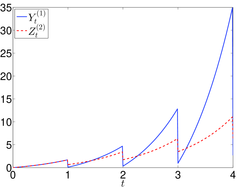
(a) $A\left(t\right)=e^{t}-1$, $\rho_{1}=0.95$, $\rho_{2}=0.5$

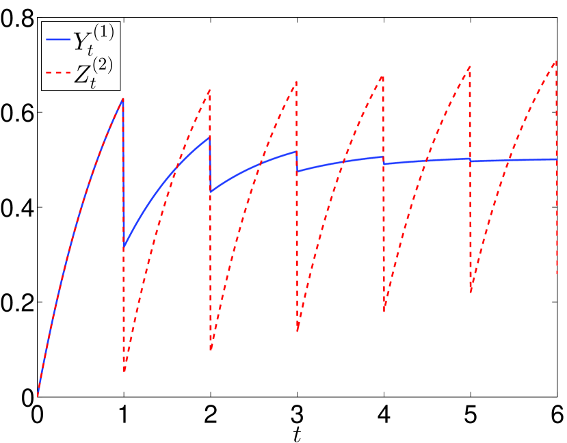
(b) $A\left(t\right)=1-e^{-t}$, $\rho_{1}=0.5$, $\rho_{2}=0.95$

Figure 1: Expectations of $Y_{t}^{(1)}$ and $Z_{t}^{(2)}$ with $b=1$, $T=1$

Proposition 4.

Let us consider the two following assertions:

$$Var\left(Z_{t}^{(2)}\right) \geq Var\left(Y_{t}^{(1)}\right)\text{ for all }t,T>0$$ (18)

$$\text{and }A\left((1-\rho_{2})t\right) \geq (1-\rho_{1})^{2}A(t)\text{ for all }t>0.$$ (19)

Then:

1. Assertion $(\ref{V1})$ implies assertion $(\ref{V2})$.

2. If $A(\cdot)$ is concave, then the converse is also true (namely $\left(\ref{V2}\right)\Longrightarrow\left(\ref{V1}\right)$).

3. As a special case, if $A(\cdot)$ is concave and $1-\rho_{2}\geq\left(1-\rho_{1}\right)^{2}$, then $\left(\ref{V1}\right)$ is true.

All the previous results are valid with reversed inequalities, and concave substituted by convex.

Proof.

Based on $\left(\ref{EYt}\right)$ and $\left(\ref{EZt}\right)$, inequality $\left(\ref{V1}\right)$ is equivalent to

$$A(t-\rho_{2}nT)\geq A(t)-\rho_{1}\left(2-\rho_{1}\right)A(nT)$$ (20)

for all $T>0$, all $n\in\mathbb{N}$, all $nT\leq t<\left(n+1\right)T$. Considering $t=nT$, it implies $\left(\ref{V2}\right)$, so that point one is true.

Now assume $A(\cdot)$ to be concave. Based on $\left(\ref{eq1}\right)$, we have:

$$A(t-\rho_{2}nT)-A(t)+\rho_{1}(2-\rho_{1})A(nT)\geq A((1-\rho_{2})nT)-\left(1-\rho_{1}\right)^{2}A(nT).$$

If $\left(\ref{V2}\right)$ is true, then $\left(\ref{V3}\right)$ is consequently true and $\left(\ref{V1}\right)$ too. This shows the second point.

In the specific case where $A(\cdot)$ is concave and $(1-\rho_{2})\geq\left(1-\rho_{1}\right)^{2}$, we have

$$A((1-\rho_{2})nT)\geq(1-\rho_{2})A(nT)\geq(1-\rho_{1})^{2}A(nT)$$

(based on $\left(\ref{eq2}\right)$ for the first inequality). Hence $\left(\ref{V3}\right)$ is true, so that $\left(\ref{V1}\right)$ is true too. This provides point three.

The reasoning is similar for reversed inequalities and it is omitted. ∎

Example 2.

We now consider the same data as for Example 1, where neither condition $\left(\ref{V2}\right)$ nor the reversed inequality is true on the whole real line. The corresponding variances are plotted in Figures 2(a) (first case) and 2(b) (second case). We can see that the respective variances of $Y_{t}^{(1)}$ and $Z_{t}^{(2)}$ are not ordered in the same way on the whole real line.

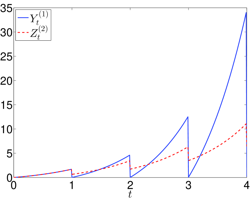
(a) $A\left(t\right)=e^{t}-1$, $\rho_{1}=0.95$, $\rho_{2}=0.5$

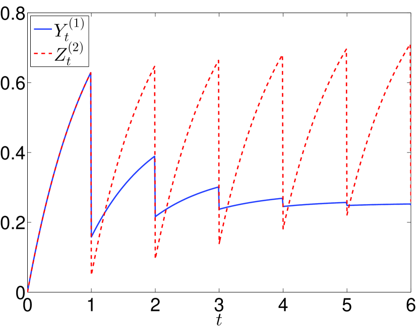
(b) $A\left(t\right)=1-e^{-t}$, $\rho_{1}=0.5$, $\rho_{2}=0.95$

Figure 2: Variances of $Y_{t}^{(1)}$ and $Z_{t}^{(2)}$ with $b=1$, $T=1$

Finally, we easily derive from Propositions 3 and 4 the following corollary, where the expectation and variance of the two processes are compared assuming a power law shape function for the gamma process.

Corollary 1.

We consider $A(t)=\alpha t^{\beta}$ with $\alpha,\beta>0$. Then we get

1. If $\beta\leq(\geq)1$, then

   $$\mathbb{E}\left(Z_{t}^{(2)}\right)\geq\left(\leq\right)\mathbb{E}\left(Y_{t}^{(1)}\right)\forall t\Leftrightarrow(1-\rho_{2})^{\beta}\geq\nolinebreak\left(\leq\right)\left(1\nolinebreak-\nolinebreak\rho_{1}\right).$$

2. If $\beta\leq(\geq)1$, then

   $$Var\left(Z_{t}^{(2)}\right)\geq(\leq)Var\left(Y_{t}^{(1)}\right)\,\forall t\Leftrightarrow(1-\rho_{2})^{\beta}\geq\nolinebreak\left(\leq\right)\left(1-\rho_{1}\right)^{2}.$$

5 Stochastic comparison between $Y_{t}^{(1)}$ and $Z_{t}^{(2)}$

We now come to the stochastic comparison between $Y_{t}^{(1)}$ and $Z_{t}^{(2)}$, as given by (4) and (9), with $\rho$ substituted by $\rho_{i},i=1,2$, respectively.

Proposition 5.

If

$$A\left((1-\rho_{2})nT\right)\geq\left(\leq\right)(1-\rho_{1})A(nT),$$ (21)

then $Y_{nT}^{(1)}\prec_{icx}\left(\succ_{icv}\right)Z_{nT}^{(2)}$.

Proof.

From (5) and (10), we know that $Y_{nT}^{(1)}$ and $Z_{nT}^{(2)}$ are gamma distributed, with distributions $\Gamma\left(A\left(nT\right),\frac{b}{1-\rho_{1}}\right)$ and $\Gamma(A\left((1-\rho_{2})nT\right),b)$, respectively. The results can hence be obtained by application of Lemma 1. ∎

We next focus on the comparison between $Y_{t}^{(1)}-Y_{nT}^{(1)}$ and $Z_{t}^{(2)}-Z_{nT}^{(2)}$.

Proposition 6.

If $A\left(t\right)$ is convex (concave), then for all $nT\leq t<\left(n+1\right)T$:

• $Z_{t}^{(2)}-Z_{nT}^{(2)}\prec_{lr}\left(\succ_{lr}\right)Y_{t}^{(1)}-Y_{nT}^{(1)},$

• $Y_{t}^{(1)}-Y_{nT}^{(1)}\prec_{lc}\left(\succ_{lc}\right)Z_{t}^{(2)}-Z_{nT}^{(2)}.$

Proof.

For $nt\leq t<\left(n+1\right)T$, let us set

$$Y=Y_{t}^{(1)}-Y_{nT}^{(1)}=X_{t}^{\left(n+1\right)}-X_{nT}^{\left(n+1\right)}$$

(see (4)) and

$$Z=Z_{t}^{(2)}-Z_{nT}^{(2)}=X_{t-\rho_{2}nT}^{\left(n+1\right)}-X_{\left(1-\rho_{2}\right)nT}^{\left(n+1\right)}$$

(see (9)). Then $Y$ and $Z$ are gamma distributed, with distributions $\Gamma(A(t)-A(nT))$ and $\Gamma(A\left(t-\rho_{2}nT\right)-A\left(\left(1-\rho_{2}\right)nT\right))$, respectively. Now, the likelihood ratio comparison result is a direct consequence of Lemma 1, because the convexity (concavity) of $A(\cdot)$ entails that

$$A(t)-A(nT)\geq(\leq)A\left(t-\rho_{2}nT\right)-A\left(\left(1-\rho_{2}\right)nT\right).$$

As for the log-concave order, using the notations of Definition 2, we have

$$\left(\log\left(\frac{f_{Y}}{f_{Z}}\right)\right)^{\prime}\left(y\right)=\frac{\left[A\left(t\right)-A\left(nT\right)\right]-\left[A\left(t-\rho_{2}nT\right)-A\left(\left(1-\rho_{2}\right)nT\right)\right]}{y}.$$

This function decreases (increases) when $A\left(t\right)$ is convex (concave), which provides the result. ∎

Hence, if $A\left(t\right)$ is convex (concave), the increment between times $nT$ and $t$ (with $nT\leq t<\left(n+1\right)T$) is smaller (larger) for the ARA1 model than for the ARD1 model in the sense of the likelihood ratio order (and consequently also for the usual stochastic and increasing convex/concave orders), but it has a larger (smaller) variability for the ARA1 model than for the ARD1 model in the sense of the log-concave order.

Based on the previous results, if $A\left(\cdot\right)$ is concave, we have $Z^{(2)}_{t}-Z^{(2)}_{nT}\prec_{lc}Y_{t}^{(1)}-Y_{nT}^{(1)}$ but $Y^{(1)}_{nT}\prec_{lc}Z^{(2)}_{nT}$ (for $nT\leq t<\left(n+1\right)T$). There consequently is no real hope that $Y^{(1)}_{t}\prec_{lc}Z^{(2)}_{t}$. When $A\left(\cdot\right)$ is convex, we have both $Y^{(1)}_{t}-Y^{(1)}_{nT}\prec_{lc}Z^{(2)}_{t}-Z^{(2)}_{nT}$ and $Y^{(1)}_{nT}\prec_{lc}Z^{(2)}_{nT}$, and $Y^{(1)}_{t}\prec_{lc}Z^{(2)}_{t}$ might be valid. However, remembering that the log-concave order is not closed under convolution, see Whitt (1985), the question deserves to be further studied, which is done in the following example.

Example 3.

The function $\log\left(f_{Y^{(1)}_{t}}/f_{Z^{(2)}_{t}}\right)$ is plotted in Figures 3(a) and 3(b) for $\rho_{1}=0.5$, $\rho_{2}=0.4$, $T=1$, $A\left(t\right)=t^{\alpha}$, $n=10$, $b=1$ at time $t=10.2$, with $\alpha=0.75$ and $\alpha=1.25$, respectively. We observe that we do not have $Y^{(1)}_{t}\prec_{lc}Z^{(2)}_{t}$ neither for $\alpha=0.75$ (as expected) nor for $\alpha=1.25$ for which the question was open. As a conclusion, in a general setting, $Y^{(1)}_{t}$ and $Z^{(2)}_{t}$ are not comparable with respect to the log-concave order.

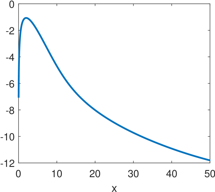
(a) $log(f_{Y_{t}^{(1)}}/f_{Z_{t}^{(2)}})$ for $\alpha=0.75$

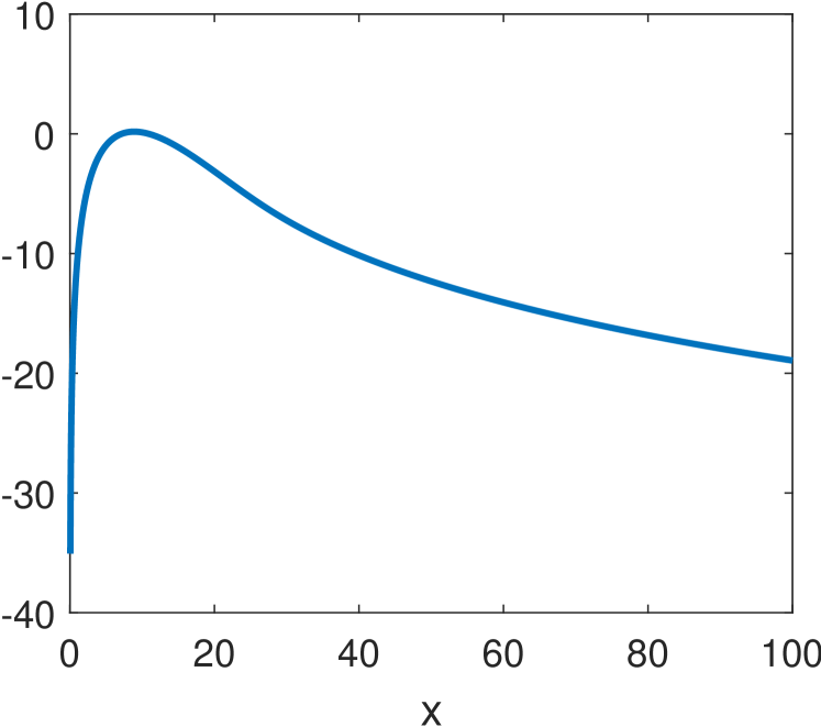
(b) $log(f_{Y_{t}^{(1)}}/f_{Z_{t}^{(2)}})$ for $\alpha=1.25$

Figure 3: Plots of $log(f_{Y_{t}^{(1)}}/f_{Z_{t}^{(2)}})$ for $A(t)=t^{\alpha}$

Next result provides some conditions under which $Y_{t}^{(1)}$ and $Z_{t}^{(2)}$ are comparable with respect to either the increasing convex or concave order.

Theorem 1.

If $A\left(\cdot\right)$ is concave and

$$A\left((1-\rho_{2})t\right)\geq(1-\rho_{1})A(t)\text{ for all }t>0$$ (22)

(condition of Proposition 3, known to be true if $\rho_{1}\geq\rho_{2}$), then $Y_{t}^{(1)}\prec_{icx}Z_{t}^{(2)}$ for all $t\geq 0$ (and all $T\geq 0$).

If $A\left(t\right)$ is convex with a reversed inequality in $\left(\ref{eqA3}\right)$, then $Z_{t}^{(2)}\prec_{icv}Y_{t}^{(1)}$ for all $t\geq 0$ (and all $T\geq 0$).

Proof.

Writing $Y_{t}^{\left(1\right)}=\left(Y_{t}^{\left(1\right)}-Y_{nT}^{\left(1\right)}\right)+Y_{nT}^{\left(1\right)}$ (the same for $Z_{t}^{\left(2\right)}$), the results are direct consequences from Propositions 5 and 6, based on the fact that both increasing convex and concave orders are stable under convolution (Shaked and Shanthikumar, 2007, Thm 4.A.8 (d) page 186). ∎

Example 4 (Increasing convex order).

We consider $t=10.5$, $T=1$, $b=1$, $\rho_{1}$ = $\rho_{2}$= $0.75$ with $A(t)=t^{0.7}$ as a first case (concave case with condition $(\ref{eqA3})$ fulfilled) and $A(t)=t^{1.1}$ as a second case (convex case with reversed condition $(\ref{eqA3})$ fulfilled). The difference

$$\int_{x}^{+\infty}\bar{F}_{Z_{t}^{(2)}}\left(u\right)\leavevmode\nobreak\ du-\int_{x}^{+\infty}\bar{F}_{Y_{t}^{(1)}}\left(u\right)\leavevmode\nobreak\ du$$

is plotted in Figures 4(a) (first case) and 4(b) (second case). As expected, the difference remains positive in the first case, which means that $Y_{t}^{(1)}\prec_{icx}Z_{t}^{(2)}$ (see (1)). We observe that it changes sign in the convex case, which shows that $Z_{t}^{(2)}$ and $Y_{t}^{(1)}$ are not comparable with respect to the increasing convex order.

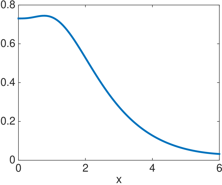
(a) $A(t)=t^{0.7}$

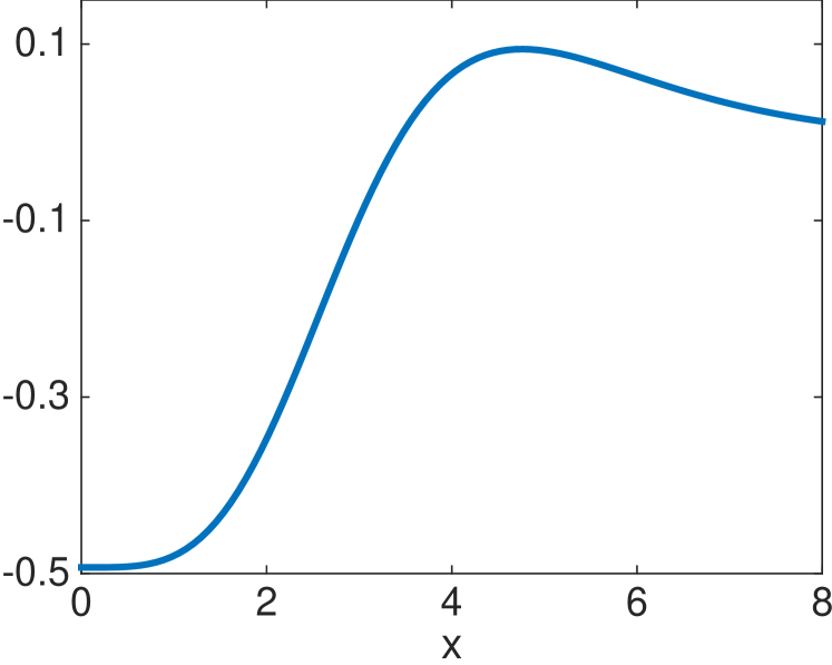
(b) $A(t)=t^{1.1}$

Figure 4: Plots of $\int_{x}^{\infty}\bar{F}_{Z_{t}^{(2)}}(u)du-\int_{x}^{\infty}\bar{F}_{Y_{t}^{(1)}}(u)du$ for $A(t)=t^{\alpha}$

Example 5 (Increasing concave order).

We consider $t=10.5$, $T=1$, $\rho_{1}=0.8$, $\rho_{2}=0.78$, $b=1$ with $A(t)=t^{0.9}$ (concave case with condition $(\ref{eqA3})$ fulfilled) and $A(t)=t^{1.1}$ (convex case with reversed condition $(\ref{eqA3})$ true). The difference $\int_{0}^{x}F_{Z_{t}^{(2)}}(u)du-\int_{0}^{x}F_{Y_{t}^{(1)}}(u)du$ is plotted in Figures 5(a) (first case) and 5(b) (second case). We observe that, as expected, $Z_{t}^{(2)}\prec_{icv}Y_{t}^{(1)}$ (see (2)) in the second case whereas $Z_{t}^{(2)}$ and $Y_{t}^{(1)}$ are not comparable with respect to the increasing concave order in the first case.

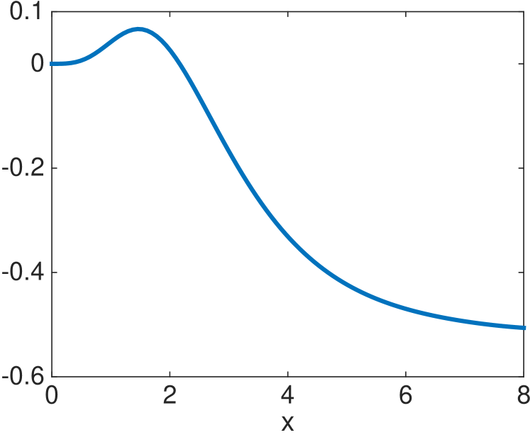
(a) $A(t)=t^{0.9}$

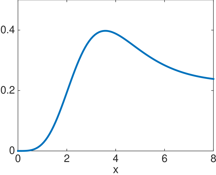
(b) $A(t)=t^{1.1}$

Figure 5: Plots of $\int_{0}^{x}F_{Z_{t}^{(2)}}(u)du-\int_{0}^{x}F_{Y_{t}^{(1)}}(u)du$ for $A(t)=t^{\alpha}$

Finally, we end this section by considering the case of a homogeneous gamma process ($A(t)=at$).

Corollary 2.

Assume that $A(t)=at$ for all $t\geq 0$, where $a>0$. We have the following results:

1. If $\rho_{1}\geq\rho_{2}$, then $Y_{t}^{(1)}\prec_{icx}Z_{t}^{(2)}$ and hence $\mathbb{E}(Y_{t}^{(1)})\leq\mathbb{E}(Z_{t}^{(2)})$ for all $t\geq 0$;

2. If $\rho_{1}\leq\rho_{2}$, then $Z_{t}^{(2)}\prec_{icv}Y_{t}^{(1)}$ and hence $\mathbb{E}(Z_{t}^{(2)})\leq\mathbb{E}(Y_{t}^{(1)})$ for all $t\geq 0$;

3. If $\rho_{1}=\rho_{2}$, then $Y_{t}^{(1)}\prec_{cx}Z_{t}^{(2)}$ and $Z_{t}^{(2)}\prec_{cv}Y_{t}^{(1)}$ and hence $\mathbb{E}(Z_{t}^{(2)})=\mathbb{E}(Y_{t}^{(1)})$ for all $t\geq 0$;

4. $Var\left(Z_{t}^{(2)}\right)\geq Var\left(Y_{t}^{(1)}\right)$ for all $t>0$ if and only if $1-\rho_{2}\geq(1-\rho_{1})^{2}$.

Proof.

Points 1, 2 and 4 are direct consequences of Theorem 1 and Corollary 1. As for point 3, assume that $\rho_{1}=\rho_{2}$. This entails that $\mathbb{E}\left(Y_{t}^{(1)}\right)=\mathbb{E}\left(Z_{t}^{(2)}\right)$. Based on the first two points, the result follows from (Shaked and Shanthikumar, 2007, Theorem 4.A.35 page 197). ∎

6 Mostly equivalent imperfect repair models

In an applied context, parameters $\rho_{1}$ and $\rho_{2}$ for ARD1 and ARA1 models, respectively, will be estimated from feedback data, which will be typically gathered at maintenance times $iT$, $i\geq 1$. As a consequence, we can expect that the estimated parameters $\hat{\rho}_{1}$ and $\hat{\rho}_{2}$ should be such that the corresponding expected deterioration levels should be very similar at maintenance times, namely such that

$$\mathbb{E}\left(Y_{iT}^{\left(1\right)}\right)=\frac{\left(1-\hat{\rho}_{1}\right)A\left(iT\right)}{b}\simeq\mathbb{E}\left(Z_{iT}^{\left(2\right)}\right)=\frac{A\left(\left(1-\hat{\rho}_{2}\right)iT\right)}{b}.$$

There hence is a specific interest for the applications to compare the ARD1 and ARA1 models under the condition

$$\left(1-\rho_{1}\right)A\left(iT\right)=A\left(\left(1-\rho_{2}\right)iT\right)\text{ for }i\geq 1,$$ (23)

on $(\rho_{1},\rho_{2})$, which will lead to mostly equivalent deterioration levels (at least at maintenance times). However, the previous requirement $\left(\ref{req}\right)$ does not seem to have a solution for a general shape function $A\left(\cdot\right)$. We hence restrict the study to the power law case $A\left(t\right)=\alpha t^{\beta}$ (with $\alpha,\beta>0$), for which $\left(\ref{req}\right)$ is just equivalent to

$$1-\rho_{1}=\left(1-\rho_{2}\right)^{\beta}.$$ (24)

This section is hence devoted to this specific power law case with the previous relationship between $\rho_{1}$ and $\rho_{2}$, which ensures that

$$\mathbb{E}\left(Y_{iT}^{\left(1\right)}\right)=\mathbb{E}\left(Z_{iT}^{\left(2\right)}\right)\text{ for all }i\geq 1.$$

Remark 6.

This specific “equivalent” case has a similar spirit to that detailed in (Doyen and Gaudoin, 2004, Property 4), where the authors match the minimal wear intensities of two imperfect repair models for recurrent events, based on the reduction of either virtual age or failure intensity.

In case of a homogeneous gamma process ($\beta=1$), the equivalent case corresponds to identical repair efficiencies for both ARD1 and ARA1 models ($\rho_{1}=\rho_{2}$), which has already been studied in Corollary 2 (point 3). We now investigate the case of a general $\beta$.

In the equivalent case, there is equality in $\left(\ref{eqA1}\right)$, $\left(\ref{eqA2}\right)$ and $\left(\ref{eqA3}\right)$. Based on the fact that $A\left(\cdot\right)$ is concave (convex) when $\beta\leq\left(\geq\right)1$, we directly get the following results from Proposition 5, Theorem 1 and Corollary 1.

Corollary 3.

Assume that $A\left(t\right)=\alpha t^{\beta}$ (with $\alpha,\beta>0$) and that $(\rho_{1},\rho_{2})$ fulfills $\left(\ref{Eq rho 1 rho2}\right)$ (equivalent case). Then:

1. $Z_{nT}^{(2)}\prec_{cv}Y_{nT}^{(1)}$ and $Y_{nT}^{(1)}\prec_{cx}Z_{nT}^{(2)}$ (which both entail that $var\left(Z_{nT}^{\left(2\right)}\right)\geq var\left(Y_{nT}^{\left(1\right)}\right)$, see (Shaked and Shanthikumar, 2007, (3.A.4) page 110)) for all $n\geq 1$.

2. If $\beta\leq\left(\geq\right)1$, then $Y_{t}^{(1)}\prec_{icx}\left(\succ_{icv}\right)Z_{t}^{(2)}$ (which entails that $\mathbb{E}\left(Y_{t}^{\left(1\right)}\right)\leq\left(\geq\right)\mathbb{E}\left(Z_{t}^{\left(2\right)}\right)$) for all $t\geq 0$.

3. If $\beta\leq 1$, then $Var\left(Z_{t}^{(2)}\right)\geq Var\left(Y_{t}^{(1)}\right)$ for all $t\geq 0$.

Remark 7.

Based on the previous result, we can see that even if the two imperfect repair models provide similar expected deterioration levels at maintenance times, there are differences in both their location and spread between the repairs. For instance, considering $\beta\leq 1$, a possible by-product of $Y_{t}^{(1)}\prec_{icx}Z_{t}^{(2)}$ is that $\mathbb{E}((Y_{t}^{(1)}-h)^{+})\leq\mathbb{E}((Z_{t}^{(2)}-h)^{+})$ for any $h>0$, see, e.g., (Shaked and Shanthikumar, 2007, (4) p 182). If $h$ is a critical deterioration level in an application context, $(Y_{t}^{(1)}-h)^{+}$ and $(Z_{t}^{(2)}-h)^{+}$ correspond to the hazardous part of deterioration (beyond the critical level) and this means that the expected “risk” is lower for the ARD1 model than for the ARA1 one.

Note that Corollary 3 does not provide any insight for the comparison of the variances at time $t$ when $\beta>1$, which hence deserves a different analysis on which we now focus.

Proposition 7.

Let $\beta>1$ and let

$$g\left(x\right)=x^{\beta}-\left(x-\rho_{2}\right)^{\beta}-\left(1-(1-\rho_{2})^{2\beta}\right)$$ (25)

for $x\in[1,2)$.

• If $g\left(2^{-}\right)\leq 0$, then

  $$Var\left(Y_{t}^{(1)}\right)\leq Var\left(Z_{t}^{(2)}\right)$$ (26)

  for all $t\geq 0$.

• If $g\left(2^{-}\right)>0$, there exists one single $x^{\ast}\in(1,2)$ such that $g\left(x^{\ast}\right)=0$. Also:

  • Inequality $\left(\ref{Ineq VAR}\right)$ is true for all $t\geq t^{\ast}=\left\lceil\frac{1}{x^{\ast}-1}\right\rceil T$, where $\left\lceil\cdot\right\rceil$ stands for the ceiling function;

  • For each $n<\frac{1}{x^{\ast}-1}$, inequality $\left(\ref{Ineq VAR}\right)$ is true for all $t\in[nT,x^{\ast}nT)$, with a reversed inequality for $t\in[x^{\ast}nT,\left(n+1\right)T)$.

Proof.

For $nT\leq t<(n+1)T$, it is easy to check that $\left(\ref{Ineq VAR}\right)$ is equivalent to

$$t^{\beta}-\left(1-(1-\rho_{2})^{2\beta}\right)(nT)^{\beta}\leq\left(t-\rho_{2}nT\right)^{\beta},$$

which can also be written as $g\left(\frac{t}{nT}\right)\leq 0$ where $1\leq\frac{t}{nT}\leq 1+\frac{1}{n}$ and where $g$ is defined by $\left(\ref{g}\right)$ for $x\in\bigcup_{n\geq 1}[1,1+\frac{1}{n})=[1,2)$.

As $\beta>1$, the function $g$ increases from $g\left(1\right)$ to $g\left(2^{-}\right)$ and based on the fact that $var\left(Z_{nT}^{\left(2\right)}\right)\geq var\left(Y_{nT}^{\left(1\right)}\right)$ (first point of Corollary 3), we have $g\left(1\right)\leq 0$. As for the sign of

$$g\left(2^{-}\right)=2^{\beta}-\left(2-\rho_{2}\right)^{\beta}-\left(1-(1-\rho_{2})^{2\beta}\right),$$

there are two possibilities, which lead to the following cases:

• If $g\left(2^{-}\right)\leq 0$, then $g\left(x\right)\leq 0$ for all $x\in[1,2)$ and $\left(\ref{Ineq VAR}\right)$ is true for all $t\geq 0$.

• If $g\left(2^{-}\right)>0$, there exists one single $x^{\ast}\in(1,2)$ such that $g\left(x^{\ast}\right)=0$, with $g\left(x\right)<0$ for all $x\in[1,x^{\ast})$ and $g\left(x\right)>0$ for all $x\in(x^{\ast},2)$.

  • If $1+\frac{1}{n}\leq x^{\ast}$ (namely $n\geq\frac{1}{x^{\ast}-1}$), then $g\left(x\right)<0$ for all $x\in[1,1+\frac{1}{n})$ and $\left(\ref{Ineq VAR}\right)$ is true for all $t\in[nT,\left(n+1\right)T)$. This inequality is hence true for all $t\geq n^{\ast}T$ with $n^{\ast}=\left\lceil\frac{1}{x^{\ast}-1}\right\rceil$.

  • If $1+\frac{1}{n}>x^{\ast}$ (namely $n<\frac{1}{x^{\ast}-1}$), then $g\left(x\right)<0$ for all $x\in[1,x^{\ast})$ and $\left(\ref{Ineq VAR}\right)$ is true for all $t\in[nT,x^{\ast}nT)$, with a reversed inequality for $t\in[x^{\ast}nT,\left(n+1\right)T)$.

∎

Remark 8.

In the case where $g\left(2^{-}\right)>0$, note that the inequality $n<\frac{1}{x^{\ast}-1}$ is always valid for $n=1$ so that for small $n$, the difference $Var\left(Y_{t}^{(1)}\right)-Var\left(Z_{t}^{(2)}\right)$ will always cross 0 (from - to +) on $[nT,\left(n+1\right)T)$ (and will remain negative for larger $n$).

7 Maintenance strategies

7.1 The reward function

This section is devoted to the analysis of maintenance strategies considering the two types of repair. In all the section, the system is assumed to provide a reward which decreases when the deterioration level of the system increases. Based on classical functions used in the insurance literature (Rolski et al. (1998)), we assume that the reward function is given by

$$g(x)=\left(b_{1}-k_{1}e^{\alpha_{1}x}\right)\mathbf{1}_{\left\{0\leq x\leq c\right\}}+\left(b_{2}-k_{2}e^{\alpha_{2}x}\right)\mathbf{1}_{\left\{c<x\right\}},$$ (27)

with $b_{1},b_{2},\alpha_{1},\alpha_{2},k_{1},k_{2},c>0$ and $x\geq 0$, where $g(x)$ stands for the unitary reward per unit time when the degradation level of the system is $x$. The function $g$ is supposed to be continuous and positive on $[0,c)$, which implies that

$$b_{2}-k_{2}e^{\alpha_{2}c}=b_{1}-k_{1}e^{\alpha_{1}c}>0.$$ (28)

Also, we assume that $\alpha_{1}\leq\alpha_{2}$ and $k_{1}\leq k_{2}$ so that level $c$ appears as a critical level, from which the system becomes less performing.

With the previous assumptions, it is easy to check that $g$ is a concave function and that $g(x)>0$ if and only if $x<L=\frac{\ln(b_{2}/k_{2})}{\alpha_{2}}$. Level $L$ hence appears as a critical threshold.

An example of reward function is plotted in Figure 6 with parameters $\alpha_{1}=0.1$, $b_{1}=11$ monetary units per time unit (m.t.u.), $\alpha_{2}=0.25$, $k_{1}=1$ m.t.u., $k_{2}=1$ m.t.u., $c=4$ time units (t.u.), and $b_{2}$ is obtained through (28). With this dataset $L\simeq 10.0144$.

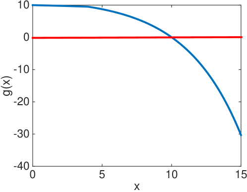
Figure 6: Reward function for $\alpha_{1}=0.1$, $b_{1}=11$, $\alpha_{2}=0.25$, $k_{1}=1$, $k_{2}=1$, $c=4$

Two different maintenance strategies are envisioned in the two following subsections. In each case, the system is put into operation at time $t=0$ and it degrades according to a non-homogeneous gamma process with parameters $A(t)$ and $\beta$. For each maintenance strategy, the two imperfect repair models are envisioned (ARA1 or ARD1) and the comparison between the two types of repair is performed through their corresponding expected reward (profit) rates per unit time on a long time run.

7.2 $(n,T)$ policy

Starting from $n\in\mathbb{N}^{*}$ and $T>0$, the $(n,T)$ maintenance scheme is developed as follows:

• Imperfect repairs based on either one of the two models (ARD1 or ARA1) are performed at times $T,2T,3T,\ldots$

• Each imperfect repair costs $C_{r}$ monetary units (m.u.),

• The profit per unit time is given by the reward function $g$ from (27),

• The system is replaced by a new one at the time of the $n$-th imperfect repair ($nT$) with a cost of $C$ m.u..

Based on the renewal reward theorem, see, e.g., Tijms (2003), the long time reward rate per unit time for this policy is given by:

$$R_{ARD}(n,T)=\frac{\int_{0}^{nT}\mathbb{E}\left(g(Y_{s}^{(1)})\right)ds-(n-1)C_{r}-C}{nT}$$ (29)

when ARD1 repairs are considered and

$$R_{ARA}(n,T)=\frac{\int_{0}^{nT}\mathbb{E}\left(g(Z_{s}^{(2)})\right)ds-(n-1)C_{r}-C}{nT}$$ (30)

for ARA1 repairs, where $Y_{s}^{(1)}$ and $Z_{s}^{(2)}$ are is given by (4) and (9), respectively, with $\rho$ substituted by $\rho_{i},i=1,2$ .

Remark 9.

Based on the fact that the function $-g(\cdot)$ is increasing and convex, the previously obtained theoretical results allow to derive several observations on the reward rates:

• From Propositions 1 and 2, we get that $\mathbb{E}\left(-g(Y_{t}^{(1)})\right)$ and $\mathbb{E}\left(-g(Z_{t}^{(2)})\right)$ decrease with $\rho_{1}$ and $\rho_{2}$ for all $t>0$, respectively. This entails that the objective profit rates $R_{ARD}(n,T)$ and $R_{ARA}(n,T)$ increase with the effectiveness of the repair ($\rho_{1}$ and $\rho_{2}$, respectively) for both ARD1 and ARA1 models.

• If the shape function $A(\cdot)$ is concave and $A((1-\rho_{2})t)\geq(1-\rho_{1})A(t)$ for all $t>0$ (Condition $(\ref{eqA3})$), then Theorem 1 entails that

  $$\mathbb{E}\left(g(Z_{t}^{(2)})\right)\leq\mathbb{E}\left(g(Y_{t}^{(1)})\right),\quad\forall t>0,$$

  from which we derive that the objective profit functions for the two repair models are comparable:

  $$R_{ARA}\left(n,T\right)\leq R_{ARD}\left(n,T\right)\text{ for all }n,T.$$

We now come to some numerical illustrations.

Example 6.

The parameters of the gamma process are $A(t)=t^{0.5}+t^{0.75}$ (concave function) and $b=1$; those for the reward reward function $g$ are $\alpha_{1}=0.1$, $\alpha_{2}=0.25$, $k_{1}=1$, $k_{2}=1$, $b_{1}=11$, $c=4$, which implies that $b_{2}=12.2265$. The $(n,T)$ policy is considered with $C_{r}=2$ m.u. as cost of imperfect repair and $C=25$ m.u. as replacement cost.

Figure 7 shows the operating profit rate given in (29) for both ARD1 and ARA1 models using $\rho_{1}=\rho_{2}=0.5$ (for which inequality $(\ref{eqA3})$ is true). The computations have been made using 8 points for $T$ from 1 to 6 and 10 points for $n$ from 1 to 10 with 5000 simulations in each point. The Simpson method is applied for the integrals in (29), with 20 points from $0$ to $nT$.

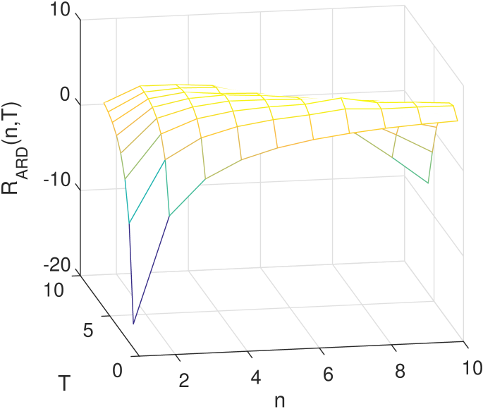
(a) ARD1 model

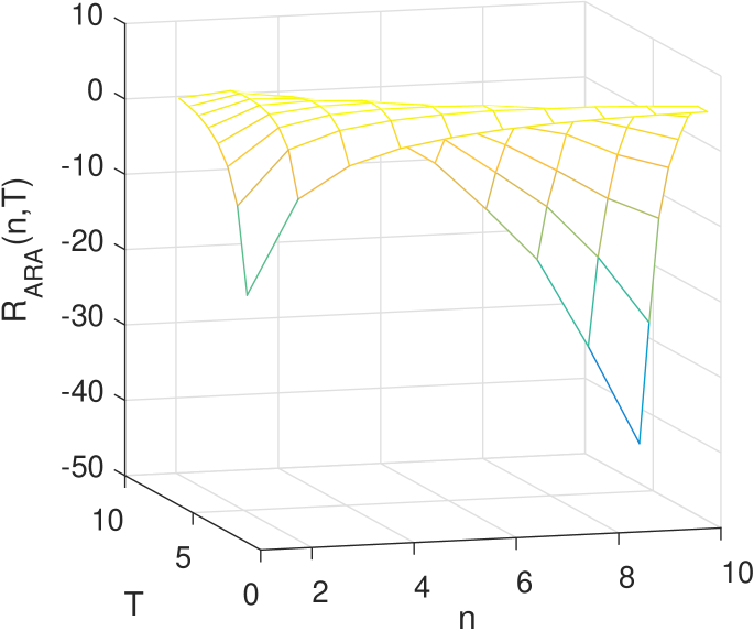
(b) ARA1 model

Figure 7: Operational profit rate, $(n,T)$ policy

Under an ARD1 model, the optimal profit rate is obtained for $(n,T)=(7,2.43)$ with a profit rate of $R_{ARD}(7,2.43)=6.85$ m.u. per unit time. Under an ARA1 model, the optimal profit rate is obtained for $(n,T)=(4,3.14)$ with a profit rate of $R_{ARA}(4,3.14)=5.29$ m.u. per unit time. Figure 8(a) shows the difference of the profit rates under the two repair models, that is, $R_{ARD}(n,T)-R_{ARA}(n,T)$ for all $n$ and $T$. As expected from the previous theoretical results, $R_{ARA}(n,T)\leq R_{ARD}(n,T)$. Also, we can observe that the difference between the two rates increases as $n$ and $T$ increases.

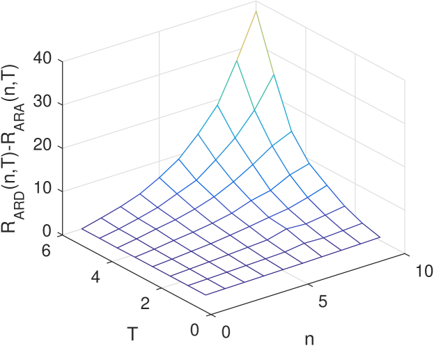
(a) Case $\rho_{1}=\rho_{2}=0.5$

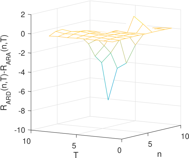
(b) Case $\rho_{1}=0.31$ and $\rho_{2}=0.5$

Figure 8: Differences between the operational profit rates, $(n,T)$ policy

Example 7.

Keeping the same parameters as in the previous example except from the repair efficiency for the ARD1 model which becomes $\rho_{1}=0.31$, Figure 8(b) shows the difference between the profit rates under the two repair models. Here $A(t)=t^{0.5}+t^{0.75}$ is concave but condition (22) of Theorem 1 is not valid any more. We observe that there is no dominance of the profit rate of one model over the other.

Although the $(n,T)$ policy allows us to compare the two models of repair, under this maintenance policy, the system is (imperfectly) repaired even when the system is so degraded that the reward has become negative. We now suggest a more realistic condition-based maintenance strategy, where the maintenance action depends on the degradation level of the system.

7.3 (M,T) policy

Let $T>0$ and let $M\in[0,L)$ be a preventive maintenance threshold. (We recall that $L$ is the critical threshold defined in Subsection 7.1 from where the reward becomes negative). The $(M,T)$ condition-based maintenance scheme is developed as follows:

• The system is inspected at times $T,2T,3T,\ldots$ and the system degradation level is checked.

• By an inspection:

  • If the degradation level does not exceed the threshold $M$, an imperfect repair based on either one of the two models (ARD1 or ARA1) is performed with a cost of $C_{r}$ m.u.;

  • If the degradation level is between levels $M$ and $L$, a preventive replacement is performed and the system is instantaneously replaced by a new one with a cost of $C_{p}$ m.u.;

  • If the degradation level exceeds $L$, a instantaneous corrective replacement takes place with a cost of $C_{c}$ m.u..

• The profit per unit time is given by the reward function $g$ from (27).

The successive (corrective or preventive) replacements of the system appear as the points of a renewal process, and the long time profit rate per unit time is given by

$$C_{ARD}(T,M)$$

$$= \frac{\mathbb{E}\left(\int_{0}^{R}g\left(Y_{s}^{(1)}\right)ds-C_{r}\left([R/T]-1\right)-C_{p}\mathbf{1}_{\left\{M\leq Y_{R}^{(1)}<L\right\}}-C_{c}\mathbf{1}_{\left\{L\leq Y_{R}^{(1)}\right\}}\right)}{\mathbb{E}(R)}$$

for the ARD1 model, with a similar expression for the ARA1 model ($C_{ARA}(T,M)$), where $R$ stands for the time to a system replacement and $g$ denotes the reward function given by (6). Due to the complexity of the $(M,T)$ policy, there is no hope here to find analytical conditions that could ensure the dominance of one function $C_{ARD}(T,M)$ or $C_{ARA}(T,M)$ over the other. Their comparison is hence made on a numerical example.

Example 8.

The parameters of the gamma process are $A(t)=1.3t$ and $b=0.8$. For the reward function $g$, they are $\alpha_{1}=0.4$, $\alpha_{2}=0.5$, $b_{1}=800$, $k_{1}=1.05$, $k_{2}=1.07$, $c=8$, which implies $b_{2}=832.6609$ and $L=13.3139$. The repair efficiencies of the ARD1/ARA1 repairs are $\rho_{1}=\rho_{2}=0.9$. Their common cost is $C_{r}=200$ m.u.. The cost of a preventive replacement is $C_{p}=1000$ m.u. whereas it is $C_{c}=1300$ m.u. for a corrective one. Figure 9(a) shows the profit rate for the maintained system under an ARD1 repair. The optimal maintenance strategy is obtained for $(M,T)=(9.21,3.05)$ with a profit rate of $C_{ARD}(3.05,9.21)=673.94$ m.u. per unit time. Figure 9(b) shows the profit rate for the ARA1 repairs. The optimal maintenance strategy is obtained for $(M,T)=(10.24,3.05)$ with a profit rate of $C_{ARA}(3.05,10.24)=684.34$ m.u. per unit time. These figures have been computed considering a grid of 10 points for $T$ from 1.14 to 4 and a grid of 13 points for $M$ from 1 to $L$ and 10000 simulations for each pair of points.

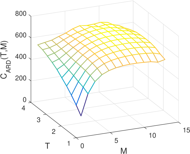
(a) $\rho_{1}=0.9$, ARD1 model

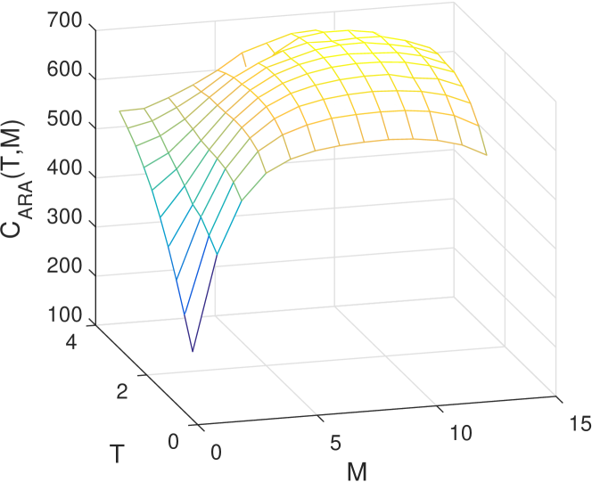
(b) $\rho_{2}=0.9$, ARA1 model

Figure 9: Operational profit rates, $(M,T)$ policy

Figure 10 shows the difference between the profit rates $C_{ARD}(T,M)\leavevmode\nobreak\ -\leavevmode\nobreak\ C_{ARA}(T,M)$ for this dataset. Although conditions of Theorem 1 are fulfilled, we can see that the sign of the difference changes, so that there is no dominance of the profit rate of one model on the other.

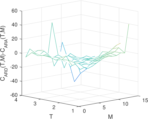
Figure 10: Difference of operational profit rates, $\rho_{1}=\rho_{2}=0.9$

8 Conclusions and perspective

Two imperfect repair models for a degrading system are compared in this paper. The comparison is performed in terms of location and spread of the two resulting stochastic processes. Results are provided in terms of moments and likelihood ratio ordering, as well as in terms of (increasing) convex/concave ordering, which is not so common in the reliability literature. Two maintenance strategies are also developed, which are assessed through a reward function, which takes into account the effective deterioration level of the system (the lower the deterioration level, the higher the reward), contrary to classical objective functions from the literature.

The paper is developed under a periodic imperfect repair scheme, for sake of simplification. It is however easy to check that all the results of the paper would remain valid under a deterministic non periodic repair scheme (with the same maintenance times for both imperfect repair models), with very slight modifications. Even more, considering random maintenance times (independent on the deterioration level and identically distributed for both imperfect repair models), most results would also remain valid, such as the likelihood ratio and (increasing) convex/concave comparison results, based on the closure under mixture property of these stochastic orders (Shaked and Shanthikumar, 2007, Thm 1.C.15. p 48, Thm 4.A.8. p 185).

Note also that if the paper focuses on some specific stochastic orders, other ones could also be considered such as Laplace transform or Excess Wealth orders for instance. Other questions of interest concern the comparison of remaining lifetimes, considering the system as failed (or too degraded) when its deterioration level is beyond a fixed failure (critical) threshold. From a theoretical point of view, this seems a difficult issue in a general setting. One could then look at partial results in specific situations.

Another point of interest would be to try and compare the two types of imperfect repairs dropping the gamma-process assumption. Based on the fact that, under technical conditions, normal random variables are comparable with respect to several stochastic orders (see, e.g., Müller and Stoyan (2002)), one can wonder whether it could be possible to get some similar results as in the paper for Wiener processes with drift. (Not all however, because comparison results between normal random variables in the likelihood ratio ordering sense require that the random variables share the same variance, which cannot be the case in our context. The same for the log-concave order, which requires that the two normal random variables share the same mean, see Whitt (1985)). Other deteriorations processes might also be envisioned, such as inverse Gaussian or inverse Gamma processes.

Finally, other maintenance strategies could be envisioned, based on either one of the two types of imperfect repair.

References

- Alaswad and Xiang (2017) Alaswad, S., Xiang, Y., 2017. A review on condition-based maintenance optimization models for stochastically deteriorating system. Reliability Engineering & System Safety 157, 54–63.
- Barlow and Proschan (1964) Barlow, R., Proschan, F., 1964. Comparison of replacement policies and renewal theory implications. The Annals of Mathematical Statistics 35 (2), 577–589.
- Barlow and Proschan (1965) Barlow, R. E., Proschan, F., 1965. Mathematical theory of reliability. Vol. 17 of Classics in Applied Mathematics. Society for Industrial and Applied Mathematics (SIAM), Philadelphia, PA, with contributions by Larry C. Hunter, 1996.
- Caballé et al. (2015) Caballé, N. C., Castro, I. T., Pérez, C. J., Lanza-Gutiérrez, J. M., 2015. A condition-based maintenance of a dependent degradation-threshold-shock model in a system with multiple degradation processes. Reliability Engineering & System Safety 134, 98–109.
- Castro and Mercier (2016) Castro, I. T., Mercier, S., 2016. Performance measures for a deteriorating system subject to imperfect maintenance and delayed repairs. Proceedings of the Institution of Mechanical Engineers, Part O: Journal of Risk and Reliability 230 (4), 364–377.
- Chen et al. (2015) Chen, N., Ye, Z.-S., Xiang, Y., Zhang, L., 2015. Condition-based maintenance using the inverse gaussian degradation model. European Journal of Operational Research 243 (1), 190–199.
- Denuit and Lefévre (1997) Denuit, M., Lefévre, C., 1997. Some new classes of stochastic order relations among arithmetic random variables, with applications in actuarial sciences. Insurance: Mathematics and Economics 20, 197–213.
- Denuit and Vermandele (1999) Denuit, M., Vermandele, C., 1999. Lorenz and excess wealth orders, with applications in reinsurance theory. Scandinavian Actuarial Journal 1999 (2), 170–185.
- Doyen and Gaudoin (2004) Doyen, L., Gaudoin, O., 2004. Classes of imperfect repair models based on reduction of failure intensity or virtual age. Reliability Engineering & System Safety 84 (1), 45–56.
- Fang and Tang (2014) Fang, L., Tang, W., 2014. On the right spread ordering of series systems with two heterogeneous weibull components. Journal of Inequalities and Applications 2014 (190).
- Giorgio and Pulcini (2018) Giorgio, M., Pulcini, G., 2018. A new state-dependent degradation process and related model misidentification problems. European Journal of Operational Research 267 (3), 1027–1038.
- Hong et al. (2014) Hong, H. P., Zhou, W., Zhang, S., Ye, W., 2014. Optimal condition-based maintenance decisions for systems with dependent stochastic degradation of components. Reliability Engineering & System Safety 121, 276–288.
- Hu et al. (2015) Hu, C.-H., Lee, M.-Y., Tang, J., 2015. Optimum step-stress accelerated degradation test for wiener degradation process under constraints. European Journal of Operational Research 241 (2), 412–4211.
- Huynh et al. (2014) Huynh, K. T., Castro, I. T., Barros, A., Bérenguer, C., 2014. On the use of mean residual life as a condition index for condition-based maintenance decision-making. IEEE Transactions on Systems, Man, and Cybernetics: Systems 44(7), 877–893.
- Khaledi and Shaked (1991) Khaledi, B.-E., Shaked, M., 1991. Ordering conditional lifetimes of coherent systems. Journal of Statistical Planning and Inference 38 (6), 865–876.
- Kijima (1989) Kijima, M., 1989. Some results for repairable systems with general repair. Journal of Applied Probability 26 (1), 89–102.
- Kochar and Xu (2009) Kochar, S., Xu, M., 2009. Comparisons of parallel systems according to the convex transform order. Journal of Applied Probability 46 (2), 342–352.
- Liu et al. (2017) Liu, B., Wu, S., Xie, M., Kuo, W., 2017. A condition-based maintenance policy for degrading systems with age- and state-dependent operating cost. European Journal of Operational Research 263 (3), 879–887.
- Mercier and Castro (2013) Mercier, S., Castro, I., 2013. On the modelling of imperfect repairs for a continuously monitored gamma wear process through age reduction. Journal of Applied Probability 50 (4), 1057–1076.
- Mercier and Pham (2012) Mercier, S., Pham, H., 2012. A preventive maintenance policy for a continuously monitored system with correlated wear indicators. European Journal of Operational Research 222 (2), 263–272.
- Müller and Stoyan (2002) Müller, A., Stoyan, D., 2002. Comparison methods for stochastic models and risks. John Wiley Sons.
- Ohnishi (2002) Ohnishi, M., 2002. Stochastic Models in Reliability and Maintenance, Osaki Edition. Springer, Berlin, Ch. Stochastic orders in reliability theory, pp. 31–63.
- Rolski et al. (1998) Rolski, J., Schmidli, H., Schmidt, V., Teugels, J., 1998. Stochastic Processes for Insurance and Finance. John Wiley & Sons.
- Sadeghi et al. (2018) Sadeghi, J., Najar, M., Mollazadeh, M., Yousefi, B., Zakeri, J., 2018. Improvement of railway ballast maintenance approach, incorporating ballast geometry and fouling conditions. Journal of Applied Geophysics.
- Shaked and Shanthikumar (2007) Shaked, M., Shanthikumar, J. G., 2007. Stochastic Orders. Springer.
- Tijms (2003) Tijms, H., 2003. A First Course in Stochastic Models. John Wiley & Sons.
- Van Noortwijk (2009) Van Noortwijk, J., 2009. A survey of the application of Gamma processes in maintenance. Reliab. Eng. Syst. Saf. 94 (1), 2–21.
- Whitt (1985) Whitt, W., 1985. Uniform conditional variability ordering. Journal of Applied Probability 22 (3), 619–633.
- Zhang et al. (2015) Zhang, M., Gaudoin, O., Xie, M., 2015. Degradation-based maintenance decision using stochastic filtering for systems under imperfect maintenance. European Journal of Operational Research 245, 531–541.