Abstract

This paper develops maintenance policies for a system under condition monitoring. We assume that a number of defects may develop and the degradation process of each defect follows a gamma process, respectively. The system is inspected periodically and maintenance actions are performed on the defects present in the system. The effectiveness of the maintenance is assumed imperfect and it is modelled using a geometric process. By performing these maintenance actions, different costs are incurred depending on the type and the degradation levels of the defects. Furthermore, once a linear combination of the degradation processes exceeds a pre-specified threshold, the system needs a special maintenance and an extra cost is imposed. The system is renewed after several preventive maintenance activities have been performed. The main concern of this paper is to optimise the time between renewals and the number of renewals. Numerical examples are given to illustrate the results derived in the paper.

Keywords: gamma process, geometric process, preventive maintenance, condition-based maintenance, maintenance constraints

1 Introduction

Condition-based maintenance has been extensively studied in the reliability literature due to the emergence of advanced condition monitoring and data collection techniques. Many papers have been published to either model the degradation processes of assets [23], [32], [11],[33] or to optimise maintenance policies [8],[19],[34]. To obtain a comprehensive view of the development in condition-based maintenance, the reader is referred to review papers, see [14],[23],[2], for example.

A number of degradation processes have been considered in condition-based maintenance policies. Many authors investigate different maintenance policies, considering only one degradation process such as the gamma process [8], the Wiener process [25], the inverse Gaussian process [10] and the Ornstein-Uhlenbeck process [11]. Some consider condition-based maintenance policies for assets suffering a number of degradation processes. For example, [7] proposes a condition-based maintenance strategy for a system subject to two dependent causes of failure, degradation and sudden shocks: The internal degradation is reflected by the presence of multiple degradation processes in the system, and degradation processes start at random times following a Non-homogeneous Poisson process and their growths are modelled by using a gamma process. [13] consider maintenance policies monitored by a process of the average of a number of degradation processes.

In this paper, we consider a system on which many different types of defects develops over the time. If a linear combination of the degradation processes exceeds a pre-specified threshold in an inspection time, maintenance is carried out. There are many real-world examples behaving like that in the real world. For example, in the civil engineering, several different types of defects, such as fatigue cracking and pavement deformation, may develop simultaneously on a pavement network. The mechanism of these defects may be different: fatigue cracking is caused by the failure of the surface layer or base due to repeated traffic loading (fatigue), and pavement deformation is the result of weakness in one or more layers of the pavement that has experienced movement after construction [1]. As such, the deteriorating processes of these defects are different in the sense that the parameters in the degradation processes may differ. Furthermore, both the approaches to repairing these defects and the cost of repairing them differ from defect to defect. The time to repair such a system may be the time when a linear combination of those defects exceeds a pre-specified threshold. In the civil engineering literature, for example, [22] propose a linear combination of defects of pavement condition indexes and suggest that a pavement needs maintenance once its combined condition index exceeds a pre-specified threshold. It should also be noted that such deterioration might cause partial loss of system functionality. As such, there is no need to overhaul or renew the entire system unless its combined index exceeds a threshold that is large enough.

Inspired from the above real world example, this paper develops maintenance policies for a system with many degradation processes. The system is inspected periodically. Following an inspection, an imperfect repair is performed. These imperfect repairs are modelled using geometric process. Costs of repairing different defects are different and, if the linear combination of the magnitudes of a set of defects exceeds a pre-specified threshold, an additional cost is incurred. A replacement is carried out once the number of inspections exceeds an optimum value.

The remainder of the paper is structured as follows. Section 2 introduces the notations and assumptions that will be used in the paper. Section 3 derives distributions of hitting time and considers random effects. Section 4 derives maintenance policies and proposes methods of optimisation. Section 5 illustrates the maintenance policies with numerical examples. Section 6 offers discussion on some of the assumptions in this paper. Section 7 concludes the paper.

2 Assumptions

This paper makes the following assumptions.

1. Defects of $n$ types develop through $n$ degradation processes on a system, respectively.

2. The system is inspected every $T$ time units ($T>0$).

3. The system is new at time $t=0$.

4. Two types of maintenance are taken: an imperfect maintenance and a complete replacement of the system. The imperfect maintenance restores the system to a state between a good-as-new state (which is resulted from a replacement) and a bad-as-old state (which is resulted from a minimal repair) and is modelled using a geometric process. The replacement completely renews the system.

5. On performing these maintenance actions, a sequence of costs is incurred. Repairing the $k$-th ($k=1,2,\ldots,n$) defect incurs two types of cost: a fixed cost, and a variable cost that depends on the degradation level of the $k$-th defect. Furthermore, if the linear combination of the magnitudes of a set of defects exceeds a pre-specified threshold, an additional cost is incurred.

6. Imperfect maintenance actions are performed every $T$ time units and preventive replacement is performed at the time of the $N$-th inspection.

7. Maintenance time is so short that it can be neglected.

3 Model development

[26] optimise inspection decisions for scour holes, on the basis of the uncertainties in the process of occurrence of scour holes and, given that a scour hole has occurred, of the process of current-induced scour erosion. The stochastic processes of scour-hole initiation and scour-hole development was regarded as a Poisson process and a gamma process, respectively. [18] construct a tractable gamma-process model incorporating a random effect and fit the model to some data on crack growth. In the following, we make similar assumptions: The stochastic processes of defect initiation and defect development was regarded as a Poisson process and a gamma process, respectively.

3.1 Modelling the occurrences of the defects

Denote the successive times between occurrences of the defects by the infinite sequence of non-negative real-valued random quantities $T_{1},T_{2},...$. Assume the defect initiation follows a homogeneous Poisson process. Similar to the assumptions made in [26], we assume the defect inter-occurrence times are exchangeable and they exhibit the memorylessness property. That is, the order in which the defects occur is irrelevant and the probability distribution of the remaining time until the occurrence of the first defect does not depend on the fact that a defect has not yet occurred since the last replacement. According to [26], the joint probability density function of $T_{1},T_{2},....,T_{n}$ is given by

$$p_{T_{1},T_{2},...,T_{n}}(t_{1},...,t_{n})=\int_{0}^{\infty}\prod_{k=1}^{n}\frac{1}{\lambda}\exp\left(-\frac{t_{k}}{\lambda}\right)p_{\Lambda}(\lambda)d\lambda,$$ (1)

where $(t_{1},t_{2},....,t_{n})\in\mathbb{R}^{n}_{+}$, $p_{\Lambda}(\lambda)=\frac{1}{\Gamma(\nu)}\mu^{\nu}\lambda^{-(\nu+1)}e^{-\nu/\lambda}1_{\{\lambda>0\}}$, where $\mu$ and $\nu$ are parameters that can be estimated from given observations, $1_{\{\lambda>0\}}=1$ if $\lambda>0$ and $1_{\{\lambda>0\}}=0$ otherwise. With the constraint $T_{1},T_{2},....,T_{n}<T$, we assume that the $n$ defects occur during time interval $(0,T)$. For those defects occurring within other time intervals $(kT,(k+1)T)$ (for $k$=1,2,…,), a similar joint probability density function can be derived.

3.2 Degradation processes

We consider the situation where $n$ types of defects may develop and their degradation processes $\{X_{k}(t),t\geq 0\}$ for $k=1,2,...,n$, respectively. That is, $X_{k}(t)$ is the deterioration level of the $k$th degradation process at time $t$ and {$X_{k}(t)$, $k$=1,…,$n$} are independent.

Assume that $X_{k}(t)$ has the following properties:

1. $X_{k}(0)=0$,

2. the increments $\Delta X_{k}(t)=X_{k}(t+\Delta t)-X_{k}(t)$ are independent of $t$,

3. $\Delta X_{k}(t)$ follows a gamma distribution Gamma$(\alpha_{k}(t+\Delta t)-\alpha_{k}(t),\beta_{k})$ with shape parameter $\alpha_{k}(t+\Delta t)-\alpha_{k}(t)$ and scale parameter $\beta_{k}$, where $\alpha_{k}(t)$ is a given monotone increasing function in $t$ and $\alpha_{k}(0)=0$.

$X_{k}(t)$ has probability distribution Gamma$(\alpha_{k}(t),\beta_{k})$ with mean $\beta_{k}\alpha_{k}(t)$ and variance $\beta_{k}^{2}\alpha_{k}(t)$, and its probability density function is given by

$$f(x;\alpha_{k}(t),\beta_{k})=\frac{\beta_{k}^{-\alpha_{k}(t)}}{\Gamma(\alpha_{k}(t))}x^{\alpha_{k}(t)-1}e^{-x/\beta_{k}}1_{\{x>0\}},$$ (2)

where $\Gamma(.)$ is the gamma function.

Suppose that the system needs maintenance as long as a linear combination of the magnitudes of the $n$ defects exceeds a pre-specified threshold. In reality, for example, a section of a pavement network may have more than $n$ defects, some of which may be of the same type. The pavement needs maintenance as long as the linear combination exceeds a pre-specified threshold.

We consider that the overall degradation of the system is represented by

$$Y(t)=\sum_{k=1}^{n}b_{k}X_{k}(t),\quad t\geq 0,\quad b_{k}\geq 0,$$ (3)

where $b_{k}$ (with $b_{k}>0$) is the weight of defect $k$. Denote $Y_{k}(t)=b_{k}X_{k}(t)$. Then $Y(t)=\sum_{k=1}^{n}Y_{k}(t)$ and $Y_{k}(t)$ has pdf $f(x;\alpha_{k}(t),b_{k}\beta_{k})$.

Then the expected value and the variance of $Y(t)$ are given by

$$\mathbb{E}(Y(t))=\sum_{k=1}^{n}b_{k}\beta_{k}\alpha_{k}(t),$$ (4)

and

$$\textrm{var}(Y(t))=\sum_{k=1}^{n}b^{2}_{k}\beta_{k}^{2}\alpha_{k}(t),$$ (5)

respectively.

Furthermore, the overall degradation process $\{Y(t),t\geq 0\}$, given by Eq. (3) is a stochastic process with the following properties.

1. $Y(0)=\sum_{k=1}^{n}b_{k}X_{k}(0)=0$,

2. If the increment $\Delta X_{k}(t)=X_{k}(t+\Delta t)-X_{k}(t)$ is independent of $t$, then $\Delta Y(t)=\sum_{k=1}^{n}b_{k}\Delta X_{k}(t)$ is independent of $t$ as well,

According to [20], the density function of $Y(t)$ can be expressed by

$$g_{Y(t)}(y)=D(t)\sum_{k=0}^{\infty}\frac{\zeta_{k}(t)\beta_{0}^{-\rho(t)-k}}{\Gamma(\rho(t)+k)}y^{\rho(t)+k-1}e^{-y/\beta_{0}},\quad y>0,$$ (6)

where $\beta_{0}=\min_{1\leq k\leq n}b_{k}\beta_{k}$. $D(t)$ and $\rho(t)$ are given by

$$D(t)=\prod_{k=1}^{n}(\frac{\beta_{0}}{b_{k}\beta_{k}})^{\alpha_{k}(t)},$$ (7)

and

$$\rho(t)=\sum_{k=1}^{n}\alpha_{k}(t),\quad t\geq 0,$$ (8)

respectively, and $\zeta_{k+1}(t)$ (for $k=0,1,2,\ldots$) is obtained in a recursive way as

$$\zeta_{k+1}(t)=\frac{1}{k+1}\sum_{j=1}^{k}j\eta_{j}(t)\zeta_{k+1-j}(t),$$

with $\zeta_{0}(t)=1$ and $\eta_{k}(t)$ is given by

$$\eta_{k}(t)=\sum_{j=1}^{n}\alpha_{j}(t)(1-\frac{\beta_{0}}{b_{k}\beta_{k}})^{k}/k.$$

In the particular case that $b_{k}\beta_{k}=b\beta$ for all $k$, then $Y(t)\sim\textrm{Gamma}(\sum_{k=1}^{n}\alpha_{k}(t),b\beta)$. That is, if $b_{k}\beta_{k}=b\beta$ for all $k$, $\{Y(t),t\geq 0\}$ is a gamma process.

Example 1

We consider a system subject to three degradation processes $\left\{X_{1}(t),t\geq 0\right\}$, $\left\{X_{2}(t),t\geq 0\right\}$ and $\left\{X_{3}(t),t\geq 0\right\}$, respectively. These degradation processes start at random times according to a homogeneous Poisson process with parameter $\lambda=1$. The degradation processes develop according to non-homogeneous gamma process with parameters $\alpha_{1}=1.1$, $\beta_{1}=1.1$, $\alpha_{2}=1.2$, $\beta_{2}=1.2$ and $\alpha_{3}=1.3$, $\beta_{3}=1.3$. Figure 1 shows these degradation processes and the process $Y(t)=\sum_{j=1}^{3}b_{j}X_{j}(t)$ with $b_{1}=1$, $b_{2}=0.8$, and $b_{3}=0.9$.

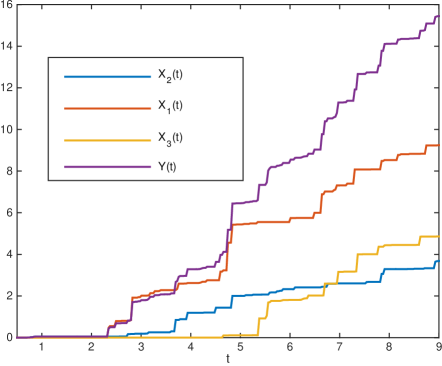
Figure 1: Degradation processes and a linear combination

3.2.1 First hitting time

To characterise the maintenance scheme of this system, the distribution of the hitting times of the process $\{Y(t),t\geq 0\}$ is obtained. Starting from $Y(0)=0$ and for a fixed degradation level $L$, the first hitting time $\sigma_{L}$ is defined as the amount of time required for the process $\{Y(t),t\geq 0\}$ to reach the degradation level $L$, that is,

$$\sigma_{L}=\textrm{inf}(t>0:Y(t)\geq L).$$

The distribution of $\sigma_{L}$ is obtained as

$$F_{\sigma_{L}}(t) =P(Y(t)\geq L)$$

$$=\int_{L}^{\infty}g_{Y(t)}(y)dy$$

$$=\int_{L}^{\infty}D(t)\sum_{k=0}^{\infty}\frac{\zeta_{k}(t)\beta_{0}^{-\rho(t)-k}}{\Gamma(\rho(t)+k)}y^{\rho(t)+k-1}e^{-y/\beta_{0}}dy$$

$$=D(t)\left(\sum_{k=0}^{\infty}\frac{\zeta_{k}(t)\beta_{0}^{-\rho(t)-k}}{\Gamma(\rho(t)+k)}\int_{L}^{\infty}y^{\rho(t)+k-1}e^{-y/\beta_{0}}dy\right)$$

$$=D(t)\sum_{k=0}^{\infty}\frac{\zeta_{k}(t)}{\Gamma(\rho(t)+k)}\Gamma_{\mathrm{ui}}(\rho(t)+k,L/\beta_{0}),$$ (9)

where $\Gamma_{\mathrm{ui}}(\rho(t)+k,L/\beta_{0})$ denotes the upper incomplete gamma function, which is given by

$$\Gamma_{\mathrm{ui}}(\rho(t)+k,L/\beta_{0})=\int_{L/\beta_{0}}^{\infty}z^{\rho(t)+k-1}e^{-z}dz.$$

We can link the probability distribution $F_{\sigma_{L}}(t)$ with the probability distribution of the hitting times for the processes $X_{k}(t)(k=1=2,...,n$ that compose $Y(t)$. That is, $F_{\sigma_{L}}(t)$ can be expressed by

$$F_{\sigma_{L}}(t)=D(t)\sum_{k=0}^{\infty}\zeta_{k}(t)F_{\sigma_{L,k}^{*}}(t),\quad t\geq 0,$$

where $F_{\sigma_{L,k}^{*}}(t)$ denotes the distribution of the first hitting time to exceed $L$ for a gamma process with parameters $\rho(t)+k$ and $\beta_{0}$, where $\rho(t)$ is given by (8) and $\beta_{0}=\min_{1\leq k\leq n}b_{k}\beta_{k}$.

3.3 The process of repair cost

Cost of repairing different effects, such as fatigue cracking and pavement deformation in a pavement network, may be different. Denote $c_{k,y}$ as the cost of repairing the $k$th defect with deterioration level $y$. We assume in this section that this cost is proportional to the deterioration level, that is, $c_{k,y}=yc_{k}$, where $c_{k}$ is the cost of repairing the $k$th defect per unit deterioration level. We define $U(t)=\sum_{k=1}^{n}c_{k}X_{k}(t)$ as the total repair cost at time $t$. Then $\{U(t),t\geq 0\}$ is the cost growth process and $c_{k}X_{k}(t)$ has pdf $f(x;\alpha_{k}(t),c_{k}\beta_{k})$. The expected value and the variance of $U(t)$ can be obtained by replacing $b_{k}$ with $c_{k}b_{k}$ in Eq. (4) and Eq. (5), respectively. The pdf of $U(t)=\sum_{k=1}^{n}c_{k}X_{k}(t)$ can be obtained via replacing $b_{k}$ with $c_{k}b_{k}$ in the pdf of $Y$ in Eq. (6).

The covariance between $Y(t)$ and $U(t)$ is given by

$$\textrm{Cov}(Y(t),U(t))=\sum_{k=1}^{n}\sum_{j=1}^{n}b_{k}c_{j}\textrm{cov}(X_{k}(t),X_{j}(t)).$$ (10)

Since $X_{k}(t)$ for $k=1,2,...$ are independent, $\textrm{cov}(X_{k}(t),X_{j}(t))=0$ for $k\neq j$, then

$$\textrm{Cov}(Y(t),U(t))=\sum_{k=1}^{n}b_{k}c_{k}\alpha_{k}(t)\beta_{k}^{2}(t).$$ (11)

In most existing research on maintenance cost of one degradation process $Y(t)$, once the magnitude of the degradation $Y(t)$ is given, the associated cost of repair may be $c_{r}Y(t)$, which is proportional to $Y(t)$ (where $c_{r}$ denotes the cost of repairing a unit of $Y(t)$). However, in our setting, $U(t)$ forms a stochastic process that is not proportional to $Y(t)$. This is because there are many different combinations of $Y_{k}(t)$ that can be summed up to obtain the same value of $Y(t)$. Correspondingly, the different $Y_{k}(t)$’s incur different repair cost $c_{k,y}$. As such, for a $Y(t)$ at a given time point $t$, its associated repair cost $U(t)$ is a random variable that does not have a linear correlationship with $Y(t)$.

The next result gives the distribution of the cost of repair, conditioning that the linear combination of the degradation processes exceeds the pre-specified value $L$.

Lemma 1

The conditional probability $f_{U(t)|Y(t)}(y,z)$ is given by

$$f_{U(t)|Y(t)}(y,u) =\frac{1}{4\pi^{2}g_{Y(t)}(y)}\int_{-\infty}^{\infty}\int_{-\infty}^{\infty}\left(\prod_{k=1}^{n}(1-i(b_{k}t_{1}+c_{k}t_{2})\beta_{k})^{-\alpha_{k}(t)}\right)e^{-it_{1}y-it_{2}u}\d{t}_{1}\d{t}_{2}.$$ (12)

Proof.  The characteristic function of the bivariate vector $(Y(t),U(t))$ is derived by

$$\phi_{Y(t),U(t)}(t_{1},t_{2}) =\mathbb{E}[\exp(it_{1}Y(t)+it_{2}U(t))]$$

$$=\mathbb{E}[\exp(it_{1}\sum_{k=1}^{n}b_{k}X_{k}(t)+it_{2}\sum_{k=1}^{n}c_{k}X_{k}(t))]$$

$$=\mathbb{E}[\exp(i\sum_{k=1}^{n}(b_{k}t_{1}+c_{k}t_{2})X_{k}(t)]$$

$$=\prod_{k=1}^{n}\mathbb{E}[\exp(i(b_{k}t_{1}+c_{k}t_{2})X_{k}(t)]$$

$$=\prod_{k=1}^{n}\phi_{X_{k}(t)}(b_{k}t_{1}+c_{k}t_{2}).$$ (13)

Since $\phi_{X_{k}(t)}(b_{k}t_{1}+c_{k}t_{2})=(1-i(b_{k}t_{1}+c_{k}t_{2})\beta_{k}^{-1})^{-\alpha_{k}(t)}$, we can obtain

$$f_{Y(t),U(t)}(y,u) =\frac{1}{4\pi^{2}}\int_{-\infty}^{\infty}\int_{-\infty}^{\infty}\phi_{Y(t),U(t)}(t_{1},t_{2})e^{-it_{1}y-it_{2}u}\d{t}_{1}\d{t}_{2}$$

$$=\frac{1}{4\pi^{2}}\int_{-\infty}^{\infty}\int_{-\infty}^{\infty}\left(\prod_{k=1}^{n}\phi_{X_{k}(t)}(b_{k}t_{1}+c_{k}t_{2})\right)e^{-it_{1}y-it_{2}u}\d{t}_{1}\d{t}_{2}$$

$$=\frac{1}{4\pi^{2}}\int_{-\infty}^{\infty}\int_{-\infty}^{\infty}\left(\prod_{k=1}^{n}(1-i(b_{k}t_{1}+c_{k}t_{2})\beta_{k}^{-1})^{-\alpha_{k}(t)}\right)e^{-it_{1}y-it_{2}u}\d{t}_{1}\d{t}_{2}.$$ (14)

Hence, the conditional probability $f_{U(t)|Y(t)}(y,u)$ is given by

$$f_{U(t)|Y(t)}(y,u) =\frac{f_{Y(t),U(t)}(y,u)}{g_{Y(t)}(y)}$$

$$=\frac{1}{4\pi^{2}g_{Y(t)}(y)}\int_{-\infty}^{\infty}\int_{-\infty}^{\infty}\left(\prod_{k=1}^{n}(1-i(b_{k}t_{1}+c_{k}t_{2})\beta_{k})^{-\alpha_{k}(t)}\right)e^{-it_{1}y-it_{2}u}\d{t}_{1}\d{t}_{2},$$ (15)

where $g_{Y(t)}(y)$ is given by (6). This establishes Lemma 1. $\blacksquare$

3.4 Incorporating random effect

It is known that random environment may affect the degradation processes of a system. For example, the deterioration processes of the defects on a pavement network may be affected by covariates such as the weather condition (the amount of rainfall) and traffic loading. If it is possible to collect weather condition data (eg., the amount of rainfall in a time period) and traffic loading data, one may incorporate co-variates in modelling. In addition, we may also consider random effects to account for possible model misspecification and individual unit variability.

[5] and [18] consider covariates in a gamma process. When incorporating covariates, represented by vector $z$, for example, [5] incorporate $\alpha_{k}(t)$ with $\alpha_{k}(te^{z^{\tau}\delta})$ (where $z^{\tau}$ is the transpose of $z$), [18] replace $\beta_{k}$ with $\beta_{k}(z)$, in which $z$ represents covariates and has the effect of rescaling X(t) without changing the shape parameter of its gamma distribution. $\beta_{k}(z)$ may have a regression function expression such as $\beta_{k}(z)=\exp(\boldsymbol{\beta^{\prime}z})$, where $\boldsymbol{\beta^{\prime}}$ and $\boldsymbol{z}$ are vectors of covariates and regression coefficients, respectively. In the following, we adopt the latter method and assume a degradation process $\{X^{\prime}_{k}(t),t\geq 0\}$, which takes both covariates and random effects into consideration. Then, $X^{\prime}_{k}(t)$ has density function $f_{\gamma}(x^{\prime};\alpha_{k}(t),w_{0}\beta_{z,k})$, where $w_{0}$ is a random effect and $\beta_{z,k}$ represents $\beta_{k}(z)$. One may assume that $w=w_{0}^{-1}$ has gamma distribution Gamma$(\gamma^{-1},\delta)$ and density function $g_{\gamma^{-1},\delta}(w)=\frac{\gamma^{\delta}}{\Gamma(\delta)}w^{\delta-1}e^{-\gamma w}$; $w$ has mean $\frac{\delta}{\gamma}$ and variance $\sigma^{2}_{z}=\frac{\delta}{\gamma^{2}}$. If $(X^{\prime}_{1},X^{\prime}_{2},\dots,X^{\prime}_{n},w_{0})$ has joint density $h(x_{1},x_{2},\dots,x_{n},w)$, then the conditional density of $X^{\prime}_{1},X^{\prime}_{2},\dots,X^{\prime}_{n}$ given $w_{0}=w$, is

$$h_{0}(x_{1},x_{2},\dots,x_{n}|w)=\frac{h(x_{1},x_{2},\dots,x_{n},w)}{g_{\gamma^{-1},\delta}(w)}.$$ (16)

For given weather conditions and traffic loading, one can regard $X_{1},X_{2},...,X_{n}$ as independent. That is, $X_{1}^{\prime},X_{2}^{\prime},...,X_{n}^{\prime}$ are conditionally independent given a third event. Then,

$$h(x_{1},x_{2},\dots,x_{n},w)= h_{0}(x_{1},x_{2},\dots,x_{n}|w)g_{\gamma^{-1},\delta}(w)$$

$$= g_{\gamma^{-1},\delta}(w)\prod_{k=1}^{n}h_{k}(x_{k}|w).$$ (17)

Since $h_{k}(x_{k}|w)=\frac{(\frac{\beta_{z,k}}{w})^{-\alpha_{k}(t)}}{\Gamma(\alpha_{k}(t))}x_{k}^{\alpha_{k}(t)-1}e^{-w\frac{x_{k}}{\beta_{z,k}}}$, if $(X^{\prime}_{1},X^{\prime}_{2},\dots,X^{\prime}_{n})$ has joint density function $f_{0}(x_{1},x_{2},\dots,x_{n})$, then

$$f_{0}(x_{1},x_{2},\dots,x_{n}) =\int_{0}^{+\infty}g_{\gamma^{-1},\delta}(w)\prod_{k=1}^{n}h_{k}(x_{k}|w)\d{w}$$

$$=\int_{0}^{+\infty}\left(\prod_{k=1}^{n}\frac{(\frac{\beta_{z,k}}{w})^{-\alpha_{k}(t)}}{\Gamma(\alpha_{k}(t))}x_{k}^{\alpha_{k}(t)-1}\right)e^{-w\sum_{k=1}^{n}\frac{x_{k}}{\beta_{z,k}}}g_{\gamma^{-1},\delta}(w)\d{w}$$

$$=\prod_{k=1}^{n}\frac{\beta_{z,k}^{-\alpha_{k}(t)}}{\Gamma(\alpha_{k}(t))}x_{k}^{\alpha_{k}(t)-1}\int_{0}^{\infty}\frac{\gamma^{\delta}}{\Gamma(\delta)}w^{\delta+\rho(t)-1}\exp\left\{-w\left(\gamma+\sum_{k=1}^{n}\frac{x_{k}}{\beta_{z,k}}\right)\right\}\d{w}$$ (18)

$$=\int_{0}^{\infty}\frac{\gamma^{\delta}}{\Gamma(\delta)}w^{\delta+\rho(t)-1}exp\left\{-w\left(\gamma+\sum_{k=1}^{n}\frac{x_{k}}{\beta_{z,k}}\right)\right\}\d{w}\left(\prod_{k=1}^{n}\frac{\beta_{z,k}^{-\alpha_{k}(t)}}{\Gamma(\alpha_{k}(t))}x_{k}^{\alpha_{k}(t)-1}\right)$$ (19)

$$=\frac{\gamma^{\delta}}{\Gamma(\delta)}\left(\gamma+\sum_{k=1}^{n}\frac{x_{k}}{\beta_{z,k}}\right)^{\delta+\rho(t)}\Gamma(\delta+\rho(t))\left(\prod_{k=1}^{n}\frac{\beta_{z,k}^{-\alpha_{k}(t)}}{\Gamma(\alpha_{k}(t))}x_{k}^{\alpha_{k}(t)-1}\right).$$ (20)

where $\rho(t)=\sum_{k=1}^{n}\alpha_{k}(t)$.

3.4.1 First hitting time

Next, we compute the first hitting time of the process $\left\{Y(t),t\geq 0\right\}$ to exceed a degradation level $L$. Let

$$\sigma_{L}=\textrm{inf}(t>0:Y(t)\geq L).$$

Then the probability distribution of $F_{\sigma_{L}}$ is given by

$$F_{\sigma_{L}}(t)= \sum_{k=1}^{n}b_{k}X_{k}(t)\geq L\int_{0}^{+\infty}g_{\gamma^{-1},\delta}(w)\prod_{k=1}^{n}h_{k}(x_{k}|w)dwdx_{1}...dx_{n}$$

$$= \sum_{k=1}^{n}b_{k}X_{k}(t)\geq L\int_{0}^{+\infty}\left(\prod_{k=1}^{n}\frac{(\frac{\beta_{z,k}}{w})^{-\alpha_{k}(t)}}{\Gamma(\alpha_{k}(t))}x_{k}^{\alpha_{k}(t)-1}\right)e^{-w\sum_{k=1}^{n}\frac{x_{k}}{\beta_{z,k}}}g_{\gamma^{-1},\delta}(w)dwdx_{1}...dx_{n}$$

$$= \int_{0}^{+\infty}\left(\sum_{k=1}^{n}b_{k}X_{k}(t)\geq L\left(\prod_{k=1}^{n}\frac{(\frac{\beta_{z,k}}{w})^{-\alpha_{k}(t)}}{\Gamma(\alpha_{k}(t))}x_{k}^{\alpha_{k}(t)-1}\right)e^{-w\sum_{k=1}^{n}\frac{x_{k}}{\beta_{z,k}}}dx_{1}...dx_{n}\right)g_{\gamma^{-1},\delta}(w)dw.$$ (21)

According to [20], we have

$$\sum_{k=1}^{n}b_{k}X_{k}(t)<L\left(\prod_{k=1}^{n}\frac{(\frac{\beta_{z,k}}{w})^{-\alpha_{k}(t)}}{\Gamma(\alpha_{k}(t))}x_{k}^{\alpha_{k}(t)-1}\right)e^{-w\sum_{k=1}^{n}\frac{x_{k}}{\beta_{z,k}}}g_{\gamma^{-1},\delta}(w)dwdx_{1}...dx_{n}=\int_{L}^{\infty}g_{Y(t)}^{\prime}(x)\d{x},$$

where $g_{Y(t)}^{\prime}(x)$ is obtained following the same reasoning as in (6), that is,

$$g_{Y(t)}^{\prime}(x)=D_{z}(t)\sum_{k=0}^{\infty}\frac{\zeta_{z,k}(t)(\beta_{z,0}/w)^{-\rho_{z}(t)-k}}{\Gamma(\rho_{z}(t)+k)}x^{\rho_{z}(t)+k-1}e^{-wx/\beta_{z,0}},$$

and $D_{z}(t)$, $\zeta_{z,k}(t)$, $\rho_{z}(t)$ and $\beta_{z,0}$ are obtained by replacing $\beta_{k}$ with $\beta_{z,k}$ in the definitions of $D(t)$, $\zeta_{k}(t)$, $\rho(t)$ and $\beta_{0}$, respectively.

Finally, we obtain

$$P(Y(t)\geq L)= \int_{0}^{\infty}\int_{L}^{\infty}g_{Y(t)}^{\prime}(y)g_{\gamma^{-1},\delta}(w)\d{y}\d{w}$$

$$= D_{z}(t)\gamma^{\delta}\sum_{k=0}^{\infty}\frac{\zeta_{z,k}(t)\beta_{z,0}^{-\rho_{z}(t)-k}}{B(\rho_{z}(t)+k,\delta)}\int_{L}^{\infty}x^{\rho_{z}(t)+k-1}\left(\gamma+\frac{x}{\beta_{z,0}}\right)^{\rho_{z}(t)+k+\delta}\d{x}$$

$$= D_{z}(t)(\beta_{z,0}\gamma)^{\delta}\sum_{k=0}^{\infty}\frac{\zeta_{z,k}(t)}{B(\rho_{z}(t)+k,\delta)}\int_{L}^{\infty}x^{\rho_{z}(t)+k-1}\left(\beta_{z,0}\gamma+x\right)^{\rho_{z}(t)+k+\delta}\d{x},$$ (22)

where $B(x,y)$ denotes the function beta given by

$$B(x,y)=\frac{\Gamma(x)\Gamma(y)}{\Gamma(x+y)}.$$

4 Maintenance Policies

In the reliability literature, there are many models describing the effectiveness of a maintenance activity. Such models include modification of intensity models [12], [29], reduction of age models [16],[12],[29], geometric processes [17],[30],[28], etc. For a system like a section of pavement, maintenance may remove all of the defects, the degradation processes of the defects may therefore stop. After maintenance, new defects may develop in a faster manner than before. The effectiveness of such maintenance may be modelled by the geometric process.

The geometric process describes a process in which the lifetime of a system becomes shorter after each maintenance. Its definition is given by [17], and it is shown below.

Definition 1

[17] Given a sequence of non-negative random variables $\{X_{j},j=1,2,\dots\}$, if they are independent and the cdf of $X_{j}$ is given by $F(a^{j-1}x)$ for $j=1,2,\dots$, where $a$ is a positive constant, then $\{X_{j},j=1,2,\cdots\}$ is called a geometric process (GP).

The parameter $a$ in the GP plays an important role. The lifetime described by $F(a^{j-1}x)$ with a larger $a$ is shorter than that described by $F(a^{j-1}x)$ with a smaller $a$ with $j=1,2,\ldots$.

• If $a>1$, then $\{X_{j},j=1,2,\cdots\}$ is stochastically decreasing.

• If $a<1$, then $\{X_{j},j=1,2,\cdots\}$ is stochastically increasing.

• If $a=1$, then $\{X_{j},j=1,2,\cdots\}$ is a renewal process.

• If $\{X_{j},j=1,2,\dots\}$ is a GP and $X_{1}$ follows the gamma distribution, then the shape parameter of $X_{j}$ for $j=2,3,\dots$ remains the same as that of $X_{1}$ but its scale parameter changes.

GP has been used extensively in the reliability literature to implement the effect of imperfect repairs on a repairable system (see [9], [27], [30], [28], among others).

In addition to the assumptions listed in Section 2, we make the following assumptions.

1. Immediately after a repair, the system resets its age to 0, at which there are no defects in the system.

2. The initiation of the defects after the $j$-th imperfect repair follows a homogeneous Poisson process with parameters $\lambda/a_{1}(T)^{j-1}$ with $a_{1}(T)>0$ and $a_{1}(T)$ being a non-decreasing function in $T$ for $j=1,2,\ldots$.

3. After the $j$-th repair and after the arrival of the $k$-th defect, the $k$-th defect grows according to a gamma process with shape parameter $\alpha_{k}(t)$ and scale parameter $a_{2}(T)^{j-1}\beta_{k}$ with $a_{2}(T)(>0)$ being $a_{2}(T)$ an increasing function in $T$ for $j=1,2,\ldots$.

4. Each inspection implies a cost of $c_{I}$ monetary units, $c_{k,y}$ corresponds to the variable cost of repairing the $k$-th defect with degradation level equals to $y$ and $c_{f,k}$ corresponds to the fixed cost of repairing the $k$-th defect. Furthermore, if in an inspection time the “overall degradation” of the system given by (23) exceeds the threshold $L$, an additional cost of $c_{F}$ monetary units is incurred. The cost of the replacement at time $NT$ is equal to $c_{R}$.

We explain assumptions A9) and A10), respectively, in the following.

• Assumption A9) implies that the defect arrival rate relates to the inspection interval $T$, which reflects the case that $a_{1}(T)$ becomes bigger and the system tends to deteriorate faster for large $T$ than for small $T$.

• Assumption A10) implies that the degradation rate increases with the number of imperfect repairs performed on the system. We denote by $\left\{Y^{*}_{j}(t),t\geq 0\right\}$ the “overall” degradation of the maintained system after the $j$-th repair, and denote

  $$Y^{*}_{j}(t)=\sum_{k=1}^{n}b_{k}X_{k,j}(t),\quad 0\leq t\leq T,$$ (23)

  where $\left\{X_{k,j}(t),t\geq 0\right\}$ stands for a gamma process with parameters $\alpha_{k}$ and $\beta_{k}a_{2}(T)^{j-1}$. Similar to the derivation process shown in previous section, we can compute the first hitting time to exceed the threshold $L$ for the process (23) following the same reasoning as in (6) replacing $\beta_{k}$ by $\beta_{k}a_{2}(T)^{j-1}$. That is,

  $$\sigma_{L}^{(j)}=\inf\left\{t\geq 0:Y^{*}_{j}(t)\geq L\right\},$$

  and we denote by $F_{\sigma_{L}}^{j}$ the distribution of $\sigma_{L}^{(j)}$.

The problem is to determine the time between inspections and the number of inspections that minimise an objective cost function. The optimisation problem is formulated in terms of the expected cost rate per unit time.

By a replacement cycle, we mean the time between two successive replacements of the system. In this paper, the total replacement cycle is equal to $NT$. Let $\mathrm{Q}_{0}(N,T)$ be the expected rate of the total cost in a replacement cycle. Then we obtain

$$\mathrm{Q}_{0}(N,T)= \frac{1}{NT}\sum_{j=1}^{N}\left[c_{I}+\sum_{k=1}^{n}\frac{(a_{1}(T))^{j-1}}{\lambda}\left(c_{f,k}+\int_{0}^{\infty}c_{k,y}f(y;\alpha_{k}(T),\beta_{k}a_{2}(T)^{j-1})\d{y}\right)\right.$$

$$\left.+c_{F}\frac{(a_{1}(T))^{j-1}}{\lambda}F_{\sigma_{L}}^{j}(T)\right]+\frac{c_{R}}{NT},$$ (24)

where $f(y;\alpha_{k}(T),\beta_{k}a_{2}(T)^{j-1})$ is given by (2) and $F_{\sigma_{L}}^{j}(T)$ is given by (9) replacing $\beta_{k}$ by $\beta_{k}a_{2}(T)^{j-1}$. The expected variable cost per unit time in a replacement cycle is given by

$$\mathrm{CV}(N,T)=\frac{1}{NT}\sum_{j=1}^{N}\sum_{k=1}^{n}\frac{a_{1}(T)^{j-1}}{\lambda}\int_{0}^{\infty}c_{k,y}f(y;\alpha_{k}(T),\beta_{k}a_{2}(T)^{j-1})\d{y}.$$ (25)

The optimization problem is formulated as

$$\mathrm{Q}_{0}(N_{opt},T_{opt})=\min_{\begin{subarray}{c}N=1,2,...\\ T>0\end{subarray}}\mathrm{Q}_{0}(N,T).$$ (26)

4.1 Special cases

In this section, we discuss $\mathrm{Q}_{0}(N,T)$ and $\mathrm{CV}(N,T)$ under special cases of $c_{k,y}$, $a_{1}(T)$, $a_{2}(T)$, and $\alpha_{k}(T)$, respectively.

4.1.1 Special cases of $c_{k,y}$

Different scenarios can be envisaged depending on the variable cost function $c_{k,y}$.

• If $c_{k,y}=c_{k}$, then the expected variable cost rate (25) in a renewal cycle is given by

  $$\mathrm{CV}(N,T) =\frac{1}{NT}\sum_{j=1}^{N}\sum_{k=1}^{n}\frac{a_{1}(T)^{j-1}}{\lambda}\int_{0}^{\infty}c_{k}f(y;\alpha_{k}(T),\beta_{k}a_{2}(T)^{j-1})\d{y}$$

  $$=\frac{1}{NT}\sum_{j=1}^{N}\sum_{k=1}^{n}\frac{a_{1}(T)^{j-1}c_{k}}{\lambda}.$$

• If $c_{k,y}$ is directly proportional to the degradation level of the $k$-th defect in the inspection time, that is, $c_{k,y}=yc_{k}$, then the expected variable cost (25) is equal to

  $$\mathrm{CV}(N,T) =\frac{1}{NT}\sum_{j=1}^{N}\sum_{k=1}^{n}\frac{a_{1}(T)^{j-1}}{\lambda}\int_{0}^{\infty}c_{k}yf(y;\alpha_{k}(T),\beta_{k}a_{2}(T)^{j-1})\d{y}$$

  $$=\frac{1}{NT}\sum_{j=1}^{N}\sum_{k=1}^{n}\frac{a_{1}(T)^{j-1}}{\lambda}c_{k}\alpha_{k}(T)a_{2}(T)^{j-1}\beta_{k}$$

  $$=\frac{1}{NT}\left(\frac{(a_{1}(T)a_{2}(T))^{N}-1}{a_{1}(T)a_{2}(T)-1}\right)\sum_{k=1}^{n}\frac{c_{k}\alpha_{k}(T)\beta_{k}}{\lambda}.$$

• If $c_{k,y}$ is directly proportional to the square of the degradation level of the $k$-th defect in the inspection time, that is, $c_{k,y}=y^{2}c_{k}$. In this case, the repair cost may relate to the area of a defect, see [26], for example. (25) is given by

  $$\mathrm{CV}(N,T) =\frac{1}{NT}\sum_{j=1}^{N}\sum_{k=1}^{n}\frac{a_{1}(T)^{j-1}}{\lambda}\int_{0}^{\infty}c_{k}y^{2}f(y;\alpha_{k}(T),\beta_{k}a_{2}(T)^{j-1})\d{y}$$

  $$=\frac{1}{NT}\sum_{j=1}^{N}\sum_{k=1}^{n}\frac{a_{1}(T)^{j-1}}{\lambda}c_{k}\left(\mathrm{Var}(X_{k,j}(T))+(\mathbb{E}(X_{k,j}(T)))^{2}\right)$$

  $$=\frac{1}{NT}\sum_{j=1}^{N}\sum_{k=1}^{n}\frac{a_{1}(T)^{j-1}}{\lambda}c_{k}\left(\beta_{k}^{2}\alpha_{k}(T)a_{2}(T)^{2j-2}+\beta_{k}^{2}\alpha_{k}(T)^{2}a_{2}(T)^{2j-2}\right)$$

  $$=\frac{1}{NT}\left(\frac{(a_{1}(T)a_{2}(T)^{2})^{N}-1}{a_{1}(T)a_{2}(T)^{2}-1}\right)\sum_{k=1}^{n}\frac{c_{k}\beta_{k}^{2}(\alpha_{k}(T)+\alpha_{k}(T)^{2})}{\lambda}.$$

4.1.2 Special cases of $a_{1}(T)$, $a_{2}(T)$, and $\alpha_{k}(T)$

The analysis of the monotonicity of $\mathrm{Q}_{0}(N,T)$ is quite tricky. To analyse it, some particular conditions are imposed. We assume that $a_{1}(T)=a_{1}$, $a_{2}(T)=a_{2}$, $\alpha_{k}(T)=\alpha_{k}T$, and $c_{k,y}=yc_{k}$, $\mathrm{Q}_{0}(N,T)$ given by (24) is then reduced to

$$\mathrm{Q}_{0}(N,T) =\frac{c_{I}}{T}+\frac{c_{R}}{NT}+\frac{(a_{1}^{N}-1)}{(a_{1}-1)\lambda NT}\sum_{k=1}^{n}c_{f,k}$$ (27)

$$+\frac{(a_{1}^{N}a_{2}^{N}-1)}{\lambda N(a_{1}a_{2}-1)}\sum_{k=1}^{n}c_{k}\alpha_{k}\beta_{k}+\frac{c_{F}}{\lambda NT}\sum_{j=1}^{N}a_{1}^{j-1}F_{\sigma_{L}}^{(j)}(T).$$

We suppose that $N$ is constant and $T$ is variable on $(0,\infty)$. A necessary condition that a finite $T^{*}$ minimises $\mathrm{Q}_{0}(N,T)$ given by (27) is that it satisfies

$$\sum_{j=1}^{N}a_{1}^{j-1}\left(f_{\sigma_{L}}^{(j)}(T)T-F_{\sigma_{L}}^{(j)}(T)\right)=\frac{\lambda}{c_{F}}\left(Nc_{I}+\frac{a_{1}^{N}-1}{\lambda(a_{1}-1)}\sum_{k=1}^{n}c_{f,k}+c_{R}\right).$$

Next, we suppose that $T$ is constant. Then a necessary condition that there exists a finite a unique $N^{*}$ minimizing $\mathrm{Q}_{0}(N,T)$ is that $N^{*}$ satisfies

$$\mathrm{Q}_{0}(N+1,T)\geq\mathrm{Q}_{0}(N,T),$$

and

$$\mathrm{Q}_{0}(N,T)\geq\mathrm{Q}_{0}(N-1,T).$$

We get that

$$\mathrm{Q}_{0}(N+1,T)-\mathrm{Q}_{0}(N,T)= \frac{1}{\lambda T(a_{1}-1)}\sum_{k=1}^{n}c_{f,k}\frac{N(a_{1}^{N+1}-a_{1}^{N})-a_{1}^{N}+1}{N(N+1)}$$

$$+\frac{\sum_{k=1}^{n}c_{k}\alpha_{k}\beta_{k}}{\lambda(a_{1}a_{2}-1)}\frac{N(a_{1}^{N+1}a_{2}^{N+1}-a_{1}^{N}a_{2}^{N})-a_{1}^{N}a_{2}^{N}+1}{N(N+1)}$$

$$-\frac{c_{R}}{N(N+1)T}+c_{F}\frac{\sum_{j=1}^{N}a_{1}^{N}F_{\sigma_{L}}^{(N+1)}(T)-a_{1}^{j-1}F_{\sigma_{L}}^{(}j)(T)}{\lambda N(N+1)T}.$$

Hence, for fixed $T$, $\mathrm{Q}_{0}((N+1),T)-\mathrm{Q}_{0}(N,T)\geq 0$ if and only if

$$c_{R}<D(N,T),$$

where

$$D(N,T) =\frac{1}{\lambda}\sum_{k=1}^{n}c_{f,k}\frac{N(a_{1}^{N+1}-a_{1}^{N})-a_{1}^{N}+1}{(a_{1}-1)}$$

$$+T\sum_{k=1}^{n}c_{k}\alpha_{k}\beta_{k}\frac{N(a_{1}^{N+1}a_{2}^{N+1}-a_{1}^{N}a_{2}^{N})-a_{1}^{N}a_{2}^{N}+1}{\lambda(a_{1}a_{2}-1)}$$

$$+\frac{c_{F}}{\lambda}\left(\sum_{j=1}^{N}a_{1}^{N}F_{\sigma_{L}}^{(N+1)}(T)-a_{1}^{j-1}F_{\sigma_{L}}^{(j)}(T)\right).$$

We get that, if $a_{1}>2$, then $D(N,T)$ is non decreasing in $N$. Therefore, if

$$c_{R}<D(1,T),$$

then $c_{R}<D(N,T)$ for all $N$. We get that

$$D(1,T) =\frac{(a_{1}-1)}{\lambda}\sum_{k=1}^{n}c_{f,k}+\frac{T(a_{1}a_{2}-1)}{\lambda}\sum_{k=1}^{n}c_{k}\alpha_{k}\beta_{k}+\frac{c_{F}}{\lambda}\left(a_{1}F_{\sigma_{L}}^{(2)}(T)-F_{\sigma_{L}}^{(1)}(T)\right).$$

Hence, if $a_{1}>2$ and

$$c_{R}<\frac{(a_{1}-1)}{\lambda}\sum_{k=1}^{n}c_{f,k},$$

then $\mathrm{Q}_{0}(N,T)$ is increasing in $N$.

An economic constraint is introduced in the optimisation problem formulated in (26) to limit the variable cost in a replacement cycle. The introduction of constraints in the search of the optimal maintenance strategy is not new in the literature. For example, [3] and [4] introduced constraints related to the system safety in an optimisation problem. In this paper, the constraint imposed in the optimisation is economic and it is related to the expected variable cost imposing that this expected variables cost cannot exceed a threshold K.

Let $\Omega$ be the set of pairs $(N,T)$ such that $\mathrm{CV}(N,T)\leq K$, that is,

$$\Omega=\left\{(N,T):N=1,2,\ldots,T>0\,\,\mbox{subject to}\,\,\mathrm{CV}(N,T)\leq K\right\},$$ (28)

and the optimisation problem is formulated in terms of the economic constraint as

$$\mathrm{Q}_{0}^{*}(T_{opt},N_{opt})=\inf\left\{\mathrm{Q}_{0}(N,T):(N,T)\in\Omega\right\}.$$ (29)

To analyse the optimisation problem given by (29), the monotonicity of the function $\mathrm{CV}(N,T)$ is studied.

4.2 Economic constraint analysis

We analyse the monotonicity of $\mathrm{CV}(N,T)$ in the two variables $N$ and $T$ and assume that $c_{k,y}=yf(y;\alpha_{k}(T),\beta)$ (i.e., variable cost proportional to the degradation level) and $a_{2}(T)>1$ and $a_{1}(T)>1$ for all $T$.

Lemma 2

If $\alpha_{k}(T)$ is convex in $T$ for all $k$ with $\alpha_{k}(0)=0$ and $\alpha_{k}^{\prime}(0)<\infty$, then

• $\mathrm{CV}(N,T)$ is increasing in $T$ for fixed $N$, and

• $\mathrm{CV}(N,T)$ is increasing in $N$ for fixed $T$.

Proof.  The expected variable cost rate is given by

$$\mathrm{CV}(N,T) =\frac{1}{N}\left(\sum_{k=1}^{n}\frac{c_{k}\beta_{k}\alpha_{k}(T)/T}{\lambda}\right)\left(\sum_{j=0}^{N-1}(a_{1}(T)a_{2}(T))^{j}\right)$$

$$=\frac{1}{N}\frac{(a_{1}(T)a_{2}(T))^{N}-1}{a_{1}(T)a_{2}(T)-1}\left(\sum_{k=1}^{n}\frac{c_{k}\beta_{k}\alpha_{k}(T)/T}{\lambda}\right).$$ (30)

The function $\alpha_{k}(T)/T$ is increasing in $T$ as consequence of the convexity of $\alpha_{k}(T)$ along with $\alpha_{k}(0)=0$ and $\alpha_{k}^{\prime}(0)<\infty$. On the one hand, since $a_{1}(T)$ and $a_{2}(T)$ are increasing in $T$, $\mathrm{CV}(N,T)$ is increasing in $T$. On the other hand, the function

$$g(N)=\frac{1}{N}\sum_{j=1}^{N-1}(a_{1}(T)a_{2}(T))^{j},$$

is increasing in $N$ since

$$g(N+1)-g(N)=\frac{\sum_{j=0}^{N-1}((a_{1}(T)a_{2}(T))^{N}-(a_{1}(T)a_{2}(T))^{j})}{N(N+1)},$$

and $a_{1}(T)a_{2}(T)>1$, hence $\mathrm{CV}(N,T)$ is increasing in $N$. This establishes Lemma 2. $\blacksquare$

The first consequence of Lemma 2 is that the condition

$$\frac{1}{\lambda}\sum_{k=1}^{n}c_{k}\beta_{k}\lim_{T\rightarrow 0}\frac{\alpha_{k}(T)}{T}\leq K,$$ (31)

has to be imposed. If inequality (31) is not fulfilled, then $\Omega=\emptyset$. On the other hand, if

$$\lim_{T\rightarrow\infty}\lim_{N\rightarrow\infty}\mathrm{CV}(N,T)\leq K,$$ (32)

then $\Omega=\left\{{\color[rgb]{0,0,0}(N,T):}T>0,\,N=1,2,\ldots\right\},$ and the optimisation problem in (29) is reduced to the optimisation problem in (26). Hence, to deal with the optimisation problem with constraints, we assume that the following inequality

$$\frac{1}{\lambda}\sum_{k=1}^{n}c_{k}\beta_{k}\lim_{T\rightarrow 0}\frac{\alpha_{k}(T)}{T}\leq K<\lim_{T\rightarrow\infty}\lim_{N\rightarrow\infty}\mathrm{CV}(N,T),$$ (33)

is fulfilled. If (33) is fulfilled, we denote

$$N_{1}=\inf\left\{N:\lim_{T\rightarrow\infty}\mathrm{CV}(N,T)>K\right\},$$

and

$$N_{2}=\inf\left\{N:\lim_{T\rightarrow 0}\mathrm{CV}(N,T)>K\right\}.$$

We obtain that $N_{1}\leq N_{2}$.

If $N^{*}$ is fixed such that $N_{1}\leq N^{*}\leq N_{2}$, we denote $T_{N}^{*}$ as the root of the equation

$$\mathrm{CV}(N^{*},T_{N}^{*})=K,$$

and the set $\Omega$ given in (28) is therefore equal to

$$\Omega=\left\{(N,T):N=1,2,\ldots,N_{1}-1\right\}\cup\left\{(N,T):N=N_{1},N_{1}+1,\ldots,N_{2}-1,\,T\leq T_{N}^{*}\right\}.$$ (34)

5 Numerical examples

We consider a system subject to three different defects, all of which start at random times, following a homogeneous Poisson process with rate $\lambda=1$ defects per unit time. The degradation process of the three defects is modelled using a nonhomogeneous gamma processes with shape parameters $\alpha_{k}(t)=\alpha_{k}t^{\xi_{k}}$ with $\xi_{k}=2$, $\alpha_{1}=1$, $\alpha_{2}=1$, $\alpha_{3}=1$ and scale parameters $\beta_{1}=1$, $\beta_{2}=2$ and $\beta_{3}=3$, respectively. The random effect $w_{0}$ is modelled with $w=w_{0}^{-1}$, where $w$ follows a gamma distribution $Gamma(1,2)$.

The overall degradation process of the system $Y$ is a combination linear of the three processes

$$Y=0.2X_{1}+0.7X_{2}+0.4X_{3},$$

and we assume that the system fails when the degradation level of $Y$ exceeds the failure threshold $L=20$. Imperfect repairs are performed on the system every $T$ time units and the effect of these imperfect repairs is modelled by a geometric process with parameters $a_{1}(T)=1.1(1.2-0.2\exp(-T))$ for the time between arrivals and $a_{2}(T)=1.15(1.2-0.2\exp(-T))$ for the effect of the imperfect repairs on the degradation rate of the defects. Each inspection involves a cost of $c_{I}=0.05$ monetary units. Each repair involves a fixed cost of $c_{f,1}=2$ monetary units for the first defect, $c_{f,2}=2$ monetary units for the second defect and $c_{f,3}=2$ monetary units for the third defect. Each repair involves also a variable cost depending on the degradation of the defect. The variable cost is given by $c_{1,y}=7y$, $c_{2,y}=7y$ and $c_{3,y}=7y$ on the three defects, respectively, where $y$ denotes the degradation of the defect in the time of the repair. If the overall degradation of the system exceeds $L=20$ in the repair time, an additional cost of $c_{F}=100$ monetary units is incurred. A complete replacement of the system by a new one is performed at the time of the $N$-th imperfect repair with a cost of $c_{R}=1000$ monetary units.

Figure 2 shows the expected cost per unit time $\mathrm{Q}_{0}(N,T)$ versus $N$ and $T$. This graphic is obtained by simulation with 10 values for $T$ from 1 to 7, $N$ from 1 to 2 and 3000 simulations in each point.

By inspection, the minimal value of $\mathrm{Q}_{0}(N,T)$ are obtained for $T_{opt}=1.9474$ and $N_{opt}=3$ with and optimal expected cost rate of $\mathrm{Q}_{0}(N_{opt},T_{opt})=332.6066$ monetary units per unit time.

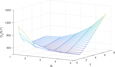
Figure 2: Expected cost $\mathrm{Q}_{0}(N,T)$ versus $N$ and $T$.

The economic safety constraint is introduced in this problem and it is dependent on the variable cost given by

$$\mathrm{CV}(N,T)=\frac{1}{\lambda N}\sum_{k=1}^{n}c_{k}\alpha_{k}\beta_{k}T\sum_{j=0}^{N-1}(a_{1}(T)a_{2}(T))^{j}.$$ (35)

For fixed $N$, the function given by (35) is non-decreasing in $T$. For fixed $T$, we get that

$$\mathrm{CV}(N+1,T)-\mathrm{CV}(N,T)=\sum_{k=1}^{n}\frac{c_{k}\alpha_{k}\beta_{k}T}{\lambda}\sum_{j=0}^{N-1}\frac{\left((a_{1}(T)a_{2}(T))^{N}-a_{1}(T)a_{2}(T)^{j}\right)}{N(N+1)},$$

is positive. Figure 3 shows the economic safety constraint versus $T$ and $N$.

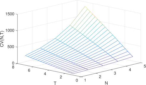
Figure 3: Variable cost $\mathrm{CV}(N,T)$ versus $N$ and $T$.

As we visually can check, the variable cost is non-decreasing in $N$ for fixed $T$ and non-decreasing in $T$ for fixed $N$.

We assume that the variable cost cannot exceed the threshold $K=130$ monetary units, that is, the optimization of $\mathrm{Q}_{0}(N,T)$ given by (24) is performed on the set $\Omega_{1}$, where

$$\Omega_{1}=\left\{(N,T)\;\;\mbox{such that}\;\;\,\mathrm{CV}(N,T)\leq 130\right\}.$$

Inequality (33) is fulfilled since

$$\lim_{T\rightarrow 0}\mathrm{CV}(1,T)=\lim_{T\rightarrow 0}\frac{1}{\lambda}\sum_{k=1}^{n}c_{k}\beta_{k}\alpha_{k}T^{\xi_{k}-1}=0,$$

and, therefore, $\lim_{T\rightarrow 0}\mathrm{CV}(1,T)\leq K$, and

$$\lim_{N\rightarrow\infty}\lim_{T\rightarrow\infty}\mathrm{CV}(N,T)=\infty,$$

hence inequality (33) is fulfilled.

Figure 4 shows the value of $\mathrm{CV}(N,T)$ for $N\leq 10$.

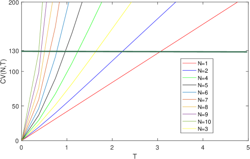
Figure 4: Variable cost $\mathrm{CV}(N,T)$ versus $T$.

The set of the points $\Omega$ that fulfils the economic constraint is given by

$$\Omega_{1}=\left\{(N,T),\,N\geq 1;\quad T\leq T_{N}^{*}\right\},$$

where $T_{N}^{*}$ is the root of $\mathrm{CV}(N,T)=K$.

The point in which the global minimum is obtained in the unconstrained problem (that is, $T_{opt}=1.9474$ and $N_{opt}=3$) presents a variable cost equals to $\mathrm{CV}(N_{opt},T_{opt})=147.8725$ monetary units per unit time what it implies that it is not an optimal solution for the constrained problem.

Figure 5 shows the values for the expected cost rate $\mathrm{Q}_{0}(N,T)$ for $T\leq T_{N}^{*}$, that is, the expected cost rate $\mathrm{Q}_{0}(N,T)$ in the subset $\Omega$. The minimum of these function is reached at point $N_{opt}=4$ and $T_{opt}=1.1137$ with an expected cost rate equals to $\mathrm{Q}_{0}(T_{opt},N_{opt})=344.4153$ monetary units per unit time.

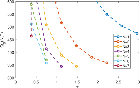
Figure 5: Expected cost rate $\mathrm{Q}_{0}(N,T)$ versus $T$ in $\Omega$.

6 Discussion

This paper discussed the scenario where a linear combination of degradation processes was studied. Below we discuss the assumption of the degradation processes, the random environment, and the effectiveness of repair.

6.1 Degradation process.

The preceding sections assume that $X_{k}(t)$ follows the gamma process. Certainly, one may choose the degradation process of $X_{k}(t)$ based on the real applications: for example, in the case of the example investigated in this paper, the propagation process of a fatigue crack evolves monotonically only in one direction, the gamma process is a good choice. Methodologically, however, $X_{k}(t)$ may be assumed to follow any other process, such as the Wiener process [25], the inverse Gaussian process [10] and the Ornstein-Uhlenbeck process [11]. The probability distribution of $\sum_{k=1}^{n}X_{k}(t)$ can be easily derived if $X_{k}(t)(k=1,2,...,n)$ follow Wiener processes. In some case, a closed form of the distribution of $\sum_{k=1}^{n}X_{k}(t)$ may not be easily found and therefore numerical methods may be pursued.

One may also assume that $X_{k}(t)$ may follow different degradation processes, for example, on different $k$’s, some $X_{k}(t)$’s follow gamma processes and others follow Wiener processes.

6.2 Incorporation of dynamic environments.

The system considered in this paper is operated under a random environment. In addition to the method that incorporate the random environment with the random effect method, one may also use other methods, for example, one may consider the effect of the dynamic environment on the system as external shocks using Poisson processes [31], or as other stochastic processes, including continuous-time Markov chain process [6], and Semi-Markov process [15]. The reader is referred to [21] for a discussion in detail.

6.3 Imperfect repair.

In this paper, we consider the effectiveness of repair as imperfect. The justification is as follows. If we consider a pavement network, all defects, such as fatigue cracking and pavement deformation, disappear after repair. This does not suggest the pavement network is repaired as good as new (i.e., perfect repair) or as bad as old (i.e., minimal repair). Instead, it is more reasonable to assume that the repair is imperfect. In the literature, many methods that model the effectiveness of imperfect maintenance have been developed (see the Introduction section in [29], for example). For simplicity, this paper uses the geometric process introduced in [17]. Of course, one may other models such as the age-modification models [16],[12], under which the optimisation process becomes much more complicated.

6.4 Maintenance policy based on the cost process.

Since $U(t)$ forms a stochastic process, one may develop a maintenance policy based on the cost process. That is, once the cost process reaches a threshold, maintenance on the combined degradation process $Y(t)$ is carried out. Hence, intriguing questions may include optimisation of maintenance intervals, for example.

6.5 Rethinking of the assumptions

The above sections assumes the defect inter-occurrence times to be exchangeable and to exhibit the lack of memory property. Nevertheless, both properties may be violated in the real world. If so, one may assume that the defect inter-occurrence times follow a non-homogeneous Poisson process, for example.

6.6 A $r$-out-of-$n$ case

In Section 3.2, we discussed the case when the sum of the deterioration levels is monitored. In practice, another scenario may be to monitor $r$-out-of-$n$ deterioration processes. That is, if $k$-out-of-$n$ deterioration levels are greater than their pre-specified thresholds, respectively, maintenance needs performing. Denote $Y_{(1)}(t),Y_{(3)}(t),...,Y_{(n)}(t)$ as by sorting the values (realisations) of $Y_{1}(t),Y_{2}(t),...,Y_{n}(t)$ in increasing order. For simplicity, we assume that $Y_{k}(t)$ are i.i.d for $k=1,2,...,n$ with cdf $F(x,\alpha(t),b^{-1}\beta)$. The cumulative distribution function of $Y_{(r)}(t)$ is given by

$$G_{Y_{(r)}(t)}(y)=1-\sum_{k=r}^{n}\frac{n!}{(n-r)!r!}(1-F(y,\alpha(t),b^{-1}\beta))^{k}(F(y,\alpha(t),b^{-1}\beta))^{n-k}.$$ (36)

First hitting time $T_{L_{2}}$. Let $T_{L_{2}}=\textrm{inf}(t>0:Y_{(r)}(t)\geq{L_{2}})$. Then the distribution of the first passage time $T_{L_{2}}$ is given by

$$F_{T_{L_{2}}}(t) =P(T_{L_{2}}<t)$$

$$=P(Y_{(r)}(t)\geq L_{2})$$

$$=\sum_{k=r}^{n}\frac{n!}{(n-r)!r!}(1-F(L_{2},\alpha(t),b^{-1}\beta))^{k}(F(L_{2},\alpha(t),b^{-1}\beta))^{n-k},$$

where $b_{k}\geq 0$ for all $k$.

7 Conclusions

This paper investigated the scenario where a system needs maintenance if a linear combination of the degradation processes exceeds a pre-specified threshold. It derived the probability distribution of the first hitting time and the process of repair cost. The paper then considered the degradation processes that are affected by random effect and covariates. Imperfect repair is conducted when the combined process exceeds a pre-specified threshold, where the imperfect repair is modelled with a geometric process. The system is replaced once the number of its repair reaches a given number. Numerical examples were given to illustrate the maintenance policies derived in the paper.

As our future work, we may investigate the case that a system needs maintenance if $k$ out of $n$ degradation processes exceeds a pre-specified threshold.

References

- [1] Adlinge, S. S., Gupta, A. (2013). Pavement deterioration and its causes. International Journal of Innovative Research and Development, 2 (4), 437–45.
- [2] Alaswad, S., Xiang, Y. (2017). A review on condition-based maintenance optimization models for stochastically deteriorating system. Reliability Engineering System Safety, 157 , 54–63.
- [3] Aven, T., Castro, I. T. (2008). A minimal repair replacement model with two types of failure and a safety constraint. European Journal of Operational Research, 188 (2), 506-515.
- [4] Aven, T., Castro, I. T. (2009). A delay-time model with safety constraint. Reliability Engineering System Safety, 94 (2), 261-267.
- [5] Bagdonavicius, V., Nikulin, M. S. (2001). Estimation in degradation models with explanatory variables. Lifetime Data Analysis, 7 (1), 85–103.
- [6] Bian, L., Gebraeel, N., Kharoufeh, J. P. (2015). Degradation modeling for real-time estimation of residual lifetimes in dynamic environments. IIE Transactions, 47 (5), 471–486.
- [7] Caballé, N., Castro, I. (2017). Analysis of the reliability and the maintenance cost for finite life cycle systems subject to degradation and shocks. Applied Mathematical Modelling, 52, 731–746.
- [8] Caballé, N., Castro, I., Pérez, C., Lanza-Gutiérrez, J. M. (2015). A condition-based maintenance of a dependent degradation-threshold-shock model in a system with multiple degradation processes. Reliability Engineering System Safety, 134 , 98–10
- [9] Castro, I. T., Pérez-Ocón, R. (2006). Reward optimization of a repairable system. Reliability Engineering System Safety, 91 (3), 311–319.
- [10] Chen, N., Ye, Z.-S., Xiang, Y., Zhang, L. (2015). Condition-based maintenance using the inverse gaussian degradation model. European Journal of Operational Research, 243 (1), 190–199.
- [11] Deng, Y., Barros, A., Grall, A. (2016). Degradation modeling based on a time-dependent Ornstein-uhlenbeck process and residual useful lifetime estimation. IEEE Transactions on Reliability, 65 (1), 126–140.
- [12] Doyen, L., Gaudoin, O. (2004). Classes of imperfect repair models based on reduction of failure intensity or virtual age. Reliability Engineering System Safety, 84(1), 45–56.
- [13] Huynh, K. T., Grall, A., Bérenguer, C. (2017). Assessment of diagnostic and prognostic condition indices for efficient and robust maintenance decision-making of systems subject to stress corrosion cracking. Reliability Engineering System Safety, 159 , 237–254.
- [14] Jardine, A. K., Lin, D., Banjevic, D. (2006). A review on machinery diagnostics and prognostics implementing condition-based maintenance. Mechanical Systems and Signal Processing, 20 (7), 1483–1510.
- [15] Kharoufeh, J. P., Solo, C. J., Ulukus, M. Y. (2010). Semi-markov models for degradation-based reliability. IIE Transactions, 42 (8), 599–61.
- [16] Kijima, M., Morimura, H., Suzuki, Y. (1988). Periodical replacement problem without assuming minimal repair. European Journal of Operational Research, 37 (2), 194-203.
- [17] Lam, Y. (1988). A note on the optimal replacement problem. Advances in Applied Probability, 20, 479–482.
- [18] Lawless, J., Crowder, M. (2004). Covariates and random effects in a gamma process model with application to degradation and failure. Lifetime Data Analysis, 10 (3), 213–227.
- [19] Liu, B., Wu, S., Xie, M., Kuo, W. (2017). A condition-based maintenance policy for degrading systems with age-and state-dependent operating cost. European Journal of Operational Research, 263 (3), 879–887.
- [20] Moschopoulos, P. G. (1985). The distribution of the sum of independent gamma random variables. Annals of the Institute of Statistical Mathematics, 37 (1), 541–544.
- [21] Peng, W., Hong, L., Ye, Z. (2017). Degradation-based reliability modeling of complex systems in dynamic environments. In Statistical modeling for degradation data (pp. 81–103). Springer.
- [22] Shah, Y. U., Jain, S., Tiwari, D., Jain, M. (2013). Development of overall pavement condition index for urban road network. Procedia-Social and Behavioral Sciences, 104 , 332–341.
- [23] Si, X.S., Wang, W., Hu, C.-H., Zhou, D.H. (2011). Remaining useful life estimation–a review on the statistical data driven approaches. European Journal of Operational Research, 213 (1), 1–14.
- [24] Si, X.S., Wang, W., Hu, C.H., Zhou, D.H., Pecht, M. G. (2012). Remaining useful life estimation based on a nonlinear diffusion degradation process. IEEE Transactions on Reliability, 61 (1), 50–67.
- [25] Sun, Q., Ye, Z.-S., Chen, N. (2018). Optimal inspection and replacement policies for multi-unit systems subject to degradation. IEEE Transactions on Reliability, 67 (1), 401–413.
- [26] Van Noortwijk, J., Klatter, H. (1999). Optimal inspection decisions for the block mats of the eastern-scheldt barrier. Reliability Engineering System Safety, 65 (3), 203–211.
- [27] Wang, G. J., Zhang, Y. L. (2013). Optimal repair–replacement policies for a system with two types of failures. European Journal of Operational Research, 226 (3), 500–506.
- [28] Wu, S. (2018). Doubly geometric processes and applications. Journal of the Operational Research Society, 69 (1), 66–77.
- [29] Wu, S. (2019). A failure process model with the exponential smoothing of intensity functions. European Journal of Operational Research, 275 (2), 502–513.
- [30] Wu, S., Wang, G. (2017). The semi-geometric process and some properties. IMA Journal of Management Mathematics, 29 (2), 229–245.
- [31] Yang, L., Zhao, Y., Peng, R., Ma, X. (2018). Hybrid preventive maintenance of competing failures under random environment. Reliability Engineering System Safety, 174 , 130–140.
- [32] Ye, Z.-S., Chen, N. (2014). The inverse gaussian process as a degradation model. Technometrics, 56 (3), 302–311
- [33] Zhao, X., Liu, B., Liu, Y. (2018). Reliability modeling and analysis of load-sharing systems with continuously degrading components. IEEE Transactions on Reliability, 67 (3), 1096–1110.
- [34] Zhao, X., Xu, J., Liu, B. (2018). Accelerated degradation tests planning with competing failure modes. IEEE Transactions on Reliability, 67 (1), 142–155.