Transfer learning-assisted inverse modeling in nanophotonics based on mixture density networks

Abstract

The simulation of nanophotonic structures relies on electromagnetic solvers, which play a crucial role in understanding their behavior. However, these solvers often come with a significant computational cost, making their application in design tasks, such as optimization, impractical. To address this challenge, machine learning techniques have been explored for accurate and efficient modeling and design of photonic devices. Deep neural networks, in particular, have gained considerable attention in this field. They can be used to create both forward and inverse models. An inverse modeling approach avoids the need for coupling a forward model with an optimizer and directly performs the prediction of the optimal design parameters values.

In this paper, we propose an inverse modeling method for nanophotonic structures, based on a mixture density network model enhanced by transfer learning. Mixture density networks can predict multiple possible solutions at a time including their respective importance as Gaussian distributions. However, multiple challenges exist for mixture density network models. An important challenge is that an upper bound on the number of possible simultaneous solutions needs to be specified in advance. Also, another challenge is that the model parameters must be jointly optimized, which can result computationally expensive. Moreover, optimizing all parameters simultaneously can be numerically unstable and can lead to degenerate predictions. The proposed approach allows overcoming these limitations using transfer learning-based techniques, while preserving a high accuracy in the prediction capability of the design solutions given an optical response as an input. A dimensionality reduction step is also explored. Numerical results validate the proposed method.

1 Introduction

Electromagnetic (EM) methods have become essential tools for simulating diverse and complex nanophotonic structures. However, EM simulations often entail a considerable computational cost. Design tasks, as optimization, involve multiple simulations for varying design parameter values. Directly employing EM solvers in the design workflow can be impractical due to the prohibitive computational cost associated with these simulations. Therefore, machine learning (ML) techniques have been explored for accurate and efficient modeling and design of photonic devices in the perspective of addressing this challenge.

Photonics, a multidisciplinary field that encompasses the study and manipulation of light, has witnessed profound transformations thanks to ML techniques. ML techniques have been proposed in the literature for the modeling and design optimization of photonic devices [1, 2, 3, 4, 5, 6, 7, 8, 9, 10, 11, 12, 13, 14, 15, 16]. Deep neural networks (DNNs) are frequently employed, utilizing functions constructed by combining multiple layers of affine transformations and non-linear activation functions, which allows modeling intricate patterns in a data-centric manner. DNNs can be used to create both forward and inverse models. In the forward network model, the inputs comprise the design parameters (e.g., geometrical parameters), while the outputs represent the optical response. In an inverse model, the optical response is provided as an input, and the model predicts the design parameters values (outputs) that lead to that optical response. In the case of photonics modeling, the optical response is often represented by the wavelength-dependent response sampled at a set of wavelength values. Multiple techniques have been proposed for the inverse modeling [4, 6, 14, 15, 16]. An inverse modeling approach avoids the need for coupling a forward model with an optimizer and directly performs the prediction of the optimal design parameters values.

This paper focuses on the Mixture Density Network (MDN) architecture for inverse modeling [4, 9, 15], which is based on the composition of a Gaussian Mixture Model and a Neural Network. The output space of an MDN contains the mean and standard deviation values of multiple Gaussian probability distribution functions (pdfs) and the mixing coefficients that denote some weights (importance) associated with the Gaussian pdfs. MDNs can predict multiple possible solutions at a time including their respective importance as Gaussian pdfs. However, multiple challenges exist for MDN models. An important challenge is that an upper bound on the number of possible simultaneous solutions needs to be specified in advance. Another challenge is that the model parameters must be jointly optimized, which can result computationally expensive. In addition, an optimization of all parameters simultaneously can be numerically unstable and can lead to degenerate predictions. The approach proposed in this paper allows overcoming these limitations by proposing transfer learning techniques, while preserving a high accuracy in the prediction capability of the design solutions given an optical response as an input. A dimensionality reduction step is also explored.

2 Method

The proposed inverse modeling approach leverages MDN models, and enhances efficiency and scalability using a novel transfer learning based training procedure. The following text discusses the MDN architecture, and the transfer learning based training mechanism.

2.1 Mixture Density Networks

MDNs are built from two main components, a Gaussian Mixture Model and a Neural Network. The output space of an MDN comprises the mean, standard deviation and mixing coefficient values of multiple Gaussian pdfs. This allows handling the possible multi-value mapping problem that is often encountered in inverse modeling. This multi-value mapping problem arises from the fact that different values of the design parameters can correspond to very similar optical responses. Given the input $\mathbf{x}$ (optical response) and output $\mathbf{y}$ (design space parameters), the pdf $\mathrm{p}(\mathbf{y}\mid\mathbf{x})$ can be expressed as a linear combination of pdfs:

$$\mathrm{p}(\mathbf{y}\mid\mathbf{x})=\sum_{k=1}^{K}\Pi_{k}(\mathbf{x})\phi_{k}(\mathbf{y}\mid\mathbf{x}) =\sum_{k=1}^{K}\Pi_{k}(\mathbf{x})\phi_{k}(\mathbf{y},\boldsymbol{\sigma}_{k}(\mathbf{x}),\boldsymbol{\mu}_{k}(\mathbf{x})),$$ (1)

where the mixing coefficients $\Pi_{k}(\boldsymbol{x})$ can be regarded as importance weights and $\phi_{k}$ are the pdfs. The Gaussian pdf is used herein as a sufficient number of mixed Gaussian pdfs can approximate complex distributions:

$$\phi_{k}(\mathbf{y},\boldsymbol{\sigma}_{k}(\mathbf{x}),\boldsymbol{\mu}_{k}(\mathbf{x}))=\prod_{c=1}^{N}\left(\frac{1}{\sqrt{2\pi}\sigma_{k,c}(\mathbf{x})}exp\left({-\left(\frac{y_{c}-\mu_{k,c}(\mathbf{x})}{\sqrt{2}\sigma_{k,c}(\mathbf{x})}\right)^{2}}\right)\right),$$ (2)

where $N$ is the dimension of the output vector $\mathbf{y}$ (number of design parameters). The standard deviations $\boldsymbol{\sigma}_{k}$ are positive and $\sum_{k=1}^{K}\Pi_{k}=1$. When an MDN is applied on nanophotonics data, the input can be a high dimensional vector related to the sampled optical response as a function of the wavelength, which may increase the CPU time for the model training. A dimensionality reduction method may be used to accelerate the model training. An autoencoder is explored in this paper, which is a supervised neural network that learns to encode a high dimensional representation into a low dimensional representation (latent space) and then reconstruct the full representation by a decoder step.

2.2 Network Structure

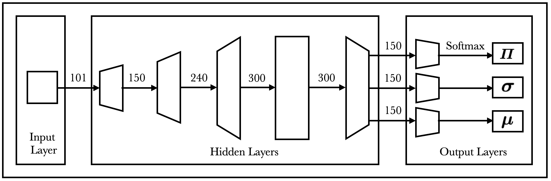
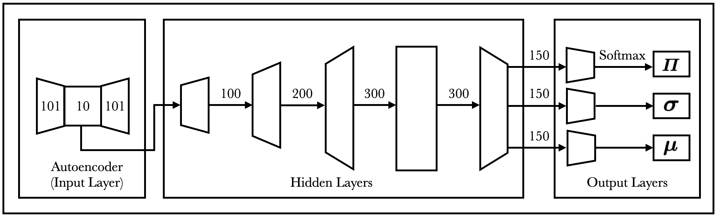
Figure 1: MDN structure without and with an autoencoder.

The structure of an MDN without (top) and with (bottom) an autoencoder (the numerical values in these figures are for illustration purposes) is shown in Fig. 1. The input data is a set of optical spectra discretized over the wavelength axis, and the hidden layers consist of fully-connected layers and activation functions. The first few hidden layers gradually expand the data size in order to allow the model to better capture the local patterns present in the input data. Once the size reaches the maximum, dropout is performed to improve the generalization ability of the model. After dropout, the data is downscaled to a reasonable size suitable for processing in the output layers. The output layers finally generate the key parameters $\Pi$, $\boldsymbol{\mu}$ and $\boldsymbol{\sigma}$ as the outputs of the MDN.

The loss function used in an MDN is the negative log likelihood (NLL) defined as:

$$-\log(\mathrm{p}(\mathbf{y}\mid\mathbf{x}))=-\log\left[\sum_{k}^{K}\Pi_{k}(\mathbf{x})\phi_{k}\left(\mathbf{y},\boldsymbol{\sigma}_{k}(\mathbf{x}),\boldsymbol{\mu}_{k}(\mathbf{x})\right)\right].$$ (3)

During model training in our numerical example, the NaN loss issue occurred frequently when the mixture component number $K$ was smaller than 5, possibly caused by the logarithm when being too close to zero or gradients become very small as they propagate through multiple layers. A method proposed in [17] was used to solve the NaN loss problem here, which addressed the issue by adding a small number like $10^{-5}$ in the logarithm, and the updated loss function is defined as follows:

$$-\log\left[\left(\sum_{k}^{K}\Pi_{k}(\mathbf{x})\phi_{k}\left(\mathbf{y},\boldsymbol{\sigma}_{k}(\mathbf{x})+10^{-5},\boldsymbol{\mu}_{k}(\mathbf{x})\right)\right)+10^{-5}\right].$$ (4)

2.3 Transfer Learning

An important challenge in MDN is selecting the proper number of mixture components $K$, to be set equal or larger than the number of possible solutions. However, this upper bound is typically unknown necessitating exploration of multiple different mixture component numbers. Also, another challenge of training an MDN is that the model parameters $\Pi$, $\boldsymbol{\mu}$ and $\boldsymbol{\sigma}$ must be jointly optimized, which can result computationally expensive. Moreover, optimizing all parameters simultaneously can be numerically unstable and can lead to degenerate predictions. Transfer learning offers a convenient way to address these issues.

The proposed transfer learning approach starts with $K=1$ to fully train the inverse model. Thereafter, model training with the next mixture component number reuses trained parameters, effectively shortening the training time. For the MDN models with different mixture component numbers, the hidden layers structure would still be the same and the only difference in model structure is the output layers. Therefore, the parameters of the hidden layers can be initialized with the hidden layers parameters of the previous model. As for the parameters initialization in the output layers, we propose two different methods.

The inverse model consists of three main outputs quantities, corresponding to $\boldsymbol{\Pi}$, $\boldsymbol{\mu}$ and $\boldsymbol{\sigma}$, respectively. Based on the structure of the loss function, the $\boldsymbol{\Pi}$ coefficient form a key factor in enabling the model to learn. In order to retain all the trained pdfs from the previous model, and provide the newly added distribution equal opportunities to learn during the new round of training, the $\Pi_{k}$ terms should be set to be equal. Due to the nature of the softmax function used in the output layer of $\boldsymbol{\Pi}$, simply initializing all the parameters for $\boldsymbol{\Pi}$ to be zero can achieve this goal, since this provides $\Pi_{k}=1/K$. As for the output layers of $\boldsymbol{\sigma}$ and $\boldsymbol{\mu}$, two initialization schemes are proposed. In the first approach, the first $K-1$ distributions inherit the parameters from the previous model, while the newly added distribution will randomly select the parameters of one distribution from the $K-1$ distributions as its parameters. In the second approach, the first $K-1$ distributions also inherit the same parameters as the previous model, but the new distribution uses the parameters corresponding to the distribution with the largest mixing coefficient in the previous model as its parameters instead of a random selection from the previous $K-1$ distributions. The first method is able to encourage the model to learn more diversified possible solutions with a randomness exploration characteristic. On the other hand, the second method can reduce the randomness in training, but may generally lead to a situation where most of the distributions are likely to be relatively similar to each other.

3 Numerical results

A grating-based multiband absorber is the device of interest in this example. It is a periodic structure with a unit cell composed of a five-layered metal-insulator-metal configuration as illustrated in Fig. 2. A periodic unit cell with an EM wave at normal incidence on top of the unit cell was simulated electromagnetically using a frequency-domain solver of COMSOL Multiphysics^®. The wavelength ($\lambda$) interval is in the visible range $[400-700]$ nm.

Figure 2: Cross-section of the unit cell.

The design parameters of the unit cell are: the unit cell period $p$, the width $w$ and the thicknesses $h_{1}$, $h_{2}$, $h_{3}$. The intervals of variation are [305-415] nm, [45-190] nm, [150-295] nm, [25-200] nm, and [80-165] nm, respectively. $101$ wavelength samples are chosen over the wavelength interval [400-700] nm. $3848$ scattered samples in the design space are chosen based on a Sobol quasi-random sequence scheme [18]. A possible fabrication constraint on the design parameters samples is considered, namely $p-w\geq 200$ nm, to ensure a certain space between unit cells. The EM absorbance response $A(p,w,h_{1},h_{2},h_{3},\lambda)$ of this device is considered in this example.

All model training and tests were performed on a MacOS 13.4.1 platform consisting of the Apple M1 CPU (8 processors) and 16 GB RAM. The code was implemented in PyTorch. The loss function used for the training is described in (4). The total number of spectra used in this work is 3848, and these spectra are divided into training, validation and test datasets according to the ratio $80\%-10\%-10\%$. Early stopping, a measure to avoid model overfitting, is used to optimize the training process. Table 1 provides information about the used model architecture ($K$ denotes the number of Gaussian pdfs and $5$ is the number of design parameters).

Table 1: MDN and AE models information.

# neurons (MDN)	$[101,150,240,300,300,150,[K,5K,5K]]$
# neurons (MDN+AE)	$[10,100,200,300,300,150,[K,5K,5K]]$
# neurons (AE)	$[101,128,256,512,256,10,256,512,256,128,101]$
Optimizer	Adam
Learning rate	$10^{-3}$
Activation functions	Sigmoid Linear Unit (SiLU)

A limit of 1000 epochs was set for training, subject to early-stopping. Table 2 summarizes the CPU time needed for the contructions of the MDNs ($K=1,...,10$) with and without autoencoder and with and without transfer learning approaches. TL1 and TL2 refer to the first and second proposed transfer learning strategies. Figs. 3-6 provide information about the accuracy of all these models considering training, validation, and test errors based on the NLL cost function in (4).

Table 2: CPU time comparison for the MDNs with and without autoencoder (AE) and transfer learning (TL)

No AE/TL	AE	TL1	AE+TL1	TL2	AE+TL2
$31\mathrm{~{}min}$	$28\mathrm{~{}min}$	$6\mathrm{~{}min}$	$10\mathrm{~{}min}$	$6\mathrm{~{}min}$	$10\mathrm{~{}min}$

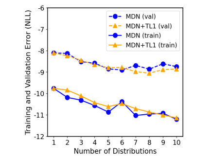
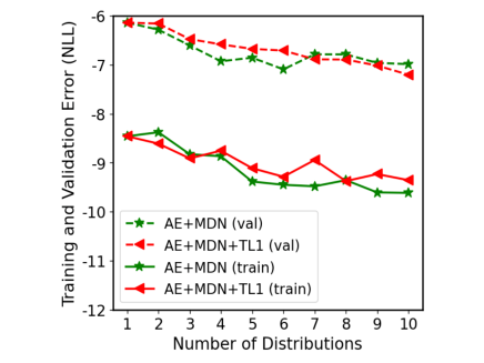
Figure 3: Training and validation loss of MDNs and AE+MDNs with and without transfer learning (TL1).

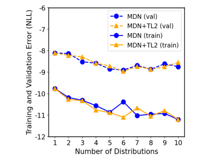
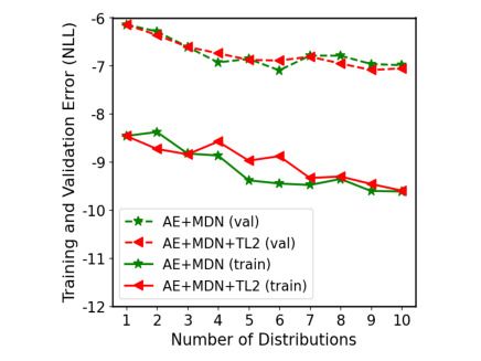
Figure 4: Training and validation loss of MDNs and AE+MDNs with and without transfer learning (TL2).

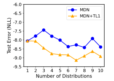
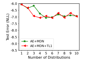
Figure 5: Test loss of MDNs and AE+MDNs with and without transfer learning (TL1).

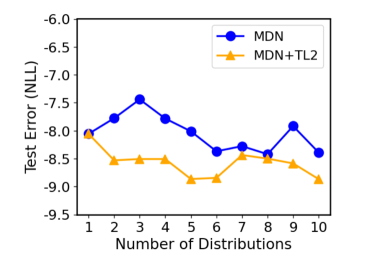
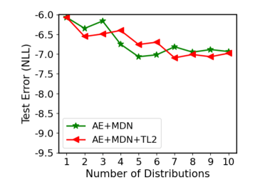
Figure 6: Test loss of MDNs and AE+MDNs with and without transfer learning (TL2).

These results show that the proposed transfer learning approaches work very well and allow reducing the training CPU time needed for multiple MDNs with a different number of Gaussian pdfs and even decreasing the test error. The autoencoder helps to reduce the training CPU time only when a transfer learning approach is not used, however there is a degradation in the accuracy performance of the MDNs overall.

We now illustrate additional results where $K=10$ for one sample of the test dataset in Figs. 7-10. For ease of visualization, we focus on the most significant $4$ solutions provided by the MDN without autoencoder and without transfer learning and the MDN without autoencoder and using the first transfer learning strategy. The vertical lines in Fig. 8 and Fig. 10 represent the exact values of the design parameters corresponding to the optical spectrum of the test sample. Looking at the absorbance plot, the blue line represents the test optical spectrum, while the red dashed line represents the spectrum computed by the EM solver using the optimal design parameters values predicted by the MDN. Sampling the output of the MDNs is not a task with a unique way of doing it. For the results shown here we have taken the mean values of the individual Gaussian pdfs composing the final pdf in (1). This is an approach but it is not the only one. Overall, MDNs provide probabilistic information that can be used to explore design solutions and as an initial solution generator for further optimization techniques. It can be noted that the MDN with transfer learning is more accurate than without transfer learning, and can well identify multiple design solutions. Fig. 11 shows the total pdf $\mathrm{p}(\mathbf{y}\mid\mathbf{x})$ (see (1)) for the two MDNs compared previously. Similarly, the vertical lines represent the exact values of the design parameters corresponding to the optical spectrum of the test sample.

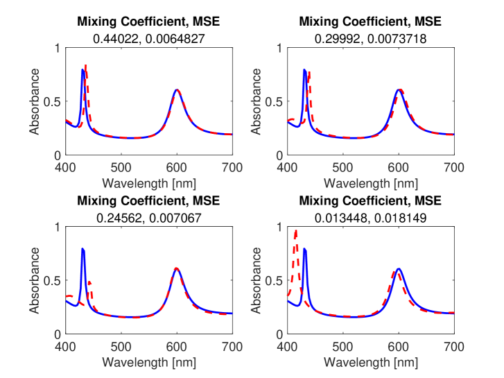
Figure 7: Prediction of the MDN model.

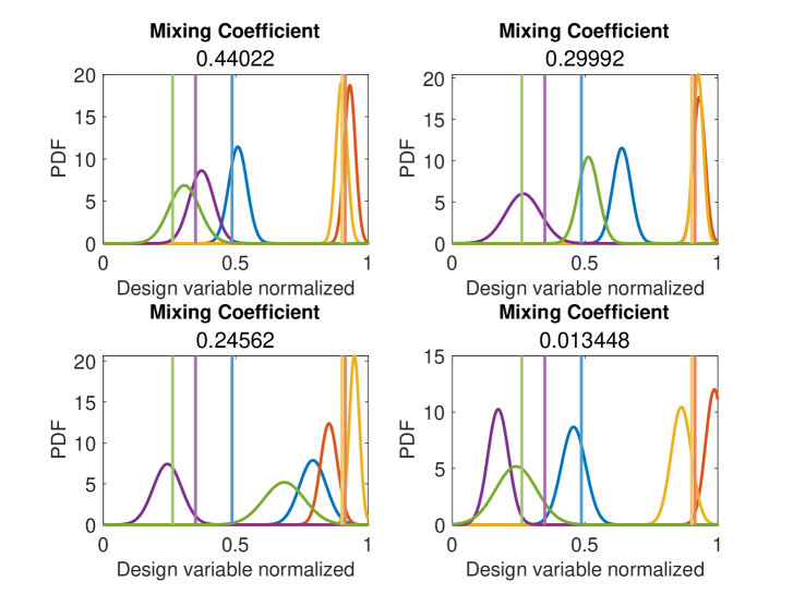
Figure 8: Gaussian pdfs of the MDN model.

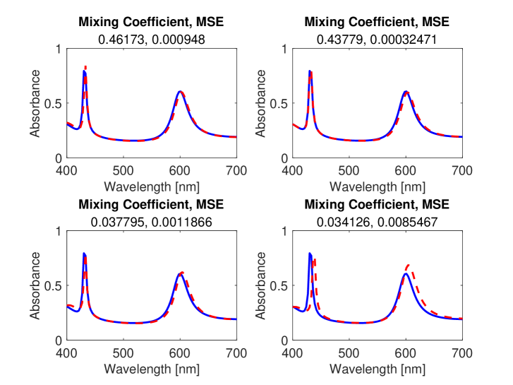
Figure 9: Prediction of the MDN+TL1 model.

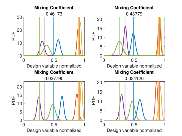
Figure 10: Gaussian pdfs of the MDN+TL1 model.

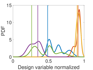
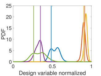
Figure 11: Total pdf $\mathrm{p}(\mathbf{y}\mid\mathbf{x})$ of the MDN (top) and MDN+TL1 (bottom) models.

4 Conclusion

This work presents a transfer-learning assisted MDN methodology for inverse modeling. This allows a rapid exploration of MDNs with different number of Gaussian distributions, while preserving a high accuracy in the prediction capability of the design solutions given an optical response as an input. Numerical results have validated the proposed techniques.

References

- [1] Wei Ma, Feng Cheng, and Yongmin Liu. Deep-learning-enabled on-demand design of chiral metamaterials. ACS Nano, 12(6):6326–6334, June 2018.
- [2] John Peurifoy, Yichen Shen, Li Jing, Yi Yang, Fidel Cano-Renteria, Brendan G. DeLacy, John D. Joannopoulos, Max Tegmark, and Marin Soljačić. Nanophotonic particle simulation and inverse design using artificial neural networks. Science Advances, 4(6):eaar4206, June 2018.
- [3] Dianjing Liu, Yixuan Tan, Erfan Khoram, and Zongfu Yu. Training deep neural networks for the inverse design of nanophotonic structures. ACS Photonics, 5(4):1365–1369, February 2018.
- [4] Rohit Unni, Kan Yao, and Yuebing Zheng. Deep convolutional mixture density network for inverse design of layered photonic structures. ACS Photonics, 7(10):2703–2712, 2020.
- [5] Peter R. Wiecha and Otto L. Muskens. Deep learning meets nanophotonics: A generalized accurate predictor for near fields and far fields of arbitrary 3d nanostructures. Nano Letters, 20(1):329–338, 2020.
- [6] Peter R. Wiecha, Arnaud Arbouet, Christian Girard, and Otto L. Muskens. Deep learning in nano-photonics: inverse design and beyond. Photon. Res., 9(5):B182–B200, May 2021.
- [7] Sunae So, Younghwan Yang, Taejun Lee, and Junsuk Rho. On-demand design of spectrally sensitive multiband absorbers using an artificial neural network. Photon. Res., 9(4):B153–B158, Apr 2021.
- [8] Nathan Bryn Roberts and Mehdi Keshavarz Hedayati. A deep learning approach to the forward prediction and inverse design of plasmonic metasurface structural color. Applied Physics Letters, 119(6):061101, 08 2021.
- [9] Rohit Unni, Kan Yao, Xizewen Han, Mingyuan Zhou, and Yuebing Zheng. A mixture-density-based tandem optimization network for on-demand inverse design of thin-film high reflectors. Nanophotonics, 10(16):4057–4065, October 2021.
- [10] Keisuke Kojima, Mohammad H. Tahersima, Toshiaki Koike-Akino, Devesh K. Jha, Yingheng Tang, Ye Wang, and Kieran Parsons. Deep neural networks for inverse design of nanophotonic devices. Journal of Lightwave Technology, 39(4):1010–1019, 2021.
- [11] Xiaopeng Xu, Chonglei Sun, Yu Li, Jia Zhao, Junlei Han, and Weiping Huang. An improved tandem neural network for the inverse design of nanophotonics devices. Optics Communications, 481:126513, 2021.
- [12] Clément Majorel, Christian Girard, Arnaud Arbouet, Otto L. Muskens, and Peter R. Wiecha. Deep learning enabled strategies for modeling of complex aperiodic plasmonic metasurfaces of arbitrary size. ACS Photonics, 9(2):575–585, 2022.
- [13] Francesco Ferranti. Feature-based machine learning for the efficient design of nanophotonic structures. Photonics and Nanostructures - Fundamentals and Applications, 52:101077, 2022.
- [14] Yang Deng, Simiao Ren, Jordan Malof, and Willie J. Padilla. Deep inverse photonic design: A tutorial. Photonics and Nanostructures - Fundamentals and Applications, 52:101070, 2022.
- [15] Omer Yesilyurt, Samuel Peana, Vahagn Mkhitaryan, Karthik Pagadala, Vladimir M. Shalaev, Alexander V. Kildishev, and Alexandra Boltasseva. Fabrication-conscious neural network based inverse design of single-material variable-index multilayer films. Nanophotonics, 12(5):993–1006, 2023.
- [16] Alexander Luce, Ali Mahdavi, Heribert Wankerl, and Florian Marquardt. Investigation of inverse design of multilayer thin-films with conditional invertible neural networks. Machine Learning: Science and Technology, 4(1):015014, February 2023.
- [17] Wei She, Renzhong Zhang, Wei Liu, Lihong Zhong, Bin Chen, and Zhao Tian. Mixture density network based on truncated distribution and genetic algorithm for wind power forecasting. Journal of Physics: Conference Series, 2409, 2022.
- [18] P. Brandimarte. Low-Discrepancy Sequences, pages 379–401. John Wiley and Sons, Inc., 2014.