A two-circuit approach to reducing quantum resources for
the quantum lattice Boltzmann method

Abstract

Computational fluid dynamics (CFD) simulations often entail a large computational burden on classical computers. At present, these simulations can require up to trillions of grid points and millions of time steps. To reduce costs, novel architectures like quantum computers may be intrinsically more efficient at the appropriate computation. Current quantum algorithms for solving CFD problems use a single quantum circuit and, in some cases, lattice-based methods. We introduce the a novel multiple circuits algorithm that makes use of a quantum lattice Boltzmann method (QLBM). The two-circuit algorithm we form solves the Navier–Stokes equations with a marked reduction in CNOT gates compared to existing QLBM circuits. The problem is cast as a stream function–vorticity formulation of the 2D Navier–Stokes equations and verified and tested on a 2D lid-driven cavity flow. We show that using separate circuits for the stream function and vorticity lead to a marked CNOT reduction: 35% in total CNOT count and 16% in combined gate depth. This strategy has the additional benefit of the circuits being able to run concurrently, further halving the seen gate depth. This work is intended as a step towards practical quantum circuits for solving differential equation-based problems of scientific interest.

I Introduction

Quantum computers can achieve complexity improvements by leveraging quantum mechanics principles such as superposition and entanglement. One example of quantum computing overcoming the limitations of computation on classical computers is Shor’s algorithm [1], which computes the prime factorization of integers in logarithmic time, providing an exponential speedup. Efforts are being made to explore the possibility of using quantum resources to speed up other important tasks. Example tasks include linear systems solvers [2, 3], Monte Carlo methods [4], and machine learning algorithms [5, 6]. With the recent progress of quantum hardware, various quantum algorithms have been purposed and examined for optimization problems [7], quantum chemistry [8], and finance [9].

An emerging use case of quantum computers is solving computational fluid dynamics (CFD) problems [10, 11, 12, 13, 14, 15, 16, 17, 18, 19, 20, 21, 22, 23, 24]. For example, some techniques for solving the incompressible Navier–Stokes equations rely on an efficient on a sparse linear solver. The Harrow–Hassidim–Lloyd (HHL) algorithm [2] promises an exponential speedup on such tasks, assuming the state preparation process and information readout are efficient. Lapworth [25] proposes a hybrid CFD solver based on the SIMPLE (Semi-Implicit Method for Pressure Linked Equations) algorithm and HHL. However, the number of operations HHL requires exceeds current quantum hardware capability. Instead, more proposals focus on using variational quantum algorithms (VQA) as near-term replacements for HHL to solve linear systems without any guaranteed complexity advantage. Demirdjian et al. [26] solves 1D advection-diffusion equation with Carleman linearization technique and variational quantum linear solver [27].

Mesoscale methods for solving the Navier–Stokes equations operate above the molecular level but below the continuum scale. These methods provide indirect solutions by solving the Boltzmann equation, which characterizes the statistical behavior of a system of particles. Two methods that can solve the Boltzmann equation are lattice gas automata [28, 29] and the lattice Boltzmann method (LBM) [30, 31]. Traditional LBM algorithms are suited for classical algorithms, though some algorithms for quantum devices have been developed. For example, previous art developed quantum algorithms for the lattice gas [32, 33, 34]. Itani and Succi [35] demonstrate a Carleman linearization for the collision term and further work in Itani et al. [36] shows unitary evolution for both collision and streaming operators. Further works have pushed these methods forward [37, 38].

Budinski [39] introduced a quantum lattice Boltzmann method (QLBM) for the advection–diffusion equation. This method simulates particles across a grid of lattice sites and extracts macroscopic quantities from mesoscopic simulations. Budinski [40] adapted the quantum circuit approximation to the Navier–Stokes equations. Using the stream function–vorticity formulation of the Navier–Stokes equations, the pressure term is removed, and the problem is reduced to an advection–diffusion equation and a Poisson equation. The strategy of these works involves a single quantum circuit for both equations.

This work formulates a two-circuit 2D QLBM to solve the incompressible Navier-Stokes equations. The method is validated against the classical LBM solution to the 2D lid-driven cavity flow problem. The quantum resources required for this QLBM approach are compared to other approaches. Section II describes the classical LBM theory for simulating the advection–diffusion equation. Section III.1 shows a single-circuit quantum implementation of the LBM for solving the advection–diffusion equation. In section IV, a description of the stream function-vorticity formulation of the Navier–Stokes equations and work on a two-circuit quantum implementation for solving the 2D Navier–Stokes equations are provided. Section V presents verification against the classically-solved LBM simulation for the lid-driven cavity problem and quantum resource estimation. Section VI serves to clarify the contributions of the method presented in this manuscript and its limitations.

II Classical lattice Boltzmann method

The LBM uses a grid of cells (shown in fig. 1) that contain particle distributions. The particles move into neighbor cells during each time step according to the Boltzmann equation [41, 42]:

$$f_{\alpha}(\bm{r}+e_{\alpha}\Delta t,t+\Delta t)=(1-\epsilon)f_{\alpha}(\bm{r},t)+\epsilon f_{\alpha}^{\text{(eq)}}+\Delta w_{\alpha}S,$$ (1)

where $e_{\alpha}$ is the velocity of a particle in link $\alpha$, $f_{\alpha}$ is the particle distribution along each $\alpha$, $t$ is time, $\bm{r}$ is the cell position, $S$ is the source term, $w_{\alpha}$ is the proportion of particles streaming in link $\alpha$, and $\epsilon=\Delta t/\tau$ where $\tau$ is a relaxation time. A D$n$Q$m$ scheme denotes an $n$-dimensional lattice grid with $m$ links, where a link is a direction in which particles can be propagated. The weights for the D2Q5 scheme (a 2D grid with 5 links per cell) are $w_{0}=2/6$ and $w_{2,3,4}=1/6$ following the directions shown in fig. 1 [43].

Figure 1: Illustration of a D2Q5 LBM lattice with a streaming particle and link weights $w_{\alpha}$.

We apply a new formulation to two PDE problems, the advection–diffusion and incompressible Navier–Stokes equations. Using the stream function–vorticity formulation, the Navier–Stokes equations reduce into two equations that closely resemble the advection–diffusion equation, so the latter will be examined first.

The advection–diffusion is

$$\frac{\partial\phi}{\partial t}+c\frac{\partial\phi}{\partial x}=D\frac{\partial^{2}\phi}{\partial x^{2}},$$ (2)

which represents advection as $c({\partial\phi}/{\partial x})$ and diffusion as $D({\partial^{2}\phi}/{\partial x^{2}})$. Here, $c$ and $D$ are advection and diffusion coefficients and $\phi(t,x)$ is a scalar concentration field.

For the advection–diffusion equation of (2), the equilibrium distribution function is

$$f_{\alpha}^{\text{(eq)}}(\bm{r},t)=w_{\alpha}\phi(\bm{r},t)\left(1+\frac{\bm{e_{\alpha}}\cdot\bm{c}}{c_{s}^{2}}\right),$$ (3)

where $\phi(\bm{r},t)$ corresponds to the lattice site at lattice position $\bm{r}$ = $(x_{i},y_{j})$, $\bm{c}$ is the advection velocity vector, and $c_{s}=1/\sqrt{3}$ is the speed of sound for the D2Q5 scheme [44]. The notation $x_{i}$ and $y_{j}$ denotes the $i$-th cell in the $x$ direction and the $j$-th cell in the $y$ coordinate direction.

Following standard practice [30], the relaxation time $\tau$ relates to the diffusion constant $D$ with

$$D=c_{s}^{2}\left(\tau-\frac{\Delta t}{2}\right).$$ (4)

Herein we use $D=1/6$, $c_{s}=1/\sqrt{3}$, and $\tau=\Delta t$. This gives $\varepsilon=\tau/\Delta t=1$ and

$$f_{\alpha}(\bm{r}+\bm{e_{\alpha}}\Delta t,t+\Delta t)=f_{\alpha}^{\text{(eq)}}$$ (5)

simplifies as

$$f_{\alpha}(\bm{r}+\bm{e_{\alpha}}\Delta t,t+\Delta t)=w_{\alpha}\phi(\bm{r},t)\left(1+\frac{\bm{e_{\alpha}}\cdot\bm{c}}{c_{s}^{2}}\right),$$ (6)

which includes the collision (3) and the streaming steps (5). The concentration field is thus

$$\phi(\bm{r},t)=\sum_{\alpha=0}^{N-1}f_{\alpha}(\bm{r},t),$$ (7)

summing the particle distributions across all link directions $\alpha$.

III Quantum lattice Boltzmann method

III.1 Advection–diffusion equation

A quantum circuit can implement the lattice Boltzmann method, which involves a similar approach to classical computation. Specifically, the quantum circuit performs the collision operator followed by the streaming of particles and subsequent recalculation of macroscopic variables. Boundary conditions are applied at the end of each time step. No special care is needed when boundary conditions are periodic; the left and right shift gates $R$ and $L$ automatically propagate boundary conditions to the designated lattice site for each link $\alpha$.

It is important to note that encoding input is a bottleneck in the algorithm. For the current study, the amplitude encoding technique described in the work of Shende et al. [45] is employed. Amplitude encoding is part of the Qiskit toolkit [46], though it is also a generic encoding algorithm with an expensive gate count.

We organize the quantum circuit for the advection–diffusion equation using a D2Q5 scheme with qubits organized into 4 registers, which are groupings of qubits. Registers $r_{0}$ and $r_{1}$ contain $\log M$ qubits, where $M$ is the number of lattice sites in each dimension. Register $d$ has $\lceil\log_{2}Q\rceil$ qubits, where $Q$ is the number of LBM links $\alpha$. Register $a$ holds a single ancilla qubit necessary for applying a non-unitary collision operator.

III.1.1 Encoding input

At the start of each time step, given a distribution $\phi(\bm{r},t)$, define $\phi(\alpha,\bm{r})$ to be the value of $\phi$ at time $t$ and position $\bm{r}$ at link direction $\alpha$. Given a discretized concentration

$$\phi(\alpha,\bm{r})=[\phi(0,0),\phi(0,1),\phi(0,2),\dots,\phi(4,M-2),\phi(4,M-1),\phi(4,M)],$$ (8)

the initial statevector $\ket{\psi_{0}}$ is

$$\ket{\psi_{0}}=\ket{0}_{a}\otimes\frac{1}{||\phi||}\sum_{i=0}^{2M-1}\phi(\alpha,\bm{r})\ket{i}.$$ (9)

This normalizes $\phi(\alpha,\bm{r})$, and the initial qubit states follow from amplitude encoding. In fig. 2, register $r_{0}$ stores the data at each link direction $\alpha$, and it can be retrieved by specifying the link $\alpha$ in register $d$.

Applying the collision operator to the initial statevector $\ket{\psi_{0}}$ is equivalent to multiplying the $\phi(\alpha,\bm{r})$ with weight coefficients

$$w_{\alpha}\left(1+\frac{\bm{e_{\alpha}}\cdot\bm{c}}{c_{s}^{2}}\right),$$ (10)

which follow from (3). This strategy is discussed further in the next subsection.

III.1.2 Collision operator

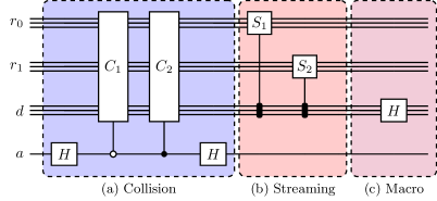
Figure 2: QLBM circuit for an advection–diffusion time step. The collision operator $A=(C_{1}+C_{2})/2$, and shift operators $R$, $L$, $D$, and $U$ propagate particles in each link direction $\alpha$. In panel (c), a Hadamard [47] gate is applied to the qubits in register $d$.

The collision step (fig. 2 (a)) computes the equilibrium distribution function $f_{a}^{\text{(eq)}}$, which requires computing the proportion of the distribution $\phi$ in each link $\alpha$. The collision operator entails applying the coefficient matrix $A$ to the current statevector $|\psi_{0}\rangle$.

The coefficient matrix $A$ is not unitary, so it cannot be directly translated into a quantum gate. An important strategy was described by Budinski [40]: A linear combination of unitary matrices split $A$ into two matrices $C_{1}$ and $C_{2}$, related to the original matrix as

$$C_{1,2}=A\pm i\sqrt{I-A^{2}}.$$ (11)

As $A=(C_{1}+C_{2})/2$, an operation with $A$ is computed via block encoding [48, 49], where $C_{1}$ and $C_{2}$ are unitary, but $A$ is, in general, not.

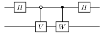
Figure 3: A block encoding of $B$ = $(V+W)/2$. Here, $V$ and $W$ are unitary matrices.

The circuit of fig. 3 evolves an input statevector $\ket{\psi}$ according to the unitary

$$U=\frac{1}{2}\begin{bmatrix}V+W&V-W\\ V-W&V+W\end{bmatrix},$$ (12)

where $B=(V+W)/2$. Thus, $B$ is a subblock of the block matrix $U$.

Post-selection selects quantum states for specific measurement outcomes. Here, we use post-selection to measure the result after the collision operator for a $0$ ancilla (after the block encoding).

The collision matrix is

$$A=\begin{bmatrix}k_{1}I_{n}&0\\ 0&k_{2}I_{n}\end{bmatrix},\quad\text{where}\quad k_{\alpha}=w_{\alpha}\left(1+\frac{\bm{e_{\alpha}}\cdot\bm{c}}{c_{s}^{2}}\right)$$ (13)

are the link coefficients described by (10). Panel (a) of fig. 2 uses a linear combination of unitaries to apply matrix $A$ to the input. The Hadamard gates are used for the block encoding process along with $C_{1}$ and $C_{2}$ operations, which are derived from the unitary matrices of (11). The coefficients representing the proportion of particles in each link $\alpha$ are $k_{1}$ and $k_{2}$. The collision matrices are

$$C_{1,2}=\begin{bmatrix}\exp(\pm i\cos^{-1}(k_{1}))I_{n}&0\\ 0&\exp(\pm i\cos^{-1}(k_{2}))I_{n}\end{bmatrix}.$$ (14)

The collision operator $A$ transforms statevector $\ket{\psi_{0}}$ via a linear combination of $C_{1}$ and $C_{2}$, but requires an ancilla qubit $a$, which stores orthogonal data $(C_{1}-C_{2})/2$ where the ancilla is $\ket{1}$. The orthogonal data was ignored through post-selection. The result of this linear combination is

$$\ket{\psi_{1}}=\frac{1}{||\phi||}\sum_{i}a_{i,i}\phi_{i,i}\ket{i},$$ (15)

which encodes the post-collision values for each link direction $\alpha$, for which the ancilla is $\ket{0}$.

III.2 Particle streaming

The streaming step propagates particles in each link $\alpha$ to the neighboring site. Figure 5 shows the shift operators $R_{n}$ and $L_{n}$, which are controlled on link qubits $d$ and stream particles to neighboring lattice sites. The shift matrices are permutation matrices as

$$R_{n}=\begin{bmatrix}0&0&\cdots&0&1\\ 1&0&\cdots&0&0\\ 0&1&\cdots&0&0\\ \vdots&\vdots&\ddots&\vdots&\vdots\\ 0&0&\cdots&1&0\end{bmatrix}\quad\text{and}\quad L_{n}=\begin{bmatrix}0&1&\cdots&0&0\\ \vdots&\vdots&\ddots&\vdots&\vdots\\ 0&0&\cdots&1&0\\ 0&0&\cdots&0&1\\ 1&0&\cdots&0&0\end{bmatrix},$$ (16)

and are both unitary matrices.

The resulting statevector $\ket{\psi_{2}}$ has a distribution shifted to a neighbor lattice site corresponding to its link value $\alpha_{i}$. The right and left shift gates $R$ and $L$, shown in fig. 4, are controlled on the link qubits $d$ to act on the part of the statevector corresponding to a distribution $\alpha$. Figure 5 shows the up and down operators $U$ and $D$, which are implemented via the $L$ and $R$ operators applied via $r_{1}$.

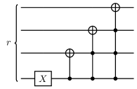
(a) Left shift operator $L$.

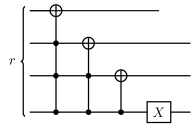
(b) Right shift operator $R$.

Figure 4: Circuit decomposition for (a) left shift and (b) right shift operators. These gates are applied to qubits in $r_{1}$ for left and right shifts and qubits in $r_{2}$ for up- and down-shifts.

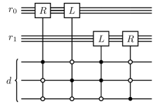
Figure 5: Streaming for a two-dimensional lattice grid. The streaming step uses right and left shift operators $R$ and $L$ to shift distributions in their respective link directions $\alpha_{1}$ and $\alpha_{2}$ by controlling the gates on qubits in each link register $d$.

III.3 Macroscopic variable retrieval

We retrieve the distribution $\phi(\bm{r},t)$ by summing $f_{\alpha}^{\mathrm{(eq)}}$ over the link directions $\alpha$. In terms of quantum operations, this is accomplished via the application of Hadamard gates to each of the qubits in link registers $d$, as shown in fig. 2 (c) [47]. A Hadamard gate $H$ applied to a statevector $\ket{\psi}$, resulting in

$$H|\psi\rangle=\frac{1}{\sqrt{2}}\begin{bmatrix}1&1\\ 1&-1\end{bmatrix}\begin{bmatrix}a\\ b\end{bmatrix}=\frac{1}{\sqrt{2}}\begin{bmatrix}a+b\\ a-b\end{bmatrix}=\frac{a+b}{\sqrt{2}}|0\rangle+\frac{a-b}{\sqrt{2}}|1\rangle.$$ (17)

Thus, when the Hadamard gate is applied to a link qubit in $d$, it stores the sum of the two amplitudes as the $\ket{0}$ amplitude and the difference as the $\ket{1}$ amplitude. So, the sum can be post-selected by ignoring $\ket{1}$ measurements. This means that the Hadamard gates will sum the distributions but introduce a factor of $1/\sqrt{2}$ per gate. This prefactor is post-processed out of the computation by multiplication of a factor of $\sqrt{2}^{\log Q}$ where $Q=|\alpha|$ is the number of link distributions. At each time step, we retrieve the circuit result via state tomography, which must be used to extract the first $M$ lattice site elements.

IV Quantum lattice Boltzmann method for the Navier–Stokes Equations

IV.1 Stream function–vorticity formulation

The incompressible 2D Navier–Stokes equations in Cartesian coordinates are

$$\frac{\partial u}{\partial t}+u\frac{\partial u}{\partial x}+v\frac{\partial u}{\partial y} =-\frac{\partial p}{\partial x}+\frac{1}{\mbox{\text{Re}}}\left(\frac{\partial^{2}u}{\partial x^{2}}+\frac{\partial^{2}u}{\partial y^{2}}\right),$$ (18)

$$\frac{\partial v}{\partial t}+u\frac{\partial v}{\partial x}+v\frac{\partial v}{\partial y} =-\frac{\partial p}{\partial y}+\frac{1}{\mbox{\text{Re}}}\left(\frac{\partial^{2}v}{\partial x^{2}}+\frac{\partial^{2}v}{\partial y^{2}}\right),$$ (19)

where $u$ and $v$ are the velocity components in the $x$ and $y$ coordinate directions, $p$ is the pressure, and Re is the Reynolds number, which is the ratio of inertial to viscous effects [50].

Taking the curl of the above Navier–Stokes equations recasts them in the so-called vorticity–stream function formulation, removing the pressure term $p$ and yielding

$$\frac{\partial^{2}\psi}{\partial x^{2}}+\frac{\partial^{2}\psi}{\partial y^{2}} =-\omega,$$ (20)

$$\frac{\partial\omega}{\partial t}+u\frac{\partial\omega}{\partial x}+v\frac{\partial\omega}{\partial y} =\frac{1}{\mbox{\text{Re}}}\left(\frac{\partial^{2}\omega}{\partial x^{2}}+\frac{\partial^{2}\omega}{\partial y^{2}}\right).$$ (21)

In this formulation, (20) and (21) use vorticity $\omega$ and stream function $\psi$ instead of directional speeds $u$ and $v$. The velocity vector is thus $\bm{u}=\{u,v\}$. The stream function relates to the directional velocities as

$$\frac{\partial\psi}{\partial x}=u\quad\text{and}\quad\frac{\partial\psi}{\partial y}=-v.$$ (22)

So, (20) is a Poisson equation in stream function $\phi$ and (21) is a advection–diffusion equation in vorticity $\omega$.

IV.1.1 Lattice-based representation

With the stream function–vorticity formulation, the collision, streaming, and macro lattice stages follow as

$$f_{\alpha}^{\text{(eq)}}(\bm{r},t) =w_{\alpha}\omega(\bm{r},t)\left(1+\frac{\bm{e}_{\alpha}\cdot\bm{u}}{c_{s}^{2}}\right),$$ (23)

$$f_{\alpha}(\bm{r}+\bm{e}_{\alpha}\Delta t,t+\Delta t) =f_{\alpha}^{\text{(eq)}},$$ (24)

$$\omega(\bm{r},t) =\sum_{\alpha}f_{\alpha}(\bm{r},t),$$ (25)

respectively. These stages, buttressed via the circuits of section III.1, enable the vorticity $\omega$ computation.

The equilibrium distribution function for the Poisson equation ($\nabla^{2}\psi=-\omega$) is $g_{\alpha}^{\text{(eq)}}(\bm{r},t)=w_{\alpha}\psi(\bm{r},t)$. The streaming and macro steps match those of section III.2 and section III.3, but the source term $S=-\omega$ is added during the collision step (a). Thus, the relaxation operator is

$$g_{\alpha}(\bm{r}+\bm{e}_{\alpha}\Delta t,t+\Delta t)=g_{\alpha}^{\text{(eq)}}+\Delta w_{\alpha}S,$$ (26)

and macro retrieval equation

$$\psi(\bm{r},t)=\sum_{\alpha}g_{\alpha}(\bm{r},t).$$ (27)

IV.1.2 Boundary conditions

The validation problem for the proposed method is a 2D lid-driven cavity flow. The spatial domain is $\Omega\in x,y$ with lengths $L_{x}$ and $L_{y}$ and boundary $\partial\Omega$. The stream function $\psi$ is constant along the boundaries, with $\psi=0$ used here. For the lattice Boltzmann method,

$$\psi=\sum_{\alpha=0}^{N_{l}-1}g_{\alpha}^{\text{(eq)}}=g_{0}+g_{1}+g_{2}+g_{3}+g_{4},\quad\text{so,}\quad g_{\partial\Omega}=-\sum_{\alpha|\alpha\neq\partial\Omega}g_{\alpha}.$$ (28)

Defining the vorticity expression (20) in terms of the stream function and expanding it in its Taylor series gives

$$\omega_{i,N}=-2\left(\frac{\psi}{\Delta y^{2}}+\frac{U}{\Delta y}\right),$$ (29)

along the boundaries $\partial\Omega$, where $U$ is wall-parallel velocity of the top wall. For a stationary wall, $U=0$. The wall equilibrium distribution in the direction of the wall is

$$g(x,y)_{\partial\Omega}=-{\sum_{\alpha|\alpha\neq\partial\Omega}g_{\alpha}}-2\left(\frac{-\psi}{\Delta y^{2}}+\frac{U}{\Delta y}\right).$$ (30)

To implement (30), the matrix

$$B=\begin{bmatrix}0&\cdots&0\\ \vdots&I_{N-2}&\vdots\\ 0&\cdots&0\end{bmatrix}$$ (31)

is applied to the statevector $|\phi\rangle$, where $B$ is of size $N\times N$, where $N=\log(n)$ in each dimension and $I_{n}$ denotes the size $n$ identity matrix. So, $g_{\partial\Omega}=0$, while retaining other distribution values, enforces the boundary condition for the stream function circuit $|\psi_{\text{b.c.}}\rangle=|0\rangle^{\otimes n}$.

Due to its non-unitary properties, the vorticity circuit boundary conditions are applied via a linear combination of $B$. This linear unitary combination is

$$D_{1,2}=B\pm i\sqrt{I_{N}-B^{2}},$$ (32)

following section III.1.2.

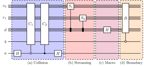
Figure 6: A D2Q5 vorticity circuit, including boundary conditions. Compared with the advection–diffusion circuit in fig. 2, this has an additional qubit $b$ required to hold boundary conditions and an additional operation required to compute them. However, if boundary conditions are computed classically, the vorticity and advection–diffusion circuits are identical.

IV.2 Quantum circuits

IV.2.1 Vorticity circuit

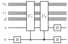
Figure 7: Collision portion of the stream function circuit. An additional qubit $s$ stores the source term, and an additional Hadamard gate on qubit s after the block encoding adds the source term to the link distributions $\alpha_{i}$ before streaming.

The vorticity circuit computes the vorticity $\omega$ for the current time step. Note the vorticity circuit in fig. 6 and advection–diffusion circuit in fig. 2 match, except for boundary conditions. This occurs because the vorticity equation (described in eq. 21) follows the same form as the diffusion equation. The Navier–Stokes algorithm’s vorticity circuit is identical to the advection–diffusion circuit for classically-computed boundary conditions.

If boundary conditions are included, an extra qubit $b$ stores them. Boundary conditions require additional computation, as enforcing such conditions is not a unitary operation. For this, the linear combination of unitaries is used [51], described further in section III.1.2, The input to this circuit for the no-boundary version is the previous time step’s vorticity $\omega_{t-1}$. When using boundary conditions, the circuit input includes pre-computed boundary conditions in the boundary qubit $b$, computed following the descriptions in section IV.1.2.

IV.2.2 Stream function circuit

The stream function circuit is the other quantum circuit used in this two-circuit model. The D2Q5 stream function circuit shown in fig. 7 is referred to for additional context. This circuit is similar in character to the advection–diffusion circuit with classical boundary conditions but an additional source. A key difference is the requirement of an extra qubit $s$ to store the source term, $S=-\omega$, as shown in fig. 7.

The $C_{1}$ and $C_{2}$ gates also operate on the source term, and the Hadamard gate on qubit $s$ adds this source to the equilibrium stream function distribution function $g_{\alpha}^{\mathrm{(eq)}}$. The same qubit-addition process from section IV.2.1 applies. Boundary conditions require an additional $b$ qubit store and a boundary gate $B$, which is not unitary and again is implemented via a linear combination of matrices following (12). The previous stream function, $\psi_{t-1}$, and source term, $S=-\omega_{t-1}$, serve as the input to the stream function circuit. The boundary conditions are computed according to section IV.1.2 for our quantum boundary condition variant.

V Simulations and results

V.1 Advection–diffusion equation

Example results for the QLBM circuit applied to the advection–diffusion equation are shown for two exemplar cases. In the 1D case, D1Q2 and D1Q3 lattice schemes simulate a dense concentration of $\rho=0.2$ at source $x_{i}=10$ undergoing advection and diffusion with uniform advection velocity of $c=1/5$ and diffusion coefficient $D=1/6$. The validation problem for the 2D case follows a diffusing concentration $\rho=0.3$ at source $(x_{i},y_{j})=(4,4)$ and $0.1$ elsewhere, solved via a D2Q5 scheme.

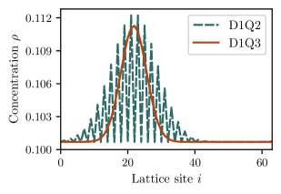
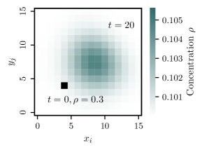
(a) D1Q2 and D1Q3	(b) D2Q5

Figure 8: Quantum LBM (a) D1Q2, D1Q3, and (b) D2Q5 results to the advection–diffusion equation. The initial condition in (a) is a point source of $\rho=0.2$ at $x=10$ and $\rho=0.1$ in all other sites. The initial condition in (b) is a point source of $\rho=0.3$ at $(x,y)=(4,4)$ and $\rho=0.1$ elsewhere.

Figure 8 shows the results of these simulations, showing the checkerboard pattern that arises in D1Q2 due to the distribution moving wholly into neighboring areas, resulting in half of the lattice sites having zero particles. The algorithmic deficiency is remedied via the D1Q3 lattice scheme with an $w_{0}=2/3$ of the particles, which remain in their current lattice site. Figure 8 (a) shows that the D1Q2 and D1Q3 schemes return similar results, but D1Q3 resolves the checkerboarding problem.

Figure 8 (b) shows the results of the 2D test problem solved with the D2Q5 scheme. We observe a source with an advection velocity in the positive $x$ and $y$ directions, advecting in the direction of the velocity and diffusing outwards from an initial source at $(x_{i}=4,y_{j}=4)$. The solution behaves as expected and agrees with classical LBM results.

V.2 Navier–Stokes equations

Figure 9 shows isocontours of the stream function for a lid-driven cavity problem. The problem serves to verify the two-circuit QLBM against a classical implementation of the lattice Boltzmann method.

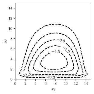
Figure 9: A 2D lid-driven cavity flow. Steady-state stream function isocontours are shown as labeled. The initial conditions are $\psi=0$, $w=0$, and $U=1$.

To define relative errors between the quantum and classical lattice algorithms, we denote

$$\psi_{i,j}=\psi_{(x_{i},y_{j})}\quad\text{and}\quad\omega_{i,j}=\omega_{(x_{i},y_{j})},$$ (33)

where $x_{i}=i\Delta x$ and $y_{j}=j\Delta y$. The local $L_{1}$ relative error between the classical and two-circuit QLBM Navier–Stokes solver is, thus,

$$\varepsilon_{\psi;i,j}=\frac{\psi_{i,j}^{\text{classic.}}-\psi_{i,j}^{\text{quant.}}}{\psi_{i,j}^{\text{classic.}}}\quad\text{and}\quad\varepsilon_{\omega;i,j}=\frac{\omega_{i,j}^{\text{classic.}}-\omega_{i,j}^{\text{quant.}}}{\omega_{i,j}^{\text{classic.}}}.$$ (34)

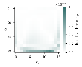
(a) Relative error $\varepsilon_{\omega}$ for vorticity circuit

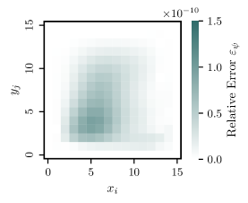
(b) Relative error $\varepsilon_{\psi}$ for stream function circuit

Figure 10: Relative error between the classical LBM and two-circuit quantum methods for (a) vorticity and (b) stream function.

The relative errors are shown for the cavity problem in fig. 10. The two-circuit QLBM has a close agreement with the results of the classical LBM when simulated with the statevector simulator in Qiskit’s SDK [46], as shown in fig. 10. The state vector simulator perfects exact tomography but is generally limited to relatively small simulations due to exponentially increasing memory requirements with qubit numbers.

V.2.1 Quantum resource estimation and improvement

	CNOT Gates	Circuit Depth
Single-circuit QLBM	25	58
Stream function	4.3	9.4
Vorticity	12	39
Stream function without boundaries	4.2	15
Vorticity without boundaries	3	6.5

Table 1: Quantum resource estimation (all counts are in units of $10^{4}$) for a D2Q5 algorithm with lattice size $64\times 64$.

Implementing the two-circuit method for solving the Navier–Stokes equations using quantum lattice-based algorithms shows quantum resource efficiency advantages over the single-circuit method. The difference in accuracy between the classical lattice Boltzmann method (LBM) and the two-circuit implementation is negligible. The stream function and vorticity circuits can be run concurrently for each time step, saving computational time. Other improvements include circuits with classical boundary conditions, decreasing circuit depth, and the number of CNOT gates compared to a single-circuit strategy. CNOT gates are slower than single qubit gates such as Hadamard gates, so CNOT gate count is used here to compare quantum resource costs.

The Qiskit transpiler translates the circuits of previous sections into single qubit and CNOT gates. The results of table 1 show that pre-computing the boundary conditions using classical methods reduces the gate count by at least $35\%$. Even when these circuits are computed in serial, the combined quantum resources for stream function and vorticity circuits remain notably lower than those of a single-circuit QLBM. Of course, parallel implementations are natural with the two-circuit approach.

VI Conclusion

This work presents improvements on the quantum lattice Boltzmann method for solving the two-dimensional Navier–Stokes equations. Testing on the validation problem shows that the error between the quantum and classical LBM methods is negligible. Runtime and quantum resources markedly decrease from a previous single-circuit implementation of an otherwise similar algorithm [40]. The number of qubits required scales as $O(\log M)$ where $M$ is the size of the grid, as opposed to the linear scaling of previous related works such as Yepez [34], which makes the prospect of near-term implementations on quantum hardware potentially viable, though not tested here.

The CNOT count of the vorticity and stream function circuits scales as $O(\alpha M)$. However, the encoding step is an efficiency bottleneck, occurring after each time step. Readout of the statevector and subsequent re-encoding decreases the efficiency of this method and is an important consideration for future work. Using the two-circuit quantum lattice Boltzmann method simplifies the quantum algorithm implementation and reduces the required quantum resources.

References

- Shor [1997] P. W. Shor, Polynomial-time algorithms for prime factorization and discrete logarithms on a quantum computer, SIAM Journal on Computing 26, 1484 (1997).
- Harrow et al. [2009] A. W. Harrow, A. Hassidim, and S. Lloyd, Quantum algorithm for solving linear systems of equations, Physical Review Letters 103, 150502 (2009).
- Clader et al. [2013] B. D. Clader, B. C. Jacobs, and C. R. Sprouse, Preconditioned quantum linear system algorithm, Physical Review Letters 110, 250504 (2013).
- Montanaro [2015] A. Montanaro, Quantum speedup of Monte Carlo methods, Proceedings of the Royal Society A: Mathematical, Physical and Engineering Sciences 471, 20150301 (2015).
- Havlíček et al. [2019] V. Havlíček, A. D. Córcoles, K. Temme, A. W. Harrow, A. Kandala, J. M. Chow, and J. M. Gambetta, Supervised learning with quantum-enhanced feature spaces, Nature 567, 209 (2019).
- Liu et al. [2021] Y. Liu, S. Arunachalam, and K. Temme, A rigorous and robust quantum speed-up in supervised machine learning, Nature Physics 17, 1013 (2021).
- Farhi et al. [2014] E. Farhi, J. Goldstone, and S. Gutmann, A quantum approximate optimization algorithm, arXiv preprint arXiv:1411.4028 (2014).
- Cao et al. [2019] Y. Cao, J. Romero, J. P. Olson, M. Degroote, P. D. Johnson, M. Kieferová, I. D. Kivlichan, T. Menke, B. Peropadre, N. P. D. Sawaya, S. Sim, L. Veis, and A. Aspuru-Guzik, Quantum chemistry in the age of quantum computing, Chemical Reviews 119, 10856 (2019).
- Herman et al. [2023] D. Herman, C. Googin, X. Liu, Y. Sun, A. Galda, I. Safro, M. Pistoia, and Y. Alexeev, Quantum computing for finance, Nature Reviews Physics 5, 450 (2023).
- Succi et al. [2023] S. Succi, W. Itani, K. Sreenivasan, and R. Steijl, Quantum computing for fluids: Where do we stand?, Europhysics Letters 144, 10001 (2023).
- Succi et al. [2024] S. Succi, W. Itani, C. Sanavio, K. R. Sreenivasan, and R. Steijl, Ensemble fluid simulations on quantum computers, Computers & Fluids 270, 106148 (2024).
- Steijl [2019] R. Steijl, Quantum algorithms for fluid simulations, Advances in Quantum Communication and Information , 31 (2019).
- Moawad et al. [2022] Y. Moawad, W. Vanderbauwhede, and R. Steijl, Investigating hardware acceleration for simulation of CFD quantum circuits, Frontiers in Mechanical Engineering 8, 925637 (2022).
- Steijl and Barakos [2018] R. Steijl and G. N. Barakos, Parallel evaluation of quantum algorithms for computational fluid dynamics, Computers & Fluids 173, 22 (2018).
- Gaitan [2020] F. Gaitan, Finding flows of a Navier–Stokes fluid through quantum computing, npj Quantum Information 6, 61 (2020).
- Bharadwaj and Sreenivasan [2020] S. S. Bharadwaj and K. R. Sreenivasan, Quantum computation of fluid dynamics, arXiv preprint arXiv:2007.09147 (2020).
- Bharadwaj and Sreenivasan [2023] S. S. Bharadwaj and K. R. Sreenivasan, Hybrid quantum algorithms for flow problems, Proceedings of the National Academy of Sciences 120, e2311014120 (2023).
- Li et al. [2023] X. Li, X. Yin, N. Wiebe, J. Chun, G. K. Schenter, M. S. Cheung, and J. Mülmenstädt, Potential quantum advantage for simulation of fluid dynamics, arXiv preprint arXiv:2303.16550 (2023).
- Oz et al. [2022] F. Oz, R. K. Vuppala, K. Kara, and F. Gaitan, Solving Burgers’ equation with quantum computing, Quantum Information Processing 21, 1 (2022).
- Jaksch et al. [2023] D. Jaksch, P. Givi, A. J. Daley, and T. Rung, Variational quantum algorithms for computational fluid dynamics, AIAA Journal 61, 1885 (2023).
- Givi et al. [2020] P. Givi, A. J. Daley, D. Mavriplis, and M. Malik, Quantum speedup for aeroscience and engineering, AIAA Journal 58, 3715 (2020).
- Xu et al. [2018] G. Xu, A. J. Daley, P. Givi, and R. D. Somma, Turbulent mixing simulation via a quantum algorithm, AIAA Journal 56, 687 (2018).
- Xu et al. [2019] G. Xu, A. J. Daley, P. Givi, and R. D. Somma, Quantum algorithm for the computation of the reactant conversion rate in homogeneous turbulence, Combustion Theory and Modelling 23, 1090 (2019).
- Sammak et al. [2015] S. Sammak, A. Nouri, N. Ansari, and P. Givi, Quantum computing and its potential for turbulence simulations, in Mathematical Modeling of Technological Processes: 8th International Conference, CITech 2015, Almaty, Kazakhstan, September 24-27, 2015, Proceedings 8 (Springer, 2015) pp. 124–132.
- Lapworth [2022] L. Lapworth, A hybrid quantum-classical CFD methodology with benchmark HHL solutions, arXiv preprint arXiv:2206.00419 (2022).
- Demirdjian et al. [2022] R. Demirdjian, D. Gunlycke, C. A. Reynolds, J. D. Doyle, and S. Tafur, Variational quantum solutions to the advection–diffusion equation for applications in fluid dynamics, Quantum Information Processing 21, 322 (2022).
- Bravo-Prieto et al. [2020] C. Bravo-Prieto, R. LaRose, M. Cerezo, Y. Subasi, L. Cincio, and P. J. Coles, Variational quantum linear solver, arXiv preprint arXiv:1909.05820 (2020).
- Frisch et al. [1986a] U. Frisch, D. d’Humieres, B. Hasslacher, P. Lallemand, Y. Pomeau, and J. P. Rivet, Lattice gas hydrodynamics in two and three dimensions, in Modern Approaches to Large Nonlinear Physical Systems Workshop (1986).
- Frisch et al. [1986b] U. Frisch, B. Hasslacher, and Y. Pomeau, Lattice-gas automata for the Navier–Stokes equation, Physical Review Letters 56, 1505 (1986b).
- Krüger et al. [2016] T. Krüger, H. Kusumaatmaja, A. Kuzmin, O. Shardt, G. Silva, and E. Viggen, The Lattice Boltzmann Method: Principles and Practice, Graduate Texts in Physics (Springer International Publishing, 2016).
- Chen and Doolen [1998] S. Chen and G. D. Doolen, Lattice Boltzmann method for fluid flows, Annual Review of Fluid Mechanics 30, 329 (1998).
- Yepez [1998] J. Yepez, Lattice-gas quantum computation, International Journal of Modern Physics C 09, 1587 (1998).
- Yepez [2001] J. Yepez, Quantum lattice-gas model for computational fluid dynamics, Physical Review E 63, 046702 (2001).
- Yepez [2002] J. Yepez, Quantum lattice-gas model for the Burgers equation, Journal of Statistical Physics 107, 203 (2002).
- Itani and Succi [2022] W. Itani and S. Succi, Analysis of Carleman linearization of lattice Boltzmann, Fluids 7 (2022).
- Itani et al. [2023] W. Itani, K. R. Sreenivasan, and S. Succi, Quantum algorithm for lattice Boltzmann (QALB) simulation of incompressible fluids with a nonlinear collision term, arXiv preprint arXiv:2304.05915 (2023).
- Sanavio and Succi [2023] C. Sanavio and S. Succi, Quantum lattice Boltzmann–Carleman algorithm, arXiv preprint arXiv:2310.17973 (2023).
- Todorova and Steijl [2020] B. N. Todorova and R. Steijl, Quantum algorithm for the collisionless Boltzmann equation, Journal of Computational Physics 409, 109347 (2020).
- Budinski [2021a] L. Budinski, Quantum algorithm for the advection–diffusion equation simulated with the lattice Boltzmann method, Quantum Information Processing 20, 57 (2021a).
- Budinski [2021b] L. Budinski, Quantum algorithm for the Navier–Stokes equations, arXiv preprint arXiv:2103.03804 (2021b).
- Rothman and Zaleski [1997] D. H. Rothman and S. Zaleski, Lattice-gas cellular automata: Simple models of complex hydrodynamics (Cambridge University Press, 1997).
- Rivet and Boon [2001] J.-P. Rivet and J. P. Boon, Lattice Gas Hydrodynamics (Cambridge University Press, 2001).
- Ginzburg [2005] I. Ginzburg, Equilibrium-type and link-type lattice Boltzmann models for generic advection and anisotropic-dispersion equation, Advances in Water Resources 28, 1171 (2005).
- Servan-Camas and Tsai [2009] B. Servan-Camas and F. T.-C. Tsai, Non-negativity and stability analyses of lattice boltzmann method for advection–diffusion equation, Journal of Computational Physics 228, 236 (2009).
- Shende et al. [2006] V. Shende, S. Bullock, and I. Markov, Synthesis of quantum-logic circuits, IEEE Transactions on Computer-Aided Design of Integrated Circuits and Systems 25, 1000 (2006).
- Qiskit Contributors [2023] Qiskit Contributors, Qiskit: An open-source framework for quantum computing (2023).
- Nielsen and Chuang [2000] M. A. Nielsen and I. L. Chuang, Quantum Computation and Quantum Information (Cambridge University Press, 2000).
- Chakraborty et al. [2019] S. Chakraborty, A. Gilyén, and S. Jeffery, The power of block-encoded matrix powers: Improved regression techniques via faster Hamiltonian simulation, arXiv preprint arXiv:1804.01973 (2019).
- Low and Chuang [2019] G. H. Low and I. L. Chuang, Hamiltonian simulation by qubitization, Quantum 3, 163 (2019).
- Batchelor [1967] G. K. Batchelor, An introduction to fluid dynamics (Cambridge University Press, 1967).
- Meyer [1997] D. A. Meyer, Quantum mechanics of lattice gas automata: One-particle plane waves and potentials, Physical Review E 55, 5261 (1997).