Constraint-Generation Policy Optimization (CGPO): Nonlinear Programming for Policy Optimization in Mixed Discrete-Continuous MDPs

Abstract

We propose Constraint-Generation Policy Optimization (CGPO) for optimizing policy parameters within compact and interpretable policy classes for mixed discrete-continuous Markov Decision Processes (DC-MDPs). CGPO is not only able to provide bounded policy error guarantees over an infinite range of initial states for many DC-MDPs with expressive nonlinear dynamics, but it can also provably derive optimal policies in cases where it terminates with zero error. Furthermore, CGPO can generate worst-case state trajectories to diagnose policy deficiencies and provide counterfactual explanations of optimal actions. To achieve such results, CGPO proposes a bi-level mixed-integer nonlinear optimization framework for optimizing policies within defined expressivity classes (i.e. piecewise (non)-linear) and reduces it to an optimal constraint generation methodology that adversarially generates worst-case state trajectories. Furthermore, leveraging modern nonlinear optimizers, CGPO can obtain solutions with bounded optimality gap guarantees. We handle stochastic transitions through explicit marginalization (where applicable) or chance-constraints, providing high-probability policy performance guarantees. We also present a road-map for understanding the computational complexities associated with different expressivity classes of policy, reward, and transition dynamics. We experimentally demonstrate the applicability of CGPO in diverse domains, including inventory control, management of a system of water reservoirs, and physics control. In summary, we provide a solution for deriving structured, compact, and explainable policies with bounded performance guarantees, enabling worst-case scenario generation and counterfactual policy diagnostics.

Introduction

An important aim of sequential decision optimization of challenging Discrete-Continuous Markov Decision Processes (DC-MDPs) in the artificial intelligence, operations research and control domains is to derive policies that achieve optimal control. A desirable property of such policies is compactness of representation, which provides efficient execution on resource-constrained systems such as mobile devices (Wang et al. 2022), as well as the potential for introspection and explanation (Topin et al. 2021). Moreover, while the derived policy is expected to perform well in expectation, in many applications it is desirable to obtain bounds on maximum policy error and and the scenarios that induce worst-case policy performance (Corso et al. 2021).

Existing approaches in the planning literature to inform the discovery of good plans or policies often leverage model structure, for instance by accelerating search (Keller and Eyerich 2012; Świechowski et al. 2023) or computing gradients (Wu, Say, and Sanner 2017; Bueno et al. 2019; Low, Kumar, and Sanner 2022), but do not generally guarantee optimality nor provide gap estimates for the performance of the plans or policies. On the other hand, existing methodologies for finding compact, optimal policies are often highly specialized to work in specific domains, such as linear–quadratic controllers with Gaussian noise (Åström 2012), ambulance dispatching (Albert 2022), and the “$(s,S)$” threshold policies in Scarf et al. (1960)’s formulation of the inventory management problem, or they provide only limited control over the degree of expressivity of the policy classes that can be optimized (Poupart and Boutilier 2003; Raghavan et al. 2017; Say et al. 2017; Topin et al. 2021; Vos and Verwer 2023). Meanwhile, symbolic dynamic programming (SDP) approaches can be used to derive symbolic representations of optimal policies in highly restricted subsets of DC-MDPs (Boutilier, Reiter, and Price 2001; Feng and Hansen 2002; Sanner, Delgado, and de Barros 2011; Raghavan et al. 2012; Zamani, Sanner, and Fang 2012), but do not often produce compact nor interpretable policies when applicable. To complicate matters, in more complex problems with nonlinear dynamics, a compact optimal policy may not exist at all, and even the function class containing the optimal policy may be unknown. In such settings, the ability to analyze the performance gap and interpret a compact policy is particularly beneficial for deciding upon the right expressivity class for policies.

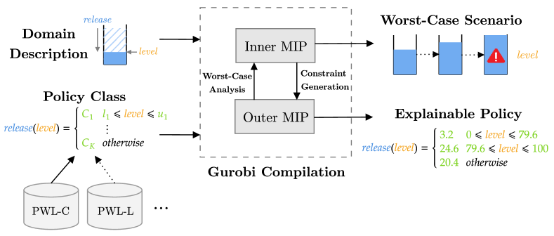
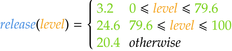
Figure 1: Reservoir control is used as an illustrative example. Left: an overview of CGPO, which consists of a domain description and policy representation compiled to a bilevel mixed-integer program (MIP), in which the inner problem computes the worst-case trajectories for the current policy while the outer problem updates the policy via constraint-generation. The result is a worst-case scenario, a concrete policy within the expressivity class, and a gap on its performance. Right: three optimal (i.e. zero-gap) policies produced upon termination across several piecewise policy classes. Crucially, our framework provides the ability to derive highly compact (e.g. memory and time-efficient to execute), intuitive and nonlinear policies, with strong bound guarantees on policy performance.

In this paper, we aim to provide a solution approach to optimize and provide strong performance bound guarantees on structured and compact DC-MDP policies under various expressivity classes of policy, reward, and (nonlinear) transition dynamics. Our specific contributions are as follows:

1. We propose a novel nonlinear bi-level optimization framework called Constraint-Generation Policy Optimization (CGPO), that admits a clever reduction to an iterative constraint-generation algorithm that can be readily implemented using standard MIP solvers (cf. Figure 1). State-of-the-art nonlinear solvers often leverage spacial branch-and-bound techniques, which can provide not only optimal solutions for large mixed integer linear programs (MILP), but also bounded optimality guarantees for many cases of mixed integer nonlinear programs (MINLP) (Castro 2015). We efficiently handle stochastic DC-MDPs using marginalization, or chance-constraints (Farina, Giulioni, and Scattolini 2016) to provide probabilistic guarantees on policy performance.

2. If the constraint generation algorithm terminates, we provide a guarantee that we have found the optimal policy within the given policy expressivity class (Theorem 1). Further, even when constraint generation does not terminate, our algorithm provides a tight optimality bound on the performance of the computed policy at each iteration and the scenario where the policy performs worst (and as a corollary, for any externally provided policy).

3. We provide a road map to characterize the optimization problems in (1) above – and their associated expressivity classes – for different expressivity classes of policies and state dynamics, ranging from MILP, to polynomial programming, to nonlinear programs (cf. Table 1). This information is beneficial for reasoning about which optimization techniques are most effective for different combinations of DC-MDP and policy class expressivity.

4. Finally, we provide a variety of experiments demonstrating the range of rich applications of CGPO under linear and nonlinear dynamics and various policy classes. Critically, we derive bounded optimal solutions for a range of problems, including linear inventory management, reservoir control, and a highly nonlinear VTOL control problem. Further, since our policy classes are compact by design, we can also directly inspect and analyze these policies (cf. Figure 2). To facilitate policy interpretation and diagnostics, we can compute the state and exogenous noise trajectory scenario that attains the worst-case error bounds for a policy (cf. Figure 5) as well as a counterfactual explanation of what action should have been taken in comparison to what the policy prescribes.

Preliminaries

Function Classes

We first define some important classes of functions commonly referred to throughout the paper. Let $\mathcal{X}$ and $\mathcal{Y}$ be arbitrary sets. A function $f:\mathcal{X}\to\mathcal{Y}$ is called piecewise (PW) if there exist functions $f_{1},\dots f_{K},f_{K+1}:\mathcal{X}\to\mathcal{Y}$ and disjoint Boolean predicates $\mathcal{P}_{1}\dots\mathcal{P}_{K}:\mathcal{X}\to\{0,1\}$, such that for any $x\in\mathcal{X}$, $\forall i,j\!\neq\!i\,\,\mathcal{P}_{i}(x)\!=\!1\,\Rightarrow\,\mathcal{P}_{j}(x)\!=\!0$ and

$$f(x)=\begin{cases}f_{1}(x),&\mbox{ if }\mathcal{P}_{1}(x)=1,\\ &\vdots\\ f_{K}(x)&\mbox{ if }\mathcal{P}_{K}(x)=1,\\ f_{K+1}(x)&\mbox{ otherwise}.\end{cases}$$ (1)

Both predicates $\mathcal{P}_{i}$ and cases ${f}_{i}$ can be either linear or nonlinear. In this paper, we consider the following classes:

• constant (C), i.e. $f_{i}(\mathbf{x})=C$

• discrete (D), same as restricted values of C

• simple (axis-aligned) linear functions (S), i.e. $f_{i}(\mathbf{x})=b_{i}+w_{i}\times x_{j}$, where $j\in\{1,2\dots n\}$ and $b_{i},w_{i}\in\mathbb{R}$

• linear (L), i.e. $f_{i}(\mathbf{x})=b_{i}+\mathbf{w}_{i}^{T}\mathbf{x}$

• bilinear (B), i.e. $f_{i}(\mathbf{x})=x_{1}\times x_{2}+x_{2}\times x_{3}$

• quadratic (Q), i.e. $f_{i}(\mathbf{x})=b_{i}+\mathbf{w}_{i}^{T}\mathbf{x}+\mathbf{x}^{T}M_{i}\mathbf{x}$, where $M_{i}\in\mathbb{R}^{n\times n}$

• polynomial (P) of order $m$, i.e. $f_{i}(\mathbf{x})=\sum_{j_{1}=1}^{m}\dots\sum_{j_{n}=1}^{m}w_{i,j_{1},\dots j_{n}}\prod_{k=1}^{n}x_{k}^{j_{k}}$

• general nonlinear (N), i.e. $f(\mathbf{x})=e^{b_{i}+\mathbf{w}_{i}^{T}\mathbf{x}}$.

In a similar way, we can also consider analogous functions over integer (I) domains $\mathcal{X}$ or $\mathcal{Y}$, or mixed discrete-continuous (M) domains. $\mathcal{P}_{i}$ can be characterized in a similar way based on whether the constraint, or set of constraints, defining it are constant, linear, bilinear, quadratic, etc.

We also introduce a convenient notation to describe general PW functions by concatenating the expressivity classes of their constraints $\mathcal{P}_{i}$ and case functions $f_{i}$. For example, PWS-C describes a piecewise function on $\mathbb{R}^{n}$ with univariate axis-aligned constraints and constant values, while PWS-L describes a similar function but with linear values, i.e.:

$$f(\mathbf{x})=\begin{cases}b_{1}+\mathbf{w}_{1}^{T}\mathbf{x},&\mbox{ if }l_{1}\leq c_{1}+v_{1}x_{i_{1}}\leq u_{1},\\ &\vdots\\ b_{K}+\mathbf{w}_{K}^{T}\mathbf{x}&\mbox{ if }l_{K}\leq c_{K}+v_{K}x_{i_{K}}\leq u_{K},\\ b_{K+1}+\mathbf{w}_{K+1}^{T}\mathbf{x}&\mbox{ otherwise}.\end{cases}$$

We also append the number of cases $K$ to the notation, i.e. PWS1-L describes a piecewise linear function as above with $K=1$, and we assume that $K$ is finite in our derivation. More generally, for functions in PWL, PWP and PWN, constraints could also be conjunctions of other simpler constraints, i.e. $\mathcal{P}_{i}(\mathbf{x})=\bigwedge\limits_{j=1}^{c}\left\{l_{ij}\leq b_{ij}+\mathbf{w}_{ij}^{T}\mathbf{x}\leq u_{ij}\right\}$.

Mathematical Programming

Given a function $f:\mathcal{X}\to\mathcal{Y}$ and Boolean predicate $\mathcal{P}:\mathcal{X}\to\{0,1\}$, we define the general mathematical program:

$$\min_{x\in\mathcal{X}} f(x)\quad\textrm{s.t.}\quad \mathcal{P}(x)=1.$$

Important standard expressivity classes of mixed-integer program (MIP) optimization problems, i.e. those with discrete and continuous decision variables, include:

• mixed-integer linear (MILP), i.e. $f$, $\mathcal{P}$ are both L

• mixed-integer bilinearly constrained (MIBCP), i.e. $f$ is L and $\mathcal{P}$ is B

• mixed-integer quadratic (MIQP), i.e. $f$ is Q and $\mathcal{P}$ is L

• quadratically constrained quadratic (QCQP), i.e. $f$, $\mathcal{P}$ are both Q

• polynomial (PP), i.e. $f$, $\mathcal{P}$ are both P

• mixed-integer nonlinear (MINLP), i.e. $f$, $\mathcal{P}$ are both N.

Branch-and-bound (Morrison et al. 2016) is a powerful search technique for finding optimal solutions to mathematical programs, and is a key component of modern state-of-the-art nonlinear optimization software. One advantage of this class of algorithms is the ability to maintain upper and lower bounds on the minimal objective value of any linear or nonlinear MIP (and thus the optimal solution in any branch of the search tree), whose difference is called the optimality gap; when this gap is zero, an optimal solution has been found. Moreover, some packages such as Gurobi (Gurobi Optimization, LLC 2023), which we use to perform the necessary compilations in CGPO in our experiments, also support a variety of nonlinear mathematical operations via piecewise-linear approximation (Castro 2015).

Discrete-Continuous Markov Decision Processes

A Discrete-Continuous Markov decision process (DC-MDP) is a tuple $\langle\mathcal{S},\mathcal{A},P,r\rangle$, where $\mathcal{S}$ is a set of states, $\mathcal{A}$ is a set of actions or controls. $\mathcal{S}$ and $\mathcal{A}$ may be discrete, continuous, or mixed. $P(\mathbf{s},\mathbf{a},\mathbf{s}^{\prime})$ is the probability of transitioning to state $\mathbf{s}^{\prime}$ immediately upon choosing action $\mathbf{a}$ in state $\mathbf{s}$, and $r(\mathbf{s},\mathbf{a},\mathbf{s}^{\prime})$ is the corresponding reward received. We assume that $r$ is uniformly bounded, i.e. there is a $B<\infty$ such that $r(\mathbf{s},\mathbf{a},\mathbf{s}^{\prime})\leq B$ holds for all $\mathbf{s},\mathbf{a},\mathbf{s}^{\prime}$.

Given a planning horizon of length $T$ (assumed fixed in our setting), the value of a (open-loop) plan $\alpha=[\mathbf{a}_{1},\dots\mathbf{a}_{T}]\in\mathcal{A}^{T}$ starting in state $\mathbf{s}_{1}$ is

$$V(\alpha,\mathbf{s}_{1})=\mathbb{E}_{\mathbf{s}_{t+1}\sim P(\mathbf{s}_{t},\mathbf{a}_{t},\cdot)}\!\left[\sum_{t=1}^{T}r(\mathbf{s}_{t},\mathbf{a}_{t},\mathbf{s}_{t+1})\right].$$

A policy $\pi=[\pi_{1},\dots\pi_{T}]$ is a sequence of mappings $\pi_{t}:\mathcal{S}\to\mathcal{A}$, whose value is defined as

$$V(\pi,\mathbf{s}_{1})=\mathbb{E}_{\mathbf{s}_{t+1}\sim P(\mathbf{s}_{t},\pi_{t}(\mathbf{s}_{t}),\cdot)}\!\left[\sum_{t=1}^{T}r(\mathbf{s}_{t},\pi_{t}(\mathbf{s}_{t}),\mathbf{s}_{t+1})\right].$$

Dynamic programming approaches such as value or policy iteration can compute an optimal horizon-dependent policy $\pi_{H}^{*}$ (Puterman 2014), but do not directly apply to DC-MDPs with infinite or continuous state or action spaces.

Our goal is to compute an optimal stationary reactive policy $\pi^{*}$ (Bueno et al. 2019) that minimizes the error in value (i.e. regret) relative to $\pi_{H}^{*}$ over all initial states of interest $\mathcal{S}_{1}\subseteq\mathcal{S}$, and all stationary policies $\Pi$, i.e.

$$\pi^{*}\in\operatorname*{arg\,min}_{\pi\in\Pi}\max_{\mathbf{s}_{1}\in\mathcal{S}_{1}}\left[V(\pi_{H}^{*},\mathbf{s}_{1})-V(\pi,\mathbf{s}_{1})\right].$$ (2)

In practical applications, the policy class is typically restricted to some class of function approximations $\tilde{\Pi}\subset\Pi$. A variety of planning approaches can compute the optimal policies $\tilde{\pi}^{*}\in\tilde{\Pi}$ for this problem, including straight-line planning that scales well in practice but does not learn policies (Wu, Say, and Sanner 2017; Raghavan et al. 2017), and deep reactive policy (Bueno et al. 2019; Low, Kumar, and Sanner 2022), MCTS (Świechowski et al. 2023) and similar approaches that learn neural network policies but cannot provide concrete bounds on performance, nor compactness or ease of interpretation of the inferred policy map.

Methodology

Our main contribution is a novel iterative constraint generation algorithm for policy optimization with structured (i.e. piecewise) policies. We begin with a simple worked example to illustrate the intuition behind our approach. Next, we present the constraint generation approach for general deterministic DC-MDPs, and then describe the chance-constraints modification that works with high probability for stochastic DC-MDPs.

Worked Example

In order to shed some intuition on our constraint-generation approach in the general MDP setting, we illustrate our approach in the context of a one-dimensional “navigation” type problem.

Domain Description

Let the state $s_{t}$ denote the continuous position of a particle on $\mathbb{R}$ at epoch $t=1,2$, and let the action be a continuous unbounded displacement $a_{t}$ applied to the particle, so that the state updates according to $s_{t+1}=s_{t}+a_{t}$. Thus, $\mathcal{S}=\mathcal{A}=\mathbb{R}$ and suppose further that $\mathcal{S}_{1}=[0,5]$. If the target position is designated as $10$, we formulate the reward as $r(s_{t+1})=-|s_{t+1}-10|$, and thus the value function is $V(a_{1},s_{1})=-|s_{1}+a_{1}-10|$.

The Outer Problem

For ease of illustration, we focus our attention on linear policies of the form $a_{t}=b+ws_{t}$, where $(w,b)$ are real-valued decision variables to be optimized. The goal is to find the optimal policy parameters:

$$\min_{(w,b)\in\mathbb{R}^{2}}\max_{s_{1}\in[0,5]}\max_{a_{1}\in\mathbb{R}}\,[V(a_{1},s_{1})-V((w,b),s_{1})],$$

where $V((w,b),s_{1})=-|s_{1}+b+ws_{1}-10|$ is the value of the linear policy. However, this problem is not directly solvable due to the inner $\max$, but it can be written as

$$\min_{(w,b)\in\mathbb{R}^{2},\,\varepsilon\in[0,\infty)}\varepsilon,\quad\textrm{s.t.}\quad\varepsilon\geq V(a_{1},s_{1})-V((w,b),s_{1}),$$

where constraints are enumerated by all possible $(s_{1},a_{1})$ pairs. Since the number of constraints is infinite for continuous states or actions, it suggests a constraint generation approach, where a large set of diverse $(s_{1},a_{1})$ pairs are used to “build up” the constraint set one at a time, decoupling the overall problem into a sequence of solvable MIPs. However, a key question arises: which state-action pairs $(s_{1},a_{1})$ should be considered for inclusion into the outer problem? While a number of different reasonable choices (diversity, coverage) exist, a logical choice is to select the state action pairs in relation to which the policy $\pi_{\mathbf{w}}$ performs worst.

Solving the Outer Problem

The outer problem thus maintains a finite subset of constraints from the infinitely-constrained problem. We begin with an arbitrary $(s,a)$-pair, which forms the first constraint of the outer problem. For illustration, we select $(s_{1},a_{1})=(0,0)$, which defines the first constraint of the outer problem $\varepsilon\geq V(0,0)-V((w,b),0)=-10+|b-10|$. The outer problem becomes:

$$\min_{w,b\in\mathbb{R},\,\varepsilon\in[0,\infty)}\,\varepsilon,\quad\mathrm{s.t.}\quad\varepsilon\geq-10+|b-10|.$$

Recognizing that the minimum of the r.h.s. of the constraint is attained at $b^{*}=10$, and $w^{*}$ arbitrary, we select $(w^{*},b^{*})=(0,10)$ as the solution of the outer problem with optimal $\varepsilon=0$. Next, we will try to improve upon the policy by adding an additional constraint to the outer problem.

Solving the Inner Sub-Problem

To accomplish this, we need to add a new scenario $(s_{1},a_{1})$ in relation to which the policy $(w,b)=(0,10)$ performs worst. Thus, we solve:

$$\max_{s_{1}\in[0,5],a_{1}\in\mathbb{R}}[V(a_{1},s_{1})-V((w,b),s_{1})]$$

$$=\max_{s_{1}\in[0,5],a_{1}\in\mathbb{R}}[-|s_{1}+a_{1}-10|+s_{1}],$$

from which we find $(s_{1}^{*},a_{1}^{*})=(5,5)$. The optimal value of this problem is positive, so it represents a potentially binding constraint in the outer problem. Thus, we could improve upon the policy by adding the corresponding constraint.

Solving the Outer Problem Again

We add the constraint corresponding to this scenario to the outer problem:

$$\min_{(w,b)\in\mathbb{R}^{2},\,\varepsilon\in[0,\infty)}\quad\varepsilon\qquad\textrm{s.t.}\quad\varepsilon \geq-10+|b-10|$$

$$\varepsilon \geq|b+5w-5|,$$

whose new solution can be found as $b^{*}=10,w^{*}=-1$ with optimal $\varepsilon=0$. Finally, the worst-case scenario for this new policy can be found from the inner sub-problem, whose optimal solution (among many) is $(s_{1}^{*},a_{1}^{*})=(0,10)$ with value zero. Therefore, this worst-case corresponds to a non-binding constraint in the outer problem, and we terminate with the optimal linear policy $\pi^{*}(s_{1})=10-s_{1}$. $\square$

Constraint Generation for Deterministic DC-MDPs

We now extend the intuition above to the general deterministic MDP setting. We assume that $\pi$ can be compactly identified by a vector $\mathbf{w}\in\mathcal{W}$ of decision variables, and we shall write $V(\mathbf{w},\mathbf{s}_{1})$ to denote the value $V(\pi_{\mathbf{w}},\mathbf{s}_{1})$ of the policy $\pi_{\mathbf{w}}$ parameterized by $\mathbf{w}$. In what follows, we focus our attention on approximate policy sets $\tilde{\Pi}_{\mathcal{W}}=\{\pi_{\mathbf{w}}:\mathbf{w}\in\mathcal{W}\}$ that can be compactly described by piecewise functions (1).

First, observe that for every possible initial state $\mathbf{s}_{1}$, there exists a fixed optimal plan $\alpha^{*}=[\mathbf{a}_{1}^{*},\dots\mathbf{a}_{T}^{*}]$ such that $V(\alpha^{*},\mathbf{s}_{1})=V(\pi_{H}^{*},\mathbf{s}_{1})$. On the other hand, since we only have access to an expressivity class of approximate policies $\tilde{\Pi}_{\mathcal{W}}$, the error $\varepsilon(\mathbf{w},\mathbf{s}_{1})$ of $\pi_{\mathbf{w}}$ in state $\mathbf{s}_{1}$ relative to $V(\pi_{H}^{*},\mathbf{s}_{1})$ (according to (2)) must be

$$\varepsilon(\mathbf{w},\mathbf{s}_{1})\geq\max_{\alpha\in\mathcal{A}^{T}}V(\alpha,\mathbf{s}_{1})-V(\mathbf{w},\mathbf{s}_{1}),$$ (3)

and thus the worst-case error $\varepsilon(\mathbf{w})$ of $\mathbf{w}$ is

$$\varepsilon(\mathbf{w})\geq\max_{\mathbf{s}_{1}\in\mathcal{S}_{1}}\max_{\alpha\in\mathcal{A}^{T}}\left[V(\alpha,\mathbf{s}_{1})-V(\mathbf{w},\mathbf{s}_{1})\right].$$ (4)

However, since we seek the approximate optimal policy $\tilde{\pi}^{*}\in\tilde{\Pi}_{\mathcal{W}}$, we can directly minimize (4) over $\mathcal{W}$, obtaining the following infinitely-constrained mixed-integer program:

$$\min_{\mathbf{w}\in\mathcal{W},\,\varepsilon\in[0,\infty)} \varepsilon$$ (5)

s.t. $$\varepsilon\geq\max_{\mathbf{s}_{1}\in\mathcal{S}_{1}}\max_{\alpha\in\mathcal{A}^{T}}\big{[}V(\alpha,\mathbf{s}_{1})-V(\mathbf{w},\mathbf{s}_{1})\big{]}.$$

However, the constraint is highly nonlinear, turning (5) into a bi-level program and making analysis of this particular formulation difficult. Instead, since the $\max$’s must hold for all states and actions, we can rewrite the problem (5) as:

$$\min_{\mathbf{w}\in\mathcal{W},\,\varepsilon\in[0,\infty)} \varepsilon$$ (6)

s.t. $$\varepsilon\geq V(\alpha,\mathbf{s}_{1})-V(\pi,\mathbf{s}_{1})$$

$$\quad\,\forall\alpha\in\mathcal{A}^{T},\,\mathbf{s}_{1}\in\mathcal{S}_{1}.$$

The goal is therefore to solve (6), which is still infinitely-constrained when $\mathcal{S}$ or $\mathcal{A}$ are infinite spaces. Instead, we solve it by splitting the $\min$ over $\mathcal{W}$ and the $\max$ over $(\alpha,\mathbf{s}_{1})$ into two problems, and apply constraint generation (Blankenship and Falk 1976; Chembu et al. 2023). Specifically, starting with a fixed arbitrary scenario $(\mathbf{s}_{1},\alpha)$, we form the constraint set $\mathcal{C}=\{(\mathbf{s}_{1},\alpha)\}$, and then repeatedly solve the following two problems:

• Outer Problem: Solve (6) over the finite constraint set $\mathcal{C}$ to obtain policy $\mathbf{w}_{1}^{*}\in\mathcal{W}$.

• Inner Problem: Solve (4):

  $$(\mathbf{s}_{1}^{*},\alpha^{*})\in{\arg\!\max}_{\mathbf{s}_{1}\in\mathcal{S}_{1},\alpha\in\mathcal{A}^{T}}\left[V(\alpha,\mathbf{s}_{1})-V(\mathbf{w}_{0}^{*},\mathbf{s}_{1})\right],$$

  for the highest-error scenario for $\mathbf{w}_{1}^{*}$, and append it to $\mathcal{C}$.

These two steps are repeated until the constraint added to the outer problem is no longer binding, i.e. $V(\alpha^{*},\mathbf{s}_{1}^{*})-V(\mathbf{w}_{t}^{*},\mathbf{s}_{1}^{*})\leq 0$, since the solution of the outer problem will not change with the addition of the constraint. We name this approach Constraint-Generation Policy Optimization (CGPO) (see Figure 1). Intuitively, we can view CGPO as a policy iteration algorithm where the inner problem adversarially critiques the policy with a worst-case trajectory and the outer problem improves the policy w.r.t. all critiques.

Remarks

Upon termination, GCPO’s use of constraint generation guarantees an optimal (i.e., lowest error) policy within the specified policy class (see Theorem 1). Further, while we cannot provide a general finite-time guarantee of termination with an optimal policy, CGPO is an anytime algorithm that provides a best policy and a bound on performance at each iteration. Remarkably, CGPO is applicable for solving infinite state/action bi-level policy optimization problems by exploiting the fact that only several constraints may be active at the optimal solution. In addition, at each stage, the solution to the inner problem allows us to interpret and analyze the state with the worst-case policy performance with respect to $\pi$ (cf. Figure 5), and generate a counterfactual explanation of what actions should have been made.

Chance Constraints for Stochastic MDPs

We now turn our attention to MDPs with stochastic transitions, which are considerably more difficult to handle since they cannot be reformulated directly in the form (5).

A number of approaches could be used to encode stochastic variables, including sample approximation (SAA) (Kleywegt, Shapiro, and Homem-de Mello 2002) and hindsight encoding (Raghavan et al. 2017) on the inner constraints, which would typically lead to a blowup in the problem size. Chance-constrained approaches (Ono et al. 2015; Farina, Giulioni, and Scattolini 2016; Ariu et al. 2017) instead generate constraints that hold with high probability, which often alleviate the computational burden at the expense of introducing some degree of (controllable) bias. Motivated by the recent applications of chance-constraints in planning and control, we take the latter approach, which will lead to a particularly elegant bi-level reformulation of (6) as we now see.

To achieve this, we will require that the state transition function $P(\mathbf{s},\mathbf{a},\mathbf{s}^{\prime})$ has a natural reparameterization as a deterministic function of $(\mathbf{s}$, $\mathbf{a})$ of some exogenous i.i.d. noise variable $\xi$ with density $q(\cdot)$ on support $\Xi$, e.g. $\mathbf{s}^{\prime}=g(\mathbf{s},\mathbf{a},\xi)$ (Bueno et al. 2019). Given a “confidence” threshold $p\in(0,1)$ close to 1, we also assume the existence of a computable interval $\Xi_{p}=[\xi_{l},\xi_{u}]$ such that $\mathbb{P}\!\left(\xi_{l}\leq\xi\leq\xi_{u}\right)\geq p$.

Thus, we can repeat the reasoning of the previous section, by considering the worst case not only over $\mathbf{s}_{1}$, but also over possible trajectories or rollouts $\xi_{1:T}=[\xi_{1},\dots\xi_{T}]\in\Xi_{p}^{T}$. The analogue of (5) in the stochastic setting is:

$$\min_{\mathbf{w}\in\mathcal{W},\,\varepsilon\in[0,\infty)} \varepsilon$$ (7)

s.t. $$\varepsilon\geq\max_{\mathbf{s}_{1}\in\mathcal{S}_{1}}\max_{\xi_{1:T}\in\Xi_{p}^{T}}\max_{\alpha\in\mathcal{A}^{T}}\big{[}$$

$$\quad V(\alpha,\mathbf{s}_{1},\xi_{1:T})-V(\mathbf{w},\mathbf{s}_{1},\xi_{1:T})\big{]},$$

where $V(\cdot,\mathbf{s}_{1},\xi_{1:T})$ corresponds to the total reward of the policy or plan accumulated over trajectory $\xi_{1:T}$ starting in $\mathbf{s}_{1}$. In the stochastic setting, it is important to note that $\varepsilon$ only holds with probability $p^{T}$ for a horizon $T$ problem. In practice, we choose $p$ such that $p^{T}=\alpha$ equates to some desired global probability bound on the entire planning trajectory $\alpha$.

Once again, (7) can be reformulated as:

$$\min_{\mathbf{w}\in\mathcal{W},\,\varepsilon\in[0,\infty)} \varepsilon$$ (8)

s.t. $$\varepsilon\geq V(\alpha,\mathbf{s}_{1},\xi_{1:T})-V(\mathbf{w},\mathbf{s}_{1},\xi_{1:T}),$$

$$\quad\,\forall\alpha\in\mathcal{A}^{T},\,\mathbf{s}_{1}\in\mathcal{S}_{1},\,\xi_{1:T}\in\Xi_{p}^{T}.$$

Therefore, we can again apply constraint generation to solve this problem in two stages, in which the inner optimization produces not only a worst-case initial state and action sequence, but also the disturbances $\xi_{1:T}^{*}$ that reproduce all future worst-case state realizations $\mathbf{s}_{2},\dots\mathbf{s}_{T}$. A complete description of this algorithm is provided in Algorithm 1.

Algorithm 1 Constraint-Generation Policy Optimization (CGPO)

  Initialize $p\in(0,1)$ and compute $\Xi_{p}$

  Initialize $\mathbf{s}_{1}\in\mathcal{S}_{1}$, $\xi_{1:T}\in\Xi_{p}^{T}$ and $\alpha\in\mathcal{A}^{T}$ arbitrarily

  Initialize constraint set $\mathcal{C}_{0}=\{(\mathbf{s}_{1},\xi_{1:T},\alpha)\}$

  Set $t=0$

  Step 1: Solve the outer problem:

$$(\mathbf{w}_{t}^{*},\varepsilon_{t}^{*})\in {\arg\!\min}_{\mathbf{w}\in\mathcal{W},\,\varepsilon\in[0,\infty)}\,\varepsilon$$

$$\mathrm{s.t.} \varepsilon\geq V(\alpha,\mathbf{s}_{1},\xi_{1:T})-V(\mathbf{w},\mathbf{s}_{1}),$$

$$\forall\,(\mathbf{s}_{1},\xi_{1:T},\alpha)\in\mathcal{C}_{t}$$

  Step 1: Solve the inner problem:

$$(\mathbf{s}_{1}^{*},\xi_{1:T}^{*},\alpha^{*})\in{\arg\!\max}_{\mathbf{s}_{1}\in\mathcal{S}_{1},\,\xi_{1:T}\in\Xi_{p}^{T},\,\alpha\in\mathcal{A}^{T}}\big{[}$$

$$\qquad V(\alpha,\mathbf{s}_{1},\xi_{1:T})-V(\mathbf{w}_{t}^{*},\mathbf{s}_{1},\xi_{1:T})\big{]}$$

Step 3: Check convergence:

  if $V(\alpha^{*},\mathbf{s}_{1}^{*},\xi_{1:T}^{*})-V(\mathbf{w}_{t}^{*},\mathbf{s}_{1}^{*},\xi_{1:T}^{*})\leq 0$ then

     Terminate with policy $\mathbf{w}_{t}^{*}$ and error $\varepsilon_{t}^{*}$

  else

     Set $\mathcal{C}_{t+1}=\mathcal{C}_{t}\cup\{(\mathbf{s}_{1}^{*},\xi_{1:T}^{*},\alpha^{*})\}$

     Set $t=t+1$ and go to Step 1

  end if

Remarks

In discrete-state problems, we can instead analytically marginalize out the exogenous noise to produce an “expected” transition model $\mathbf{s}^{\prime}=\sum_{\xi\in\Xi}g(\mathbf{s},\mathbf{a},\xi)q({\xi})$. For distributions on an infinite support, i.e. $\mathbb{Z}$ or $\mathbb{N}$, it is possible to marginalize over a truncated noise distribution $\tilde{q}({\xi})\propto q(\xi)1\{\xi\leq\xi_{p}\}$, where $p\in(0,1)$ is a parameter close to 1, and $\xi_{p}$ is chosen such that $\mathbb{P}\!\left(\xi\leq\xi_{p}\right)\geq p$.

Discussion of Convergence

Finite-time termination of Algorithm 1 is impossible to show without strong assumptions (i.e. convexity). However, we can still show under mild assumptions that, if Algorithm 1 terminates at some iteration $t$, then $\mathbf{w}_{t}^{*}$ is optimal in $\mathcal{W}$ (with probability $p^{T}$ in the stochastic case).

Theorem 1.

If $\mathcal{S}_{1}$, $\mathcal{A}$, $\Xi_{p}$ and $\mathcal{W}$ are non-empty compact subsets of Euclidean space, $V(\alpha,\mathbf{s},\xi_{1:T})$ and $V(\mathbf{w},\mathbf{s},\xi_{1:T})$ are continuous, and Algorithm 1 terminates at iteration $t$, then $\mathbf{w}_{t}^{*}$ is optimal for problem (8).

Proof.

The proof is adapted from Theorem 2.1 in Blankenship and Falk (1976), as discussed in the Appendix. ∎

Remarks

Termination of CGPO guarantees that $\mathbf{w}_{t}$ is optimal in $\tilde{\Pi}_{\mathcal{W}}$, and $\varepsilon_{t}^{*}$ is the corresponding optimality gap. Moreover, if $\varepsilon_{t}^{*}=0$ and the MDP is deterministic, then $\pi_{\mathbf{w}^{*}}$ is the optimal policy for the MDP. This means we can use the gap estimate as a principled way to compare and validate different policy classes in practice. Blankenship and Falk (1976) also provides a modified approach (Algorithm 2.2) identical to CGPO, except for the removal of constraints that become non-binding from the outer problem at each iteration. If the problem $\max_{\mathbf{w}\in\mathcal{W}}V(\mathbf{w},\mathbf{s}_{1})$ is convex, convergence of CGPO could be established.

Analysis of Problem Expressivity Classes

In Table 1, we discuss the relationship between the expressivity classes of policies and state transition dynamics and the resulting classes of the inner and outer optimization problems. The policy classes of interest include PWS-C, PWL-C, PWS-L, PWL-L, PWN-N and the different variants of piecewise polynomial policies. Meanwhile, expressivity classes for state dynamics and reward include linear, polynomial and general nonlinear functions (their piecewise counterparts generally fall under the same expressivity classes, and are excluded for brevity).

Interestingly, when the policy and state dynamics are both linear, the outer problem is a PP. To see this, consider the transition function $s^{\prime}=s+a$, and the policy $a=ws$. Then:

$$s^{\prime} =s+a=s+ws=(w+1)s$$

$$a^{\prime} =ws^{\prime}=w(w+1)s=O(w^{2})$$

$$s^{\prime\prime} =s^{\prime}+a^{\prime}=(w+1)s+w(w+1)s=(w+1)^{2}s$$

$$a^{\prime\prime} =ws^{\prime\prime}=w(w+1)^{2}s=O(w^{3}),$$

which are polynomial in $w$. In a similar vein, a PWL-C policy and linear dynamics result in a MIBCP outer problem due to the bilinear interaction between successor state decision variables and policy weights in the linear conditions.

Our experiments in the next section empirically evaluate PWS-C and PWS-L policies with linear dynamics, and Q policies with nonlinear dynamics. This requires solving mixed-integer problems with large numbers of decision variables ranging from MILP to PP to MINLP. However, as algorithmic improvements in nonlinear optimizers continue to improve their search efficiency, we expect the performance of CGPO will also improve accordingly, allowing solutions for larger problems and policy expressivity classes.

Policy	L	P	N
PWS-{C, D}	MILP	PP	MINLP
PWL-{C, D}	MILP/MIBCP	PP	MINLP
S, L	MILP/PP	PP	MINLP
PW{S,L}-{S,L}	MILP/PP	PP	MINLP
PW{S,L,P}-P	PP	PP	MINLP
Q	PP	PP	MINLP
PWN-N	MINLP	MINLP	MINLP

Table 1: Problem classes of the inner/outer optimization problems in Algorithm 1 for different expressivity classes of dynamics/reward (columns) and policies (rows).

$reorder=4-stock$ $reorder=\begin{cases}5-stock&\mbox{ if }-1\leq stock\leq 2\\ 3-stock&\mbox{ otherwise }\end{cases}$

$release_{1}=\begin{cases}33.23&\mbox{ if }65.06\leq level_{1}\leq 100\\ 1.08&\mbox{ otherwise }\end{cases}$ $release_{2}=\begin{cases}72.91&\mbox{ if }100\leq level_{2}\leq 200\\ 0.2&\mbox{ otherwise }\end{cases}$

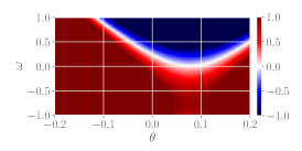
$F=0.6-15.4\theta-2.3\omega+100\theta^{2}-1.5\omega^{2}$

Figure 2: Optimal S/PWS-S policy for inventory (left), PWS-C policy for reservoir (middle), Q policy for VTOL (right).

Implementation Details

Relational Dynamic influence Diagram Language (RDDL) is a structured planning domain description language particularly well-suited for modelling problems with stochastic effects (Sanner 2010). Our domains are therefore coded in RDDL (please see supplementary material for the domain descriptions) and we wrote a general-purpose routine for compiling RDDL code into a Gurobi mixed integer program formulation using the pyRDDLGym interface (Taitler et al. 2022). In order to compute the tightest possible bounds on decision variables in the MIP compilation, we use interval arithmetic (Hickey, Ju, and Van Emden 2001).

Empirical Evaluation

We now empirically validate the soundness and performance of Algorithm 1 on several standard MDPs. The goal of the empirical evaluation is to answer the following research questions:

1. Does CGPO recover exact solutions when the ideal policy class is known? How does it perform if the optimal policy class is not known?

2. How do different policy expressivity classes perform per constraint generation iteration for each problem?

3. How can we explain the results from the worst-case analysis to gain further insight about a policy?

To answer these questions, we evaluate on linear inventory control, linear reservoir management, and nonlinear VTOL control domains. Full descriptions are provided in the Appendix, including analysis of an additional nonlinear Boolean-action “intercept” domain. Inventory control has provably optimal PWS-S policies, whereas no optimal policy class is known explicitly for reservoir control; this allows us to answer Q1. The incorporation of the nonlinear VTOL problem will allow us to evaluate how CGPO scales across a variety of expressivity classes for linear/nonlinear dynamics. A public github repository allows reproduction of all results and application of CGPO to arbitrary RDDL domains.

Domain Descriptions

Linear Inventory

State $s_{t}$ describes the discrete level of stock available for a single good, action $a_{t}$ is the discrete reorder quantity, demand $\xi_{t}$ is stochastic and distributed as discrete uniform. Backlogging of inventories is allowed and is represented by negative $s_{t}$. The reward function consists of unit costs for product purchasing, excess and shortage of inventory. A planning horizon of $T=8$ is used. For this domain and reservoir below, we focus on learning factorized piecewise policies, i.e. C, S, PWS-C and PWS-S.

Linear Reservoir

The objective is to manage the water levels in a system of interconnected water reservoirs. State $s_{t,r}$ represents the continuous water level of reservoir $r$ with capacity $M_{r}$, action $a_{t,r}$ is the continuous amount of water released, and rainfall $\xi_{t,r}$ is a clipped normally-distributed random variable (to allow possibility of no rainfall). Each reservoir $r$ is connected to a set $U(r)$ of upstream reservoirs. Reward linearly penalizes any excess water level above $H_{r}$ and below $L_{r}$. We use $T=10$.

Nonlinear VTOL Control

Lastly, we consider a highly nonlinear aircraft VTOL control problem illustrated in Fig. 3. The objective is to balance two masses on opposing ends of a long pole, by applying a force to one of the two masses. The state consists of the angle $\theta_{t}$ and angular velocity $\omega_{t}$ of the pole, and the action is the force $F_{t}\in[0,1]$ applied to the mass. Time is discretized into intervals of length $\tau=0.1$ seconds, and we set $T=6$. The reward penalizes the difference between the pole angle and a target angle, as well as the magnitude of the force to ensure smoothness. We optimize for nonlinear quadratic policies.

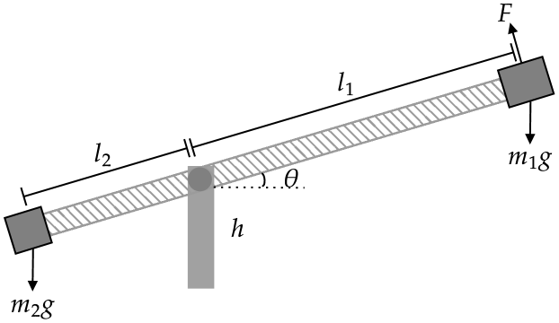
Figure 3: The nonlinear VTOL control problem.

Nonlinear Intercept

To demonstrate an example of Discrete (Boolean) action policy optimization over nonlinear continuous state dynamics with independently moving but interacting projectiles, we turn to an intercept problem inspired by Scala et al. (2016). Space restrictions require us to relegate details and results to the Appendix, but we remark here that CGPO is able to derive an optimal policy.

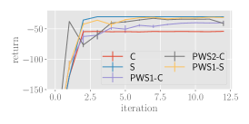
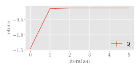
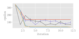
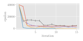
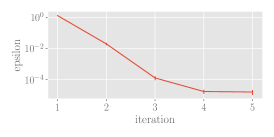
Figure 4: Simulated return (top row) and worst-case error $\varepsilon^{*}$ (bottom row) on inventory (left column), reservoir (centre column) and VTOL (right column) over 100 independent roll-outs as a function of the number of iterations of constraint generation. Bars represent 95% confidence intervals calculated using 10 independent runs of Algorithm 1.

Empirical Results

MIPs are solved to an optimality gap of 5% and we use $p=0.995$. Fig. 2 illustrates examples of policies learned in a typical run of Algorithm 1. Fig. 4 compares the empirical (simulated) returns and error bounds $\varepsilon^{*}$ (optimal objective value of the inner problem) across different policy classes.

As hypothesized, CGPO can recover exact $(s,S)$ control policies for inventory control in the PWS-S class, which together with S policies achieve the lowest error and best return across all policy classes. Interestingly, as Fig. 4 shows, C and PWS-C policies perform relatively poorly even for $K=2$, but as expected, the error decreases with the policy expressivity class and the number of cases. This is intuitive, as Fig. 2 shows, the reorder quantity is strongly linearly dependent on the current stock, which is not easily represented as PWS-C. On the contrary, for reservoir control the class of PWS-C policies perform comparatively well for $K\geq 1$, and achieve (near)-optimality despite requiring a larger number of iterations. As expected, policies typically release more water as the level approaches the upper target bound. Finally, the optimal policy for VTOL applies large upward force when the angle or angular velocity are negative, with relative importance being placed on angle. As Fig. 2 shows, the force is generally greater when either the angle is below the target angle or the angular velocity is negative, and equilibrium is achieved by applying a modest upward force between the initial angle (0.1) and the target angle (0).

	Inventory		Reservoir
Policy	Inner	Outer	Inner	Outer
C	8 / 121 / 72	96 / 673 / 385	20 / 0 / 822	300 / 0 / 5823
PWS-S	32 / 129 / 72	384 / 772 / 387	80 / 0 / 842	1200 / 0 / 7133
C	160 / 0 / 64	780 / 0 / 480	540 / 0 / 320	4035 / 0 / 2400
PWS-S	168 / 0 / 112	709 / 168 / 1056	560 / 0 / 440	3797 / 540 / 4200

Table 2: Top half shows the number of binary/integer/real-valued decision variables in the inner and outer optimization problems of Algorithm 1 for different benchmark problems and policy classes at the last iteration. Bottom half shows the number of linear/quadratic/general constraints.

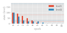
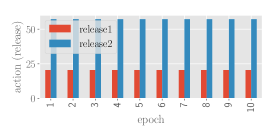
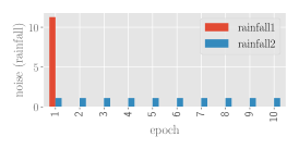
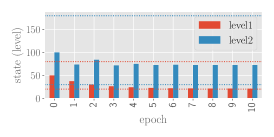
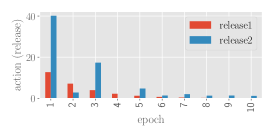
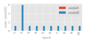
Figure 5: Worst-case state trajectory (left col.), actions (middle col.), and disturbances/noise (right col.) for C (top row) and S policies (bottom row) computed by Algorithm 1 for the reservoir control problem.

Worst-Case Analysis

Fig. 5 plots the state trajectory, actions and noise (i.e. rainfall) that lead to worst-case performance of C and S policies after the last iteration of Algorithm 1 for reservoir. Here, we observe that the worst-case performance for the optimal constant-value (C) policy occurs when the rainfall is low and both reservoirs become empty. Given that the cost of overflow exceeds underflow, this is expected as the C policy must release enough water to prevent high-cost overflow events during high rainfall at the risk of water shortages during droughts – this scenario results in non-zero cost and is identified by CGPO as incurring the worst-case cumulative reward in this policy class. In contrast, the optimal linear-valued (S) policy maintains safe water levels even in the worst-case scenario, since it can avoid underflow and overflow events by assigning release amounts that increase linearly with the water levels.

Analysis of Problem Size

To understand how the problem sizes in CGPO scale across differing expressivity classes of policies and dynamics, Table 2 shows the number of decision variables and constraints in the MIPs at the last iteration of constraint generation (more details are provided as supplementary material). For VTOL with a quadratic (Q) policy, the number of variables in the inner and outer problems are 0 / 0 / 212 and 0 / 0 / 512, resp., while the number of constraints are 114 / 18 / 72 and 270 / 95 / 155. The number of decision variables/constraints are fixed in the inner problem and grow linearly with iterations in the outer problem. Fortunately, the number of variables and constraints do not grow significantly with the expressiveness of the policy class.

Conclusion

We presented a novel bi-level mixed-integer programming formulation for DC-MDP policy optimization in predefined expressivity classes with bounded optimality guarantees. Constraint generation allowed us to decompose this into an inner problem that produces an adversarial worst-case constraint violation (i.e., trajectory), and an outer problem that improves the policy w.r.t. the most violated constraints. The result is our novel constraint generation policy optimization (CGPO) algorithm. Using inventory, reservoir and VTOL control problems, we demonstrated that the policies learned and their worst-case performance/failure modes were easy to interpret, while maintaining a manageable number of variables and constraints in the corresponding MIPs.

Appendix

Proof of Theorem 1

In the notation of Blankenship and Falk (1976), we define $X^{0}=[0,2BT]$, $X=\mathcal{W}$, $Y=\mathcal{A}^{T}\times\mathcal{S}_{1}\times\Xi_{p}^{T}$. Making the change of variable $\varepsilon=x_{0}\in X^{0}$, $x=\mathbf{w}$, and $y=(\alpha,\mathbf{s}_{1},\xi_{1:T})\in Y$, and defining the continuous function $f(x,y)=\varepsilon(\alpha,\mathbf{s}_{1},\xi_{1:T})=V(\alpha,\mathbf{s}_{1},\xi_{1:T})-V(\mathbf{w},\mathbf{s}_{1},\xi_{1:T})$, the problem (8) is equivalent to the problem:

$$\min_{(x_{0},x)\in X^{0}\times X} \,x_{0}$$

$$\mathrm{s.t.} \,f(x,y)-x_{0}\leq 0,\quad\forall y\in Y$$

as discussed on p. 262 of Blankenship and Falk (1976). Similarly, our Algorithm 1 is a special case of the Algorithm 2.1 in the aforementioned paper, specialized to the problem state, with $x_{t}=\mathbf{w}_{t}^{*}$. Thus, the assumption of Theorem 2.1 in Blankenship and Falk (1976) holds, and $\mathbf{w}_{t}^{*}$ is a solution of (8) as claimed. $\square$

Further Remarks About Theorem 1

In general, Algorithm 1 may not necessarily terminate, unless much stronger convexity requirements are placed on $V(\alpha,\mathbf{s})$ and $V(\mathbf{w},\mathbf{s})$, and potentially the class of MDPs solved. Thus, in a typical application, one can instead monitor the solution differences $\|\mathbf{w}_{t}^{*}-\mathbf{w}_{t-1}^{*}\|$, and terminate with an approximate solution when this difference is sufficiently small. However, our experiments run a fixed number of iterations, showing empirically that Algorithm 1 does indeed terminate on all problems with an exact optimal solution for most policy classes considered, at which point both the return and error curves “plateau” (cf. Figure 4).

Domains

Here we provide more complete mathematical descriptions of the benchmark problems used in the experiments. In what follows, we define $(\cdot)_{+}=\max[0,\cdot]$.

Linear Inventory

The state transition model can be written as:

$$s_{t+1} =s_{t}+a_{t}-\xi_{t},\quad\xi_{t}\sim\lfloor\mathrm{Uniform}(L,U)\rfloor,$$

s.t. $$0\leq a_{t}\leq B,\quad\forall t.$$

We define costs $C,P$ and $S$ which represent, respectively, the purchase cost, excess inventory cost and shortage cost. The reward function can thus be written as

$$r(\mathbf{s}_{t+1}) =-C\times a_{t}-P\times(s_{t+1})_{+}-S\times(-s_{t+1})_{+}.$$

We set $B=10$, $C=0.5$, $P=S=2$, $L=2$, $U=6$. If $P>C$ and $T=\infty$, then a PWS-S policy is provably optimal (otherwise if $T<\infty$, then it may be non-stationary).

Linear Reservoir

Let $s_{t,r}$ denote the water level of reservoir $r$, $a_{t,r}$ be the amount of water to release from reservoir $r$, $\xi_{t,r}$ denote the stochastic rainfall amount affecting reservoir $r$, $U(r)$ denote the set of upstream reservoirs connected to reservoir $r$, and $M_{r}$ be the maximum capacity of reservoir $r$. The state transition model can be written as:

$$s_{t+1,r} =\min\Big{[}M_{r},\Big{(}s_{t,r}+(\xi_{t,r})_{+}-a_{t,r}+\sum_{d\in U(r)}a_{t,d}\Big{)}_{+}\Big{]},$$

$$\xi_{t,r} \sim\mathrm{Normal}(m_{r},v_{r}),$$

s.t. $$0\leq a_{t,r}\leq s_{t,r},\quad\forall t,r.$$

The goal is to maintain the level of water within target range $[L_{r},H_{r}]$. Penalties $l_{r}$ and $h_{r}$ are assigned for any quantity of water above or below the required target level. Thus, the reward function can be written as

$$r(\mathbf{s}_{t+1}) =\sum_{r=1}^{N}l_{r}(L_{r}-s_{t+1,r})_{+}+h_{r}(s_{t+1,r}-H_{r})_{+}.$$

Our experiment uses a two-reservoir system with the following values for reservoir 1 $L_{1}=20,H_{1}=80,M_{1}=100,m_{1}=5,v_{1}=5,U(1)=\emptyset$, and the following values for reservoir 2 $L_{2}=30,H_{2}=180,M_{2}=200,m_{2}=10,v_{2}=10,U(2)=\{1\}$. Costs are shared and set to $l_{r}=-10,h_{r}=-100$.

Nonlinear VTOL Control

The state dynamics evolve according to:

$$\theta_{t+1} =\max\left[-\sin(h/l_{1}),\min\left[\sin(h/l_{2}),\theta_{t}+\tau\omega_{t}\right]\right]$$

$$\omega_{t+1} =\omega_{t}+\frac{\tau}{J}\left(9.8(m_{2}l_{2}-m_{1}l_{1})\cos\theta_{t}+150l_{1}F_{t}\right)$$

$$J =m_{1}l_{1}^{2}+m_{2}l_{2}^{2}$$

s.t. $$l_{1}m_{1}\geq l_{2}m_{2},\quad l_{1}>l_{2}>h,\quad 0\leq F_{t}\leq 1.$$

The reward is defined as the negative absolute difference between the angle at each epoch and the target angle $\theta_{target}=0$, i.e.

$$r(F_{t},\theta_{t+1},\omega_{t+1})=-|\theta_{t+1}-\theta_{target}|.$$

We use values $l_{1}=1,l_{2}=0.5,m_{1}=10,m_{2}=1,h=0.4,g=9.8$.

Quadratic policies are of the form

$$F(\theta_{t},\omega_{t})=w_{0}+w_{1}\theta_{t}+w_{2}\omega_{t}+w_{3}\theta_{t}\omega_{t}+w_{4}\theta_{t}^{2}+w_{5}\omega_{t}^{2},$$

where $w_{i}$ are bounded in $[-100,100]$. Since coefficients are allowed to be both positive and negative, this increases the expressivity of the policy class at the expense of potentially inducing non-convexity of the objective.

Nonlinear Intercept

The intercept problem is a nonlinear domain with Boolean actions. It involves two objects moving in continuous trajectories in a subset of $\mathbb{R}^{2}$, in which one object (e.g. missile, bird) flies in a parabolic arc across space towards the ground, and must be intercepted by a second object (e.g. anti-ballistic missile, predator) that is fired from a fixed position on the ground. While the problem is best described in continuous time, we study a discrete-time version of the problem. The state includes the position $(x_{t},y_{t})$ of the missile at each decision epoch, as well as “work” variables indicating whether the interceptor has already been fired $f_{t}$ as well as its vertical elevation $i_{t}$. Meanwhile, the action $a_{t}$ is Boolean-valued and indicates whether the interceptor is fired at a given time instant.

The state transition model can be written as:

$$x_{t+1} =x_{t}+v_{x},\quad y_{t+1}=h-\frac{1}{2}gx_{t}^{2}$$

$$f_{t+1} =f_{t}\lor a_{t},\quad i_{t+1}=\begin{cases}i_{t}&\mbox{ if }f_{t}=0\\ i_{t}+v_{y}&\mbox{ if }f_{t}=1\end{cases},$$

ignoring the gravitational interaction of the interceptor. Interception happens whenever the absolute differences between the coordinates of the missile and the interceptor are within $\delta$, so the reward is

$$r(s_{t+1})=\begin{cases}1&\mbox{ if }f_{t+1}\land|x_{t+1}-i_{x}|\leq\delta\land|y_{t+1}-i_{t+1}|\leq\delta\\ 0&\mbox{ otherwise}\end{cases}.$$

We set $v_{x}=0.1,h=5,g=9.8,i_{x}=0.7$.

We study Boolean-valued policies with linear constraints (i.e., B, PWL-B) that take into account the position of the missile at each epoch, i.e. PWL1-B policies of the form

$$a_{t}(x_{t},y_{t})=\begin{cases}a_{1}&\mbox{ if }l\leq w_{1}x_{t}+w_{2}y_{t}\leq u\\ a_{2}&\mbox{ otherwise}\end{cases}$$

where $a_{1},a_{2}\in\{0,1\}$ and $l,u,w_{1},w_{2}$ are all tunable parameters.

Domain RDDL Descriptions

RDDL domain descriptions of the above problems are provided as accompaniment to the supplementary material.

Initial State Bounds $\mathcal{S}_{1}$

For reservoir and inventory control, bounds on the initial state have been chosen as intervals centred on the initial state specified in the RDDL domain description. For reservoir control, these bounds are intervals centred around the initial state $(75,150)$, i.e. $[50,100]$ for reservoir 1 and $[100,200]$ for reservoir 2. For inventory control, the bounds are $[0,2]$, for VTOL they are fixed to the initial state of the system $\theta=0.1,\omega=0$, and for intercept they are also fixed to the initial state $x=0,y=5,f=0,i=0$.

Gurobi and Environment Settings

We use the Python implementation of the Gurobi Optimizer (GurobiPy) version 10.0.1, build v10.0.1rc0 for Windows 64-bit systems, with an academic license. Default optimizer settings have been used, with the exception of NumericFocus set to 2 in order to enforce numerical stability, and the MIPGap parameter set to 0.05 to terminate when the optimality gap reaches 5%. All experiments were conducted on a single machine with an Intel 10875 processor (base at 2.3 GHz, overclocked at 5.1 GHz) and 32 GB of RAM.

Additional Implementation Details

Action Constraints

One important issue concerns how to enforce constraints on valid actions. Two valid approaches include (1) explicitly constraining actions in RDDL constraints (state invariants and action preconditions) by compiling them as MIP constraints, or (2) implicitly clipping actions in the state dynamics (conditional probability functions in RDDL). Crucially, we found the latter approach performed better during optimization, since constraining actions inherently limits the policy class to a subset of weights that can only produce legal actions across the initial state space. This not only significantly restricts policies (i.e. for linear valued policies, the weights would be constrained to a tight subset where the output for every possible state would be a valid action) but also poses challenges for the optimization process, which is significantly complicated by these action constraints.

Handling Numerical Errors

Mathematical operations, such as strict inequalities, cannot be handled explicitly in Gurobi. To perform accurate translation of such operations in our code-base, we used indicator/binary variables. For instance, to model the comparison $a>b$ for two numerical values $a,b$, we define a binary variable $y\in\{0,1\}$ and error parameter $\epsilon>0$ constrained as follows:

$$y==1 \implies a\geq b+\epsilon$$

$$y==0 \implies a\leq b.$$

In practice, $\epsilon$ is typically set larger than the smallest positive floating point number in Gurobi (around $10^{-5}$), but is often problem-dependent. We derived optimal policies for all domains using $\epsilon=10^{-5}$, except Intercept where we needed to use a larger value of $\epsilon=10^{-3}$ to allow Gurobi to correctly distinguish between the two cases above.

Additional Experimental Results

Intercept

Fig. 6 illustrates the return and worst-case error of Boolean-valued policies for the intercept problem. Only the policies with at least one case are optimal, with corresponding error of zero. As illustrated in the last plot in Fig. 7, the optimal policies fire whenever a threat is detected in the top right corner of the airspace.

Policy Representations

Fig. 8 and Fig. 9 showcase policies learned in other expressivity classes besides those shown in the main text, for inventory and reservoir control, respectively. Fig. 7 illustrates the policies for the intercept problem. As can be seen, policies generally remain intuitive and easy to explain even as the complexity increases. For instance, PWS2-C policies for inventory control order more inventory as the stock level decreases, while the amount of water released is increasing in the water level for reservoir control. Interestingly, the PWS2-C policies for inventory control and the intercept problem contain redundant constraints.

Worst-Case Analysis

Fig. 10 and Fig. 11 illustrate worst case scenarios induced by the C and S policies for inventory and VTOL control, respectively. Similar to reservoir control, a non-trivial worst-case scenario is identified by CGPO for inventory control for optimal C policies but not S policies. This scenario corresponds to very high demand that exceeds the constant reorder quantity, causing stock-outs. For the VTOL control problem, there is no worst-case scenario with non-zero cost upon convergence at the final iteration of CGPO (bottom row). We have also shown the worst-case scenario computed at the first iteration prior to achieving policy optimality, where a worst-case scenario corresponds to no force being applied causing the system to eventually lose balance. The ability to interpret the worst-case scenario prior to convergence, or if convergence cannot be achieved, could help to decide whether the policy is trustworthy, and how to prepare for the worst-case if the policy is deployed in practice.

Analysis of Problem Size

Fig. 12, Fig. 13 and Fig. 14 summarize the total number of variables and constraints in the outer MIP formulations solved by CGPO at each iteration for inventory, reservoir and VTOL control, respectively. Each iteration of constraint generation requires a roll-out from the dynamics and reward model, which in turn requires instantiate a new set of variables to hold the intermediate state and reward computations, and thus the number of variables and constraints grows linearly with the iterations. Even at the last iteration of CGPO, we see that the number of variables and constraints remains manageable.

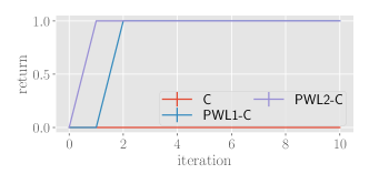
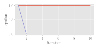
Figure 6: Simulated return (left) and optimal value of $\varepsilon^{*}$ (right) as a function of the number of iterations of constraint generation for the intercept domain.

$fire=1$

$fire=\begin{cases}0&\mbox{ if }-0.136\leq-0.2x-0.02y\leq 0\\ 1&\mbox{ otherwise}\end{cases}$

$fire=\begin{cases}0&\mbox{ if }-0.136\leq-0.2x-0.02y\leq 0\\ 0&\mbox{ if }0.001\leq-x\leq 1\\ 1&\mbox{ otherwise}\end{cases}$

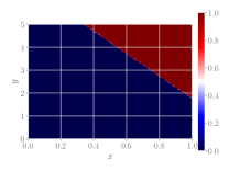
Figure 7: From left to right, examples of learned B, PWS1-B and PWS2-B policies and visualization of PWS-B policy for the intercept problem.

$order=3$

$order=4-stock$

$order=\begin{cases}8&\mbox{ if }-13\leq stock\leq-2\\ 2&\mbox{ otherwise}\end{cases}$

$order=\begin{cases}6&\mbox{ if }-10\leq stock\leq-1\\ 1&\mbox{ if }2\leq stock\leq 2\\ 3&\mbox{ otherwise}\end{cases}$

Figure 8: From left to right, examples of learned C, S, PWS1-C and PWS2-C policies for the inventory control problem.

$release_{1}=19.73$ $release_{2}=55.87$

$release_{1}=level_{1}-20$ $release_{2}=0.93\times level_{2}-29.74$

$release_{1}=\begin{cases}1.39&\mbox{ if }30.62\leq level_{1}\leq 68.66\\ 40.71&\mbox{ if }70.93\leq level_{1}\leq 100\\ 10.622&\mbox{ otherwise}\end{cases}$ $release_{2}=\begin{cases}80.78&\mbox{ if }159.93\leq level_{2}\leq 200\\ 38.69&\mbox{ if }144.21\leq level_{2}\leq 159.11\\ 18.25&\mbox{ otherwise}\end{cases}$

$release_{1}=\begin{cases}level_{1}-50&\mbox{ if }20\leq level_{1}\leq 100\\ 2\times level_{1}-100&\mbox{ otherwise}\end{cases}$ $release_{2}=\begin{cases}level-2-37.8&\mbox{ if }38.9\leq level_{2}\leq 200\\ 1.17\times level_{2}-235.5&\mbox{ otherwise}\end{cases}$

Figure 9: From left to right, examples of learned C, S, PWS2-C and PS1-S policies for the reservoir control problem.

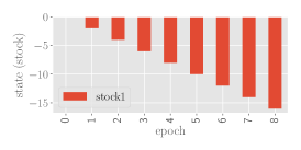
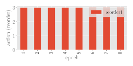
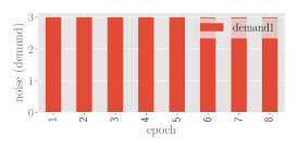
Figure 10: Worst-case state trajectory (left col.), actions (middle col.), and disturbances/noise (right col.) for C (top row) and S policies (bottom row) computed by Algorithm 1 for the inventory control problem.

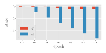
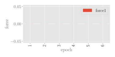
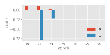
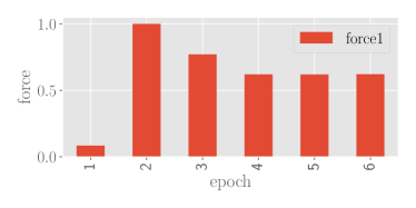
Figure 11: For VTOL control, worst-case state trajectory (top row), and actions $\mathbf{a}_{1}^{*},\dots\mathbf{a}_{T}^{*}$ (bottom row) for Q policies. First (last) column corresponds to the first (last) iterations of Algorithm 1.

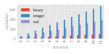
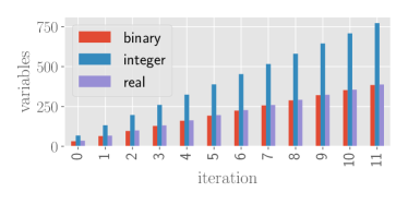
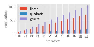
Figure 12: Number of decision variables (left) and constraints (right) for C policy (top row) and PWS1-S policy (bottom row) corresponding to the outer optimization problem at each iteration applied to the inventory problem.

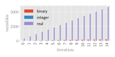
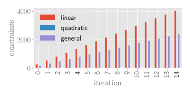
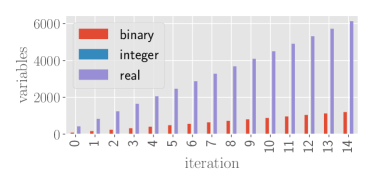
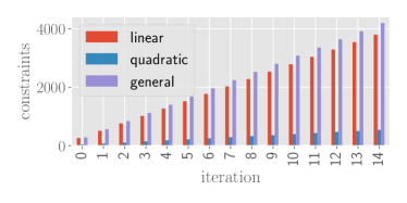
Figure 13: Number of decision variables (left) and constraints (right) for C policy (top row) and PWS1-S policy (bottom row) corresponding to the outer optimization problem at each iteration applied to the reservoir problem.

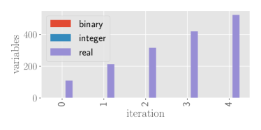
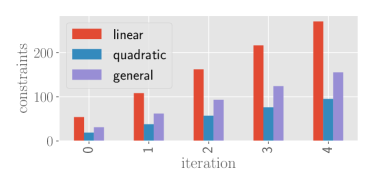
Figure 14: Number of decision variables (left) and constraints (right) for Q policy corresponding to the outer optimization problem at each iteration applied to the VTOL problem.

References

- Albert (2022) Albert, L. A. 2022. A mixed-integer programming model for identifying intuitive ambulance dispatching policies. Journal of the Operational Research Society, 1–12.
- Ariu et al. (2017) Ariu, K.; Fang, C.; da Silva Arantes, M.; Toledo, C.; and Williams, B. C. 2017. Chance-Constrained Path Planning with Continuous Time Safety Guarantees. In AAAI Workshop.
- Åström (2012) Åström, K. J. 2012. Introduction to stochastic control theory. Courier Corporation.
- Blankenship and Falk (1976) Blankenship, J. W.; and Falk, J. E. 1976. Infinitely constrained optimization problems. Journal of Optimization Theory and Applications, 19: 261–281.
- Boutilier, Reiter, and Price (2001) Boutilier, C.; Reiter, R.; and Price, B. 2001. Symbolic dynamic programming for first-order MDPs. In IJCAI, volume 1, 690–700.
- Bueno et al. (2019) Bueno, T. P.; de Barros, L. N.; Mauá, D. D.; and Sanner, S. 2019. Deep reactive policies for planning in stochastic nonlinear domains. In AAAI, volume 33, 7530–7537.
- Castro (2015) Castro, P. M. 2015. Tightening piecewise McCormick relaxations for bilinear problems. Computers & Chemical Engineering, 72: 300–311.
- Chembu et al. (2023) Chembu, A.; Sanner, S.; Khurram, H.; and Kumar, A. 2023. Scalable and Globally Optimal Generalized L1 k-center Clustering via Constraint Generation in Mixed Integer Linear Programming. In AAAI, volume 37, 7015–7023.
- Corso et al. (2021) Corso, A.; Moss, R.; Koren, M.; Lee, R.; and Kochenderfer, M. 2021. A survey of algorithms for black-box safety validation of cyber-physical systems. Journal of Artificial Intelligence Research, 72: 377–428.
- Farina, Giulioni, and Scattolini (2016) Farina, M.; Giulioni, L.; and Scattolini, R. 2016. Stochastic linear model predictive control with chance constraints–a review. Journal of Process Control, 44: 53–67.
- Feng and Hansen (2002) Feng, Z.; and Hansen, E. A. 2002. Symbolic heuristic search for factored Markov decision processes. In AAAI, 455–460.
- Gurobi Optimization, LLC (2023) Gurobi Optimization, LLC. 2023. Gurobi Optimizer Reference Manual.
- Hickey, Ju, and Van Emden (2001) Hickey, T.; Ju, Q.; and Van Emden, M. H. 2001. Interval arithmetic: From principles to implementation. Journal of the ACM, 48(5): 1038–1068.
- Keller and Eyerich (2012) Keller, T.; and Eyerich, P. 2012. PROST: Probabilistic planning based on UCT. In ICAPS, volume 22, 119–127.
- Kleywegt, Shapiro, and Homem-de Mello (2002) Kleywegt, A. J.; Shapiro, A.; and Homem-de Mello, T. 2002. The sample average approximation method for stochastic discrete optimization. SIAM Journal on optimization, 12(2): 479–502.
- Low, Kumar, and Sanner (2022) Low, S. M.; Kumar, A.; and Sanner, S. 2022. Sample-Efficient Iterative Lower Bound Optimization of Deep Reactive Policies for Planning in Continuous MDPs. In AAAI, volume 36, 9840–9848.
- Morrison et al. (2016) Morrison, D. R.; Jacobson, S. H.; Sauppe, J. J.; and Sewell, E. C. 2016. Branch-and-bound algorithms: A survey of recent advances in searching, branching, and pruning. Discrete Optimization, 19: 79–102.
- Ono et al. (2015) Ono, M.; Pavone, M.; Kuwata, Y.; and Balaram, J. 2015. Chance-constrained dynamic programming with application to risk-aware robotic space exploration. Autonomous Robots, 39: 555–571.
- Poupart and Boutilier (2003) Poupart, P.; and Boutilier, C. 2003. Bounded Finite State Controllers. In NeurIPS, 823–830.
- Puterman (2014) Puterman, M. L. 2014. Markov decision processes: discrete stochastic dynamic programming. John Wiley & Sons.
- Raghavan et al. (2012) Raghavan, A.; Joshi, S.; Fern, A.; Tadepalli, P.; and Khardon, R. 2012. Planning in factored action spaces with symbolic dynamic programming. In AAAI, volume 26, 1802–1808.
- Raghavan et al. (2017) Raghavan, A.; Sanner, S.; Khardon, R.; Tadepalli, P.; and Fern, A. 2017. Hindsight optimization for hybrid state and action MDPs. In AAAI, volume 31.
- Sanner (2010) Sanner, S. 2010. Relational dynamic influence diagram language (rddl): Language description. Unpublished ms. Australian National University, 32: 27.
- Sanner, Delgado, and de Barros (2011) Sanner, S.; Delgado, K. V.; and de Barros, L. N. 2011. Symbolic dynamic programming for discrete and continuous state MDPs. In AAAI, 643–652.
- Say et al. (2017) Say, B.; Wu, G.; Zhou, Y. Q.; and Sanner, S. 2017. Nonlinear hybrid planning with deep net learned transition models and mixed-integer linear programming. In IJCAI, 750–756.
- Scala et al. (2016) Scala, E.; Haslum, P.; Thiébaux, S.; and Ramirez, M. 2016. Interval-based relaxation for general numeric planning. In ECAI, 655–663. IOS Press.
- Scarf et al. (1960) Scarf, H.; Arrow, K.; Karlin, S.; and Suppes, P. 1960. The optimality of (S, s) policies in the dynamic inventory problem. Optimal pricing, inflation, and the cost of price adjustment, 49–56.
- Świechowski et al. (2023) Świechowski, M.; Godlewski, K.; Sawicki, B.; and Mańdziuk, J. 2023. Monte Carlo tree search: A review of recent modifications and applications. Artificial Intelligence Review, 56(3): 2497–2562.
- Taitler et al. (2022) Taitler, A.; Gimelfarb, M.; Gopalakrishnan, S.; Mladenov, M.; Liu, X.; and Sanner, S. 2022. pyRDDLGym: From RDDL to Gym Environments. arXiv preprint arXiv:2211.05939.
- Topin et al. (2021) Topin, N.; Milani, S.; Fang, F.; and Veloso, M. 2021. Iterative bounding mdps: Learning interpretable policies via non-interpretable methods. In AAAI, volume 35, 9923–9931.
- Vos and Verwer (2023) Vos, D.; and Verwer, S. 2023. Optimal Decision Tree Policies for Markov Decision Processes. arXiv preprint arXiv:2301.13185.
- Wang et al. (2022) Wang, Y.; Wang, J.; Zhang, W.; Zhan, Y.; Guo, S.; Zheng, Q.; and Wang, X. 2022. A survey on deploying mobile deep learning applications: A systemic and technical perspective. Digital Communications and Networks, 8(1): 1–17.
- Wu, Say, and Sanner (2017) Wu, G.; Say, B.; and Sanner, S. 2017. Scalable planning with tensorflow for hybrid nonlinear domains. NeurIPS, 30.
- Zamani, Sanner, and Fang (2012) Zamani, Z.; Sanner, S.; and Fang, C. 2012. Symbolic dynamic programming for continuous state and action mdps. In AAAI, volume 26, 1839–1845.