A distribution-guided Mapper algorithm

Abstract

Motivation: The Mapper algorithm is an essential tool to explore shape of data in topology data analysis. With a dataset as an input, the Mapper algorithm outputs a graph representing the topological features of the whole dataset. This graph is often regarded as an approximation of a reeb graph of data. The classic Mapper algorithm uses fixed interval lengths and overlapping ratios, which might fail to reveal subtle features of data, especially when the underlying structure is complex.
Results: In this work, we introduce a distribution guided Mapper algorithm named D-Mapper, that utilizes the property of the probability model and data intrinsic characteristics to generate density guided covers and provides enhanced topological features. Our proposed algorithm is a probabilistic model-based approach, which could serve as an alternative to non-prababilistic ones. Moreover, we introduce a metric accounting for both the quality of overlap clustering and extended persistence homology to measure the performance of Mapper type algorithm. Our numerical experiments indicate that the D-Mapper outperforms the classical Mapper algorithm in various scenarios. We also apply the D-Mapper to a SARS-COV-2 coronavirus RNA sequences dataset to explore the topological structure of different virus variants. The results indicate that the D-Mapper algorithm can reveal both vertical and horizontal evolution processes of the viruses.
Availability: Our package is available at https://github.com/ShufeiGe/D-Mapper.
Contact: geshf@shanghaitech.edu.cn

1 Introduction

In recent decades, machine learning methods have become popular tools to discover valuable information from data. These methods typically focus on prediction tasks by establishing a mapping between responses and predictors. The shape of data may reveal important information in data from a new perspective and provide alternative insights to supplement prediction tasks, which is often overlooked in the learning of mapping. To be specific, the shape of data refers to the manifold formed by the support set of data distribution. The shape of data reveals the data distribution, reflecting the spatial correlations and dependency structures among data points. Such information is crucial in clustering and feature extraction tasks. However, many existing methods cannot fully utilize such information.

Topology data analysis (TDA) is a specific area of investigating data shapes based on topological theory. Topology is a powerful tool to study the shape of objects by finding invariants that remain unchanged under continuous deformations. These invariants can reflect objects’ intrinsic features. TDA attempts to identify and utilize these topology invariants in data analysis. The Mapper algorithm is a simple but powerful TDA tool for visualizing and clustering data. The algorithm constructs a graph in which each vertex represents a cluster, and each edge represents the two adjacent clusters that share some elements. The colour and size of vertices are defined by users and can provide more information. The size of vertices and the colour depth can represent the average value and the number of elements in the cluster. The Mapper algorithm was first proposed in singhTopologicalMethodsAnalysis and has been applied in various domains, such as social media almgrenMiningSocialMedia2017 , fraud detection mitraExperimentsFraudDetection2021 , and evolutionary computation todaVisualizationClusteringGraph2022 . The Mapper algorithm is especially suitable for biology data, which are usually complex and high-dimensional skafTopologicalDataAnalysis2022 . For example, the Mapper algorithm was applied to breast cancer transcriptional microarray data and successfully identified two subgroups with $100\%$ survival rate nicolauTopologyBasedData2011 . It is also used to analyze transcriptional programs that control cellular lineage commitment and differentiation during development, and the proposed scTDA identified four transient states over time rizviSinglecellTopologicalRNAseq2017 . Exploring the conformation space of proteins is another important task in computational biology, and the Mapper algorithm has been successfully applied to analyze intermediate conformations, the results are closely consistent with experimental findings dehghanpoorUsingTopologicalData .

The classic Mapper algorithm requires to select a filter function $f:X\rightarrow\mathbb{R}^{n}$ that projects data $X$ onto the Euclidean space $\mathbb{R}^{n}$ and a set of open cover $\mathcal{U}$ on the projection data. Different filter functions and open covers may result in different outputs, so it is necessary to select them carefully. Improper filter functions or open covers may not accurately reveal data shapes, resulting in poor overlap clustering. A filter function is chosen primarily based on features of interest and also depends on specific applications. Determining the optimal parameters of the model, such as the overlapping rates and interval lengths, usually requires extensive manual tuning and experiments. As pointed out in carriereStatisticalAnalysisParameter2017 , cover choices lead to a broad range of possible Mapper outputs, resulting in many different graph depictions and clustering results. Unreasonable choices may cause the disappearance of certain topological features.

Many works were proposed to improve the performance of the classic Mapper. For example, dlotkoBallMapperShape2019 proposed to generate covers on the dataset by constructing a set of balls directly. This method saved trouble of choosing filter function. buiFMapperFuzzyMapper2020 used fuzzy clustering algorithm to generate covers to choose cover automatically with random overlap ratios. To achieve adaptive cover construction, a information criteria was developed based on X-means algorithm to generate adaptive covers chalapathiAdaptiveCoversMapper2021 .

In this work, alternatively, we propose a distribution-guided Mapper algorithm to relax the restriction of regular covers and overlapping. Our proposed algorithm utilizes the property of the probability model and data intrinsic characteristics to generate distribution guided covers and provides enhanced topological features. Our proposed algorithm is a probabilistic model-based approach, which could serve as an alternative to non-probabilistic ones. Unlike the classic Mapper algorithm, our proposed D-Mapper does not rely on predefined static overlap rates and interval lengths, but instead we fit projected data to a mixture distribution model and generate flexible covers automatically. Moreover, the performance of Mapper algorithm is hard to evaluate due to the complexity of output graph structure, most of literature only evaluate from the clustering perspective buiFMapperFuzzyMapper2020 ; chalapathiAdaptiveCoversMapper2021 , however these method overlooks the quality of topological structure. In this paper, We introduce a metric that can quantitatively and objectively evaluate the performance of Mapper algorithm from both clustering and topological aspects. We use the extended persistence homology as a tool to capture topological signatures, then we distinguish noise and signal on the diagram by constructing confidence set on the diagram, the signal rate can be a metric to evaluate the quality of topological structure. All the simulation and application studies indicate that the D-Mapper algorithm outperforms the classic Mapper algorithm. The reminder of the paper is organized as follows. We briefly review the classic Mapper algorithm and introduce our D-Mapper and evaluation metric in the Materials and methods. Simulation section focuses on the comparison of the classic Mapper and the D-Mapper on simulated datasets. In Application section, we applied D-Mapper algorithm on a real world SARS-COV-2 RNA sequences dataset. We summarize our work and discuss the future work in the conclusion section.

2 Materials and methods

2.1 Basic notions

Before we introduce our method, we first briefly review the essential background of the Mapper algorithm. The theoretical foundation of the Mapper algorithm is the Nerve theorem which guarantees the nerves produced by a cover on a topology space $X$ is homomorphic equivalent to that space. We introduce the following notions to describe Nerve theorem carlssonTopologyData2009 ; chazalIntroductionTopologicalData2021 .

Definition 1 (Simplex).

Given a set $P=\{p_{0},...,p_{k}\}\subset\mathbb{R}^{n}$ of k+1 affinely independent points, a $k$-dimensional simplex $\sigma$, or $k$-simplex for short, spanned by $P$ is the set of convex combinations such that:

$$\{x|x=\sum_{i=0}^{k}\lambda_{i}p_{i},\sum_{i=0}^{k}\lambda_{i}=1,\lambda_{i}\geq 0\}.$$

And the points of $P$ are the vertices of simplex $\sigma$ and the simplices spanned by the subsets of P are the faces of simplex $\sigma$.

Definition 2 (Geometric simplicial complex).

A geometric simplicial complex $K$ in $\mathbb{R}^{n}$ is a finite collection of simplices satisfying the following two conditions:
a) Arbitrary face of any simplex of $K$ is a simplex of $K$.
b) The intersection of any two simplices of $K$ is either empty or the common face of the two.

The union of the simplices of $K$ constitutes the underlying space of $K$, denoted as $|K|$, which inherits from the topology of $\mathbb{R}^{n}$. Thus the geometric simplicial complex can also be regarded as a topology space.

Definition 3 (Abstract simplicial complex).

Let $V$ be a finite set. An abstract simplicial complex $\mathcal{K}$ given the set $V$ is a set of finite subsets of $V$ such that:
a) All elements of $V$ belongs to $\mathcal{K}$.
b) If $\tau\in\mathcal{K}$ , any subset of $\tau$ belongs to $\mathcal{K}$.

Definition 4 (Open cover).

Suppose $\mathcal{U}=(u_{i}),i\in I$ is a collection of open subset of a topological space $X$, then we say $\mathcal{U}$ is an open cover of $X$ if $X\subset\bigcup_{i\in I}u_{i}$.

Given an open cover of topological space $X$, $\mathcal{U}=(u_{i})$, the nerve of $\mathcal{U}$ is an abstract simplicial complex C$(\mathcal{U})$ with vertex set $\mathcal{U}$. With these definitions, we can introduce the most important theorem in constructing Mapper.

Theorem 1 (Nerve Theorem).

Let $\mathcal{U}=(u_{i}),i\in I$ be a cover of a topological space $X$ by open sets such that the intersection of any sub-collection of the $u_{i}$’s is either empty or contractible. Then, $X$ and the nerve C($\mathcal{U}$) are homotopy equivalent.

This theorem allows us to map the topology of continuous into abstract combinatorial structures by building a nerve complex. It bridges the gap between continuous space and its discrete representation. Many TDA methods, including the Mapper algorithm, are built based on this crucial theorem.

2.2 Mapper algorithm

Mapper algorithm is an important tool to construct the discrete version of reeb graphs which encode connected information of the support manifold deyTopologicalAnalysisNerves2017 . Algorithm 1 depicts the classic Mapper algorithm. Firstly, the original data is projected onto a real line by a user-specified filter function (Algorithm 1, line 1). To construct a cover $\mathcal{U}$ on the projected data, the number of components $n$ and overlap ratio $p$ should be chosen carefully (Algorithm 1, line 2). The improper choice of these parameters may lead to failure estimation of the shape of data. With these two parameters, a cover with $n$ regular intervals can be obtained (Algorithm 1, line 3). Then, the inverse image of the cover $\mathcal{U}$ is achieved on the original data, generating some hypercubes. This process is often called pulling back (Algorithm 1, line 4). Finally, clustering data points within each hypercubes. Each cluster corresponds to a vertex in the Mapper graph. If two vertexes share any elements, an edge is added between these two vertices (Algorithm 1, line 5).

Algorithm 1 The classic Mapper Algorithm

1:Choose a proper filter function $f$ to project data on the real line, $f:X\rightarrow\mathbb{R}$.

2:Choose a component number $n$ and overlap percentage ratio $p$.

3:Construct a cover $\mathcal{U}=(u_{i}),i=1...n$ on projected data $f(X)$ based on the parameter $n$ and $p$.

4:Pull back the intervals of projected data, $f^{-1}(\mathcal{U})$.

5:Cluster on the refined cover and build the nerves with the clustering result.

The Mapper algorithm is powerful for exploring and visualizing data, while the selection of parameters $n,~{}p$ involves extensive manual tuning and the algorithm is sensitive to these parameters. In addition, the Mapper algorithm’s flexibility is often restricted by regular intervals and fixed overlap ratios, which may hinder the discovery of complex data structures.

2.3 D-Mapper

The restriction of regular intervals with fixed overlap ratios is one of the major limitations of the Mapper algorithm. We propose a distribution-guided Mapper algorithm to generate flexible covers to reflect the underlying data structures. Our proposed method automatically chooses the overlap ratios based on the distribution of the projection data and produces more flexible covers to reveal the data shapes more accurately. Our experiments indicate that our method produces better results than the classic Mapper algorithm in terms of clustering. The key idea of our algorithm is to fit projected data with a mixture model. Each component in the mixture model can be viewed as a cluster, and the probability (likelihood) of each data point assigned to each cluster can be explicitly calculated. Once we get the mixture distribution of projected data, we can create intervals base on the distribution in many ways.

Here we introduce a simply way to construct intervals based on the quantile $\alpha$ of the probability distribution. With proper selection, the $\alpha$ quantile interval of each component of the mixture model can automatically produce some overlaps, Figure 1 shows the idea of naturally producing intervals by quantile $\alpha$. This attribute provides a natural scheme for constructing flexible covers on projected data. The specific procedures are as follows:
1) Choose an appropriate number of intervals $n$ and a quantile $\alpha$. The number of components naturally matches the number of intervals.
2) Use a mixture model to fit the projected data.
3) Intervals are determined by the $\alpha$ quantile intervals of each component of the mixture model.

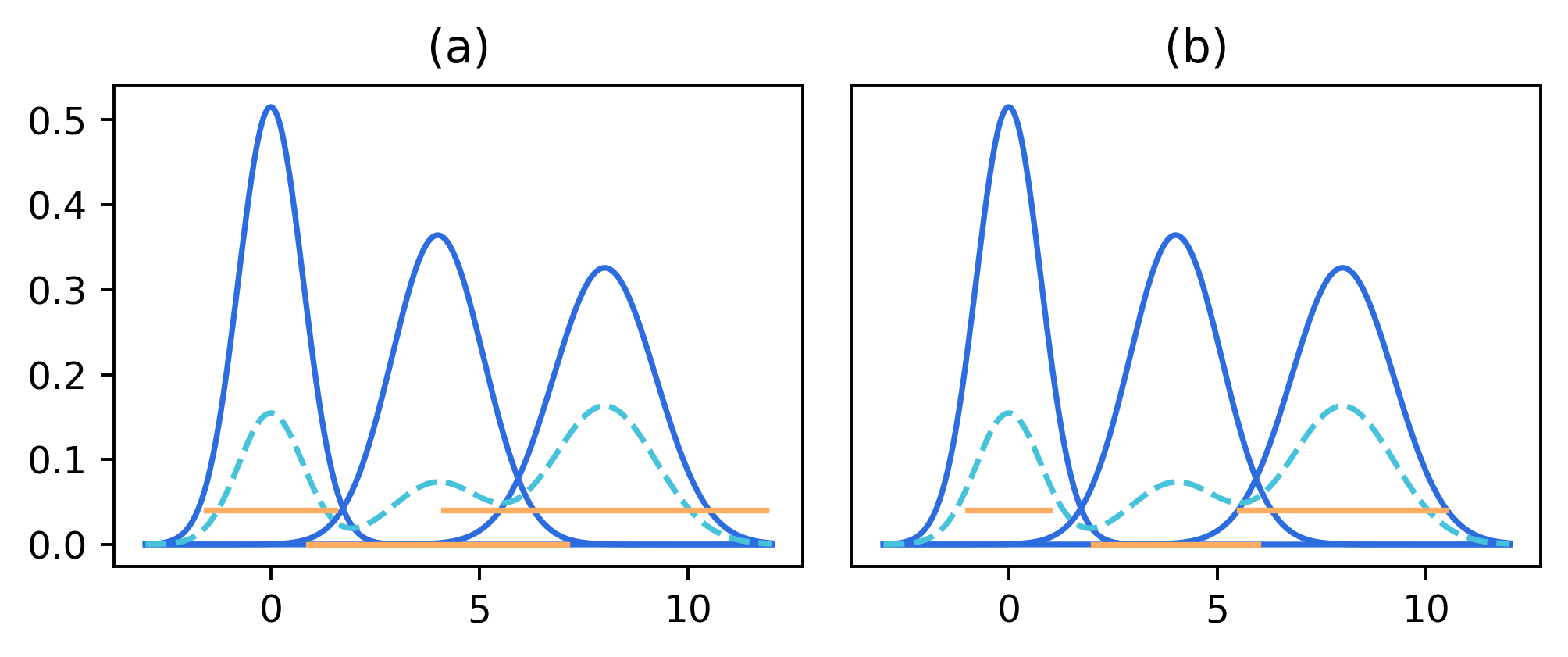
Figure 1: An illustration of intervals produced by D-Mapper. The deep blue line is the probability density function of each component in the GMM. The shallow blue dashed line is the probability density function of the GMM. The orange lines are intervals that produced naturally by symmetry quantile $\alpha$. (a) The quantile $\alpha=0.01$, each interval has pairwise overlap. (b) The quantile $\alpha=0.1$, there is a gap between the first and second interval. The quantile $\alpha$ can control the overlap of intervals, therefore this parameter should be chosen carefully.

In both our simulation and real data experiments, we implement the Gaussian mixture models (GMM) to fit the data due to its simplicity and flexibility. The model inference is done via the expectation maximization (EM) algorithm 2009The . Other mixture models or any distribution with multiple modes can be used as alternatives to the GMM.

By incorporating a mixture model into the Mapper algorithm, it can produce flexible intervals and overlaps. We call this distribution-guided Mapper algorithm as D-Mapper algorithm. With these flexible intervals, we can construct the output graph similar to the classic Mapper algorithm: pulling back these intervals onto the original data space, then applying clustering algorithm within each intervals separately, all sub-groups constitute the vertices of the nerve, and adding an edge between two vertices if there are any shared data points. Algorithm 2 gives details of the D-Mapper.

Algorithm 2 D-Mapper

1:Choose a proper filter function $f$ to project data on the real line,$f:X\rightarrow\mathbb{R}$.

2:Choose a component number $n$ and quantile $\alpha$.

3:Fit projected data to a mixture model.

4:for $i$th component of the mixture model do

5:     Set the $\frac{\alpha}{2}$ quantile $s_{i}$ as the start point of the interval,

6:     Set the $1-\frac{\alpha}{2}$ quantile $e_{i}$ as the end point of the interval,

7:     The interval of $i$th component is $u_{i}=(s_{i},e_{i})$.

8:end for

9:The collection of intervals $\mathcal{U}=(u_{i}),i=1...n,$ is a cover on projected data $f(X)$.

10:Pull back the intervals of projected data, $f^{-1}(\mathcal{U})$.

11:Clustering on the refined cover and build the nerve by clustering result.

The quantile $\alpha$ controls the overlap ratios: larger $\alpha$ leads to lower overlap ratios. Distributions of components in mixture models are often heterogeneous, result in irregular quantile intervals. Proper $\alpha$ selection is crucial to ensure all points are covered.

The Mapper algorithms usually require pairwise overlap (i.e. each interval has overlap with its neighbours)deyTopologicalAnalysisNerves2017 ; dlotkoBallMapperShape2019 ; buiFMapperFuzzyMapper2020 ; chalapathiAdaptiveCoversMapper2021 . For D-Mapper, we also want to preserve the pairwise overlap property (Figure 1 (a)). However, larger $\alpha$ may result in disjoint intervals, Figure 1 (b) gives an example of disjoint intervals caused by improper large $\alpha$. Thus, in this work, we propose a method to find the upper bound of $\alpha$ that guarantees the pairwise overlap property. With this upper bound, we also greatly reduce the range of $\alpha$ to make parameter selection easier. Denote $F_{i}^{-1}$ the inverse of the cumulative density function of the $i$th ordered component, thus the $i$th interval $u_{i}$ is given by $[F_{i}^{-1}(\alpha/2),F_{i}^{-1}(1-\alpha/2)]$, $i=1,\ldots,n$. The idea of this method is to find the upper bound $\alpha^{\prime}$, that guarantee the intersection of each paired neighboring intervals is not empty, $u_{i}\cap u_{i+1}\neq\emptyset$, i.e., $F_{i}^{-1}(1-\alpha/2)\geq F_{i+1}^{-1}(\alpha/2)$, $i=1,2,\ldots,n-1$. Algorithm 3 describes how to find the upper bound of $\alpha$.

Algorithm 3 $\alpha$ upper bound

1:$\boldsymbol{J}$ = $\emptyset$

2:for $i$ in range(0,$n-1$) do

3:     $S_{1}(\alpha)=F_{i}^{-1}(1-\alpha/2)$,

4:     $S_{2}(\alpha)=F_{i+1}^{-1}(\alpha/2)$,

5:     Let $S_{1}(\alpha)=S_{2}(\alpha)$, solve for solution $\alpha_{i}^{\prime}$.

6:     if $\alpha_{i}^{\prime}\geq\alpha^{a}*$ then

7:         $\boldsymbol{J}=\boldsymbol{J}\cup\{i\}$

8:     end if

9:end for

10:$\alpha^{\prime}=min\{\alpha_{i}\}_{i\in\boldsymbol{J}}$.

11:The upper bound of $\alpha$ is $\alpha^{\prime}$, $\alpha\in(0,\alpha^{\prime})$.

Notice that although pairwise overlap is a good property for a Mapper graph, this property is not necessary for all situations. One can construct a good Mapper graph with some paired neighbouring intervals being non-overlap as long as covers can cover all data points. We add one threshold parameter $\alpha^{*}$ to allow for disjoint paired neighbouring intervals (lines 6-10 of Algorithm 3). In practice, we suggest to set $\alpha^{*}=0.005$. As shown in the simulation section, the example of the two disjoint circles does not overlap in pairs (Figure 5 (a) ), since there are no points between the two circles, disjoint paired neighbouring intervals should be presented in the corresponding Mapper output graph.

2.4 Evaluation metric

The silhouette coefficient ($SC$) is often used as a measure to evaluate the quality of (overlap) clustering hanClusterAnalysis2012 . The $SC$ assesses how well the clusters are separated, how close the clusters are, and is stable for overlap clustering. Suppose we have $n$ samples in dataset $D$ that could be divided into $k$ clusters: $C_{1},...,C_{k}$. For a data point $x\in D$, the compactness of the cluster to which $x$ belongs can be defined as:

$$a(x)=\frac{\sum_{x^{\prime}\in C_{i},x\neq x^{\prime}}d(x,x^{\prime})}{|C_{i}|-1},$$

where $d(x,x^{\prime})$ represents the distance between $x$ and $x^{\prime}$, $|C_{i}|$ is the number of data points in cluster $i$. The degree of separation between $x$ and other clusters can be computed as:

$$b(x)=\mathop{\min}_{C_{j}:j\neq i}\bigg{\{}\frac{\sum_{x^{\prime}\in C_{j}}d(x,x^{\prime})}{|C_{j}|}\bigg{\}},$$

And the $SC$ of $x$ is:

$$SC(x)=\frac{b(x)-a(x)}{\max\{a(x),b(x)\}},$$

The value of the $SC$ ranges from $-1$ to $1$. A value close to 1 indicates the point is close to the current cluster, and more distinct from other clusters. If the $SC$ is less than 0, it means the point is closer to other clusters compared to the current cluster, and it usually indicates bad clustering results. The clustering of the whole dataset can be assessed by taking average of the $SC$s of all points.

The $SC$ reflects the clustering quality of data points, but it does not evaluate the topology structure of a Mapper output graph. Figure 2 shows an example of a Mapper graph that has high $SC$ but poor topological structure. The left panel has higher $SC$ but poor topological feature while the right panel has lower $SC$ but good topological structure. Therefore, a metric that evaluates both clustering and topological structure is needed. Although, the topological information encoded in Mapper is well studied theoretically deyTopologicalAnalysisNerves2017 . There is no practical metric to evaluate the topology structure of Mapper graph. Most existing work evaluates the topology structure of Mapper graphs based on the clustering results only. The extended persistence diagram has been proven to be a powerful tool for capturing topological signatures of Mapper graph carriereStructureStabilityOneDimensional2018 . In this manuscripts, we alleviate it to provide a simple quantitative metric for evaluating the topology structure of Mapper output.

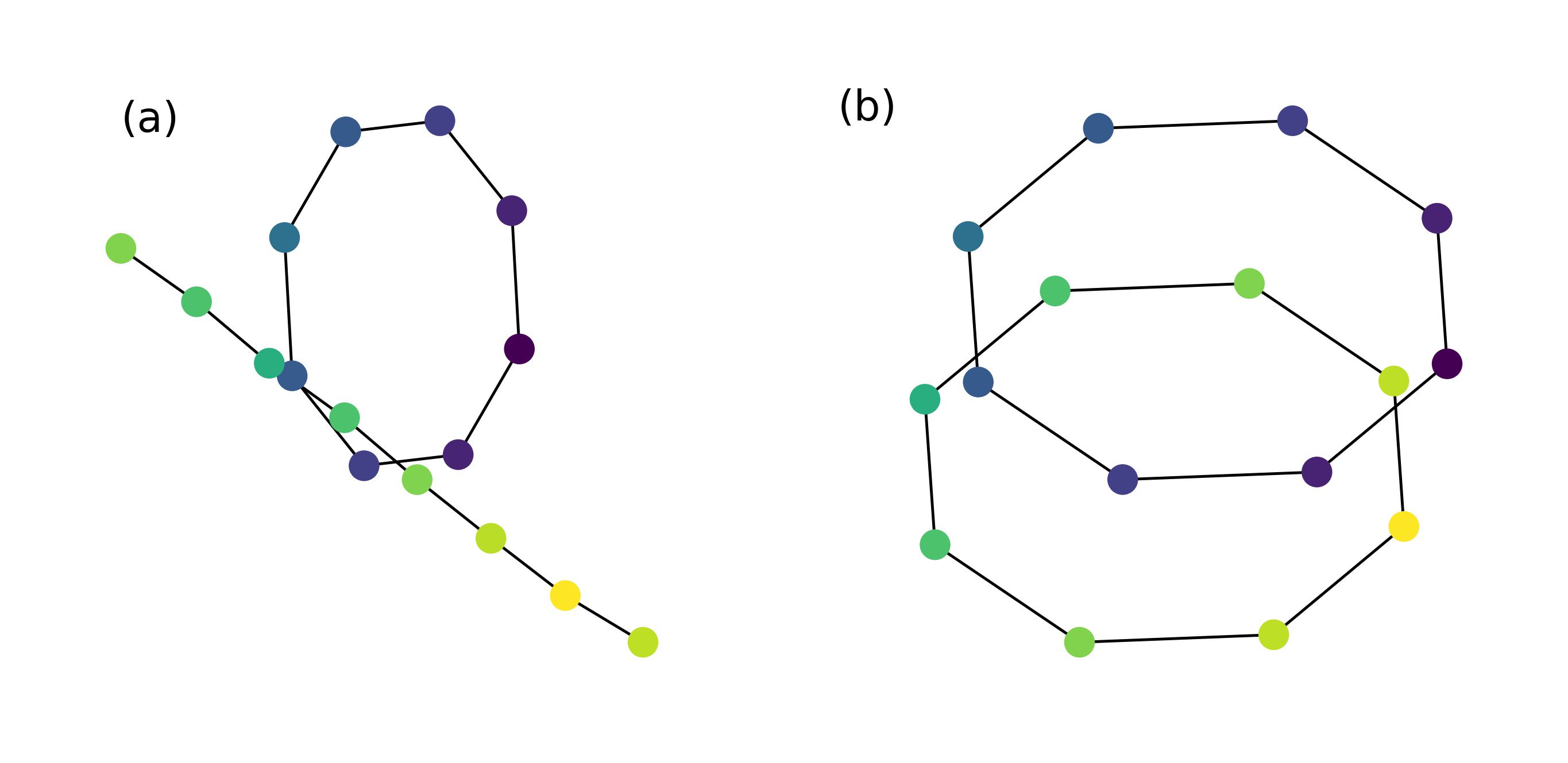
Figure 2: An example of the classical Mapper algorithm has higher $SC$ but poor topological structure, the dataset is shown in Figure 5 (a), the classical Mapper is implemented on this dataset. (a) A graph produced by the classic Mapper with parameters: $n=12,p=0.01$. $SC:0.283$, $SC_{adj}:0.521$. (b) A graph produced by the classic Mapper with parameters: $n=12,p=0.1$, $SC:0.246$, $SC_{adj}:0.812$.

We shall introduce some background of the extended persistence diagram, which are detailed in carriereStructureStabilityOneDimensional2018 . The extended persistence diagram is an extension of the persistence theory. The extended persistence theory uses both sublevel sets and superlevel sets as a filtration to provide more information than the original persistence theory. Like the persistence diagram, the extended persistence diagram spans by points of birth time and death time. As a result, points on the extended persistence diagram can be located anywhere on the plane, unlike the ordinary persistence diagram where points can only be strictly above the diagonal.

Definition 5 (Extended persistence diagram).

The extended persistence diagram is a multiset of points in the Euclidean plane $\mathbb{R}^{2}$. For a graph $G=(V,E)$ and a function defined on its nodes $f:V\rightarrow\mathbb{R}$, the extended persistence diagram is computed by both sublevel sets and superlevel sets, denoted as $Dg(G,f)$. According to the combination of sublevel sets and superlevel sets filtration, each point in the diagram is classified as either $Ord_{0}$, $Rel_{1}$, $Ext^{+}_{0}$ or $Ext^{-}_{1}$.

Briefly speaking, given a graph and a function defined on its nodes, we can compute the extended persistence diagram that reflects the topological features of this graph. For a Mapper graph, the function on a node can be naturally defined as the mean value of points in the node. The points on the diagram can be regarded as signatures of the Mapper graph. However, these signatures are not always meaningful, points near the diagonal are noises. To distinguish noise and real signal, one simple but effective way is to compute the confidence set by bottleneck bootstrap and separate noise and signal based on this confidence set carriereStatisticalAnalysisParameter2017 . Bottleneck bootstrap is an effective way to compute confidence set on a persistence diagram fasyConfidenceSetsPersistence2014 . It uses bootstrap samples to get a bootstrap Mapper graph and then calculate the bottleneck distance from the original Mapper graph. Repeat this step many times, we can obtain an approximate distribution of bottleneck distance. With this distribution we can easily calculate the confidence set.

We introduce a metric to evaluate the quality of the extended persistence diagram dependent on the confidence set, we call this metric the topological signal rate (TSR). The TSR is defined as the number of real signal points divided by the total number of points on the extended persistence diagram, serving as a quantitative indicator of the quality of the extend persistence diagram.

Definition 6 (Topological signal rate).

The topological signal rate is a scalar, it evaluates the quality of a persistence diagram or extended persistence diagram, denoted as TSR:

$$TSR=\frac{N_{signal}}{N},$$

where $N$ is the number of all points on the diagram and $N_{signal}$ is the number of topological signal on the diagram.

An example of an extended persistence diagram and its TSR is illustrated in Figure 3. The gray area is the confidence set estimated by the bottleneck bootstrap. Points inside are noises and those outside are signal points. The TSR in this example is 0.25, indicating poor quality of the corresponding Mapper graph. To get a proper evaluation of the Mapper graph, we can combine the TSR with $SC$ through weighted averaging. We call this metric as adjusted silhouette coefficient.

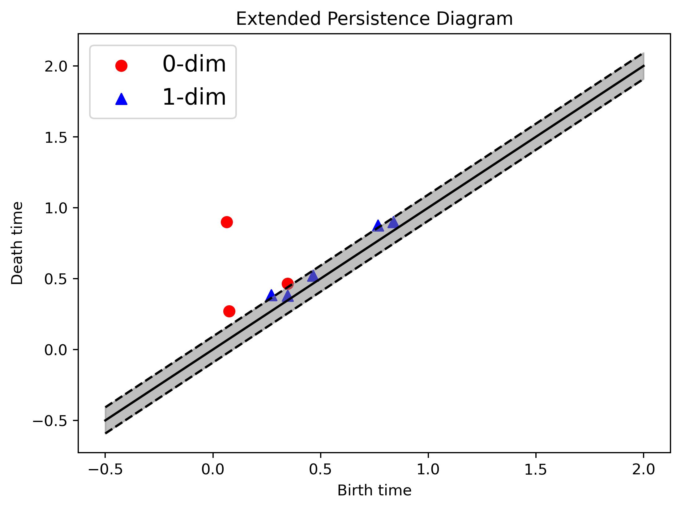
Figure 3: An example of the extended persistence diagram. There are totally 8 points in the diagram, the gray area is computed by the bottleneck bootstrap, points inside this area are noise. Thus, 6 points are noises and 2 points are signals, the TSR is 0.25 .

Definition 7 (Adjusted silhouette coefficient).

The adjusted silhouette coefficient is the weighted average of the normalized $SC$ and the $TSR$, denoted as $SC_{adj}$, this value can serve as a metric to evaluate Mapper type algorithms:

$$SC_{adj}=w_{1}SC_{norm}+w_{2}TSR,$$

where TSR is given by Definition 6, representing the topological signal rate, $SC_{norm}=\frac{SC+1}{2}$ is the normalized value of $SC$, and we choose $w_{1}=w_{2}=0.5$ here to give same weights of clustering and topological structure.

Figure 2 compares the value of $SC_{adj}$ with the original $SC$. The original $SC$ overlooks the topological structure of Mapper graph, while the $SC_{adj}$ can give a reasonable evaluation. In the next section, we show more examples of $SC_{adj}$ and validate its effectiveness through some comparisons.

3 Simulation

In this section, we compare our proposed D-Mapper algorithm with the classic Mapper algorithm via several experiments. In this paper, we implement D-Mapper by expanding the Mapper algorithm in the KeplerMapper package version 2.0.1 KeplerMapper_JOSS in python version 3.11.0. The extended persistence diagram and bottleneck bootstrap are computed by a python package GUDHI version 3.8.0 gudhi:urm .

We compare our proposed D-Mapper algorithm with the classic Mapper algorithm using the metric $SC_{adj}$ and $SC_{norm}$. We set the interval number $n$ to be identical for both algorithms and use the same clustering algorithm within each hypercube. The clustering method is the density-based spatial clustering of applications with noise (DBSCAN) implemented in the scikit-learn library version 1.1.3. We use a fixed grid to find the best model concerning the $SC_{adj}$ for both the D-Mapper and the classic Mapper. $50$ equally spaced grids in range $(0,\alpha_{max})$ are used to select parameter $\alpha$ in the D-Mapper. Similarly, $50$ equally spaced grids in range $(0,0.5)$ are used to tune the overlap percentage $p$ in classic Mapper algorithm. The bottleneck bootstrap sampling steps are set to $100$ to compute $85$ percent confidence regions. In the next section, we compare the D-Mapper with the classic Mapper on several examples.

3.1 Two disjoint circles

This dataset is created by sampling points randomly from two disjoint circles with centers $(0,0)$ and $(3,0)$ and a radius of $1$. $5000$ points are uniformly sampled on each circle. Figure 5 (a) provides a visualization of the sampled data points. This dataset has a distinctive shape and provides a straightforward performance comparison between the classical Mapper and D-Mapper algorithms.

In this experiment, we choose the filter function to be a function that projects the original data onto the X-axis. We set the number of intervals $n$ to $12$. The parameters $p$ of the classic Mapper algorithm and parameter $\alpha$ of the D-Mapper are tuned via grid search, $n=12,p=0.02$, $n=12,\alpha=0.127$. The comparison of different evaluation metrics is shown in Table 1 and Figure 4. In Figure 4, the color of a node indicates the average value of projected data in the node. The output graphs of the classic Mapper and D-Mapper are similar, and both algorithms capture the topological features of the dataset effectively without noise, result in a TSR of 1 for both algorithms. The D-Mapper performs better than the classic Mapper in terms of clustering, as evidenced by its higher $SC_{norm}$. This indicates that D-Mapper has an advantage in identifying more meaningful clusters. Moreover, we show cases that both Mapper algorithms concerned on $SC$ only in Figure 4 (c) and (d). In these two cases the $SC_{norm}$ are higher but the TSR are lower than the results concerned on $SC_{adj}$. The topology structures of these two cases are obviously different from the dataset in these two figures. The distinct results in this example validate the utility of our proposed metric. It provides a quantitative approach for evaluating Mapper-type algorithms from both topological signal preservation and clustering.

Table 1: Results of the D-Mapper and classic Mapper on two disjoint circles dataset.The $1$st and $3$rd rows are results that with the larger $SC_{adj}$. The $2$nd and $4$th rows are cases when the output graphs have larger $SC$ values, but lower TSRs.

Algorithm	$SC_{norm}$	TSR	$SC_{adj}$
Classic Mapper	0.640	1.00	0.820
Classic Mapper	0.642	0.40	0.521
D-Mapper	0.716	1.00	0.858
D-Mapper	0.733	0.33	0.533

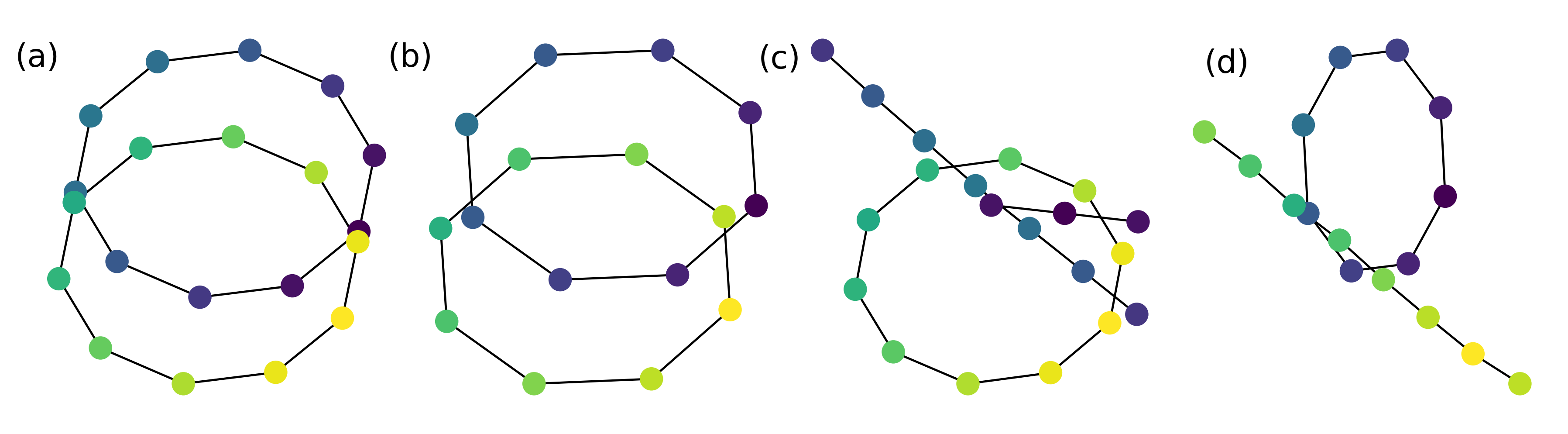
Figure 4: Results of the classic Mapper and D-Mapper on the two disjoint circles. (a) The output graph of the classic Mapper with the largest $SC_{adj}$ (the $1$st row of Table 1): $n=12,p=0.02$. (b) The output graph of D-Mapper with the largest $SC_{adj}$ (the $3$rd row of Table 1): $n=12,\alpha=0.127$. (c) An example produced by the D-Mapper with larger $SC$ but lower TSR (the $2$nd row of Table 1): $n=12,\alpha=0.159$. (d) An example produced by the classic Mapper with larger $SC$ but lower TSR (the $4$th row of Table 1): $n=12,p=0.005$.

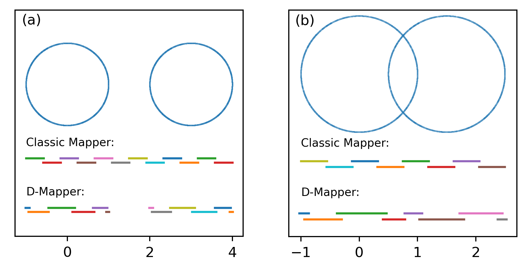
Figure 5: (a) Upper panel: visualization of two disjointed unit circles whose centers are (0,0) and (3,0) respectively. Bottom panel: the intervals produced by both Mappers. The intervals produced by D-Mapper have a gap between two circles, these intervals are more reasonable than classic Mapper’s. Because there are no points between two disjointed circles, the intervals between two circles are meaningless. (b) Upper panel: a visualization of two intersecting unit circles dataset whose centers are $(0,0)$ and $(1.5,0)$ respectively. Bottom panel: the intervals produced by both Mappers. The intervals of D-Mapper can assign more reasonable intervals than classic Mapper on the intersecting part.

3.2 Two intersecting circles

In this section, we compare the performance of the D-Mapper and the classic Mapper on a two intersecting circles dataset shown in Figure 5 (b). The data points are generated from two intersecting circles with a radius of 1 and centers (0,0) and (1.5,0), respectively. The data generating process is similar to the previous example, 5000 points are sampled from each circle. The filter function is the same as in the previous example. For the classic Mapper algorithm, the number of intervals $n$ is set to $8$ and the overlap rate $p$ is chosen as $0.02$. As for the D-Mapper algorithm, the number of intervals is the same as the classic Mapper’s and the parameter $\alpha$ is tuned to $0.088$. The result of this experiment is given in Figure 6 and Table 2. The D-Mapper outperforms the classic Mapper concerned on $SC$ scores, and has the same topological signal rate as the classic Mapper. As a result, the $SC_{adj}$ of D-Mapper is higher than the classic Mapper. Similar with the two disjoint circles example, Figure 6 (c) and (d) also show cases that when the metric $SC$ fails.

Table 2: Results of the D-Mapper and classic Mapper on two disjoint circles dataset. The $1$st and $3$rd rows are results that with the larger $SC_{adj}$. The $2$nd and $4$th rows are cases when the output graphs have larger $SC$ values, but lower TSRs.

Algorithm	$SC_{norm}$	TSR	$SC_{adj}$
Classic Mapper	0.574	1.00	0.787
Classic Mapper	0.577	0.25	0.414
D-Mapper	0.640	1.00	0.820
D-Mapper	0.662	0.50	0.581

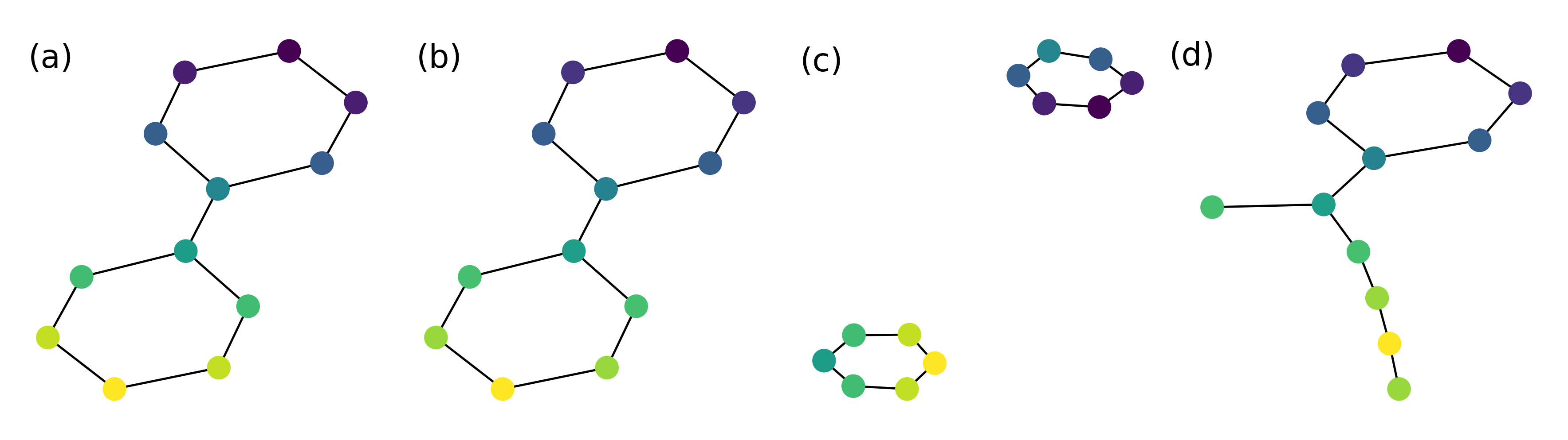
Figure 6: Results of the classic Mapper and D-Mapper on the two intersecting circles. (a) The output graph of the classic Mapper with the largest $SC_{adj}$ (the $1$st row of Table 2): $n=8,p=0.02$. (b) The output graph of D-Mapper with with the largest $SC_{adj}$ (the $3$rd row of Table 2): $n=8,\alpha=0.088$. (c) An example produced by the D-Mapper with larger $SC$ but lower TSR (the $2$nd row of Table 2): $n=8,\alpha=0.12$. (d) An example produced by the classic Mapper with larger $SC$ but lower TSR (the $2$nd row of Table 2): $n=8,p=0.02$.

Both the results of the two disjoint circles and the two intersecting circles indicate that our proposed metric $SC_{adj}$ is more stable than the metric $SC$ measuring both the quality of overlap clustering and extended persistence homology of output of Mapper type algorithm.

3.3 3D cat dataset

In this experiment, we compare the D-Mapper algorithm with the classic Mapper algorithm on a 3D cat dataset with a more complex topology structure. The 3D cat dataset is originally created by 2004Deformation . Figure 7 (a) shows a visualization of the 3D cat dataset. The filter function returns the averaged pairwise distance between the points and all other points. The parameters of the classic Mapper are set to $n=9,p=0.32$; and the parameters of the D-Mapper are set to $n=9,\alpha=0.01$. The clustering method is DBSCAN with a radius of $0.1$ and a minimum of samples $5$. The results and evaluation metrics are shown in Figure 7 and Table 3. The D-Mapper algorithm results higher $SC_{norm}$ scores and the same TSR compares to the classic Mapper algorithm. The output graph of the D-Mapper has one more loop than the classic Mapper, which represents the ears of cats (yellow dots in Figure 7 c-d). This example also shows that the D-Mapper could capture subtle features of complex objects better than the classic Mapper.

Table 3: Results of the classic Mapper and D-Mapper on the 3D cat dataset.

Algorithm	$SC_{norm}$	TSR	$SC_{adj}$
Classic Mapper	0.480	1.0	0.740
D-Mapper	0.510	1.0	0.755

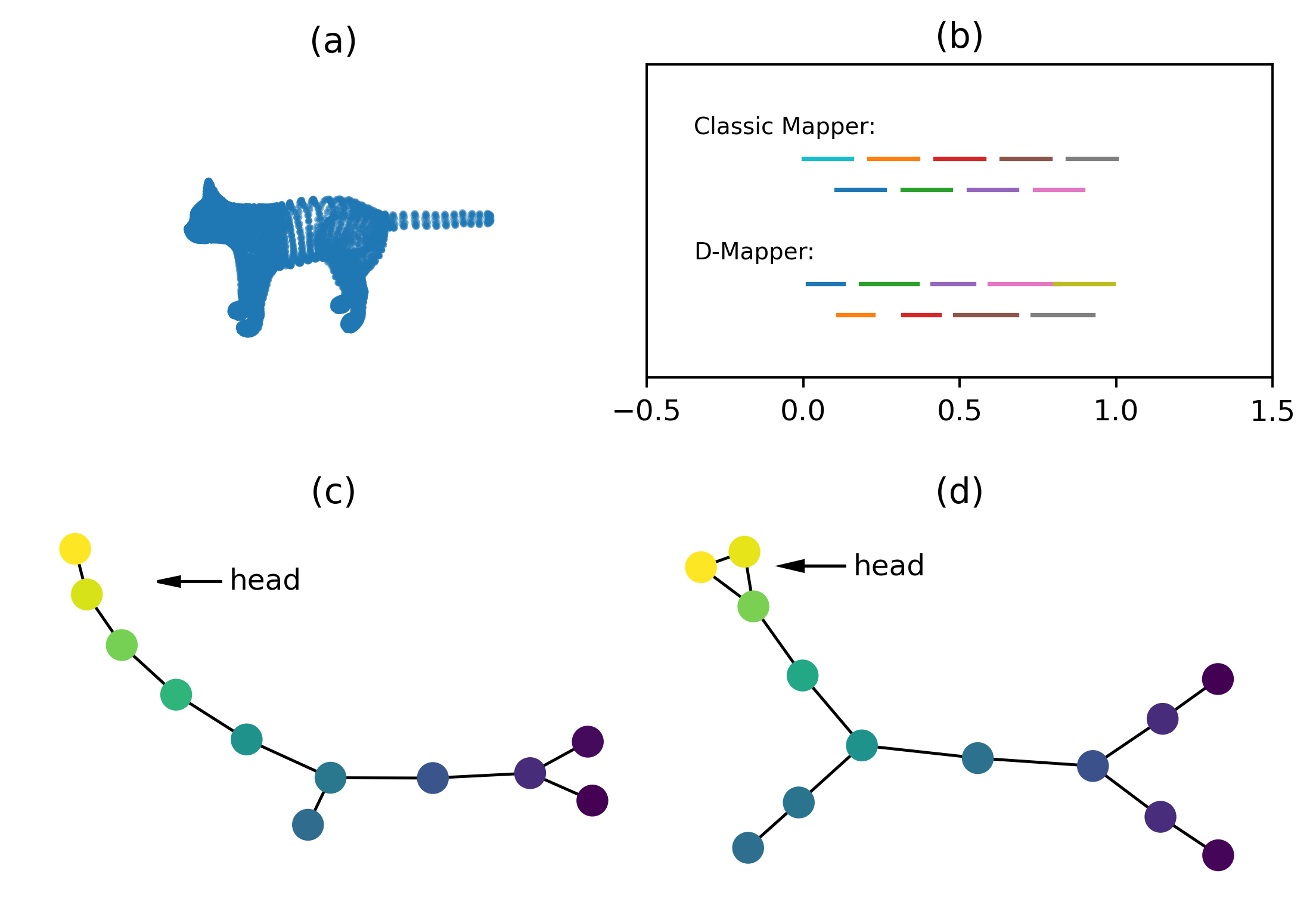
Figure 7: Results of the classic Mapper and D-Mapper on the 3D cat dataset. (a) Visualization of the 3D cat dataset. (b) The intervals produced by both Mappers. The intervals of both Mappers are very close except intervals near to 1, this difference gives more details on cat head in D-Mapper. (c) The graph of the classic Mapper with the largest $SC_{adj}(0.740)$: $n=9,n=0.32$. (d) The graph of D-Mapper with the largest $SC_{adj}(0.755)$: $n=9,\alpha=0.01$.

3.4 Summary of experiments

In all experiments, the D-Mapper outperforms the classic Mapper algorithm concerning on the metric $SC_{adj}$. The $SC_{norm}$ of the D-Mapper are all higher than the classic Mapper algorithm, and all TSRs are $1$. This indicates that the D-Mapper can achieve better clustering than the classic Mapper algorithm while outputing high quality reeb graph approximations. Note that we tune parameters by grid search the highest $SC_{adj}$, thus the TSR is relatively high. In many cases the TSR could be low, as we show in Table 1 and Table 2. Our experimental results also indicate that our proposed metric $SC_{adj}$ is more stable than the metric $SC$.

4 Application

In this section, we apply our proposed method to a real dataset. The Covid-19 pandemic poses an enormous threat to global health and economic. To combat the epidemic, one of the fundamental tasks is identifying and monitoring the mutation of the SARS-COV-2 coronavirus. Studying virus evolution helps understand the basic biological characteristics, develop vaccines and drugs, and forecast trends. A traditional way to study viral mutations is constructing phylogenetic trees based on genetic sequences. However, tree structure representations can only show vertical processes. Whereas, some processes are horizontal. For virus, the homologous recombination and reassortment are typical examples lead to non-tree-like representation chanTopologyViralEvolution2013 . We apply the D-Mapper algorithm on a SARS-COV-2 coronavirus RNA sequences dataset, serving as an alternative tool to investigate both the vertical and horizontal processes of viral mutations. The dataset contains $357$ SARS-COV-2 coronavirus RNA sequences in China with different lineages from GenBase (https://ngdc.cncb.ac.cn/genbase/) in National Genomics Data Center cncb-genbase2023 .

We first compute the distance matrix of input sequences, several methods are available to compute distance between RNA or DNA sequences, such as alignment algorithm based or likelihood based method, however these methods are computational expensive for large whole DNA or RNA sequences dataset. To simplify computation, we use $k$-mers frequency vector as a representation of every sequence and compute pairwised distance base on these vectors. We choose $k=3$, then every sequence is a $64$ dimension vector. Since these RNA sequences have high similarities, we perform a min-max scaling on them. Finally, we calculate the mean of each row as the filtered data.

The number of intervals are set to $n=15,\alpha=0.01$ via grid tunning. The DBSCAN with a radius of $0.6$ and a minimum of samples $3$ is chosen in the clustering algorithm. The results are shown in Figure 8. The output structure represents the evolution process of these lineages. The loop structure represents the horizontal evolution process. The lineages of the two isolated nodes may indicate significant differences from others, these lineages may warrant further investigation.

Some important lineages in these nodes are shown in Table 4. The bottom green loop nodes contain many XBB variants, which from the recombination of two subvariants and cause large-scale infections worldwide VirologicalCharacteristicsSARSCoV22023 . The recombination of virus is a typically horizontal evolution process and the D-Mapper algorithm can provide some insights of these rapid and complex evolution process.

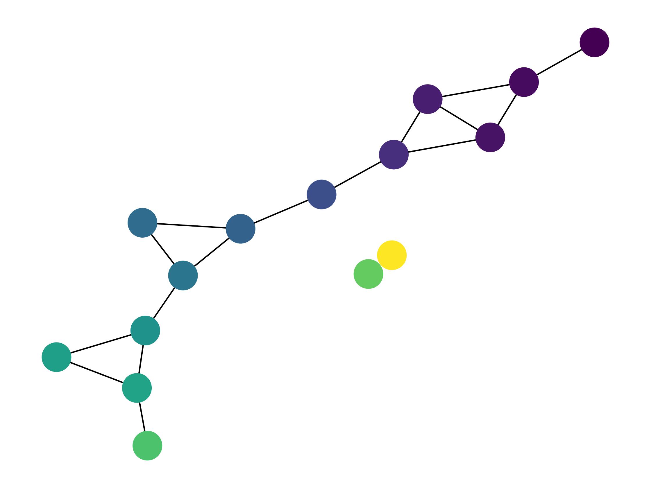
Figure 8: The result of D-Mapper on SARS-COV-2 dataset.

5 Conclusion

In this paper, we propose a distribution-guided Mapper algorithm (D-Mapper) to relax the fixed intervals (or fixed overlap ratios) restriction in the classic Mapper algorithm. Our proposed algorithm combines a mixture model and the Mapper algorithm to obtain irregular intervals based on the density of projected data. With these irregular intervals, the D-Mapper algorithm can gain deeper topological insights and enhance clustering outcome. To validate the effectiveness of our proposed algorithm, we introduce the $SC_{adj}$ score to combine $SC$ scores and extended persistence diagram as a metric to reflect the performance of overlap clustering and persistence homology. We also conduct numerical experiments with different complexity to evaluate the D-Mapper algorithm by the $SC_{adj}$. The D-Mapper outperforms the classical Mapper algorithm under various parameter settings in all experiments. We also apply the D-Mapper algorithm to the SARS-COV-2 coronavirus RNA sequences, and the result shows that the D-Mapper algorithm can reflect both the vertical and horizontal evolution processes.

Our proposed algorithm is a probabilistic model-based approach that uses data intrinsic characteristics and probability models to generate distribution-guided covers and improved topological features. It is a viable alternative to non-probabilistic approaches. With the D-Mapper, once we get the distribution of the projected data, and we further can get the intervals from each distribution by quantile. Theoretically, the distribution of original data can be computed by transformation of distributions if the filter function is well proposed, this may be helpful for further theoretical analysis.

The selection of optimal number of components remains a difficult problem to address. One possible solution is to use non-parametric mixture model, such as the Dirichlet process, by introducing the Dirichlet process prior to adaptively choose the number of components. Another approach is to apply the information criteria like AIC or BIC to find a proper number of components for the mixture model.

Table 4: Lineages in some important nodes. Only some important shared lineages in loop nodes are shown in this table, the complete information can be found in the supplementary materials.

Nodes	Lineages
Yellow isolated node	XBB.1.5.28, BN.1.1, EJ.2
Green isolated node	FL.15, EP.1, FL.2.2.1, FY.3.3, XBF.7, BQ.1.2
Bottom green loop nodes	BA.5.1.3, XBB.1.9.2, XBB.1.42, XBB.1.16.7, XBB.1.17.1
Middle blue loop nodes	BA.2.86, FY.1.1, XBB.1.12, XBB.1.5.32, FL.2.3.1, FL.10.1
Upper purple loop nodes	EG.4.2, EG.5.2, FY.2, FL.1, XBB.2.3.8

6 Competing interests

No competing interest is declared.

7 Acknowledgments

This project was supported by the Shanghai Science and Technology Program (No. 21010502500), the startup fund of ShanghaiTech University.

References

- [1] Khaled Almgren, Minkyu Kim, and Jeongkyu Lee. Mining Social Media Data Using Topological Data Analysis. In 2017 IEEE International Conference on Information Reuse and Integration (IRI), pages 144–153, 2017.
- [2] Quang-Thinh Bui, Bay Vo, Hoang-Anh Nguyen Do, Nguyen Quoc Viet Hung, and Vaclav Snasel. F-Mapper: A Fuzzy Mapper clustering algorithm. Knowledge-Based Systems, 189:105107, 2020.
- [3] Gunnar Carlsson. Topology and data. Bulletin of the American Mathematical Society, 46(2):255–308, 2009.
- [4] Mathieu Carrière, Bertrand Michel, and Steve Oudot. Statistical analysis and parameter selection for mapper. Journal of Machine Learning Research, 19(12):1–39, 2018.
- [5] Mathieu Carrière and Steve Oudot. Structure and Stability of the One-Dimensional Mapper. Foundations of Computational Mathematics, 18(6):1333–1396, 2018.
- [6] Nithin Chalapathi, Youjia Zhou, and Bei Wang. Adaptive Covers for Mapper Graphs Using Information Criteria. In 2021 IEEE International Conference on Big Data (Big Data), pages 3789–3800, Orlando, FL, USA, December 2021. IEEE.
- [7] Joseph Minhow Chan, Gunnar Carlsson, and Raul Rabadan. Topology of viral evolution. Proceedings of the National Academy of Sciences, 110(46):18566–18571, 2013.
- [8] Frédéric Chazal and Bertrand Michel. An introduction to Topological Data Analysis: Fundamental and practical aspects for data scientists. Frontiers in Artificial Intelligence, 4, 2021.
- [9] CNCB-NGDC Members and Partners. Database Resources of the National Genomics Data Center, China National Center for Bioinformation in 2023. Nucleic Acids Res, 51(D1):D18–D28, 2023.
- [10] Ramin Dehghanpoor, Fatemeh Afrasiabi, and Nurit Haspel. Using Topological Data Analysis and RRT to Investigate Protein Conformational Spaces. page 10.
- [11] Tamal K. Dey, Facundo Mémoli, and Yusu Wang. Topological Analysis of Nerves, Reeb Spaces, Mappers, and Multiscale Mappers. In 33rd International Symposium on Computational Geometry (SoCG 2017), volume 77 of Leibniz International Proceedings in Informatics (LIPIcs), pages 36:1–36:16, 2017.
- [12] Paweł Dłotko. Ball mapper: a shape summary for topological data analysis, January 2019.
- [13] Brittany Terese Fasy, Fabrizio Lecci, Alessandro Rinaldo, Larry Wasserman, Sivaraman Balakrishnan, and Aarti Singh. Confidence sets for persistence diagrams. The Annals of Statistics, 42(6):2301–2339, 2014.
- [14] Jiawei Han, Micheline Kamber, and Jian Pei. Cluster Analysis. In Data Mining, pages 443–495. Elsevier, 2012.
- [15] Trevor Hastie, Robert Tibshirani, Jerome H. Friedman, and James Franklin. The elements of statistical learning: Data mining, inference and prediction. by. The Mathematical Intelligencer, 27(2):83–85, 2009.
- [16] Satanik Mitra and Kameshwar Rao JV. Experiments on Fraud Detection use case with QML and TDA Mapper. In 2021 IEEE International Conference on Quantum Computing and Engineering (QCE), pages 471–472, 2021.
- [17] Monica Nicolau, Arnold J. Levine, and Gunnar Carlsson. Topology based data analysis identifies a subgroup of breast cancers with a unique mutational profile and excellent survival. Proceedings of the National Academy of Sciences, 108(17):7265–7270, 2011.
- [18] The GUDHI Project. GUDHI User and Reference Manual. GUDHI Editorial Board, 3.8.0 edition, 2023.
- [19] Abbas H Rizvi, Pablo G Camara, Elena K Kandror, Thomas J Roberts, Ira Schieren, Tom Maniatis, and Raul Rabadan. Single-cell topological RNA-seq analysis reveals insights into cellular differentiation and development. Nat Biotechnol, 35(6):551–560, 2017.
- [20] Gurjeet Singh, Facundo Mémoli, and Gunnar Carlsson. Topological Methods for the Analysis of High Dimensional Data Sets and 3D Object Recognition. In Symposium on Point Based Graphics, pages 91–100.
- [21] Yara Skaf and Reinhard Laubenbacher. Topological data analysis in biomedicine: A review. Journal of Biomedical Informatics, 130:104082, 2022.
- [22] Rw Sumner and J Popovic. Deformation transfer for triangle meshes. Acm Transactions on Graphics, 23(3):399–405, 2004.
- [23] Ito J. Uriu K. et al. Tamura, T. Virological characteristics of the SARS-CoV-2 XBB variant derived from recombination of two Omicron subvariants. Nat Commun, 14(1):2800, 2023.
- [24] Arisa Toda, Satoru Hiwa, Kensuke Tanioka, and Tomoyuki Hiroyasu. Visualization, Clustering, and Graph Generation of Optimization Search Trajectories for Evolutionary Computation Through Topological Data Analysis: Application of the Mapper. In 2022 IEEE Congress on Evolutionary Computation (CEC), pages 1–8, 2022.
- [25] Hendrik Jacob van Veen, Nathaniel Saul, David Eargle, and Sam W. Mangham. Kepler mapper: A flexible python implementation of the mapper algorithm. Journal of Open Source Software, 4(42):1315, 2019.