High order multiscale methods for advection–diffusion
equation with highly oscillatory boundary condition

Abstract

In this paper we propose high order numerical methods to solve a 2D advection–diffusion equation, in the highly oscillatory regime. We use an integrator strategy that allows the construction of arbitrary high–order schemes which leads to an accurate approximation of the solution without any time step–size restriction. This paper focuses on the time multiscale challenge of the problem, that comes from the velocity, an $\varepsilon-$periodic function, whose expression is explicitly known. $\varepsilon$–uniform third order in time numerical approximations are obtained. For the space discretization, this strategy is combined with high order finite difference schemes. Numerical experiments show that the proposed methods achieve the expected order of accuracy.

1 Introduction

In this paper, we develop numerical schemes to solve a model of the diffusion of particles within a fluid in the presence of an oscillating flow, caused by the oscillation of a certain body or trap. This topic has practical applications, particularly in understanding the relationship between living cell membranes (acting like traps) and diffusing particles (for example vital substances). In such an application, an important factor would be the rate at which these substances are captured by the trap. To investigate the capture rate, a biomimetic model has been created [1, 2, 3], where an oscillating air bubble emulates a fluctuating cell, and the flow of charged surfactants represents the diffusing substances (see Fig. 1 (a)). In this specific model, the surfactants consist of anions and cations with different configurations: the cations are hydrophilic, while the anions have a hydrophilic head and a hydrophobic tail, leading to their absorption at the air–water interface. The shape oscillations of drops in another fluid with surfactant has been largely investigated, because of the multiple applications in nuclear physics, meteorology and chemical engineering [4, 5, 6]. In [7], the authors study the parameters that influence the oscillation frequency of an interface, with and without surfactants.

\begin{overpic}[abs,width=346.89731pt,unit=1mm,scale={.25}]{Figures/schematic_setup} \put(-4.0,47.0){(a)} \end{overpic}

\begin{overpic}[abs,width=368.57964pt,unit=1mm,scale={.25}]{Figures/V_x_delta_05.pdf} \put(27.5,45.0){{$\delta$}} \put(9.0,47.0){{$\Omega^{\delta}_{\rm b}$}} \put(45.0,47.0){{$\Omega_{\rm f}$}} \put(-1.0,47.0){(b)} \end{overpic}

Figure 1: (a): Scheme of the experimental setup. On the right there is a zoom in of the anions behaviour at the air–surface of the bubble, with the hydrophobic tails inside the air bubble, and the hydrophilic heads on the surface. (b) Scheme of the potential $V(x)$, defined in Eq. (2), where $\delta$ is the thickness of the attractive-repulsive part.

When studying the diffusion of particles in a moving fluid, it is fundamental to refer to advection–diffusion equations, that are important in many branches of engineering and applied sciences [8, 9, 10, 11]. In this type of equations, two main terms appear: a non–dissipative, advective, hyperbolic term and a dissipative, diffusive, parabolic one. Numerical methods generally perform well when diffusion dominates the equation. On the contrary, when advection prevails, undesirable phenomena, such as spurious oscillations or excessive numerical diffusion, may happen, and some stability property needs to be satisfied [12]. One possible approach to solve this issue is the implementation of fine mesh refinement, e.g., satisfying a suitable stability condition on the mesh Péclet number [13] (if we consider central differences instead of an upwind discretization), although it may not always be practical due to the significant increase of computational cost. Other approaches have been proposed, e.g. in [14], where a relaxation method, based on finite differences schemes, was developed for one–dimensional advection–diffusion equation, in the steady state regime, and in the presence of constant coefficients.

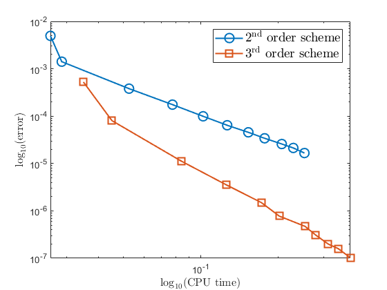
Figure 12: Comparison of the CPU time between the $2^{\rm nd}$ order scheme (blue circles, see Eqs. (44–45)) and the $3^{\rm rd}$ order scheme (red squares, see Eqs. (46–47)). We show the error defined in Eq. (65) with $\Delta t_{\rm ref}=10^{-5}$ for different $\Delta t\in\{1/5,1/10,1/20,1/30,1/40,1/50,1/60,1/70,1/80,1/90,1/100\}$. The parameters of the test are: $\varepsilon=10^{-3},N=20,A=100,\delta=10^{-3},t_{\rm fin}=1$ and $D=0.01$.

The main focus of this paper is the development of a high–order accurate methods in space and time accurate numerical method to solve advection–diffusion equations with highly oscillatory boundary. Low order numerical schemes are more commonly used because of their simpler implementation. However, when considering efficiency, even if high–order methods require greater programming efforts and more computational operations per grid point, they can significantly reduce the number of grid points needed to achieve a given error tolerance (see, e.g., Fig. 12). In multi–dimensional scenarios, this reduction can lead to substantial decrease of computational time and memory requirements, potentially by orders of magnitude.

There are different classes of high order methods for solving time–dependent convection–dominated PDEs, from the high order weighted essentially non–oscillatory (WENO) schemes, capable of maintaining the robustness that is common to Godunov–type methods [15, 16], to the implicit–explicit (IMEX) Runge Kutta methods suitable for time dependent partial differential systems which contain stiff and non stiff terms [17, 18, 19, 20]. Here, we are interested in solving an advection–diffusion equation, in the highly oscillatory regime. This work is part of a long time project, where the fluid velocity is a $\varepsilon$–periodic function (with $\varepsilon\ll 1$), that we suppose explicitly known. Numerous examples of oscillatory flows, both in terms of modeling and numerical treatment, can be encountered in the existing literature ([8, 21, 22, 23]).

When different time scales appear in the same equation, standard numerical methods produce errors of the order $\Delta t^{p}/\varepsilon^{q}$ (where $\Delta t$ is the time step), for some positive $p$ and $q$. In this way, to obtain the desired accuracy, there is a restriction on the time step, i.e., $\Delta t\ll\varepsilon^{q/p}$, that becomes prohibitive for small values of $\varepsilon$. We will follow the strategy adopted in [24, 25, 26, 27, 28] although in the different contexts of Vlasov–Poisson equations, Klein–Gordon and nonlinear Schrödinger equations, to obtain a robust scheme that is able to deal with a large range of $\varepsilon\in(0,1]$ (being small or not), since our goal is to obtain a numerical scheme that is uniformly accurate in $\varepsilon$. We start from a first order scheme, as we did in [29], and proceed to derive second and third order methods through recursive steps.

The problem of surfactants diffusion, that are adsorbed at the surface of a moving cell, has been investigated by several authors [3, 30, 31, 32, 33, 34, 35, 36] and the starting model for the evolution of single species carriers is the one described in [30], where the authors introduced the local concentration of ions $c=c(\vec{x},t)$, whose time evolution in a static fluid is governed by the conservation law

$$\frac{\partial c}{\partial t}=-\nabla\cdot J.$$ (1)

For simplicity, here we describe only the one space dimension model (see [29, 30] for more details and dimensions). We assume that the fluid domain, which is not affected by the bubble, is $\Omega^{\delta}_{\rm f}=[L\delta,1]$, and that the attractive-repulsive mechanism of the bubble is simulated inside a thin region $\Omega^{\delta}_{\rm b}=[-\delta,L\delta]$, with $L$ a constant of order 1. It means that the potential $V(x)=0$ for $x\in\Omega^{\delta}_{\rm f}$.

Particles near a bubble are initially attracted by its surface. However, when a particle gets extremely close to the surface, it experiences a repulsive force, due to the impermeability of the air bubble. To simulate this behaviour, in [30] we choose the Lennard–Jones potential (LJ) as a prototypical attractive–repulsive potential, as follows

$$V(x)=E\left(\left(\frac{x+\delta}{\delta}\right)^{-12}-2\left(\frac{x+\delta}{\delta}\right)^{-6}\right),$$ (2)

where $\delta$ denotes the range of the potential and $E$ represents the depth of the well, (see Fig. 1 (b)).

In [30] we proposed a multiscale model, based on asymptotic expansion in $\delta$, to describe this adsorption–desorption behaviour. The space multiscale nature derives from the potential that is not negligible only in $\Omega^{\delta}_{\rm b}$, which is very small compared to the entire domain. Summarizing, the 1D multiscale model for a single carrier, in the low concentration approximation, can be obtained for $\delta\ll 1$ (in general, for $\delta/L_{x}\ll 1$ where $L_{x}$ is the length of the 1D domain) as follows:

$$\frac{\partial c}{\partial t} =D\frac{\partial^{2}c}{\partial x^{2}}\quad{\rm{in}}\,x\in[0,1]$$ (3)

$$\frac{\partial c}{\partial x} =0\quad{\rm{at}}\,x=1,\qquad\mathcal{M}\frac{\partial c}{\partial t}=D\frac{\partial c}{\partial x}\quad{\rm{at}}\,x=0$$ (4)

and

$$\mathcal{M}=\delta\int_{0}^{L+1}\exp\left(-U(\zeta)\right)d\zeta.$$ (5)

where $U(\zeta)=\phi\left(\zeta^{-12}-2\zeta^{-6}\right)$ is a non dimensional form of the potential $V(x)$, with $\zeta=1+x/\delta\in[0,L+1]$ is a rescaled variable, $L$ is the distance at which the potential $U$ is negligible and $\displaystyle\phi={E}/{k_{B}T}$. In our case, we pose $L=2$.

When considering the flow velocity, the role of oscillating traps becomes crucial to calculate their rates of adsorption and desorption at their surface. In our work [37], we introduce an advection term into the diffusion equation to account for fluid movement caused by the oscillations of the bubble.

In the presence of a moving fluid, the conservation law for the local concentration of ions $c=c(\vec{x},t)$ is the same as (1)

$$\frac{\partial c}{\partial t}=-\nabla\cdot\vec{J},\quad{\rm in}\,\mathcal{S},$$ (6)

where $\mathcal{S}\subset\mathbb{R}^{2}$. However, this time the flux term $\vec{J}$ contains a diffusion and an advection term,

$$\vec{J}=\ -D\nabla c-c\,\vec{u},\quad t\in[0,t_{\rm fin}]$$ (7)

where $t_{\rm fin}>0$, $D$ is the diffusion coefficient, $\vec{u}=\vec{u}(\vec{x},t/\varepsilon)\in\mathbb{R}^{2}$ is the velocity and it is explicitly known, and it is assumed to be a periodic vector function of time with period equal to $\varepsilon\in]0,\varepsilon_{0}]$, for some $\varepsilon_{0}>0$. We add a subscript $\varepsilon$ on the concentration $c_{\varepsilon}=c$, to emphasize its dependence on the oscillation period, and at the end, the system reads

$$\frac{\partial c_{\varepsilon}}{\partial t}=D\Delta c_{\varepsilon}+\nabla\cdot(c_{\varepsilon}\vec{u}(t/\varepsilon)),\quad{\rm in}\,\mathcal{S}.$$ (8)

From now on, we omit to indicate the explicit dependence of $\vec{u}$ on space, while we keep its dependence on $t/\varepsilon$. Let $\mathcal{S}$ be a square, and $\Omega=\mathcal{S}\setminus\mathcal{B}$ the computational domain where $\mathcal{B}$ is a circle centered in $(0,0)$, with radius $R_{\mathcal{B}}$ (see Fig. 4 (a)). The boundary of the domain is defined as $\Gamma=\partial\Omega=\Gamma_{\mathcal{S}}\cup\Gamma_{\mathcal{B}}$; see Fig. 4 (a).

Eq. (8) is completed with homogeneous Neumann boundary conditions in $\Gamma_{\mathcal{S}}$ and absorption–desorption boundary conditions in $\Gamma_{\mathcal{B}}$ (see [30] for more details), i.e., in other words

$$\displaystyle\nabla c_{\varepsilon}\cdot n = 0\quad{\rm on}\,\Gamma_{\mathcal{S}}$$ (9)

$$\displaystyle\mathcal{M}\frac{\partial c_{\varepsilon}}{\partial t} = \mathcal{M}D\frac{\partial^{2}c_{\varepsilon}}{\partial\tau^{2}}-D\frac{\partial c_{\varepsilon}}{\partial n}\quad\text{ on $\Gamma_{\mathcal{B}}$},$$ (10)

where $n$ is the outgoing normal vector to $\Gamma$, and $\tau$ is the tangent vector to $\Gamma_{\mathcal{B}}$. Eq. (10) is the analogue expression of Eq. (5), but in higher dimension.

To close the system (8–10), we add an initial condition

$$c_{\varepsilon}(0) = c_{\varepsilon}^{0}$$ (11)

that does not depend on $\varepsilon$.

In this work, we focus our attention on the time multiple scale nature of the problem. Particularly relevant is the adsorption rate when the bubble is exposed to intense forced oscillations [3]. The oscillation frequency is of the order of hundredths of Hz, while the diffusing time is of the order of hours: these two different scales in time introduce in the model, as we already mentioned, multiscale challenges.

The plan of the paper is the following: in Section 2 we show different space discretizations, starting from a second order scheme for a drift–diffusion equation with constant coefficients, and going on with a fourth order numerical scheme for a drift–diffusion equation with variable coefficients. Next, we consider a more complicate system, introducing a circular hole in the domain, to be more realistic and closer to the main application of the paper. Regarding the space discretization, we apply a 9–point stencil (5 points for each space direction) fourth order numerical scheme [38], and in Section 2.2 we show in details how to deal with the boundary conditions assigned in the circular hole. In Section 2.3 we focus on the time derivative discretization, starting with a first and a second–order numerical schemes, that we already proposed in [29], and we introduce a third order numerical scheme, showing how to derive it from the previous ones, with a recursive technique. In Section 3, we show the accuracy tests of the numerical schemes that we have introduced, and at the end we draw some conclusions.

2 The numerical scheme

In this section, we first perform a second order space discretization, in a squared domain $\Omega=[a,b]^{2}$, and then we go on with higher order numerical schemes. The feature of the section is the following: we design a second order space discretization for the advection–diffusion equation, starting with constant coefficients. The second step is the description of the 9–point stencil (5 points for each space direction) fourth order discretization, with variable coefficients. After becoming familiar with high order space discretizations in the case of a regular domain, we move on to the description of the most interesting case of this work, that is a high order discretization in the presence of irregular domains and ghost points.

Next, we will present a first order implicit time discretization applied to Eq. (8), and discuss second and third order extensions afterwards.

2.1 Space discretization

We use a uniform square Cartesian discretization, with $\Delta x=\Delta y=h$, and the set of grid points is ${\Omega}_{h}=(x_{h},y_{h})=\{(x_{i},y_{j})=(ih,jh),(i,j)\in\{0,\cdots,N\}^{2}\}$, where $N\in\mathbb{N}$ and $h=L_{x}/N$ with $L_{x}=L_{y}=b-a$. We define as $\Gamma_{h}$ the set of boundary points, such that $\Gamma_{h}=\{P=(x_{i},y_{j}):\{i\in\{0,N\},\,\forall j\}\cup\{j\in\{0,N\},\,\forall i\}\}$. Let us consider Eq. (8) in the case of $u$ constant in the advection term. For simplicity, we drop the subscript $\varepsilon$, and it becomes

$$\frac{\partial c}{\partial t}=D\Delta c+u\nabla\cdot c\quad{\rm in}\,\Omega,$$ (12)

where $D,u\in\mathbb{R}$ and, in order to consider a more general case, here we consider Dirichlet boundary conditions, such that

$$c=f,\quad{\rm on}\,\partial\Omega,$$ (13)

where $f:\mathbb{R}^{2}\to\mathbb{R}$.

In the following section we start with a second order discretization for the space derivatives.

2.1.1 Second order space discretization with constant coefficients

If we represent $c$, $c^{0}$ and $f$ as column vectors $c_{h}=(\ldots,c_{i,j},\ldots)^{\top},c^{0}_{h}=(\ldots,c^{0}_{i,j},\ldots)^{\top},$ $f_{h}=(\ldots,\vec{f}_{i,j},\ldots)^{\top}\in\mathbb{R}^{N+1}$, the problem (12) is then discretized in space, leading to a linear system

$$\frac{\partial c_{h}}{\partial t}=L^{\rm 2nd}_{h}c_{h}+D_{h}^{\rm 2nd}c_{h}$$ (14)

where $L^{\rm 2nd}_{h}$ and $D_{h}^{\rm 2nd}$ are $(N+1)\times(N+1)$ matrices representing the discretization of the space derivatives, defined as follows

$$L^{\rm 2nd}_{h}\,c_{h}\Big{|}_{i,j} = D\left(\frac{c_{i,j+1}+c_{i,j-1}+c_{i+1,j}+c_{i-1,j}-4c_{i,j}}{h^{2}}\right)$$ (15)

$$D_{h}^{\rm 2nd}\,c_{h}\Big{|}_{i,j} = u\left(\frac{c_{i+1,j}-c_{i-1,j}+c_{i,j+1}-c_{i,j-1}}{2h}\right)$$

Regarding the boundary conditions, we assume that $\forall P\in\Gamma_{h}$, we have that

$$L^{\rm 4th}_{h}\,c_{h}\Big{|}_{P}=1\cdot c_{h}\Big{|}_{P}=f_{h}.$$ (16)

After this description, we go to higher order accurate discretizations, and in the next section we describe a fourth order numerical scheme.

2.1.2 Fourth order space discretization and boundary conditions

For the fourth order spatial discretization, we consider a formula that uses a 9–point stencil, (5 points in each space direction) [39, 40]. In this case, Eq. (14) becomes

$$\frac{\partial c_{h}}{\partial t}=L^{\rm 4th}_{h}c_{h}+D_{h}^{\rm 4th}c_{h}$$ (17)

where

$$L^{\rm 4th}_{h}\,c_{h}\Big{|}_{i,j}= \frac{1}{12h^{2}}(-c_{i,j-2}+16\,c_{i,j-1}+$$ (18)

$$16\,c_{i,j+1}-c_{i,j+2}-c_{i-2,j}+16\,c_{i-1,j}+16\,c_{i+1,j}-c_{i+2,j}-60\,c_{i,j}),$$

and

$$D_{h}^{\rm 4th}\,c_{h}\Big{|}_{i,j}=\frac{u}{12h}(c_{i,j-2}-8\,c_{i,j-1}+8\,c_{i,j+1}-c_{i,j+2}+c_{i-2,j}-8\,c_{i-1,j}+8\,c_{i+1,j}-c_{i+2,j})$$ (19)

In the case of $\{i,j\}\in\{i\in\{1,N-1\},\,\forall j\}\cup\{j\in\{1,N-1\},\,\forall i\}$, that are those points in which at least one of the 9–point stencil lays outside of the grid points set, $\Omega_{h}$, we consider the following approximation. For the sake of simplicity, let us start from the following Taylor expansions of the function $c$ in 1D space dimension:

$$c(x+h) =c(x)+hc^{\prime}(x)+\frac{h^{2}}{2}c^{\prime\prime}(x)+\frac{h^{3}}{3!}c^{\prime\prime\prime}(x)+O(h^{4})$$

$$c(x-h) =c(x)-hc^{\prime}(x)+\frac{h^{2}}{2}c^{\prime\prime}(x)-\frac{h^{3}}{3!}c^{\prime\prime\prime}(x)+O(h^{4})$$

$$c(x+2h) =c(x)+(2h)c^{\prime}(x)+\frac{(2h)^{2}}{2}c^{\prime\prime}(x)+\frac{(2h)^{3}}{3!}c^{\prime\prime\prime}(x)+O(h^{4})$$

$$c(x-2h) =c(x)-(2h)c^{\prime}(x)+\frac{(2h)^{2}}{2}c^{\prime\prime}(x)-\frac{(2h)^{3}}{3!}c^{\prime\prime\prime}(x)+O(h^{4}).$$

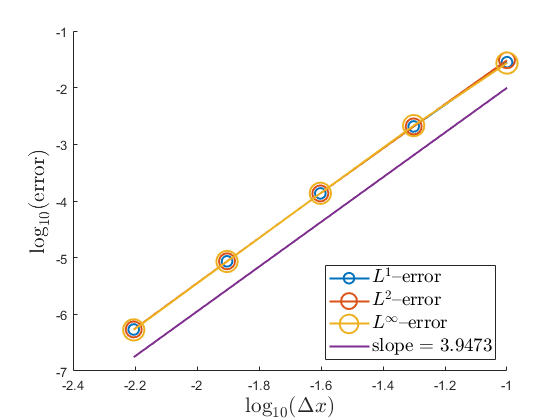
Figure 2: Accuracy error in $L^{1},L^{2},L^{\infty}$–norms, with for a fixed $\Delta t_{\rm ref}=10^{-5}$ for Eq. (17). The domain is $\Omega=[-1,1]^{2}$, $N_{\rm ref}=640$, the initial condition is defined in Eq. (64) with $x_{m_{1}}=y_{m_{1}}=0,\sigma=0.1$ and homogeneous Dirichlet boundary conditions (i.e., $f=0$ in Eq. (13)).

After some algebraic computation we have

$$c(x)=\frac{4\,c(x+2h)+4\,c(x-2h)-c(x+h)-c(x-h)}{6},$$

that at discrete levels becomes

$$c_{j}=\frac{4\,c_{j+2}+4\,c_{j-2}-c_{j+1}-c_{j-1}}{6},$$

and from this formula we can extend it to 2D, and extrapolate those values ${c}_{i,j},\{i,j\}\in\{i\in\{1,N-1\},\,\forall j\}\cup\{j\in\{1,N-1\},\,\forall i\}$. For example, regarding the operator $L^{\rm 4th}_{h}$, if $i=2$ and $j=N-1$, we have

$$L^{\rm 4th}_{h}\,c_{h}\Big{|}_{2,N-1}=\frac{1}{12h^{2}}\left(12\,c_{1,N-1}+12\,c_{3,N-1}+12\,c_{2,N-2}+12\,c_{2,N}-48\,c_{2,N-1}\right).$$

2.1.3 Fourth order space discretization with variable coefficients

In this section we add the dependence in space and time of the coefficient $u$ of the advection term, since the main interest of the paper is the description of a time oscillating motion of an obstacle (the air bubble in Fig. 1 (a)). In this case, Eq. (12) becomes

$$\frac{\partial c}{\partial t}=D\Delta c+\nabla\cdot(\vec{u}c)\quad{\rm in}\,\Omega,$$ (20)

where $\vec{u}=\vec{u}(\vec{x},t)$ is a known function.

Representing $u(\vec{x},t)$ as a column vector $\vec{u}_{h}(t)=(\ldots,\vec{u}_{i,j}(t),\ldots)^{\top}\in\mathbb{R}^{N+1}$, , where $\vec{u}_{i,j}(t)=[{u}^{x}_{i,j}(t),{u}^{y}_{i,j}(t)]$, the advection term in the problem (20) is then discretized in space, leading to a new linear system

$$\frac{\partial c_{h}}{\partial t}=L^{\rm 4th}_{h}c_{h}+{Q^{\rm 4th}_{h}}(\vec{u}_{h})c_{h}$$ (21)

where $Q_{h}^{\rm 4th}(\vec{u}_{h})$ is a $(N+1)\times(N+1)$ matrix, representing the discretization of the advection operator, and it is defined as follows

$$Q_{h}^{\rm 4th}\,\left(\vec{u}_{h}\right)\,c_{\varepsilon,h}\Big{|}_{i,j}= \begin{pmatrix}u^{x}_{i-2,j}&-8u^{x}_{i-1,j}&8u^{x}_{i+1,j}&-u^{x}_{i+2,j}\end{pmatrix}\cdot\begin{pmatrix}c_{i-2,j}\\ c_{i-1,j}\\ c_{i+1,j}\\ c_{i+2,j}\end{pmatrix}+$$ (22)

$$\begin{pmatrix}u^{y}_{i,j-2}&-8u^{y}_{i,j-1}&8u^{y}_{i,j+1}&-u^{y}_{i,j+2}\end{pmatrix}\cdot\begin{pmatrix}c_{i,j-2}\\ c_{i,j-1}\\ c_{i,j+1}\\ c_{i,j+2}\end{pmatrix},$$ (23)

where we drop the explicit dependence in time of the components of $\vec{u}_{h}$, for simplicity.

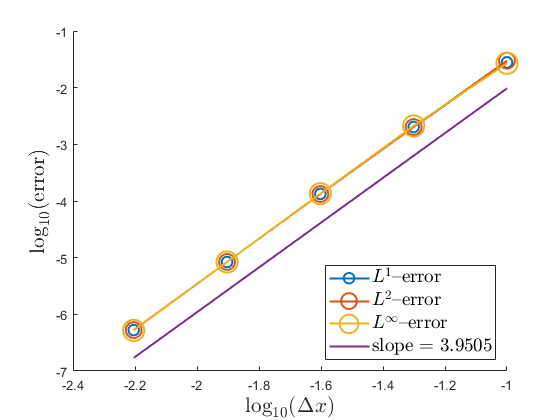
Figure 3: Accuracy error in $L^{1},L^{2},L^{\infty}$–norms, for a fixed $\Delta t_{\rm ref}=10^{-5}$ for Eq. (21). The domain is $\Omega=[-1,1]^{2}$, $N_{\rm ref}=640$, the initial condition is defined in Eq. (64) with $x_{m_{1}}=y_{m_{1}}=0$ and $\sigma=0.1$, the velocity in Eq. (63), and homogeneous Dirichlet boundary conditions (i.e., $f=0$ in Eq. (13)).

2.2 Irregular domain and ghost points

In this section, we describe the space discretization for Eqs. (8–11). The domain is
$\Omega=([-L_{x}/2,L_{x}/2]\times[-L_{y}/2,L_{y}/2])\setminus\mathcal{B}$, with $\mathcal{B}$ a circle centered in $(0,0)$ and radius $R_{\mathcal{B}}$ (see Fig. 4 (a)), and the problem reads:

$$\left\{\begin{array}[]{l}\displaystyle\frac{\partial c_{\varepsilon}}{\partial t}=D\Delta c_{\varepsilon}+\nabla\cdot(c_{\varepsilon}\vec{u}(t/\varepsilon))\quad\text{ in $\Omega$}\\ \displaystyle\nabla c_{\varepsilon}\cdot n=0\quad\text{ on $\Gamma_{\mathcal{S}}$}\\ \displaystyle\mathcal{M}\frac{\partial c_{\varepsilon}}{\partial t}=\mathcal{M}D\Delta_{\perp}c_{\varepsilon}-D\frac{\partial c_{\varepsilon}}{\partial n}\quad\text{ on $\Gamma_{\mathcal{B}}$}\end{array}\right.$$

where the expression for the velocity $\vec{u}(t/\varepsilon)=\vec{u}(x,y,t/\varepsilon)$ is known, $n$ is the outgoing normal vector to $\Gamma_{\mathcal{B}}$, and $\Delta_{\perp}={\partial^{2}}/{\partial\tau^{2}}$ denotes the Laplace–Beltrami operator on the circumference of the circle (see Fig. 4 (a)).

\begin{overpic}[abs,width=281.85034pt,unit=1mm,scale={.25}]{Figures/domains2D_squared} \put(-7.0,47.0){(a)} \put(27.5,33.5){$\tau$} \put(23.0,20.0){$\mathcal{B}$} \put(25.0,38.0){$\Omega$} \put(42.0,36.0){$\Gamma$} \put(11.0,24.0){$\Gamma_{\mathcal{B}}$} \end{overpic}

\begin{overpic}[abs,width=281.85034pt,unit=1mm,scale={.25}]{Figures/classification_points} \put(3.0,43.0){{Inactive points}} \put(3.0,46.0){{Ghost points}} \put(3.0,49.0){{Inside points}} \put(-7.0,47.0){(b)} \put(8.0,12.0){$\mathcal{B}$} \put(32.0,25.0){$\Omega$} \end{overpic}

Figure 4: (a): Representation of the domain $\Omega$ in 2D, where $\Gamma$ is the external wall, $\mathcal{B}$ is the bubble with boundary $\Gamma_{\mathcal{B}}$ and radius $R_{\mathcal{B}}$. (b): Classification of the inside (blue circles), ghost (orange circles) and inactive (red hole circles) points.

2.2.1 High order and ghost points

The space discretization of the internal points of the domain $\Omega$ (see Fig. 4 (a)) is analogue to the one of Section 2.1, with a particular attention to the boundary points close to $\Gamma_{\mathcal{B}}$. As we mentioned in the Introduction, the focus of this paper is the uniform high order time discretization, and, in Section 2.3, we introduce a third order numerical scheme. For this reason, in this section, we propose a third order accurate in space discretization for the ghost points. To obtain such an order, we need a 16–point stencil for the interpolation of the function at the ghost point $G$ in Fig. 5 (b).

Following the approach showed in [41, 42, 43, 44], the bubble $\mathcal{B}$ is implicitly defined by a level set function $\phi(x,y)$ that is positive inside the bubble, negative outside and zero on the boundary $\Gamma_{\mathcal{B}}$ :

$$\mathcal{B}=\{(x,y):\phi(x,y)>0\},\qquad\Gamma_{\mathcal{B}}=\{(x,y):\phi(x,y)=0\}.$$ (25)

The unit normal vector $n$ in (30) can be computed as $n=\frac{\nabla\phi}{|\nabla\phi|}$. For a spherical bubble $\mathcal{B}$ centered at the origin, the most convenient level–set function in terms of numerical stability is the the signed distance function between $(x,y)$ and $\Gamma_{\mathcal{B}}$, i.e. $\phi=R_{\mathcal{B}}-\sqrt{x^{2}+y^{2}}$.

After defining a uniform square Cartesian discretization, such that
${\Omega}_{h}=(x_{h},y_{h})=\{(x_{i},y_{j})=(ih,jh),(i,j)\in\{0,\cdots,N\}^{2}\}$, with $h=\Delta x=\Delta y=Lx/(N-1),\,N\in\mathbb{N}$, and the set of grid points $\mathcal{S}_{h}$, we define the set of internal points $\Omega_{h}=\mathcal{S}_{h}\cap\Omega$, the set of bubble points $\mathcal{B}_{h}=\mathcal{S}_{h}\cap\mathcal{B}$ and the set of ghost points $\mathcal{G}_{h}$, which are points that belong to $\mathcal{B}$, with at least an internal point as neighbor, and are formally defines as follows

$$(x_{i},y_{j})\in\mathcal{G}_{h}\iff(x_{i},y_{j})\in\mathcal{B}_{h}\text{ and }\{(x_{i}\pm h,y_{j}),(x_{i},y_{j}\pm h)\}\cap\Omega_{h}\neq\emptyset.$$ (26)

The other grid points, $\mathcal{S}_{h}\setminus(\Omega_{h}\cup\mathcal{G}_{h})$, are called inactive points. See Fig. 4 (b) for a classification of the different points that belong to $S_{h}$. Let $N_{I}=|\Omega_{h}|$ and $N_{G}=|\mathcal{G}_{h}|$ be the cardinality of the sets $\Omega_{h}$ and $\mathcal{G}_{h}$, respectively, and $\mathcal{N}=N_{I}+N_{G}$ the total number of active points. To compute the solution $c_{\varepsilon,h}$ at the grid points of $\Omega_{h}\cup\mathcal{G}_{h}$, we use a finite difference discretization of the equations on the $N_{I}$ internal grid points, and suitable interpolations for the $N_{G}$ ghost values, to close the system. This points play a role in the discretization of the drift and diffusion terms for the internal points, when these are in the proximity of $\Gamma_{\mathcal{B}}$. For this reason, the equations for the ghost points are coupled, and the result is a $\mathcal{N}\times\mathcal{N}$ system, with non–eliminated boundary conditions.

\begin{overpic}[abs,width=325.215pt,unit=1mm,scale={.25}]{Figures/stencil9points} \put(41.0,42.0){$\Omega$} \put(-1.0,9.0){$\mathcal{B}$} \put(-9.0,45.0){(a)} \put(4.0,49.0){j+2} \put(4.0,38.5){j+1} \put(5.0,29.0){j} \put(21.0,31.0){$P_{\rm i,j}$} \put(4.0,20.0){j-1} \put(4.0,7.5){j-2} \put(4.0,2.0){i-2} \put(14.0,2.0){i-1} \put(24.0,2.0){i} \put(35.0,2.0){i+1} \put(45.0,2.0){i+2} \end{overpic}

\begin{overpic}[abs,width=281.85034pt,unit=1mm,scale={.25}]{Figures/stencil16points} \put(10.0,14.0){\small$\vartheta_{y}h$} \put(0.0,17.0){\small$\vartheta_{x}h$} \put(-6.0,45.0){(b)} \put(31.0,18.0){$x$--interpolation} \put(31.0,15.0){$y$--interpolation} \put(31.0,11.0){Inside points} \put(31.0,8.0){Ghost points} \put(31.0,4.5){Boundary points} \put(17.0,31.0){B} \put(8.0,18.0){G} \put(4.0,43.0){$\Omega$} \put(4.0,8.0){$\mathcal{B}$} \end{overpic}

Figure 5: (a): 9–point stencil for the discrete operators $L_{{\rm i},h}^{\rm 4th}$ and $Q_{{\rm i},h}^{\rm 4th}$ of the derivatives in space for the internal points $P_{\rm i,j}=(x_{i},y_{j})$. (b): Representation of the Upwind 16–points stencil associated with the ghost point $G$, boundary point $B$ and the relative outgoing normal vector $n$ to $\Gamma$. In the figure, the stencil is composed by 15 blue internal points, together with the orange point G.

In this case, we rewrite Eq. (21) as follows

$$\partial_{t}c_{\varepsilon,h} = \left(L^{\rm 4th}_{{\rm i},h}+Q_{{\rm i},h}^{\rm 4th}(\vec{u}_{h}(t/\varepsilon))\right)c_{\varepsilon,h},\quad c^{0}_{\varepsilon,h}=c_{\varepsilon,h}(t=0),$$ (27)

where $L_{{\rm i},h}^{\rm 4th}$ and $Q_{{\rm i},h}^{\rm 4th}$ are $\mathcal{N}\times\mathcal{N}$ matrices representing the discretization of the derivative, including this time, the interpolation operators. If $P_{ij}=(x_{i},y_{j})\in\Omega_{h}$ is an internal grid point (as in Fig. 5 (a)), the expressions of $L_{{\rm i},h}^{\rm 4th}$ and $Q_{{\rm i},h}^{\rm 4th}$ coincide with of $L_{h}^{\rm 4th}$ and $Q_{h}^{\rm 4th}$. If $G=(x_{i},y_{j})\in\mathcal{G}_{h}$ is a ghost point, then we discretize the boundary condition in (10) for $\Gamma_{\mathcal{B}}$, following a ghost–point approach similar to the one proposed in [45, 46, 37, 47], where in [48] they introduce a high order discretization for the ghost points, and it is summarised as follows. We first compute the closest boundary point $B\in\Gamma_{\mathcal{B}}$ by

$$B=O+R_{\mathcal{B}}\frac{O-G}{|O-G|},$$

where $O$ is the center of the bubble. Then, we identify the upwind 16–point stencil starting from $G=(x_{G},y_{G})=(x_{i},y_{j})$, containing $B=(x_{B},y_{B})$:

$$\left\{(x_{i+s_{x}m_{x}},x_{j+s_{y}m_{y}})\colon m_{x},m_{y}=0,1,2\right\},$$

where $s_{x}=\text{SGN}(x_{B}-x_{G})$ and $s_{y}=\text{SGN}(y_{B}-y_{G})$. The solution $c_{\varepsilon,h}$ and its first and second derivatives are then interpolated at the boundary point $B$ using the discrete values $c^{\varepsilon}_{i,j}$ on the 16–point stencil. We start defining (see Fig. 5 (b))

$$\vartheta_{x}=s_{x}(x_{B}-x_{G})/h,\qquad\vartheta_{y}=s_{y}(y_{B}-y_{G})/h,$$

with $0\leq\vartheta_{x},\vartheta_{y}<1$. The 2D interpolation formulas are:

$$\widehat{c}(B)=\sum_{m_{x},m_{y}=0}^{3}l_{m_{x}}(\vartheta_{x})l_{m_{y}}(\vartheta_{y})c_{i+s_{x}m_{x},j+s_{y}m_{y}},\\ \frac{\partial\widehat{c}}{\partial x}(B)=s_{x}\sum_{m_{x},m_{y}=0}^{3}l^{\prime}_{m_{x}}(\vartheta_{x})l_{m_{y}}(\vartheta_{y})c_{i+s_{x}m_{x},j+s_{y}m_{y}},\\ \frac{\partial^{2}\widehat{c}}{\partial x^{2}}(B)=\sum_{m_{x},m_{y}=0}^{3}l^{\prime\prime}_{m_{x}}(\vartheta_{x})l_{m_{y}}(\vartheta_{y})c_{i+s_{x}m_{x},j+s_{y}m_{y}},\\ \frac{\partial^{2}\widehat{c}}{\partial x\partial y}(B)=s_{x}\,s_{y}\sum_{m_{x},m_{y}=0}^{3}l^{\prime}_{m_{x}}(\vartheta_{x})l^{\prime}_{m_{y}}(\vartheta_{y})c_{i+s_{x}m_{x},j+s_{y}m_{y}},$$ (28)

where

$$l(\vartheta_{\alpha}) =\left(\frac{1}{2}\left(1-\frac{1}{2}\vartheta_{\alpha}\right)\left(\frac{3}{2}\vartheta_{\alpha}-1\right)\left(\frac{3}{2}\vartheta_{\alpha}-2\right),\,\frac{9}{4}\vartheta_{\alpha}\left(\frac{3}{2}\vartheta_{\alpha}-2\right)\left(\frac{3}{2}\vartheta_{\alpha}-1\right),\right.$$

$$\left.\,\frac{9}{4}\vartheta_{\alpha}\left(1-\frac{3}{2}\vartheta_{\alpha}\right)\left(\frac{1}{2}\vartheta_{\alpha}-1\right),\,\frac{1}{4}\vartheta_{\alpha}\left(\frac{3}{2}\vartheta_{\alpha}-1\right)\left(\frac{3}{2}\vartheta_{\alpha}-2\right)\right),$$

$$l^{\prime}\left(\vartheta_{\alpha}\right) =\frac{1}{h}\left(-\frac{1}{6}\left(\frac{27}{4}\vartheta_{\alpha}^{2}-18\vartheta_{\alpha}+11\right),\,\frac{3}{2}\left(\frac{9}{4}\vartheta_{\alpha}^{2}-5\vartheta_{\alpha}+2\right),\right.$$

$$\left.\,-\frac{3}{2}\left(\frac{9}{4}\vartheta_{\alpha}^{2}-4\vartheta_{\alpha}+1\right),\,\frac{1}{6}\left(\frac{27}{4}\vartheta_{\alpha}^{2}-9\vartheta_{\alpha}+2\right)\right)$$

$$l^{\prime\prime}\left(\vartheta_{\alpha}\right) =\frac{1}{h^{2}}\left(-2\left(\frac{1}{2}\vartheta_{\alpha}-1\right),3\vartheta_{\alpha}-5,-2\left(\frac{3}{2}\vartheta_{\alpha}-2\right),\vartheta_{\alpha}-1\right),\quad\alpha=x,y,$$

and where we omit ${\partial\widehat{c}}/{\partial y}(B)$ and ${\partial^{2}\widehat{c}}/{\partial y^{2}}(B)$ because they are analogue to the $x-$coordinate derivatives. Finally, the rows of $L_{{\rm i},h}^{\rm 4th}$ associated with the ghost point $G=(x_{G},y_{G})$ are defined by evaluating the boundary condition on $\Gamma_{\mathcal{B}}$, i.e.

$$L_{{\rm i},h}^{\rm 4th}c_{\varepsilon,h}\Big{|}_{B}=D\left.\frac{\partial^{2}\widehat{c}}{\partial\tau^{2}}\right|_{B}-\frac{D}{\mathcal{M}}\left.\frac{\partial\widehat{c}}{\partial n}\right|_{B},$$ (29)

and

$$\frac{\partial}{\partial\tau}=\tau_{x}\,\frac{\partial}{\partial x}+\tau_{y}\,\frac{\partial}{\partial y},\quad\frac{\partial}{\partial n}=n_{x}\,\frac{\partial}{\partial x}+n_{y}\,\frac{\partial}{\partial y},$$ (30)

with $(\tau_{x},\tau_{y})=(-n_{y},n_{x})$, $\cot\theta=n_{x}/n_{y}$. For a spherical bubble,
$(n_{x},n_{y})=({O-G})/{|O-G|},\,\>\cot\theta=x/y$.

2.3 Time discretization

In this section, we construct a scheme to solve Eq. (21), that is uniformly accurate in $\varepsilon$. The only property that we use is that the first time derivative of the solution is uniformly bounded in $\varepsilon$, and this property is justified since we assume that the initial condition is not oscillatory in space and the boundary conditions for the concentration are not oscillatory in time.

As we mentioned in the Introduction, in this section we start defining a numerical scheme that is first order accurate in time, and, recursively, we obtain second and third order numerical schemes. This paper is a natural continuation of a previous one [29], where first and second order schemes are already defined. Here, we recall them to show the technique to derive the third order scheme.

Proposition 1.

Let ${L^{\rm 4th}_{h}}$ and ${Q^{\rm 4th}_{h}}$ be bounded operators in $\mathbb{R}^{\mathcal{N}}$ defined in Section 2.1.2, with $h>0$. Let $c_{\varepsilon,h}^{0}\in\mathbb{R}^{\mathcal{N}}$ be bounded in $\varepsilon$, $\vec{u}_{h}\in\mathbb{R}^{\mathcal{N}}$ be a bounded given $1-$periodic function of time. Then, there exists a constant $\Delta t_{0}>0$ independent of $\varepsilon$ such that, for all $\Delta t<\Delta t_{0}$, the following holds true:

• The operator $\mathcal{A}^{1}_{\Delta t}:=I-\Delta t{L^{\rm 4th}_{h}}-{Q^{\rm 4th}_{h}}\int_{t^{n}}^{t^{n+1}}\vec{u}_{h}(s/\varepsilon)\,ds$ in $\mathbb{R}^{\mathcal{N}}$ is invertible.

• The following:

  $$c_{\varepsilon,h}^{0} = c_{\varepsilon,h}(0),$$ (31)

  $$c_{\varepsilon,h}^{n+1} = {\mathcal{A}^{1}_{\Delta t}}^{-1}c_{\varepsilon,h}^{n},$$ (32)

  for $n=1,\cdots,M$ is a first order scheme, uniformly accurate with respect to $\varepsilon$, solving the Eq. (21). In other words, we have $||c_{\varepsilon,h}(t^{n})-c_{\varepsilon,h}^{n}||\leq K\Delta t$ for all $n=1,\cdots,M$, with $K$ independent of $\varepsilon$, $\Delta t=t_{\rm fin}/M$, $t_{\rm fin}>0$ and $t^{n}=n\Delta t$.

The same result is valid also for the Eq. (27), where the operators are $L^{\rm 4th}_{{\rm i},h}$ and $Q^{\rm 4th}_{{\rm i},h}$, and the proof is analogue.

Proof.

To prove i), we first show that $\mathcal{A}^{1}_{\Delta t}\to I$, when $\Delta t\to 0$ since the operators ${L^{\rm 4th}_{h}}$ and ${Q^{\rm 4th}_{h}}$, and the function $\vec{u}_{h}$ are bounded. Thus, there exists a constant $\widehat{K}>0$ (independent of $\varepsilon$), such that, $\forall\Delta t<\widehat{K}$, ${\rm det}(\mathcal{A}^{1}_{\Delta t})\neq 0$, and $\mathcal{A}^{1}_{\Delta t}$ is invertible.

To prove ii), we first show how to deduce the scheme defined in Eqs. (31–32). We start integrating Eq. (21) between $t$ and $t^{n+1}$, with $[t,t^{n+1}]\subset[t^{n},t_{\rm fin}]$

$$c_{\varepsilon,h}(t^{n+1})-c_{\varepsilon,h}(t) = \int_{t}^{t^{n+1}}\left({L^{\rm 4th}_{h}}+{Q^{\rm 4th}_{h}}\vec{u}_{h}(s/\varepsilon)\right)c_{\varepsilon,h}(s)ds.$$ (33)

Evaluating the quantity $c_{\varepsilon,h}(t)$ in $t=t^{n}$, we obtain

$$c_{\varepsilon,h}(t^{n+1})-c_{\varepsilon,h}(t^{n}) = \int_{t^{n}}^{t^{n+1}}\left({L^{\rm 4th}_{h}}+{Q^{\rm 4th}_{h}}\vec{u}_{h}(s/\varepsilon)\right)c_{\varepsilon,h}(s)ds,$$ (34)

and then the following

$$c_{\varepsilon,h}(t^{n+1})-c_{\varepsilon,h}(t^{n})\approx\left(\int_{t^{n}}^{t^{n+1}}\left({L^{\rm 4th}_{h}}+{Q^{\rm 4th}_{h}}\vec{u}_{h}(s/\varepsilon)\right)\,ds\right)c_{\varepsilon,h}(t^{n+1}).$$ (35)

Since the operators ${L^{\rm 4th}_{h}}$ and ${Q^{\rm 4th}_{h}}$ do not depend on time, Eq. (35) becomes

$$c_{\varepsilon,h}(t^{n+1})-c_{\varepsilon,h}(t^{n})\approx{L^{\rm 4th}_{h}}\,\Delta tc_{\varepsilon,h}(t^{n+1})+{Q^{\rm 4th}_{h}}c_{\varepsilon,h}(t^{n+1})\int_{t^{n}}^{t^{n+1}}\vec{u}_{h}(s/\varepsilon)ds$$ (36)

where the integral $\int_{t^{n}}^{t^{n+1}}\vec{u}_{h}(s/\varepsilon)\,ds$ is calculated analytically. At the end, the scheme reads

$$c_{\varepsilon,h}^{n+1}-c_{\varepsilon,h}^{n}={L^{\rm 4th}_{h}}\,\Delta t\,c_{\varepsilon,h}^{n+1}+{Q^{\rm 4th}_{h}}c_{\varepsilon,h}^{n+1}\int_{t^{n}}^{t^{n+1}}\vec{u}_{h}(s/\varepsilon)\,ds$$ (37)

where $c_{\varepsilon,h}^{n}\approx c_{\varepsilon,h}(t^{n})$.

Now, we prove that the scheme in Eq. (37) is first order in $\Delta t$, uniformly in $\varepsilon$. We subtract Eq. (37) from Eq. (34), define the error at time $t^{n}$ as $e_{n}=c_{\varepsilon,h}(t^{n})-c_{\varepsilon,h}^{n}$, and obtain

$$e_{n+1}-e_{n}=\int_{t^{n}}^{t^{n+1}}\left({L^{\rm 4th}_{h}}+{Q^{\rm 4th}_{h}}\vec{u}_{h}(s/\varepsilon)\right)\left(c_{\varepsilon,h}(s)-c_{\varepsilon,h}^{n+1}\right)\,ds.$$ (38)

Here we substitute $\,c_{\varepsilon,h}(s)-c_{\varepsilon,h}^{n+1}=c_{\varepsilon,h}(s)-c_{\varepsilon,h}(t^{n+1})+c_{\varepsilon,h}(t^{n+1})-c_{\varepsilon,h}^{n+1}\,$ in Eq. (38), obtaining

$$e_{n+1}-e_{n} = \displaystyle\int_{t^{n}}^{t^{n+1}}\left({L^{\rm 4th}_{h}}+{Q^{\rm 4th}_{h}}\vec{u}_{h}(s/\varepsilon)\right)\left(c_{\varepsilon,h}(s)-c_{\varepsilon,h}(t^{n+1})\right)\,ds$$ (39)

$$\displaystyle+\int_{t^{n}}^{t^{n+1}}\left({L^{\rm 4th}_{h}}+{Q^{\rm 4th}_{h}}\vec{u}_{h}(s/\varepsilon)\right)\,ds\left(c_{\varepsilon,h}(t^{n+1})-c_{\varepsilon,h}^{n+1}\right).$$

Since $\vec{u}_{h}(t/\varepsilon)$ and $c_{\varepsilon,h}(t)$ are bounded, also the first derivative in time of $c_{\varepsilon,h}(t)$ is bounded, i.e., there exists a constant $K_{1}$, independent of $\varepsilon$, such that

$$||\partial_{t}c_{\varepsilon,h}||_{\mathcal{L}^{\infty}(\Omega)}=||\left({L^{\rm 4th}_{h}}+{Q^{\rm 4th}_{h}}\vec{u}_{h}(t/\varepsilon)\right)c_{\varepsilon,h}||_{\mathcal{L}^{\infty}(\Omega)}<K_{1}.$$

where $K_{1}=\left(||{L^{\rm 4th}_{h}}||+||{Q^{\rm 4th}_{h}}||\,||u||_{\infty}\right)||c_{\varepsilon,h}||_{\mathcal{L}^{\infty}(\Omega)}$. From this estimate, we obtain

$$||c_{\varepsilon,h}(s)-c_{\varepsilon,h}(t^{n+1})||\leq K_{1}||s-t^{n+1}||\leq K_{1}\Delta t,\qquad\forall s\in[t^{n},t^{n+1}].$$ (40)

Now we consider the first term of the RHS of Eq. (39), that is bounded by

$$\left|\left|\int_{t^{n}}^{t^{n+1}}\left({L^{\rm 4th}_{h}}+{Q^{\rm 4th}_{h}}\vec{u}_{h}(s/\varepsilon)\right)\left(c_{\varepsilon,h}(s)-c_{\varepsilon,h}(t^{n+1})\right)\,ds\right|\right|\leq K_{1}K_{2}\Delta t^{2}$$ (41)

where $K_{2}=||{L^{\rm 4th}_{h}}+{Q^{\rm 4th}_{h}}\vec{u}_{h}(s/\varepsilon)||_{\mathcal{L}^{\infty}(\Omega)}$, and, it does not depend on $\varepsilon$.

Considering now the norm of the Eq. (39), the following inequalities hold

$$||e_{n+1}||-||e_{n}||\leq||e_{n+1}-e_{n}||\leq K_{1}K_{2}\Delta t^{2}+||e_{n+1}||K_{2}\Delta t\leq K_{3}\Delta t^{2}+||e_{n+1}||K_{3}\Delta t,$$ (42)

where $K_{3}=\max\{K_{1}K_{2},K_{2}\}$. After some algebra, adding $\Delta t$ in both sides, and defining $E_{n}=||e_{n}||$, we have

$$E_{n+1}+\Delta t\leq(1-K_{3}\Delta t)^{-1}(E_{n}+\Delta t).$$ (43)

if, and only if, $\Delta t<1/K_{3}$. From Eq. (43), recursively to $E_{0}=0$, we obtain that

$$E_{n}+\Delta t\leq(1-K_{3}\Delta t)^{-n}\Delta t\leq\left(1-K_{3}\frac{t_{\rm fin}}{N}\right)^{-N}\Delta t$$

which follows that, there exists a constant $K_{4}$, such that

$$E_{n}\leq\left(\left(1-K_{3}\frac{t_{\rm fin}}{N}\right)^{-N}-1\right)\Delta t\leq K_{4}\Delta t$$

$K_{4}$ independent of $N$, since $\lim_{N\to+\infty}\left(\left(1-K_{3}\,{t_{\rm fin}}/{N}\right)^{-N}-1\right)=\exp{(K_{3}t_{\rm fin})}-1$.
To conclude the proof, we define $\Delta t_{0}=\min\{\widehat{K},1/K_{3}\}.$ ∎

Proposition 2.

Let ${L^{\rm 4th}_{h}}$ and ${Q^{\rm 4th}_{h}}$ be finite dimensional bounded operators in $\mathbb{R}^{\mathcal{N}}$ defined in Section 2.1.2, with $h>0$. Let $c_{\varepsilon,h}^{0}\in\mathbb{R}^{\mathcal{N}}$ be bounded in $\varepsilon$, and let $\vec{u}_{h}\in\mathbb{R}^{\mathcal{N}}$ be a bounded given $1-$periodic function in time. Then, there exists a constant $\Delta t_{0}>0$ independent of $\varepsilon$, such that for all $\Delta t<\Delta t_{0}$, the following holds true:

• The operator $\mathcal{A}^{2}_{\Delta t}=\mathcal{A}^{1}_{\Delta t}-\mathbb{M}_{2}$ in $\mathbb{R}^{\mathcal{N}}$ is invertible, where

  $$\mathbb{M}_{2}=-\frac{1}{2}\left(L^{\rm 4th}_{h}\right)^{2}\Delta t^{2}-{L^{\rm 4th}_{h}}{Q^{\rm 4th}_{h}}\int_{t^{n}}^{t^{n+1}}\int_{s}^{t^{n+1}}\vec{u}_{h}(\sigma/\varepsilon)\,d\sigma ds$$

  $$-{Q^{\rm 4th}_{h}}{L^{\rm 4th}_{h}}\int_{t^{n}}^{t^{n+1}}(t^{n+1}-s)\vec{u}_{h}(s/\varepsilon)\,ds$$

  $$-\left(Q^{\rm 4th}_{h}\right)^{2}\int_{t^{n}}^{t^{n+1}}\vec{u}_{h}(s/\varepsilon)\int_{s}^{t^{n+1}}\vec{u}_{h}(\sigma/\varepsilon)\,d\sigma\,ds,$$

• The following scheme:

  $$c_{\varepsilon,h}^{0} = c_{\varepsilon,h}(0),$$ (44)

  $$c_{\varepsilon,h}^{n+1} = {\mathcal{A}^{2}_{\Delta t}}^{-1}c_{\varepsilon,h}^{n},\qquad{\rm for}\quad n=1,\cdots,M$$ (45)

  is a second order scheme, uniformly accurate with respect to $\varepsilon$, solving the Eq. (21). In other words we have $||c_{h}(t^{n})-c_{h}^{n}||\leq K\Delta t^{2}$, for all $n=1,\cdots,M$, with $K$ independent of $\varepsilon$, $t^{n}=n\Delta t$ and $\Delta t=t_{\rm fin}/M$.

We skip the proof of the second order scheme because it is analogue to the one for the first order, and it is valid also for the Eq. (27). Anyway, it can be found in [29, Proposition 2].

Proposition 3.

Let ${L^{\rm 4th}_{h}}$ and ${Q^{\rm 4th}_{h}}$ be finite dimensional bounded operators in $\mathbb{R}^{\mathcal{N}}$ defined in Section 2.1.2, with $h>0$. Let $c_{\varepsilon,h}^{0}\in\mathbb{R}^{\mathcal{N}}$ be bounded in $\varepsilon$, and let $\vec{u}_{h}\in\mathbb{R}^{\mathcal{N}}$ be a bounded given $1-$periodic function in time. Then, there exists a constant $\Delta t_{0}>0$ independent of $\varepsilon$, such that for all $\Delta t<\Delta t_{0}$, the following holds true:

• The operator $\mathcal{A}^{3}_{\Delta t}=\mathcal{A}^{2}_{\Delta t}-\mathbb{M}_{3}$ in $\mathbb{R}^{\mathcal{N}}$ is invertible, where

  $$\mathbb{M}_{3} =\frac{1}{2}\left(L^{\rm 4th}_{h}\right)^{3}\int_{t^{n}}^{t^{n+1}}(t^{n+1}-s)^{2}\,ds$$

  $$+\left(L^{\rm 4th}_{h}\right)^{2}{Q^{\rm 4th}_{h}}\int_{t^{n}}^{t^{n+1}}\int_{s}^{t^{n+1}}\int_{\sigma}^{t^{n+1}}\vec{u}_{h}(\rho/\varepsilon)d\rho\,d\sigma$$

  $$+{L^{\rm 4th}_{h}}{Q^{\rm 4th}_{h}}{L^{\rm 4th}_{h}}\int_{t^{n}}^{t^{n+1}}\int_{s}^{t^{n+1}}(t^{n+1}-\sigma)\vec{u}_{h}(\sigma/\varepsilon)d\sigma ds$$

  $$+{L^{\rm 4th}_{h}}\left(Q^{\rm 4th}_{h}\right)^{2}\int_{t^{n}}^{t^{n+1}}\int_{s}^{t^{n+1}}\vec{u}_{h}(\sigma/\varepsilon)\int_{\sigma}^{t^{n+1}}\vec{u}_{h}(\rho/\varepsilon)d\rho\,d\sigma\,ds$$

  $$+\frac{1}{2}{Q^{\rm 4th}_{h}}\left(L^{\rm 4th}_{h}\right)^{2}\int_{t^{n}}^{t^{n+1}}(t^{n+1}-s)^{2}\vec{u}_{h}(s/\varepsilon)ds$$

  $$+{Q^{\rm 4th}_{h}}{L^{\rm 4th}_{h}}{Q^{\rm 4th}_{h}}\int_{t^{n}}^{t^{n+1}}\vec{u}_{h}(s/\varepsilon)\int_{s}^{t^{n+1}}\int_{\sigma}^{t^{n+1}}\vec{u}_{h}(\rho/\varepsilon)d\rho\,d\sigma\,ds$$

  $$+\left(Q^{\rm 4th}_{h}\right)^{2}{L^{\rm 4th}_{h}}\int_{t^{n}}^{t^{n+1}}\vec{u}_{h}(s/\varepsilon)\int_{s}^{t^{n+1}}(t^{n+1}-\sigma)\vec{u}_{h}(\sigma/\varepsilon)d\sigma\,ds$$

  $$+\left(Q^{\rm 4th}_{h}\right)^{3}\int_{t^{n}}^{t^{n+1}}\vec{u}_{h}(s/\varepsilon)\int_{s}^{t^{n+1}}\vec{u}_{h}(\sigma/\varepsilon)\int_{\sigma}^{t^{n+1}}\vec{u}_{h}(\rho/\varepsilon)d\rho\,d\sigma\,ds$$

• The following scheme:

  $$c_{\varepsilon,h}^{0} = c_{\varepsilon,h}(0),$$ (46)

  $$c_{\varepsilon,h}^{n+1} = {\mathcal{A}^{3}_{\Delta t}}^{-1}c_{\varepsilon,h}^{n},\qquad{\rm for}\quad n=1,\cdots,M$$ (47)

  is a third order scheme, uniformly accurate with respect to $\varepsilon$, solving the Eq. (21). In other words we have $||c_{h}(t^{n})-c_{h}^{n}||\leq K\Delta t^{3}$, for all $n=1,\cdots,M$, with $K$ independent of $\varepsilon$, $t^{n}=n\Delta t$ and $\Delta t=t_{\rm fin}/M$.

The same result is valid also for the Eq. (27), where the operators are $L^{\rm 4th}_{{\rm i},h}$ and $Q^{\rm 4th}_{{\rm i},h}$, and the proof is analogue.

Proof.

To prove i), we prove that $\mathcal{A}^{3}_{\Delta t}$ is invertible when $\Delta t\to 0$. We start considering the norm of the operator $\mathcal{A}^{3}_{\Delta t}$ as before, and, analogously, since the operators ${L^{\rm 4th}_{h}}$ and ${Q^{\rm 4th}_{h}}$ are bounded in $\mathbb{R}^{\mathcal{N}}$, and the vector–valued function $\vec{u}_{h}$ is also bounded, it follows that $||\mathcal{A}^{3}_{\Delta t}||\to||I||$ when $\Delta t\to 0$. Thus, following the same procedure as before, we say that there exists a constant $\widehat{K}>0$, such that, $\forall\Delta t<\widehat{K}$, the operator $\mathcal{A}^{3}_{\Delta t}$ is invertible.

To prove ii), we first show how to deduce the scheme defined in Eqs. (46–47). As before, we start integrating Eq. (21) between $t$ and $t^{n+1}$, with $[t,t^{n+1}]\subset[t^{n},t_{\rm fin}]$

$$c_{\varepsilon,h}(t^{n+1})-c_{\varepsilon,h}(t) = \int_{t}^{t^{n+1}}\left({L^{\rm 4th}_{h}}+{Q^{\rm 4th}_{h}}\vec{u}_{h}(s/\varepsilon)\right)c_{\varepsilon,h}(s)ds.$$ (48)

that can be rewritten as

$$c_{\varepsilon,h}(s)=c_{\varepsilon,h}(t^{n+1})-\int_{s}^{t^{n+1}}\left({L^{\rm 4th}_{h}}+{Q^{\rm 4th}_{h}}\vec{u}_{h}(\sigma/\varepsilon)\right)c_{\varepsilon,h}(\sigma)d\sigma.$$ (49)

Now we substitute $c_{\varepsilon,h}(s)$ in Eq. (48) with Eq. (49), as follows

$$c_{\varepsilon,h}(t^{n+1})-c_{\varepsilon,h}(t) = \int_{t}^{t^{n+1}}\left({L^{\rm 4th}_{h}}+{Q^{\rm 4th}_{h}}\vec{u}_{h}(s/\varepsilon)\right)c_{\varepsilon,h}(s)ds$$

$$= \int_{t}^{t^{n+1}}\left({L^{\rm 4th}_{h}}+{Q^{\rm 4th}_{h}}\vec{u}_{h}(s/\varepsilon)\right)\,ds\,c_{\varepsilon,h}(t^{n+1})$$

$$-\int_{t}^{t^{n+1}}\left({L^{\rm 4th}_{h}}+{Q^{\rm 4th}_{h}}\vec{u}_{h}(s/\varepsilon)\right)\int_{s}^{t^{n+1}}\left({L^{\rm 4th}_{h}}+{Q^{\rm 4th}_{h}}\vec{u}_{h}(\sigma/\varepsilon)\right)c_{\varepsilon,h}(\sigma)d\sigma\,ds.$$

Since the high order in this numerical scheme is achieved recursively, we write the analogue expression in Eq. (49), but this time for $c_{\varepsilon,h}(\sigma)$,

$$c_{\varepsilon,h}(\sigma)=c_{\varepsilon,h}(t^{n+1})-\int_{\sigma}^{t^{n+1}}\left({L^{\rm 4th}_{h}}+{Q^{\rm 4th}_{h}}\vec{u}_{h}(\rho/\varepsilon)\right)c_{\varepsilon,h}(\rho)d\rho,$$ (51)

and, analogously, we substitute $c_{\varepsilon,h}(\sigma)$ in Eq. (2.3) with Eq. (51), obtaining

$$c_{\varepsilon,h}(t^{n+1})-c_{\varepsilon,h}(t) =$$

$$=\int_{t}^{t^{n+1}}\left({L^{\rm 4th}_{h}}+{Q^{\rm 4th}_{h}}\vec{u}_{h}(s/\varepsilon)\right)\,ds\,c_{\varepsilon,h}(t^{n+1})$$

$$-\int_{t}^{t^{n+1}}\left({L^{\rm 4th}_{h}}+{Q^{\rm 4th}_{h}}\vec{u}_{h}(s/\varepsilon)\right)\int_{s}^{t^{n+1}}\left({L^{\rm 4th}_{h}}+{Q^{\rm 4th}_{h}}\vec{u}_{h}(\sigma/\varepsilon)\right)d\sigma\,ds\,c_{\varepsilon,h}(t^{n+1})$$

$$+\int_{t}^{t^{n+1}}\left({L^{\rm 4th}_{h}}+{Q^{\rm 4th}_{h}}\vec{u}_{h}(s/\varepsilon)\right)\int_{s}^{t^{n+1}}\left({L^{\rm 4th}_{h}}+{Q^{\rm 4th}_{h}}\vec{u}_{h}(\sigma/\varepsilon)\right)$$

$$\cdot\int_{\sigma}^{t^{n+1}}\left({L^{\rm 4th}_{h}}+{Q^{\rm 4th}_{h}}\vec{u}_{h}(\rho/\varepsilon)\right)c_{\varepsilon,h}(\rho)d\rho\,d\sigma\,ds.$$

At this step, we evaluate the quantity $c_{\varepsilon,h}(t)$ in $t=t^{n}$, and approximate the quantities in the following way

$$c_{\varepsilon,h}^{n+1}-c_{\varepsilon,h}^{n}= \int_{t^{n}}^{t^{n+1}}\left({L^{\rm 4th}_{h}}+{Q^{\rm 4th}_{h}}\vec{u}_{h}(s/\varepsilon)\right)\,ds\,c_{\varepsilon,h}^{n+1}$$

$$-\int_{t^{n}}^{t^{n+1}}\left({L^{\rm 4th}_{h}}+{Q^{\rm 4th}_{h}}\vec{u}_{h}(s/\varepsilon)\right)\int_{s}^{t^{n+1}}\left({L^{\rm 4th}_{h}}+{Q^{\rm 4th}_{h}}\vec{u}_{h}(\sigma/\varepsilon)\right)d\sigma\,ds\,c_{\varepsilon,h}^{n+1}$$

$$+\int_{t^{n}}^{t^{n+1}}\left({L^{\rm 4th}_{h}}+{Q^{\rm 4th}_{h}}\vec{u}_{h}(s/\varepsilon)\right)\int_{s}^{t^{n+1}}\left({L^{\rm 4th}_{h}}+{Q^{\rm 4th}_{h}}\vec{u}_{h}(\sigma/\varepsilon)\right)$$

$$\cdot\int_{\sigma}^{t^{n+1}}\left({L^{\rm 4th}_{h}}+{Q^{\rm 4th}_{h}}\vec{u}_{h}(\rho/\varepsilon)\right)d\rho\,d\sigma\,ds\,c_{\varepsilon,h}^{n+1}.$$

where $c^{n}_{\varepsilon,h}\approx c_{\varepsilon,h}(t^{n})$.

At this point, we show that the numerical scheme is third order accurate in time, uniformly in $\varepsilon$. Here we subtract Eq. (2.3) from Eq. (2.3), as before, obtaining

$$e^{n+1}-e^{n}= \int_{t^{n}}^{t^{n+1}}\left({L^{\rm 4th}_{h}}+{Q^{\rm 4th}_{h}}\vec{u}_{h}(s/\varepsilon)\right)e_{n+1}\,ds$$

$$-\int_{t^{n}}^{t^{n+1}}\left({L^{\rm 4th}_{h}}+{Q^{\rm 4th}_{h}}\vec{u}_{h}(s/\varepsilon)\right)\int_{s}^{t^{n+1}}\left({L^{\rm 4th}_{h}}+{Q^{\rm 4th}_{h}}\vec{u}_{h}(\sigma/\varepsilon)\right)e_{n+1}\,d\sigma\,ds$$

$$+\int_{t^{n}}^{t^{n+1}}\left({L^{\rm 4th}_{h}}+{Q^{\rm 4th}_{h}}\vec{u}_{h}(s/\varepsilon)\right)\int_{s}^{t^{n+1}}\left({L^{\rm 4th}_{h}}+{Q^{\rm 4th}_{h}}\vec{u}_{h}(\sigma/\varepsilon)\right)$$

$$\cdot\int_{\sigma}^{t^{n+1}}\left({L^{\rm 4th}_{h}}+{Q^{\rm 4th}_{h}}\vec{u}_{h}(\rho/\varepsilon)\right)(c_{\varepsilon,h}(\rho)-c_{\varepsilon,h}^{n+1})d\rho d\sigma ds.$$

where, again, $e_{n}=c_{\varepsilon,h}(t^{n})-c_{\varepsilon,h}^{n}$. Now we add and subtract the same quantity to the RHS, saying that, $\,c_{\varepsilon,h}(\rho)-c_{\varepsilon,h}^{n+1}=c_{\varepsilon,h}(\rho)-c_{\varepsilon,h}(t^{n+1})+c_{\varepsilon,h}(t^{n+1})-c_{\varepsilon,h}^{n+1}\,$ and, using the analogue procedure and the same constants seen in Eq. (42), Eq. (2.3) becomes

$$\left(1-K_{3}\Delta t-K_{3}^{2}\Delta t^{2}-K_{3}^{3}\Delta t^{3}\right)E_{n+1}-K_{3}^{3}\Delta t^{4}\leq E_{n}$$

where $E_{n}=||e_{n}||$. In this case, we add ${K_{3}^{2}\Delta t^{3}}/({1+K_{3}\Delta t+K_{3}^{2}\Delta t^{2}})$ to both sides, and, after some algebra, the inequality reads

$$E_{n+1}+\frac{K_{3}^{2}\Delta t^{3}}{1+K_{3}\Delta t+K_{3}^{2}\Delta t^{2}}\leq$$ (55)

$$\left(1-K_{3}\Delta t-K_{3}^{2}\Delta t^{2}-K_{3}^{3}\Delta t^{3}\right)^{-1}\left(E_{n}+\frac{K_{3}^{2}\Delta t^{3}}{1+K_{3}\Delta t+K_{3}^{2}\Delta t^{2}}\right),$$ (56)

if $K_{3}\Delta t(1+K_{3}\Delta t+K_{3}^{2}\Delta t^{2})<1$. Recursively, we obtain (using $E_{0}=0$)

$$E_{n+1}+\frac{K_{3}^{2}\Delta t^{3}}{1+K_{3}\Delta t+K_{3}^{2}\Delta t^{2}}\leq\left(1-K_{3}\Delta t-K_{3}^{2}\Delta t^{2}-K_{3}^{3}\Delta t^{3}\right)^{-n}\frac{K_{3}^{2}\Delta t^{3}}{1+K_{3}\Delta t+K_{3}^{2}\Delta t^{2}}.$$

As before, it is easy to show that there exists a constant $\widehat{K}$ that does not depend on $N$, such that $E_{n}\leq\widehat{K}\Delta t^{3}$. To conclude the proof, we define $\Delta t_{0}=\min\{\widehat{K},\widetilde{K}\}$, where $\widetilde{K}$ is the positive solution of the equation $1-K_{3}\Delta t-K_{3}^{2}\Delta t^{2}-K_{3}^{3}\Delta t^{3}=0$. ∎

\begin{overpic}[abs,width=433.62pt,unit=1mm,scale={.25}]{Figures/accuracy_time_dt_Dh_Th_3th.png} \put(0.0,47.0){(a)} \end{overpic}

\begin{overpic}[abs,width=433.62pt,unit=1mm,scale={.25}]{Figures/accuracy_epsilon_dt_plot.png} \put(0.0,47.0){(b)} \end{overpic}

Figure 6: Plot of the relative $L^{2}$ error for the third order scheme in Eqs. (46–47) as a function of $\Delta t$ and different $\varepsilon$ (a) and as a function of $\varepsilon$ and different $\Delta t$ (b). The parameters of the tests are: $t_{\rm fin}=0.1,\Delta t_{\rm ref}=10^{-5},N_{\rm ref}=160,D=0.02,\delta=10^{-2}$. The domain is $\Omega=[-1,1]^{2}$, the initial condition is defined in Eq. (64) with $x_{m_{1}}=y_{m_{1}}=0$ and $\sigma=0.1$, and the velocity expression in Eq. (66), $A=1$.

3 Numerical results

In this section we show the accuracy tests of the different numerical schemes that we derived in the previous sections. The domain considered in the following tests is $\Omega=\left([-1,1]\times[-1,1]\right)$. We start with the second and fourth order accurate in space numerical schemes for the drift–diffusion equation in Eq. (17), and for the one with variable coefficients for the drift term in Eq. (21). To conclude the accuracy tests of the space discretization, we test the third order accuracy of the numerical scheme defined in Eq. (27). In this case, the domain considered in the following tests is $\Omega=\left([-1,1]\times[-1,1]\right)\setminus\mathcal{B}$, where $\mathcal{B}$ is a circle centered in $(0,0)$ with radius $R_{\mathcal{B}}=0.2$. For the squared external boundaries, we choose homogeneous Dirichlet boundary conditions, i.e., $f=0$ in Eq. (13).

After this, we show the numerical tests for the third order accurate in time discretization, obtained in a recursive way from the lower order schemes. We focus on the uniformly accuracy in $\varepsilon$ of the numerical method, and after that, we show the advantages of the arbitrariness of choosing the time step $\Delta t$, without losing accuracy.

In Fig. 2 we show the fourth order space accuracy of the numerical scheme defined in Eq. (17). To calculate the error, we add an artificial term at the numerical scheme in (17), as follows

$$\displaystyle\frac{c_{h}^{n+1}-c_{h}^{n}}{\Delta t}= \frac{1}{2}\left(L^{\rm 4th}_{h}+D_{h}^{\rm 4th}\right)(c_{h}^{n}+c_{h}^{n+1})$$ (57)

$$+\frac{1}{2}F(c^{\rm exa}(x_{h},y_{h},t^{n}))+F(c^{\rm exa}(x_{h},y_{h},t^{n+1}))$$

where the time derivative is discretized with a second order Crank–Nicolson method, with $c_{h}^{n+1}\approx c_{h}(t^{n+1})$, the expression of $F$ is the following

$$F(c^{\rm exa}(x,y,t))=\frac{\partial}{\partial t}c^{\rm exa}(x,y,t)-\Delta\,c^{\rm exa}(x,y,t)-u\nabla\cdot c^{\rm exa}(x,y,t).$$ (58)

and the one for the manufactured exact solution is

$$\displaystyle c_{h}^{\rm exa}(t)= \cos(t)\exp\left(-\frac{(x-x_{m_{1}})^{2}+(y-y_{m_{1}})^{2}}{2\sigma^{2}}\right)$$ (59)

$$+\sin(t)\exp\left(-\frac{(x-x_{m_{2}})^{2}+(y-y_{m_{2}})^{2}}{2\sigma^{2}}\right)$$

After defining the expression of $F$, we calculate the following error

$${\rm error}_{\alpha}=\frac{||c_{h}(t_{\rm fin})-c^{\rm exa}(x_{h},y_{h},t)||_{\alpha}}{||c^{\rm exa}(x_{h},y_{h},t)||_{\alpha}}$$ (60)

where $\alpha=1,2,\infty$ indicates which norm we are considering. In Fig. 2 and in Table 1 we show the numerical error of the space discretization in Eq. (17) and the slope is $\approx 3.95$.

N	${\rm error}_{1}$	${\rm error}_{2}$	${\rm error}_{\infty}$	order
10	2.815$\cdot 10^{-2}$	3.049$\cdot 10^{-2}$	2.718$\cdot 10^{-2}$	–
20	2.069$\cdot 10^{-3}$	2.073$\cdot 10^{-3}$	2.140$\cdot 10^{-3}$	3.77
40	1.363$\cdot 10^{-4}$	1.362$\cdot 10^{-4}$	1.367$\cdot 10^{-4}$	3.92
80	8.630$\cdot 10^{-6}$	8.630$\cdot 10^{-6}$	8.589$\cdot 10^{-6}$	3.98
160	5.407$\cdot 10^{-7}$	5.409$\cdot 10^{-7}$	5.320$\cdot 10^{-7}$	4

Table 1: Convergence rate of the spatial numerical discretization defined in Eq. (17). The error is calculated in $L^{1},L^{2},L^{\infty}$–norms, for a fixed $\Delta t_{\rm ref}=10^{-5}$. The domain is $\Omega=[-1,1]^{2}$, the initial condition is defined in Eq. (64) with $x_{m_{1}}=y_{m_{1}}=0,\sigma=0.1$ and homogeneous Dirichlet boundary conditions (i.e., $f=0$ in Eq. (13)).

Analogously, in Fig. 3, we show the order of accuracy of the space discretization in Eq. (21). In this case, to calculate the solution at final time we consider the following

$$\displaystyle\frac{c_{h}^{n+1}-c_{h}^{n}}{\Delta t}= \frac{1}{2}\left(L^{\rm 4th}_{h}+Q_{h}^{\rm 4th}\right)(c_{h}^{n}+c_{h}^{n+1})$$ (61)

$$+\frac{1}{2}F(c^{\rm exa}(x_{h},y_{h},t^{n}))+F(c^{\rm exa}(x_{h},y_{h},t^{n+1})).$$

In this case, the expression for $F$ is

$$F(c_{h}^{\rm exa}(x,y,t))=\frac{\partial}{\partial t}c_{h}^{\rm exa}(x,y,t)-\Delta\,c_{h}^{\rm exa}(x,y,t)-\nabla\cdot(\vec{u}_{h}\,c_{h}^{\rm exa}(x,y,t)),$$ (62)

and the expression for $c^{\rm exa}$ is in Eq. (59). Here we define the expression of the two components of the velocity vector

$$u^{x}=x^{3},\quad u^{y}=y^{3},$$ (63)

and the initial condition

$$c_{h}^{0}=c_{h}(t=0)=\exp\left(-\frac{(x-x_{m_{1}})^{2}+(y-y_{m_{1}})^{2}}{2\sigma^{2}}\right)\equiv c_{h}^{\rm exa}(t=0),$$ (64)

and in Fig. 3 and Table 2 we show the numerical error of the space discretization in Eq. (21), and the slope is $\approx 3.95$.

N	${\rm error}_{1}$	${\rm error}_{2}$	${\rm error}_{\infty}$	order
10	2.800$\cdot 10^{-2}$	2.993$\cdot 10^{-2}$	2.697$\cdot 10^{-2}$	–
20	2.024$\cdot 10^{-3}$	2.024$\cdot 10^{-3}$	2.112$\cdot 10^{-3}$	3.79
40	1.332$\cdot 10^{-4}$	1.326$\cdot 10^{-4}$	1.345$\cdot 10^{-4}$	3.93
80	8.394$\cdot 10^{-6}$	8.393$\cdot 10^{-6}$	8.378$\cdot 10^{-6}$	3.99
160	5.199$\cdot 10^{-7}$	5.261$\cdot 10^{-7}$	5.320$\cdot 10^{-7}$	4

Table 2: Convergence rate of the spatial numerical discretization defined in Eq. (21). The error is calculated in $L^{1},L^{2},L^{\infty}$–norms, for a fixed $\Delta t_{\rm ref}=10^{-5}$. The domain is $\Omega=[-1,1]^{2}$, the initial condition is defined in Eq. (64) with $x_{m_{1}}=y_{m_{1}}=0$ and $\sigma=0.1$, the velocity in Eq. (63), and homogeneous Dirichlet boundary conditions (i.e., $f=0$ in Eq. (13)).

To calculate the error of the time discretization in Eqs.(46–47), we first compute a reference solution $c_{\varepsilon,h}^{\rm ref}$, choosing a reference time step $\Delta t_{\rm ref}$, number of points $N_{\rm ref}$ and final time $t_{\rm fin}$, for the following set of $\varepsilon=10^{-k},k\in\{1,2,3,4,5,6\}$. Then, we calculate different solutions $c^{\Delta t,N}_{\varepsilon,h}$, for different $\Delta t=0.01\cdot 2^{-k},k\in\{0,1,2,3,4,5,6\}$ and $N=20,40,80,160$. After computing all the solutions, we calculate the $L^{2}-$norm of the relative error as follow:

$${\rm error}=\frac{||c_{\varepsilon,h}^{\rm ref}-c^{\Delta t,N}_{\varepsilon,h}||_{2}}{||c_{\varepsilon,h}^{\rm ref}||_{2}}.$$ (65)

\begin{overpic}[abs,width=433.62pt,unit=1mm,scale={.25}]{Figures/accuracy_time_dt_Dh_Th_3th_end.png} \put(0.0,44.0){(a)} \end{overpic}

\begin{overpic}[abs,width=433.62pt,unit=1mm,scale={.25}]{Figures/accuracy_time_eps_Dh_Th_3th_end.png} \put(0.0,44.0){(b)} \end{overpic}

Figure 7: Plot of the relative $L^{2}$ error for the third order scheme in Eqs. (46–47) as a function of $\Delta t$ and different $\varepsilon$ (a) and as a function of $\varepsilon$ and different $\Delta t$ (b). The parameters of the tests are: $t_{\rm fin}=0.1,\Delta t_{\rm ref}=10^{-5},N_{\rm ref}=160,D=0.02,\delta=10^{-2}$. The domain is $\Omega=[-1,1]^{2}$, the initial condition is defined in Eq. (64) with $x_{m_{1}}=y_{m_{1}}=0$ and $\sigma=0.1$, and the velocity expression in Eq. (67), $A=10$.

In Figs. 6–7 we show the $L^{2}-$norm of the error, as a function of $\Delta t$ and for different values of $\varepsilon$ in panel (a), and for in function of $\varepsilon$ and different $\Delta t$ in panel (b). The method that we consider here is the third order accurate numerical scheme defined in Eqs. (46–47), to show that the numerical scheme is uniformly accurate in $\varepsilon$. The considered expressions for the velocity are the following

$$u^{x}=A\,x^{3}\cos(2\pi\,t/\varepsilon),\quad u^{y}=A\,y^{3}\cos(2\pi\,t/\varepsilon),$$ (66)

$$u^{x}=A\,\cos(2\pi\,t/\varepsilon)\frac{x}{{x^{2}+y^{2}+\alpha}},\quad u^{y}=A\,\cos(2\pi\,t/\varepsilon)\frac{y}{{x^{2}+y^{2}+\alpha}},$$ (67)

where $\varepsilon\in\{10^{-1},10^{-2},10^{-3},10^{-4},10^{-5},10^{-6}\}$ and $\alpha=0.1$ when we consider a regular squared domain, while $\alpha=0$ when we consider a perforated domain. In Table 3 we show the rate of convergence of the numerical scheme in Eqs. (46–47) at final step $t=0.1$, for three values of $\varepsilon=10^{-2},10^{-4},10^{-6}$, and $N_{\rm ts}$ is the number of time steps that we choose.

In Fig. 8 we show the $L^{2}-$norm of the error, as a function of $\Delta t$ and for different values of $\varepsilon$ in panel (a), and in function of $\varepsilon$ and different $\Delta t$ in panel (b). The method that we consider here is the time third order accurate numerical scheme defined in Eqs. (46–47), to show that the numerical scheme is uniformly accurate in $\varepsilon$. The domain considered is $\Omega=[0,1]^{2}\setminus\mathcal{B}$, and the space discretization is defined in Eq. (27). The expression for the velocity is in Eq. (67). Analogously, in Fig. 9, we show the $L^{2}-$norm of the error, as a function of $\Delta x(=h)$ and for different values of $\varepsilon$ in panel (a), and in function of $\varepsilon$ and different $\Delta x$ in panel (b). Considering the ghost points, it is more challenging to prove the uniform accuracy in space, for two reasons: an additional parameter appears in the system, the thickness $\delta$ of the bubble $\mathcal{B}$, and an interpolation stencil of 16 points is considered when we solve the linear system for the ghost points. For these reasons, we consider a smaller $\Delta t_{\rm ref}$ to prove the uniform accuracy in space. In Fig. 9 we choose a final time $t_{\rm fin}=10^{-4}$ and a $\Delta t_{\rm ref}=10^{-6}$. The space discretization considered is described in Eqs. (27), and in this case, we do not include the tests for $N=20$ and $N=40$, (as we did in the other space accuracy numerical tests) because there are not sufficient points in the domain $\Omega_{h}$ to create the hole structure of the 16–point stencil for each ghost point.

Figs. 10–11 represent a qualitative comparison between the second (asterisks in the plots, see Eqs. (44-45) and the third order numerical scheme (circles in the plots, see Eqs. (46)-47) of the time evolution of the solution at the detector located in $P\in\Omega$. The expression for the velocity is defined in Eq. (67), with $A=100$. We choose two different values of $\varepsilon$: in Fig. 10, $\varepsilon=0.01$ and in Fig. 11 $\varepsilon=0.001$. We show a reference solution, $c_{\varepsilon,h}^{\rm ref}$ (blue line) with $\Delta t_{\rm ref}=10^{-4}$, together with different solutions for different time steps. In Fig. 12 we show the advantage in CPU time when using the third order accurate numerical scheme. For a given computational time, the third order scheme shows that its accuracy is at least one order of magnitude higher then that of the second order scheme. We show the error defined in Eq. (65), with $\Delta t\in\{1/5,1/10,1/20,1/30,1/40,1/50,1/60,1/70,1/80,1/90,1/100\}$, $N=20$ and $\Delta t_{\rm ref}=10^{-4}$. The method is implemented in Matlab on a Dell Inspiron 13-5379, 8th Generation Intel Core i7, 16GB RAM.

Finally, in Fig. 13 we show the evolution in time of the solution of the numerical scheme defined in Eqs. (46–47), whose space discretization is defined in Eqs. (27), in presence of ghost points. As before, we evaluate the solution in a point $P\in\Omega$, and the velocity is defined in Eq. (67), with $A=100$.

\begin{overpic}[abs,width=433.62pt,unit=1mm,scale={.25}]{Figures/error_dt} \put(0.0,47.0){(a)} \end{overpic}

\begin{overpic}[abs,width=433.62pt,unit=1mm,scale={.25}]{Figures/error_epsilon} \put(0.0,47.0){(b)} \end{overpic}

Figure 8: Plot of the relative error in $L^{2}$ norm for the third order scheme in Eqs. (46-47) as a function of $\Delta t$ and different $\varepsilon$ (a) and as a function of $\varepsilon$ and different $\Delta t$ (b). The parameters of the tests are: $t_{\rm fin}=0.1,\Delta t_{\rm ref}=10^{-5},N_{\rm ref}=160,D=0.01,\delta=10^{-2}$. The domain is $\Omega=[-1,1]^{2}\setminus\mathcal{B}$, the initial condition is defined in Eq. (64) with $x_{m_{1}}=y_{m_{1}}=0.35$ and $\sigma=0.1$, and the velocity expression in Eq. (67), $A=1$.

$\varepsilon=10^{-2}$
${\rm N}_{\rm ts}$	$10\cdot 2^{0}$	$10\cdot 2^{1}$	$10\cdot 2^{2}$	$10\cdot 2^{3}$	$10\cdot 2^{4}$	$10\cdot 2^{5}$	$10\cdot 2^{6}$
error	3.805$\cdot 10^{-7}$	4.894$\cdot 10^{-8}$	6.209$\cdot 10^{-9}$	7.820$\cdot 10^{-10}$	9.820$\cdot 10^{-11}$	1.241$\cdot 10^{-11}$	1.819$\cdot 10^{-12}$
order	–	2.96	2.98	2.99	2.99	2.98	2.77
$\varepsilon=10^{-4}$
${\rm N}_{\rm ts}$	$10\cdot 2^{0}$	$10\cdot 2^{1}$	$10\cdot 2^{2}$	$10\cdot 2^{3}$	$10\cdot 2^{4}$	$10\cdot 2^{5}$	$10\cdot 2^{6}$
error	3.801$\cdot 10^{-7}$	4.894$\cdot 10^{-8}$	6.209$\cdot 10^{-9}$	7.820$\cdot 10^{-10}$	9.820$\cdot 10^{-11}$	1.241$\cdot 10^{-11}$	1.816$\cdot 10^{-12}$
order	–	2.96	2.98	2.99	2.99	2.98	2.77
$\varepsilon=10^{-6}$
${\rm N}_{\rm ts}$	$10\cdot 2^{0}$	$10\cdot 2^{1}$	$10\cdot 2^{2}$	$10\cdot 2^{3}$	$10\cdot 2^{4}$	$10\cdot 2^{5}$	$10\cdot 2^{6}$
error	3.801$\cdot 10^{-7}$	4.893$\cdot 10^{-8}$	6.209$\cdot 10^{-9}$	7.820$\cdot 10^{-10}$	9.820$\cdot 10^{-11}$	1.247$\cdot 10^{-11}$	1.812$\cdot 10^{-12}$
order	–	2.96	2.98	2.99	2.99	2.98	2.77

Table 3: Convergence rate of the time numerical discretization defined in Eqs.(46–47). The error is calculated in $L^{2}-$norm, for different values of $\varepsilon\in\{10^{-2},10^{-4},10^{-6}\}$. The parameters of the tests are: $t_{\rm fin}=0.1,\Delta t_{\rm ref}=10^{-5},N_{\rm ref}=160,D=0.02,\delta=10^{-2}$. The domain is $\Omega=[-1,1]^{2}$, the initial condition is defined in Eq. (64) with $x_{m_{1}}=y_{m_{1}}=0$ and $\sigma=0.1$, and the velocity expression in Eq. (66), $A=1$.

\begin{overpic}[abs,width=433.62pt,unit=1mm,scale={.25}]{Figures/accuracy_space_ghost.png} \put(0.0,47.0){(a)} \end{overpic}

\begin{overpic}[abs,width=433.62pt,unit=1mm,scale={.25}]{Figures/accuracy_space_ghost_eps.png} \put(0.0,47.0){(b)} \end{overpic}

Figure 9: Plot of the relative error in $L^{2}$ norm for the third order scheme in Eqs. (46-47) as a function of $h$ and different $\varepsilon$ (a) and as a function of $\varepsilon$ and different $h$ (b). The parameters of the tests are: $t_{\rm fin}=10^{-4},\Delta t_{\rm ref}=10^{-6},N_{\rm ref}=480,D=0.01,\delta=10^{-2}$. The domain is $\Omega=[-1,1]^{2}\setminus\mathcal{B}$, the initial condition is defined in Eq. (64) with $x_{m_{1}}=y_{m_{1}}=0.3$ and $\sigma=0.1$, and the velocity expression in Eq. (67), $A=1$.

\begin{overpic}[abs,width=433.62pt,unit=1mm,scale={.25}]{Figures/detector_3rd_2nd_eps1em2.png} \put(-1.0,47.0){(a)} \put(26.0,49.0){$\varepsilon=10^{-2}$} \end{overpic}

\begin{overpic}[abs,width=433.62pt,unit=1mm,scale={.25}]{Figures/detector_3rd_2nd_eps1em2_zoom.png} \put(0.0,47.0){(b)} \put(26.0,49.0){$\varepsilon=10^{-2}$} \end{overpic}

Figure 10: Comparison of the values of the concentration $c_{\varepsilon,h}$ at the detector, between the $2^{\rm nd}$ order scheme (see Eqs.(44–45)) and the $3^{\rm rd}$ order scheme (46–47)). We show different values of $\Delta t$ (a), and a zoom–in in panel (b). The domain is $\Omega=[-1,1]^{2}$, the velocity defined in Eq. (67), the initial condition is defined in Eq. (64) and the detector is centered in $P=(0,-0.5)$, $P\in\Omega$. The parameters of the test are: $\varepsilon=10^{-2},N=80,A=100,\delta=10^{-3},x_{m_{1}}=0,y_{m_{1}}=0$ and $D=0.01$.

\begin{overpic}[abs,width=433.62pt,unit=1mm,scale={.25}]{Figures/detector_3rd_2nd_eps1em3.png} \put(-1.0,47.0){(a)} \put(26.0,49.0){$\varepsilon=10^{-3}$} \end{overpic}

\begin{overpic}[abs,width=433.62pt,unit=1mm,scale={.25}]{Figures/detector_3rd_2nd_eps1em3_zoom.png} \put(0.0,47.0){(b)} \put(26.0,49.0){$\varepsilon=10^{-3}$} \end{overpic}

Figure 11: Comparison of the values of the concentration $c_{\varepsilon,h}$ at the detector, between the $2^{\rm nd}$ order scheme (see Eqs.(44–45)) and the $3^{\rm rd}$ order scheme (46–47)). We show different values of $\Delta t$ (a), and a zoom–in in panel (b). The domain is $\Omega=[-1,1]^{2}$, the velocity defined in Eq. (67), the initial condition is defined in Eq. (64) and the detector is centered in $P=(0,-0.5)$, $P\in\Omega$. The parameters of the test are: $\varepsilon=10^{-3},N=80,A=100,\delta=10^{-3},x_{m_{1}}=0,y_{m_{1}}=0$ and $D=0.01$.

\begin{overpic}[abs,width=433.62pt,unit=1mm,scale={.25}]{Figures/detector_ghost.png} \put(-1.0,47.0){(a)} \put(26.0,49.0){$\varepsilon=10^{-3}$} \end{overpic}

\begin{overpic}[abs,width=433.62pt,unit=1mm,scale={.25}]{Figures/detector_ghost_zoom.png} \put(0.0,47.0){(b)} \put(26.0,49.0){$\varepsilon=10^{-3}$} \end{overpic}

Figure 13: Detector values of the concentration $c_{\varepsilon,h}$ at the detector for the $3^{\rm rd}$ order numerical scheme in Eqs. (46–47)). We show different values of $\Delta t$ (a), and a zoom–in in panel (b). The domain is $\Omega=[-1,1]^{2}\setminus\mathcal{B}$, the velocity defined in Eq. (67), the initial condition is defined in Eq. (64) and the detector is centered in $P=(0.35,0.35)$, $P\in\Omega$. The parameters of the test are: $\varepsilon=10^{-3},N=80,A=100,\delta=10^{-3},x_{m_{1}}=y_{m_{1}}=0.5$ and $D=0.01$.

4 Conclusions

In this work, we have presented a recursive technique to construct uniformly accurate numerical schemes, for highly oscillatory equations of arbitrary order. Starting from a numerical scheme of first order, we show how to obtain a time discretization of the desired higher order of accuracy. This paper is the natural continuation of [29], where, in this case, we consider higher order discretization in space and time.

The main application we are interested in, is to catch the multiple scales in space and time that are present in the diffusion and trapping of a surfactant around a rapidly oscillatory bubble (see also [31, 49, 37]).

Here we assume that the fluid velocity is a known function of space and time. As a natural extension of the current work we plan to study a two way coupling in which the motion of the bubble is influenced by the fluid, and depends on the surface tension, which in turn maybe related to the local surfactant concentration [50].

References

- [1] Mario Corti, Martina Pannuzzo, and Antonio Raudino. Out of equilibrium divergence of dissipation in an oscillating bubble coated by surfactants. Langmuir, 30(2):477–487, 2014.
- [2] Mario Corti, Martina Pannuzzo, and Antonio Raudino. Trapping of sodium dodecyl sulfate at the air–water interface of oscillating bubbles. Langmuir, 31(23):6277–6281, 2015.
- [3] A. Raudino, D. Raciti, A. Grassi, M. Pannuzzo, and M. Corti. Oscillations of bubble shape cause anomalous surfactant diffusion: Experiments, theory, and simulations. Langmuir, 2016.
- [4] Lord Rayleigh. Xx. on the equilibrium of liquid conducting masses charged with electricity. The London, Edinburgh, and Dublin Philosophical Magazine and Journal of Science, 14(87):184–186, 1882.
- [5] Stanley Cohen and Wo J SWiatecki. The deformation energy of a charged drop: Iv. evidence for a discontinuity in the conventional family of saddle point shapes. Annals of Physics, 19(1):67–164, 1962.
- [6] Darrell H. Reneker and Alexander L. Yarin. Electrospinning jets and polymer nanofibers. Polymer, 49(10):2387–2425, 2008.
- [7] Hui-Lan Lu and Robert E Apfel. Shape oscillations of drops in the presence of surfactants. Journal of fluid mechanics, 222:351–368, 1991.
- [8] Catherine M Allen. Numerical simulation of contaminant dispersion in estuary flows. Proceedings of the Royal Society of London. A. Mathematical and Physical Sciences, 381(1780):179–194, 1982.
- [9] PC Chatwin and CM Allen. Mathematical models of dispersion in rivers and estuaries. Annual Review of Fluid Mechanics, 17(1):119–149, 1985.
- [10] Anthony Kay. Advection-diffusion in reversing and oscillating flows: 1. the effect of a single reversal. IMA Journal of Applied Mathematics, 45(2):115–137, 1990.
- [11] Carl I Steefel and Kerry TB MacQuarrie. Approaches to modeling of reactive transport in porous media. Reactive transport in porous media, pages 83–130, 2018.
- [12] James H Adler, Casey Cavanaugh, Xiaozhe Hu, Andy Huang, and Nathaniel Trask. A stable mimetic finite-difference method for convection-dominated diffusion equations. SIAM Journal on Scientific Computing, 45(6):A2973–A3000, 2023.
- [13] P. Wesseling. Principles of computational fluid dynamics. Springer, 2001.
- [14] DN De G. Allen and RV Southwell. Relaxation methods applied to determine the motion, in two dimensions, of a viscous fluid past a fixed cylinder. The Quarterly Journal of Mechanics and Applied Mathematics, 8(2):129–145, 1955.
- [15] Dinshaw S. Balsara and Chi-Wang Shu. Monotonicity preserving weighted essentially non-oscillatory schemes with increasingly high order of accuracy. Journal of Computational Physics, 160(2):405–452, 2000.
- [16] Chi-Wang Shu. High order weno and dg methods for time-dependent convection-dominated pdes: A brief survey of several recent developments. Journal of Computational Physics, 316:598–613, 2016.
- [17] Sebastiano Boscarino, Francis Filbet, and Giovanni Russo. High order semi-implicit schemes for time dependent partial differential equations. Journal of Scientific Computing, 68:975–1001, 2016.
- [18] Lorenzo Pareschi and Giovanni Russo. Implicit-explicit runge-kutta schemes for stiff systems of differential equations. Recent trends in numerical analysis, 3:269–289, 2000.
- [19] Boscarino Sebastiano. High-order semi-implicit schemes for evolutionary partial differential equations with higher order derivatives. Journal of Scientific Computing, 96(1):11, 2023.
- [20] Clarissa Astuto, Jan Haskovec, Peter Markowich, and Simone Portaro. Self-regulated biological transportation structures with general entropy dissipations, part i: The 1d case. Journal of Dynamics and Games, 2023.
- [21] P. C. Chatwin. On the longitudinal dispersion of passive contaminant in oscillatory flows in tubes. Journal of Fluid Mechanics, 71(3):513–527, 1975.
- [22] Anthony Kay. Advection-Diffusion in Reversing and Oscillating Flows: 1. The Effect of a Single Reversal. IMA Journal of Applied Mathematics, 45(2):115–137, 05 1990.
- [23] Ronald Smith. Contaminant dispersion in oscillatory flows. Journal of Fluid Mechanics, 114:379–398, 1982.
- [24] Philippe Chartier, Nicolas Crouseilles, Mohammed Lemou, and Florian Méhats. Uniformly accurate numerical schemes for highly oscillatory klein–gordon and nonlinear schrödinger equations. Numerische Mathematik, 129:211–250, 2015.
- [25] Philippe Chartier, Mohammed Lemou, Florian Méhats, and Gilles Vilmart. A new class of uniformly accurate numerical schemes for highly oscillatory evolution equations. Foundations of Computational Mathematics, 20:1–33, 2020.
- [26] Philippe Chartier, Mohammed Lemou, Florian Méhats, and Xiaofei Zhao. Derivative-free high-order uniformly accurate schemes for highly oscillatory systems. IMA Journal of Numerical Analysis, 42(2):1623–1644, 2022.
- [27] Nicolas Crouseilles, Mohammed Lemou, and Florian Méhats. Asymptotic preserving schemes for highly oscillatory vlasov–poisson equations. Journal of Computational Physics, 248:287–308, 2013.
- [28] Nicolas Crouseilles, Mohammed Lemou, Florian Méhats, and Xiaofei Zhao. Uniformly accurate forward semi-lagrangian methods for highly oscillatory vlasov–poisson equations. Multiscale Modeling & Simulation, 15(2):723–744, 2017.
- [29] Clarissa Astuto, Mohammed Lemou, and Giovanni Russo. Time multiscale modeling of sorption kinetics i: uniformly accurate schemes for highly oscillatory advection-diffusion equation. arXiv preprint arXiv:2307.14001, 2023.
- [30] Clarissa Astuto, Antonio Raudino, and Giovanni Russo. Multiscale modeling of sorption kinetics. Multiscale Modeling & Simulation, 21(1):374–399, 2023.
- [31] Antonio Raudino, Antonio Grassi, Giuseppe Lombardo, Giovanni Russo, Clarissa Astuto, and Mario Corti. Anomalous sorption kinetics of self-interacting particles by a spherical trap. Communications in Computational Physics, 31(3):707–738, 2022.
- [32] Sashikumaar Ganesan and Lutz Tobiska. Arbitrary lagrangian–eulerian finite-element method for computation of two-phase flows with soluble surfactants. Journal of Computational Physics, 231(9):3685–3702, 2012.
- [33] CE Morgan, CJW Breward, Ian M Griffiths, and Peter D Howell. Mathematical modelling of surfactant self-assembly at interfaces. SIAM Journal on Applied Mathematics, 75(2):836–860, 2015.
- [34] Kuan Xu, MR Booty, and Michael Siegel. Analytical and computational methods for two-phase flow with soluble surfactant. SIAM Journal on Applied Mathematics, 73(1):523–548, 2013.
- [35] F.W Wiegel. Diffusion and the physics of chemoreception. Physics Reports, 95(5):283–319, 1983.
- [36] H.C. Berg and E.M. Purcell. Physics of chemoreception. Biophysical Journal, 1977.
- [37] Clarissa Astuto, Armando Coco, and Giovanni Russo. A finite-difference ghost-point multigrid method for multi-scale modelling of sorption kinetics of a surfactant past an oscillating bubble. Journal of Computational Physics, 476:111880, 2023.
- [38] U. Trottemberg, C.W. Oosterlee, and A. Schuller. Multigrid. Academic Press, 2000.
- [39] Sebastiano Boscarino, Jing-Mei Qiu, Giovanni Russo, and Tao Xiong. A high order semi-implicit imex weno scheme for the all-mach isentropic euler system. Journal of Computational Physics, 392:594–618, 2019.
- [40] Sebastiano Boscarino, Jingmei Qiu, Giovanni Russo, and Tao Xiong. High order semi-implicit weno schemes for all-mach full euler system of gas dynamics. SIAM Journal on Scientific Computing, 44(2):B368–B394, 2022.
- [41] Mark Sussman, Peter Smereka, and Stanley Osher. A level set approach for computing solutions to incompressible two-phase flow. Journal of Computational physics, 114(1):146–159, 1994.
- [42] Stanley Osher and Ronald Fedkiw. Level set methods and dynamic implicit surfaces, volume 153 of Applied Mathematical Sciences. Springer-Verlag, New York, 2003.
- [43] Giovanni Russo and Peter Smereka. A remark on computing distance functions. Journal of computational physics, 163(1):51–67, 2000.
- [44] J. A. Sethian. Level set methods and fast marching methods: evolving interfaces in computational geometry, fluid mechanics, computer vision, and materials science. Cambridge monographs on applied and computational mathematics 3. Cambridge University Press, 2nd ed edition, 1999.
- [45] Armando Coco and Giovanni Russo. Finite-difference ghost-point multigrid methods on cartesian grids for elliptic problems in arbitrary domains. Journal of Computational Physics, 241:464 – 501, 2013.
- [46] Armando Coco and Giovanni Russo. Second order finite-difference ghost-point multigrid methods for elliptic problems with discontinuous coefficients on an arbitrary interface. Journal of Computational Physics, 361:299 – 330, 2018.
- [47] Armando Coco, Sven-Erik Ekström, Giovanni Russo, Stefano Serra-Capizzano, and Santina Chiara Stissi. Spectral and norm estimates for matrix-sequences arising from a finite difference approximation of elliptic operators. Linear Algebra and its Applications, 667:10–43, 2023.
- [48] Armando Coco and Giovanni Russo. High order finite-difference ghost-point methods for elliptic problems in domains with curved boundaries. in preparation.
- [49] Armando Coco. A multigrid ghost-point level-set method for incompressible navier-stokes equations on moving domains with curved boundaries. Journal of Computational Physics, 418:109623, 2020.
- [50] NB Speirs, Mohammad M Mansoor, Randy Craig Hurd, Saberul I Sharker, WG Robinson, BJ Williams, and Tadd T Truscott. Entry of a sphere into a water-surfactant mixture and the effect of a bubble layer. Physical Review Fluids, 3(10):104004, 2018.