Off-stoichiometric effect on magnetic and electron transport properties of Fe₂VAl_1.35 in respect to Ni₂VAl; Comparative study

Abstract

Density functional theory (DFT) calculations confirm that the structurally ordered Fe₂VAl Heusler alloy is nonmagnetic narrow-gap semiconductor. This compound is apt to form various disordered modifications with high concentration of antisite defects. We study the effect of structural disorder on the electronic structure, magnetic, and electronic transport properties of the full Heusler alloy Fe₂VAl and its off-stoichiometric equivalent Fe₂VAl_1.35. Data analysis in relation to ab initio calculations indicates an appearance of antisite disorder mainly due to Fe–V and Fe–Al stoichiometric variations. The data for weakly magnetic Fe₂VAl_1.35 are discussed in respect to Ni₂VAl. Fe₂VAl_1.35 can be classified as a nearly ferromagnetic metal with a pronounced spin glassy contribution, which, however, does not give a predominant effect on its thermoelectric properties. The figure of merit $ZT$ is at 300 K about 0.05 for the Fe sample and 0.02 for Ni one, respectively. However, it is documented that the narrow $d$ band resulting from Fe/V site exchange can be responsible for the unusual temperature dependencies of the physical properties of the Fe2TiAl_1.35 alloy, characteristic of strongly correlated electron systems. As an example, the magnetic susceptibility of Fe₂VAl_1.35 exhibits singularity characteristic of a Griffiths phase, appearing as an inhomogeneous electronic state below $T_{G}\sim 200$ K. We also performed numerical analysis which supports the Griffiths phase scenario.

I Introduction

Cubic Heusler compounds, known as Heusler alloys, constitute a large family of materials, exhibiting a variety of interesting properties, both with respect to basic and applied investigations [1, 2]. In particular, in the last two decades, it has been experimentally demonstrated that some Heusler alloys can exhibit superconductivity [3] as well as topological effects [4], they are also promising materials for thermoelectric applications [5]. These alloys continue to be an active area of research in condensed matter physics. Particular attention is paid to examining the impact of a widely understood atomic disorder on the physical properties of these alloys. As an example, for a number of Fe-based Heusler alloys, disorder caused by dopants, off-stoichiometry of the system, or the presence of antisite (AS) Fe defects has been shown to enhance their thermoelectric properties [5], as well as it may give a reason for the appearance of exotic phenomena related to magnetic instabilities, which are in many cases associated with the proximity of a quantum critical point (QCP) [6, 7]. However, the origin of these behaviors is still controversial. A good example of such quantum phenomena seems to be Fe₂VAl. The investigations of the off-stoichiometric Fe_2+xV_1-xAl and Fe₂VAl_1-x equivalents have suggested the presence of a metal-insulator transition resulting in observed singularities and enhancements of thermodynamic quantities near the expected ferromagnetic QCP [8, 9]. Fe₂VAl is a nonmagnetic and nonmetallic (semimetallic) material, exhibiting a narrow pseudogap at the Fermi level [10, 11, 12]. Graf et al. [13] reported that Fe₂VAl is located at a nonmagnetic node on the Slater-Pauling curve of the spontaneous ferromagnetic moment $m$ in multiples of Bohr magnetons $\mu_{B}$, where $m$ scales with the total number of valence electrons following the rule $m=Z-24$, and $Z$ is the number of valence electrons (see also [14]). However, the weak ferromagnetism of this compound can be activated by atomic defects of AS Fe, as documented by DFT calculations. Numerous previous reports [15, 16, 17] have documented that antisite defects associated with Fe and V sites create local heterogeneous electronic states in Fe₂VAl, quite different compared to the nonmagnetic and semimetallic state of a defect free sample. The ab initio band structure calculation gives a magnetic AS Fe at the V site, when it is surrounded by four Fe atoms occupying Fe Wyckoff positions. There are also other AS defects that can be formed in Fe₂VAl_1+δ, we therefore expect a variety of emergent phenomena resulting from the disorder introduced as a result of antisite defects and off-stoichiometry. We document experimentally complex magnetic behavior for Fe₂VAl_1.35. Our attention will be focused on the low temperature enhancement in magnetic susceptibility with singularity $\chi\sim T^{-1+\lambda}$, as well as magnetization $M\sim B^{\lambda}$ behavior, both are reminiscent of a Griffiths-McCoy singularity [18, 19].

The experimental data for Fe₂VAl_1.35 are discussed with respect to those of nonmagnetic and metallic Ni₂VAl [77, 79, 80], which recently has been reported as a candidate for superconductivity [23]. Our investigations have not supported Ni₂VAl as a superconductor. It has been shown, however, that disorder of AS-type generates a weak magnetic moment located on Ni at AS position. In consequence of the AS disorder, the resistivity has a $\rho\sim-\ln T$ behavior in the temperatures $T<10$ K, which characterizes Ni₂VAl as a diluted Kondo system. Moreover, accompanying spin fluctuations are detected with characteristic maximum in $\chi(T)$ at about 120 K, which seems to be interesting (see Sec. III.A and D).

II Experimental and computational details

II.1 Measurements

Polycrystalline samples of Fe₂VAl_1.35, V₂FeAl and Ni₂VAl_1.08 were prepared by the arc melting technique and subsequent annealing at 800^oC for 2 weeks. The products were examined by x-ray diffraction (XRD) analysis (PANalytical Empyrean diffractometer equipped with a Cu K$\alpha_{1,2}$ source) and found to have a face-centered cubic L2₁ crystal structure (space group F$m\bar{3}m$). The XRD patterns were analyzed with the Rietveld refinement method using the Fullprof Suite set of programs [24]. Figure 1 shows an XRD pattern for Fe₂VAl_1.35 (a) and Ni₂VAl_1.08 (b) with Rietveld refinements. The results presented in Table 1 were obtained for each sample with the weighted-profile $R$ factors [25] $R_{wp}<1.8$% and $R_{Bragg}<0.9$%.

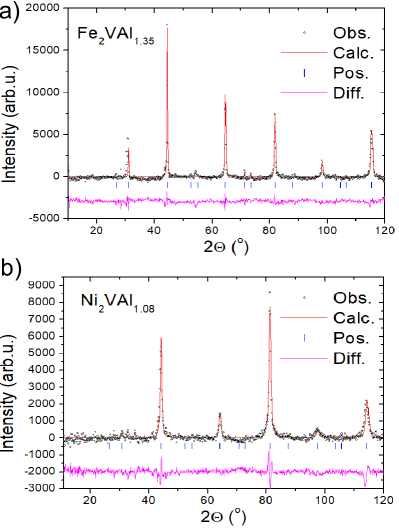
Figure 1: Plot of Rietveld refinement for Fe₂VAl_1.35 (a) and Ni₂VAl_1.08 (b). Black dots - observed pattern, red line - calculated, blue ticks - Bragg peaks positions, magenta line - the difference. The Ni₂VAl_1.08 alloy is extremely hard, so the stresses when preparing the sample for XRD analysis cause a greater spread of background intensities in the XRD diffraction pattern.

Table 1: Lattice parameters $a$ and stoichiometry.

compound	$a$ (Å)	composition (at%)
Fe2VAl1.35	5.7659(8)	$45.86:23.02:31.13$
Ni2VAl1.08	5.7996(9)	$49.48:24.25:26.27$
V2FeAl	5.9469(5)	$49.55:25.11:25.34$

Stoichiometry and homogeneity were checked using an electron energy dispersive spectroscopy (EDS) technique. The atomic percentage of the specific element content in Fe₂VAl, Ni₂VAl, and V₂FeAl is listed in Table 1. For Ni₂VAl, and V₂FeAl it deviates from the nominal composition $2:1:1$ at an acceptable level, while Fe₂VAl_1.35 was identified as off-stoichiometric with excess of Al and with a homogeneous distribution of atoms.

The ac magnetic susceptibility was measured in the temperature range 2-300 K with an ac field of 2 Oe and freqency from 100 Hz to 4 kHz using a Quantum Design PPMS platform. The dc magnetic measurementswere carried out in the temperature interval $1.7-400$ K and magnetic fields up to 7 T employing a Quantum Design superconducting quantum interference device (SQUID) magnetometer. Time-dependent remnant magnetization and high-temperature dc magnetic susceptibility ($300<T<800$ K) were measured using the PPMS platform equipped with a vibrating sample magnetometer (VSM) option. Electrical resistivity and heat capacity measuremments were performed in the temperature range $1.8-300$ K and in external magnetic fields up to 9 T using the same PPMS platform.

The x-ray photoelectron spectroscopy (XPS) spectra were obtained at room temperature with monochromatized Al $K_{\alpha}$ radiation using a PHI 5700/600 ESCA spectrometer. To obtain good quality XPS spectra, the samples were cleaved and measured in the vacuum of $6\times 10^{-10}$ Torr.

II.2 Computational methods

The electronic and magnetic properties of Fe₂VAl and Ni₂VAl, as well as the off-stoichiometry components, were theoretically studied using the ab initio, DFT-based full potential linearized augmented plane waves (FP-LAPW) method complemented with local orbitals (LO) [26]. The calculations were performed using the WIEN2k (ver. 19.1) package [27]. The atomic core states were treated within the fully relativistic DFT approach. For the local orbitals and valence states, (assumed as follows: V - [$3s^{2}3p^{6}$]_LO{$3d^{3}4s^{2}$}_VB; Fe - [$3s^{2}3p^{6}$]_LO{$3d^{6}4s^{2}$}_VB; Ni - [$3s^{2}3p^{6}$]_LO{$3d^{8}4s^{2}$}_VB and Al - [$2s^{2}2p^{6}$]_LO{$3s^{2}3p^{1}$}_VB) the scalar-relativistic Kohn-Sham formalism was applied with spin-orbit coupling (SOC) accounted for through the second variational method [26]. The generalized gradient approximation (GGA) for the exchange-correlation (XC) energy functional was applied in the form derived for solids by Perdew et al. (PBEsol) [28]. For the correlated $d$ states, the XC potential was corrected by on-site Hubbard-like interaction $U$ following the Anisimov at al. approach [29, 30]. In the calculations presented, we assumed the effective Hubbard parameter $U_{\rm eff}$ ($=U-J$) for $d$-states of Fe, Ni, and V we assumed equal to 3 eV.

For simulations of off-stoichiometric systems with antisite atoms, we employed the supercell spanned by doubled primitive vectors of the underlying L2₁ primitive cell, comprising eight formula units of Fe₂VAl (Ni₂VAl), based on which the superstructures were prepared with Al, Fe, Ni, and V atoms located at antisite positions. The calculations were performed for a basic Fe₂VAl and Ni₂VAl structures and superstructures with compositions: Fe₁₆(V₇Fe₁)Al₈, Fe₁₆(V₇Al₁)Al₈, Fe₁₆(V₅Al₃)Al₈, (Fe₁₅Al₁)V₈Al₈, (Fe₁₃Al₃)V₈Al₈, and Ni₁₆(V₇Ni₁)Al₈. Structural analysis revealed that the antisite atoms in the vanadium sublattice do not change the space group Fm$\bar{3}$m (no. 225) of the original Heusler structure, while those located in the Fe sublattice reduce the space group of the corresponding superstructure to the F4$\bar{3}$m (no. 216). Nevertheless, in all cases, the disorder caused by AS atoms, connected to the anisotropy introduced by the spin-orbit coupling, split the Wyckoff positions of the Heusler structure into several subgroups (see Table 3).

In the presented approach, the parameters decisive for the accuracy of the calculations employing the WIEN2k code, the number of $\vec{k}$ vectors in the Brillouin zone (BZ), and the plane wave cut-off energy ($K_{\rm max}$) were tested against the total energy convergence. A satisfactory energy precision of few meV for the base Fe₂VAl and Ni₂VAl was reached with $12\times 12\times 12$ k-mesh (163 $\vec{k}$ vectors in irreducible BZ) and $K_{\rm max}=9/R_{MT}$. The radii of the muffin-tin spheres $R_{MT}$ of 0.1058 nm were assumed as common for all atomic species. These settings were also adopted in the calculations for superstructures.

III Magnetic and transport properties in disordered Fe₂VAl_1.35 in reference to spin-fluctuator Ni₂VAl, experimental details and discussion

III.1 Magnetic properties

The magnetic and transport properties of Heusler alloys are highly dependent on stoichiometry, as well as the level of atomic disorder. Here we present the magnetic properties of Fe₂VAl_1+δ with excess of Al ($\delta\sim 0.35$) with respect to Ni₂VAl_1+δ ($\delta\sim 0.08$), we also discuss the impact of antisite defects on the localization of $3d$ electronic states of Fe and Ni in both alloys. A detailed analysis of the complex magnetic behaviors documented for Fe₂VAl_1+δ is also based on other thermodynamic and electron transport studies (in Sec. III.B-D), as well as ab initio electronic structure calculations, presented in Sec. IV.

Shown in Fig. 2 are the dc magnetic susceptibility $\chi$ data plotted as $\chi$ and $1/\chi$ vs. $T$ between 1.7 and 700 K for Fe₂VAl_1.35. The susceptibilities of Ni₂VAl_1.08 and V₂FeAl measured in the temperature region $T<300$ K are also displayed for comparison.

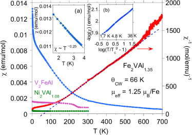
Figure 2: Temperature dependence of dc $\chi$ (blue points) and $1/\chi$ (red points) at 1000 G for Fe₂VAl_1.35. For comparison, the dc susceptibility $\chi(T)$ at 1000 G are shown for $V_{2}$FeAl (pink points) and for Ni₂VAl_1.08 (green points). Inset (a) shows the divergent behavior of $\chi$ for $T<4$ K, inset (b) presents $1/\chi$ vs. reduced $T$, $(T/T_{C}^{g}-1)$ in the log–log scale. We attribute the change in the susceptibility of Fe₂VAl_1.35 that occurs at $\sim 580$ K to a diffusion process that results in a more highly ordered sample above this temperature.

The $\chi^{-1}(T)$ follows a Curie law above $\sim 600$ K with the effective magnetic moment $\mu_{\rm eff}=1.26$ $\mu_{B}$ per one Fe atom in the formula unit. A very crude analysis predicts that statistically only one iron atom contributes to the value of $\mu_{\rm eff}$ per unit cell of Fe₂VAl_1+δ, assuming that only Fe ions contribute to the effective magnetic moment and $\mu_{\rm eff}$(Fe${}^{2+})=5.4$ $\mu_{B}$. Magnetization as well as the specific heat data suggest one order of magnitude smaller number of magnetic Fe defects in this system (will be discussed). DFT calculations confirm that this is an Fe ion in the antisite position, while the remaining Fe atoms in the surrounding of the AS defect are non-magnetic (will be discussed in Sec. IV). A Curie-Weiss (CW) law is obeyed in the range of $200<T<580$ K, indicating a peculiar magnetic state with random magnetic interactions below $\sim 200$ K and signaling the onset of weak ferromagnetism. The best fit to $\chi\sim(T-\theta_{CW})^{-1}$ gives the CW temperature $\theta_{CW}=66$ K and $\mu_{\rm eff}=1.25$ $\mu_{B}$ per Fe atom, i.e., almost four times smaller value of $\mu_{\rm eff}$ than that predicted for Fe²⁺. The magnetic susceptibility anomaly below 200 K has been found to arise from a distribution of magnetic defects in the sample (cf. Refs. [17]). Similar anomalous behaviors in $\chi$ appear to be characteristic of the family of Heusler alloys containing the magnetic transition metal $M$, regardless of the stoichiometry of the system (cf. $\chi(T)$ data for V₂FeAl in Fig. 2), while it is not present in almost paramagnetic Ni₂VAl_1.08. As an example, a well ordered V₂FeAl is expected to be a Pauli paramagnet [31, 32], while a weak magnetization below $\sim 230$ K can be induced in this material by wrong-site iron atoms as a result of incomplete structural ordering, as shown in Fig. 2. Our investigations suggest a similarity of this weakly magnetic state with short-range magnetic correlations with the behavior of the Griffiths phase (GP) scenario [18]. The distinct similarities to the Griffiths phase have already been suggested earlier for the off-stoichiometric Fe₂VAl [9], as well as for the (FeNi)TiSn alloy [33] and disordered Fe₂VAl [34] due to the presence of AS defects.

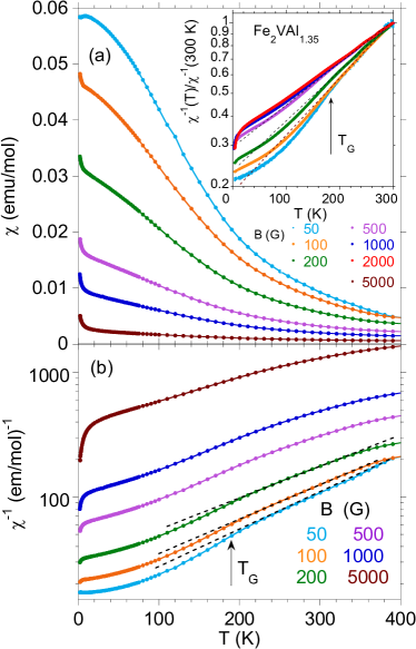
Figure 3: (a) Susceptibility and (b) inverse susceptibility (in log scale) vs temperature data from QD SQUID magnetometer, measured for Fe₂VAl_1.35 in different values of applied fields. The inset shows similar data of $\chi(T)^{-1}$ normalized to $1/\chi$ at 300 K (in log scale) obtained from a commercial QD PPMS-VSM platform. The dashed lines approximate the CW behavior to low temperatures to show the downward effect in $\chi^{-1}$ below temperature $T_{G}\sim 200$ K.

The Griffiths phase consists of magnetic clusters in a paramagnetic phase much above $T_{C}$ and forms as a result of the competition between the Kondo effect and the Ruderman-Kittel-Kasuya-Yosida (RKKY) interaction in the presence of disorder [18]. Namely, in the temperature region $T_{C}^{g}<T<T_{G}$, where $T_{G}$ is a Griffiths temperature, the system is considered to exist in the GP that exhibits neither pure paramagnetic behavior nor long-range ferromagnetic (FM) order. In this framework, the Griffiths phase is a peculiar state that is predicted to occur in randomly diluted Ising FM systems [35, 36], in which magnetization fails to become an analytic function of the magnetic field over a temperature range $T_{C}^{g}<T<T_{G}$. Usually, Griffiths singularity is signed by a nonlinear variation of the inverse magnetic susceptibility in the paramagnetic phase [37], namely $\chi^{-1}\propto(T-T_{C}^{g})^{(1-\lambda)}$ ($0<\lambda<1$) [38, 39], where $T_{C}^{g}$ is the critical temperature of random ferromagnetism of the sample where susceptibility tends to diverge. According to the $\chi$-data shown in Fig. 2, the deviation from the CW law is evidenced for $T<200$ K, while below $T=4$ K the dc susceptibility exhibits a power-law behavior, $\chi\sim T^{-n}$, with exponent $n=1-\lambda=0.25$ [38]. Moreover, for $1.7<T<40$ K $\chi$ can be well characterized by expression $\chi(T)\sim(T-T_{C}^{g})^{-(1-\lambda)}$ with the fitting parameters $T_{C}^{g}=1.3$ K and $\lambda=0.7$.

According to the GF scenario, $\chi$ shown in Fig. 2 deviates from the CW law below $T\equiv T_{G}=200$ K, while for $T<4$ K susceptibility exhibits a power-law behavior, $\chi\sim T^{-n}$, with exponent $n=1-\lambda=0.25$ [38]. Moreover, for $1.7<T<40$ K $\chi$ can be well characterized by expression $\chi(T)\sim(T-T_{C}^{g})^{-(1-\lambda)}$ with the fitting parameters $T_{C}^{g}=1.3$ K and $\lambda=0.7$. Fig. 3 shows the $\chi(T)$ dc data measured at various magnetic fields $50<B<5000$ G. In the field of 50 G $\chi$ exhibits a maximum at $\sim 9$ K indicative of a magnetic glassy behavior, while $\chi$ measured at larger fields shows divergent behavior at the lowest temperatures. The inset to Fig. 3 presents the inverse susceptibility divided by the value of $\chi^{-1}$ at 300 K in different fields as a function of $T$ from the VSM experiment, to show more details. For $T>200$ K $\chi^{-1}$ varies linearly with $T$, following the CW behavior. However, with the decrease in $T$, a clear downturn in $\chi^{-1}$ is observed at $T\approx 200$ K (much above $T_{C}^{g}$) for the measurements performed in dc fields $B\leq 500$ G, indicating non-analytic behavior of $M$ arising from the Griffiths singularity. The softening of the downward behavior in $\chi^{-1}$ and the progressive increase of $\chi^{-1}$ in the field (cf. Fig. 3) are characteristic properties of the GP state (cf. [39]), both allowed to distinguish the Griffiths singularity from smeared phase transition between the paramagnetic and ferromagnetic states.

We also comment on the field-induced divergence of the value of $\chi$, shown for Fe₂VAl_1.35 in Fig. 3. This field-dependent $\chi(T)$ plots may result from a trace amount of magnetic Fe impurities, can be caused by spin fluctuations quenched by the field (cf. [40, 41]), and/or may be caused by the various size of clusters field-dependent. For the first scenario, the appearance of Fe impurities should cause an increase in $\chi$ with an increasing field; this is not a case. The effect of spin fluctuations on the value of $\chi$ seems to be possible for Fe₂VAl_1.35 since similar field-induced $\chi(T)$ behavior has also been observed for spin-fluctuator Ni₂VAl. Note that spin fluctuation gives a dominant effect around $T_{C}$, but is also important much above $T_{C}$, since the energy scale of spin fluctuations is usually two orders of magnitude larger than $T_{C}$ for itinerant electron ferromagnets [42, 43]. The magnetic properties shown in Fig. 3 are more likely the result of contributions from both fluctuating moments and cluster size effects, as has been reported for a variety of nanoparticles (e.g., Refs. [44, 45, 46]).

The ac magnetic susceptibility was measured at various frequencies in order to confirm the hypothesis of spin/cluster-glass state in Fe₂VAl_1.35. Shown in Fig. 4 are the real ($\chi^{\prime}$) and imaginary ($\chi^{\prime\prime}$) components of the magnetic ac susceptibility data. $\chi^{\prime}$ [in panel (b)] and $\chi^{\prime\prime}$ [in panel (c)] exhibit a broad maxima at $\sim 15$ K with amplitudes and positions depending on the frequency $\nu$ of the applied magnetic field. The maximum of $\chi^{\prime}$ can be attributed to a spin-glass-like transition, which is commonly used to determine the spin freezing temperature $T_{f}$. The frequency dependence of $T_{f}$ follows the empirical Vogel-Fulcher relation that is described as $\nu=\nu_{0}\exp[-E_{a}/k_{B}(T_{f}-T_{0})]$, where $\nu_{0}$, $T_{0}$, and $E_{a}$ are fitting parameters [47]. Taking into account the microscopic single spin flipping frequency $\nu_{0}\sim 10^{13}$ Hz for spin–glass materials we obtained $E_{a}=290$ K and $T_{0}=1.7$ K, fitting this expression to the linear change of $T_{f}$ versus $1/\ln(\nu_{0}/\nu)$. The parameter $T_{0}$ does not have a precise physical meaning; it is proposed to be related to the true critical temperature when $T_{f}>T_{0}$ is only a dynamic manifestation of the magnetic transition from paramagnetic to SG phase, cf. Ref. [47]. The frequency shifts of the $\chi^{\prime}$ maxima yield ratio $\delta T_{f}=\Delta T_{f}/T_{f}\Delta\log_{10}\nu\approx 0.02$, which is one order of magnitude higher than expected for canonical metallic spin-glass materials ($\sim 10^{-3}$), but fits well with the range that is reported for cluster-glasses [47].

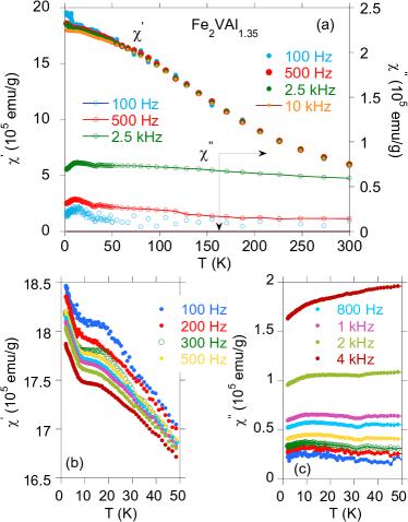
Figure 4: Temperature dependence of the real and imaginary part of the ac magnetic susceptibility $\chi_{ac}$ for Fe₂VAl_1.35 measured for various frequencies of the applied magnetic field; the amplitude of the magnetic field was 2 G. Panels (b) and (c) show details over a limited temperature range for $T<50$ K. Panel (b) shows the obvious step-like changes in $\chi^{\prime}$ at about 20 K, 30 K, and 40 K, which are magnified for clarity in Fig. 5.

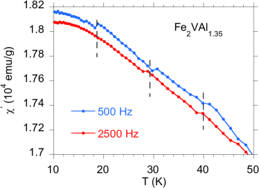
Figure 5: Magnetic susceptibility $\chi^{\prime}$ as a function of temperature; drops in $M^{\prime}$ during stops at 19, 30 and 41 K are magnified for clarity (cf. Fig. 4) and will be discussed in Sec. III.B.

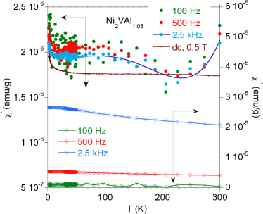
Figure 6: Temperature dependence of the real and imaginary part of the ac magnetic susceptibility $\chi_{ac}$ for Ni₂VAl_1.05 measured for various frequencies of the applied magnetic field; the amplitude of the magnetic field was 2 G. Comparison with dc magnetic susceptibility measured for Ni₂VAl_1.05 in the field 5000 G.

Fig. 6 shows quite different behavior in $\chi_{ac}(T)$ for Ni₂VAl_1.08, namely, a broad maximum in $\chi^{\prime}$ is observed at about 100 K, which is indicative of the spin fluctuations.

We have studied the isothermal magnetic relaxation phenomenon in Fe₂VAl_1.35 and Ni₂VAl_1.08 as a final test of glassy state formation in these alloys. The samples were first zero field cooled from 300 K down to 8 K with a constant cooling rate and kept at a target temperature for a waiting time $t_{w}=300$ s in the field of 5000 G. Then the field was switched off. Figure 7 displays the time evolution of magnetization $M$ measured in zero-field-cooled (ZFC) mode at temperature 8 K for an applied field of 0.04 G. Various functional forms have been proposed to describe magnetization as a function of observation time [47]. The time dependence of $M$ shown in Fig. 7 for Fe₂VAl_1.35 is well approximated by the expression for magnetic viscosity $M(t)=M(0)+S\ln(1+t/t_{0})$, where $M(0)$ is the magnetization at $t=0$, $t_{0}=375$ s is the reference time, and $S=2.3\times 10^{-4}$ emu/g is the magnetic viscosity. The reference time $t_{0}$ is typically orders of magnitude larger than the observed microscopic spin flip $\tau_{0}$. The estimated values of $S$ are comparable to the results reported for other glassy systems. The magnitude of $M(t)$ strongly depends on $t_{w}$ before switching on the field [47]. However, this behavior is out of the scope of this research. Alternatively, $M(t)$ can be well approximated by an expression $M(t)=M_{0}+M_{r}\exp[-(t/\tau_{r})^{1-n}]$, where magnetization $M(0)=0.0092$ emu/g could be interpreted as an intrinsic weakly ferromagnetic component that appears below $\sim 200$ K in effect of sample disorder (cf. Fig. 2), while $M_{r}=0.0031$ emu/g could be related to a glassy component that mainly contributes to the relaxation effects observed. Within the disordered scenario, the magnetic clusters of Fe are distributed in the weakly magnetic background. In this approximation, the time constant $\tau_{r}=1.8\times 10^{5}$ s and the parameter $n=0.35$ [48] are related to the relaxation rate of the spin-glass-like phase [49].

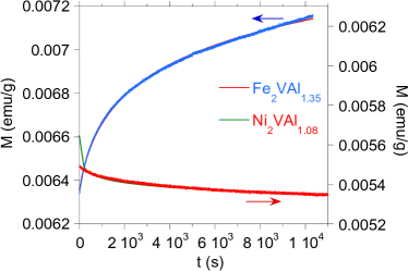
Figure 7: Time dependent remnant magnetization behavior for Fe₂VAl_1.35 (blue points) and Ni₂VAl_1.08 (red points). The red solid line represents a fit to equation $M(t)=M(0)+S\ln(1+t/t_{0})$, the green solid line represents the best fit to equation $M(t)=M(0)t^{-\alpha}$.

Figure 7 compares a similar isothermal remnant magnetization (IRM) as a function of time, measured for Ni₂VAl_1.08 at 8 K under the same conditions. The observed time dependence of IRM is weakly $t$-dependent and can be fitted by the power-law decay, $M(t)=M(0)t^{-\alpha}$ with the fitting parameter $\alpha=6.2\times 10^{-3}$, however, only for $t>200$ s. Below this time limit, the $M(t)$ data do not follow the $M(0)t^{-\alpha}$ behavior. The $M(t)$ dependence shown for Ni₂VAl_1.08 in Fig. 7 signals the presence of diluted and disordered magnetic moments of AS Ni defects (will be discussed) which, however, do not form an ordered glassy state.

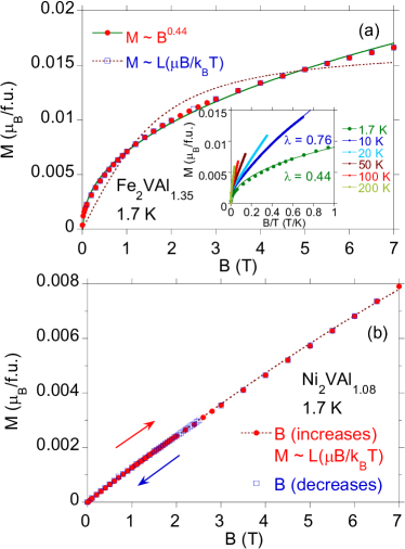
Figure 8: Isothermal magnetization as a function of applied magnetic field of Fe₂VAl_1.35 (a) and Ni₂VAl_1.08 (b) for 1.7 K. The red dotted line is a fit of the Langevin function $L$ to the magnetization data. In panel (a) the green line shows the approximation of the expression $M=M(0)+mB^{\lambda}$ to the experimental data. The inset displays $M$ vs $B/T$; in this plot the $M$ isotherms are approximated by the $M\sim B^{\lambda}$ expression for $T=1.7$ K and 10 K, respectively.

To further probe the nature of the magnetic ground state in Fe₂VAl_1.35 and Ni₂VAl_1.08 Heusler alloys, the isothermal magnetization $M$ was measured as a function of magnetic field, as shown in Fig. 8. The $M(B)$ isotherms of Fe₂VAl_1.35 do not exhibit any hysteresis loop, however, are also not characteristic of paramagnets. The $M(B)$ characteristics cannot be approximated by the Langevin function $L(\xi)=\coth(\xi)-1/\xi$ ($\xi=\mu B/k_{B}T$ and $\mu$ is the total magnetic moment), as shown in panel (a). Moreover, $M$ is not a universal function of $B/T$ as displayed in the inset to Fig. 8(a). This scaling behavior is characteristic of the superparamagnetic state, which is not the case. Whereas, magnetization as a function of the field up to 7 T follows the predicted Griffiths phase behavior $M\sim B^{\lambda}$ [50], as shown in Fig. 8(a). Within the Griffiths phase scenario the $M\sim B^{\lambda}$ well approximates the experimental data and gives $\lambda=0.76$ for the $M(B)$ data at $T=10$ K. The fitting procedure of $M$ at $T=1.7$ K gives $\lambda\sim 0.45$ smaller than expected, the reason is due to the increase of magnetic correlations for $T\rightarrow T_{C}^{g}$ that lead to a glassy state and dominate the Griffiths phase state. Figure 8(b) displays the paramagnetic $M$ vs. $B$ behavior for Ni₂VAl_1.08 at 1.7 K, well approximated by the Langevin function $L(\xi)$.

Finally, we present some notes on the magnetic ground state in the disordered Fe alloy. While the parent compound Fe₂VAl has a nonmagnetic ground state, its disordered analogues determined by the presence of vacancies at various crystallographic sites, off-stoichiometry, and/or doping are very close to ferromagnetic ordering, as has been demonstrated by many studies (cf. Ref. [41] and references therein). The divergence in the $\chi(T)$ data shown in Fig. 2 suggests this possibility at the limit of $T\rightarrow 0$.

III.2 Memory effect in Fe₂VAl_1.35

The non-zero value of $M(0)$ in Fig. 7 indicates the coexistence of weakly magnetic and glassy magnetic components in the relaxation process. It can be assumed that the small clusters of Fe are separated in the weakly magnetic phase. The phase separation scenario would be favorable to explain the existence of out-of-equilibrium features shown in $\chi^{\prime}(T)$ data in Figs. 4 and 5, as competition between coexisting phases, leading to the appearance of locally metastable states observed in ac susceptibility, as memory effect in the cooling cycle. In our ac magnetization measurements, a field with an amplitude of 2 G was applied during cooling. An analogous behavior was observed for Fe-doped phase separated manganite La_0.5Ca_0.5MnO₃ [51] and for Dy_0.5Sr_0.5MnO₃ [52].

III.3 Specific heat

Fig. 9 compares the temperature dependence of the specific heat for Fe₂VAl_1.35 and of Ni₂VAl_1.08, measured in a zero magnetic field. For both alloys, the value of $C$ per one atom reaches the value of $3R$ in accordance with the Dulong-Petit law ($R$ is the gas constant). The $C(T)$ data are well approximated by the Debye-Einstein (DE) model [53]:

$$C(T) = \gamma_{0}T+9NR(1-d)\left(\frac{T}{\Theta_{\rm D}}\right)^{3}\int_{0}^{\Theta_{\rm D}/T}\frac{x^{4}\;e^{x}}{(e^{x}-1)^{2}}dx$$ (1)

$$+\>3nRd\left(\frac{\theta_{E}}{T}\right)^{2}\frac{e^{\theta_{E}/T}}{(e^{\theta_{E}/T-1})^{2}},$$

where the first term is the electron specific heat $C_{el}(T)=\gamma_{0}T$, and the two others account for the lattice contributions ($\theta_{D}$ and $\theta_{E}$ are the Debye and Einstein temperatures, respectively, $n$ is the number of atoms per formula unit, and $d$ stands for the number of optical phonon modes).

The solid lines show temperature variation of the calculated $C(T)$ with the fitting parameters $\gamma_{0}=33$ mJ/molK², $\theta_{D}=638$ K, $\theta_{E}=297$ K, and $d=0.51$ for Fe₂VAl_1.35, and respective set of the fitting parameters for Ni₂VAl_1.08 ($\gamma_{0}=11$ mJ/molK², $\theta_{D}=492$ K, $\theta_{E}=148$ K, and $d=0.69$). Equation (1) does not take into account the magnetic contributions from the spin glass state, therefore, at the temperatures $T<20$ K the fitting is not satisfactory for Fe₂VAl_1.35, which is the reason for the overestimated value of $\gamma_{0}$.

The $\gamma_{0}$ and $\beta_{0}$ derived from the linear sections (for $T>6$ K) of $C/T$ vs $T^{2}$ dependence are 5.5 mJ/K² mol and $4.6\times 10^{-5}$ J/K⁴ mol, respectively, indicating the pseudogap in the bands of Fe₂VAl_1.35 at the Fermi level. The $\gamma_{0}$ and $\beta_{0}$ determined similarly for Ni₂VAl_1.08 in the temperature range $T<15$ K are respectively, 13.5 mJ/K² mol and 2.6 J/K⁴ mol. Moreover, these fitting parameters obtained from the approximation of Eq. (1) to $C(T)$ as well those from linear dependence of $C/T$ vs. $T^{2}$ are similar.

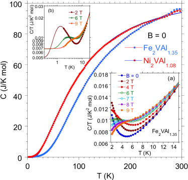
Figure 9: Specific heat for Fe₂VAl_1.35 (blue points) and Ni₂VAl_1.08 (red points) measured in a wide temperature range and a fit of Eq. (1) to the experimental data. In panel (a), the temperature dependence of $C/T$ in various magnetic fields. The continuous curves are the fits of a two-level Schottky-like function $C_{\rm Sch}$, lattice $\beta T^{3}$, and electronic $\gamma T$ contributions to the $C/T$ data (cf. Table 2). The inset (b) shows in detail the approximation of the two-level Schottky function to the experimental data $C/T$ for Fe in the field of 2, 6, and 9 T.

For $N=4$ atoms in formula unit, $\beta=N(12/5)\pi^{4}R\theta_{D}^{-3}$ gives the Debye temperature, $\theta_{D}\sim 567$ K for Fe₂VAl_1.35 and $\theta_{D}\sim 304$ K for Ni₂VAl_1.08, respectively. In both cases, the determined temperatures $\theta_{D}$ are close to those obtained by fitting the DE function [Eq. (1)] to the $C(T)$ data.

Inset (b) displays the low-temperature specific heat $C$ divided by temperature, $C(T)/T$, at various magnetic fields for Fe₂VAl_1.35. The upturn in $C/T$ at $B\neq 0$ can be interpreted as a result of Schottky-like anomalies due to magnetic defects [54, 55]. Assuming that the specific heat is a sum, $C_{\rm magn}+\gamma T+\beta T^{3}$, the $C/T$ data at various magnetic fields are well approximated to expression $C/T=C_{\rm Sch}/T+\gamma+\beta T^{2}$, where $C_{\rm Sch}$ is a two-level Schottky function

$$C_{\rm Sch}=N_{Fe}k_{B}\left(\dfrac{\epsilon}{T}\right)^{2}\dfrac{e^{\epsilon/T}}{(1+e^{\epsilon/T})^{2}},$$ (2)

with $\epsilon$, $\gamma$, and $\beta$ field dependent (cf. Table 2). In the inset (b) to Fig. 9 the solid lines are the best fits of $C_{\rm Sch}/T+\gamma+\beta T^{2}$ to the $C/T$ experimental data of Fe₂VAl_1.35. A simple fit of the Schottky function to $C(T,B=0)$ data gives $\sim 10\times 10^{19}$ cm^-3 of Schottky centers $N_{Fe}$. Assuming that Fe_AS defects dominate in the sample, and taking $g=1.93$ and $S=3/2$ for the antisite defects, the saturation magnetization of Fe₂VAl_1.35 (cf. Fig. 8$a$) expressed by $M_{S}=N_{Fe}g\mu_{B}S$ gives comparable magnetic impurity concentration of $\sim 13\times 10^{19}$ cm^-3 which, when calculated per unit cell, gives about 0.02 atom per cell in the antisite position. One also notes that the $\epsilon$ vs. $B$ change is well approximated by expression $\epsilon(B)=\epsilon(0)+bB^{n}$ with exponent $n=1.6$, moreover, in the constant field mode, each value of $\epsilon/k_{B}$ is obtained twice larger than the value of $T\equiv T_{f}$ at which $C_{B={\rm const}}(T)/T$ has the maximum.

Table 2: Specific heat $C(T)$ parametrization of Fe₂VAl_1.35 within temperatures $T<15$ K. $C(T)$ is fitted to the two-level Schottky function supplemented with electron ($\gamma T$) and phonon ($\beta T^{3}$) contributions. Comparison with electronic specific heat coefficients $\gamma_{0}$ and coefficients $\beta_{0}$ experimentally obtained from a least-squares fit of expression $C(T)/T=\gamma_{0}+\beta_{0}T^{2}$ to the experimental data in the temperature region between $\sim 5$ K and $15$ K (cf. Fig. 10).

		$C=N_{Fe}k_{B}(\epsilon/T)^{2}e^{\epsilon/T}/(1+e^{\epsilon/T})^{2}+\gamma T+\beta T^{3}$		$C=\gamma_{0}T+\beta_{0}T^{3}$
$B$ (T)	$\epsilon$ (K)	$\gamma$ (mJ/K2 mol)	$\beta\times 10^{5}$ (J/K4 mol)	$\gamma_{0}$ (mJ/K2 mol)	$\beta_{0}\times 10^{5}$ (J/K4 mol)
0	2	4.7	5.0	5.5	4.6
2	3.2	4.9	4.8	6.0	4.4
4	4.7	5.7	4.5	6.9	4.0
6	6.2	6.7	4.1	7.7	3.8
7	7.5	7.0	4.8	8.0	3.6
8	9.0	7.1	4.0	8.3	3.6
9	10.8	6.8	4.2	8.5	3.5

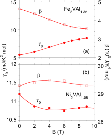
Figure 10: Electronic specific heat coefficient $\gamma_{0}$ and coefficient $\beta$ vs applied magnetic field $B$. $\gamma_{0}$ and $\beta$ are obtained from the linear dependence of $C(T)/T=\gamma_{0}+\beta T^{3}$ vs. $T^{2}$ for Fe₂VAl_1.35 and for Ni₂VAl_1.08 in the temperature region between $\sim 5$ K and $15$ K.

Figure 10 shows the electronic specific-heat constant $\gamma_{0}$ and the coefficient of the $T^{3}$ term $\beta$ for Fe and Ni samples as a function of the magnetic field. It is worth noting that the field dependencies either of $\gamma_{0}$ and $\beta$ are for Ni₂VAl_1.08 typical for systems with spin fluctuations. Namely, the field-induced behavior of $\gamma_{0}$ and $\beta$ shown in panel (b) as well as $\chi(T)$ shown in Fig. 6 are similar to those, observed for canonical spin fluctuator CeSn₃, which was classified by Ikeda et al. [56] as a type 3 spin fluctuator.

Fe₂VAl_1.35 exhibits significantly different corresponding characteristics, as shown in panel (a). An increase in $\gamma_{0}$ shown in Fig. 10 we attribute to a strong reducing of the pseudogap at the Fermi level by increasing the field, which consequently gives an increase of $\gamma$. Our previous research of similar Heusler alloys (Fe₂TiSn [17], Fe₂VSn [57]) explicitly documented that the physical properties of these semiconductors, in particular resistivity, susceptibility, and specific heat are dominated by crystallographic disorder. The AS atomic disorder can generate the narrow $d$-electronic band located at the Fermi level, which is responsible for the unusual temperature dependencies (these materials can also be discussed as false Kondo insulators).

Figure 11 shows entropy $S$ for Fe₂VAl_1.35 and Ni₂VAl_1.08 in the temperature region $T<100$ K. Assuming that only conduction electrons, phonons and spin fluctuations contribute to $S$, then the entropy of Ni₂VAl_1.08 can be well fitted by expression [58]:

$$S=\int_{0}^{T}\frac{dC}{T} = \int_{0}^{T}\frac{\gamma_{0}T+\beta T^{3}+\delta T^{3}\ln(T/T^{\star})}{T}dT$$ (3)

$$= \gamma_{0}T+\frac{\beta}{3}T^{3}+\frac{\delta}{3}T^{3}\ln\frac{T}{T^{\star}}-\frac{\delta}{9}T^{3},\hskip 17.07164pt$$

where $T^{\star}=120$ K, $\gamma_{0}=13$ mJ/K² mol, $\beta=1.5\times 10^{-4}$ J/K² mol, and $\delta=-1.7\times 10^{-4}$ J/K⁴ mol (cf. Fig. 11). The fit is very good for $T>30$ K, but for lower temperatures this approximation deviates from the experimental data, even within 10% around 15–20 K. A possible reason for this divergence may be the Kondo effect due to scattering of conduction electrons on magnetic Ni impurities, which can give an additional contribution to $S$ (in Sec. IV we will document in ab initio calculations that Ni at AS positions has a localized magnetic moment) . Figure 12 presents low-temperature $C/T$ vs. $T^{2}$ data at various fields for Ni₂VAl_1.08, with an obvious and field-dependent upturn in $C/T$ for $T^{2}<40$ K. This behavior is not typical of spin fluctuators for which the quenching of the magnetic contribution to the heat capacity by the magnetic field is usually detected. The possible explanation for the low-temperature heat capacity enhancement shown in Fig. 12 can be the formation of a Kondo resonance. Indeed, the heat capacity $C/T$ measured in varying magnetic fields shows typical behavior of diluted Kondo systems [59, 60], and well correlates with the low-$T$ resistivity data (see Sec. III.C).

Expression (3), however, does not fit well the $S$ data of Fe₂VAl_1.35. In this case, the entropy shows a kink at $T\sim 3$ K due to freezing of the glassy phase (see the inset to Fig. 11), and can be well approximated by expression $S(T)\sim\gamma_{0}T+\beta T^{3}+sT^{n}$ with exponent $n=3/2$ for $T<3$ K and $n=-2$ for $T>3$ K [61], respectively, as shown in Fig. 11 (for both cases, $\gamma_{0}=5.5$ mJ/K⁴ mol, $\beta=1.9\times 10^{-4}$ mJ/$K^{4}$ mol).

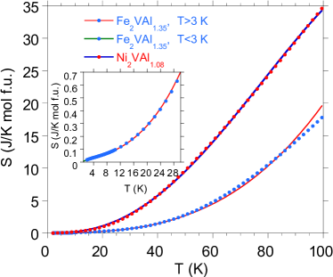
Figure 11: Ni₂VAl_1.08, the fit of Eq. (3) to entropy $S$ (blue line). For Fe₂VAl_1.35 entropy is well approximated by expression $S(T)\sim\gamma_{0}T+\beta T^{3}+sT^{n}$ with exponent $n=3/2$ for $T<3$ K (green line) and $n=-2$ for $T>3$ K (red line). The inset displays details.

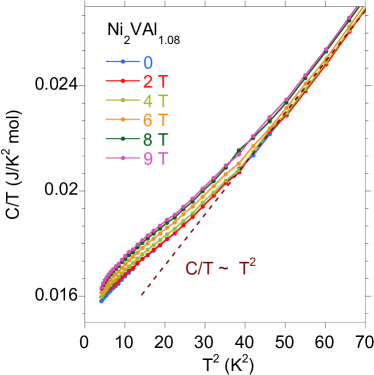
Figure 12: Heat capacity $C/T$ vs $T^{2}$ for Ni₂VAl_1.08 in magnetic fields. The linear $C/T$ vs $T^{2}$ behavior is obeyed for temperatures $6<T<20$ K.

III.4 Electron transport properties

Previous reports have indicated that even a small deviation in the stoichiometry of Fe₂VAl has a significant impact on its electron transport properties [15]. Similarly, the thermal heat treatment of this alloy has a decisive impact on its electric and thermal transport [62]. So far, electron transport investigations were focused on the Fe₂VAl alloys with a deficiency of both Fe, V and Al, mainly in terms of enhancing the thermoelectric properties. The aim of the current research was to demonstrate to what extent an excess of Al can change the thermoelectric properties of Fe₂VAl. However, our research did not confirm the expectations of significant strengthening of the thermoelectric properties of this alloy. The results obtained for Fe₂VAl_1+δ were compared with electron transport measurements for Ni₂VAl.

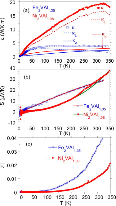
Figure 13: Temperature variation of thermal conductivity $\kappa$ (a), Seebeck coefficient $S$ (b), and figure of merit $ZT$ (c) of Fe₂VAl_1.35 (blue open squares) and for Ni₂VAl_1.08 (red points). Panel (a) also shows lattice (dotted line) and electronic (solid line) thermal conductivitiy for Fe₂VAl_1.35 (blue) and Ni₂VAl_1.08 (red), respectively. Panel (b) shows the fit of the SF model (Eq. 4) to the $S(T)$ data for Fe₂VAl_1.35 (red solid line) and Ni₂VAl_1.08 (blue solid line). The experimental data of Ni₂VAl_1.08 deviate from the fit around $\sim 270$ K (broad maximum).

Figure 13 compares the thermal conductivity $\kappa$, Siebeck coefficient $S$, and figure of merit $ZT$ of Fe₂VAl_1.35 and Ni₂VAl_1.08. Panel (a) shows $\kappa$, which is a sum of electronic ($\kappa_{e}$) and lattice ($\kappa_{L}$) contributions, measured between 2 and 350 K. In general, metals with higher Debye temperatures tend to have higher thermal conductivities. Therefore, one could expect a higher thermal conductivity for Fe₂VAl_1.35 than for its Ni₂VAl_1.08 analogue. Fe₂VAl_1.35 seems to be, however, an exception to this rule due to the presence of the pseudogap formed at the Fermi level due to interband hybridization, sample off-stoichiometry, and larger concentration of its antisite defects, all of which contribute to lowering the thermal conductivity of Fe₂VAl_1.35 in respect to $\kappa$ of metallic Ni₂VAl sample.

The electronic thermal conductivity was evaluated using the Wiedemann-Franz law: $\kappa_{e}\rho/T=L_{0}$, where $\rho$ is the measured dc electrical resistivity and $L_{0}=2.45\times 10^{-8}$ W$\Omega$K^-2 is the Lorenz number, while $\kappa_{L}$ was obtained by subtracting $\kappa_{e}$ from the measured $\kappa$. The temperature dependencies of $\kappa_{L}$ and $\kappa_{e}$ shown in Fig. 13(a) are typical of disordered crystalline materials where phonon scattering by defects and grain boundaries dominates.

As shown in Fig. 13(b), Seebeck coefficient $S$ obtained for Ni₂VAl_1.08 is approximated by Eq. 4, which expresses the temperature dependence of $S_{SF}(T)$ for nearly ferromagnetic, spin fluctuating metals [63] such as YCo₂ [64], under the condition that their susceptibility $\chi(T)$ shows a broad maximum (cf. Fig. 6),

$$S_{SF}=\tilde{\alpha}T+\tilde{\beta}T\left(\frac{T}{\tilde{T}_{0}}\right)\log\frac{\tilde{\delta}+(T/\tilde{T}_{0})^{2}}{(T/\tilde{T}_{0})^{2}}.\hskip 17.07164pt$$ (4)

Within this modeling, $d$ electrons are responsible for the spin fluctuation, while transport properties are due to conduction electrons, which are dragged by spin fluctuations (SF), $\tilde{\alpha}$, $\tilde{\beta}$, $\tilde{\delta}$, and $\tilde{T}_{0}$ are fitting parameters. The fitting procedure gives $\tilde{\alpha}=0.029$ $\mu$V K^-2, $\tilde{\beta}=0.053$ $\mu$V K^-2, $\tilde{T}_{0}=220$ K, and $\tilde{\delta}=4.3$ for Ni₂VAl_1.08. The experimental data for $S(T)$ of Fe₂VAl_1.35 can also be approximated by expression (4) with the fitting parameters $\tilde{\alpha}=0.108$ $\mu$V K^-2, $\tilde{\beta}=-0.021$ $\mu$V K^-2, $\tilde{T}_{0}=300$ K, and $\tilde{\delta}=4$. Nonetheless, spin fluctuations do not significantly enhance the value of figure of merit, $ZT$, which for the both alloys is about $10^{-2}$ at 350 K, as shown in Fig. 13(c).

In Fig. 14 we present the resistivity $\rho$ of Fe₂VAl_1.35 at different magnetic fields. The $\rho(T)$ data deviates from those, usually reported for stoichiometric Fe₂VAl compound [40, 65] and exhibit a semiconducting-like behavior, similar to that, reported for Fe₂TiSn [66, 67] and its alloys [57].

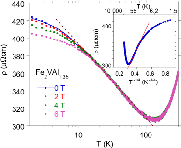
Figure 14: Resistivity vs. temperature (ln$T$ scale) of Fe₂VAl_1.35 in magnetic fields up to 6 T. The dashed line indicates the ln$T$ behavior in $\rho(T)$. The expression $\rho(T)=\rho_{0}+bT^{5}+c\ln(\mu/T)+\rho_{vrh}\exp(T_{0}/T)^{1/4}+r_{SG}T^{3/2}$ fits the $\rho(T,B=0)$ data between 2 and 100 K (blue line), where the respective parts are the phonon, Kondo, Mott-VRH, and spin-glass contributions to the resistivity. The inset shows $\ln\rho$ vs. $T^{-1/4}$, with the linear change of $\rho$ marked by the red line.

Between $\sim 100$ and 10 K $\rho\sim-lnT$, which is usually characteristic of Kondo behavior, whereas a significant deviation from linearity is observed below 10 K. However, we note that within this low-$T$ range there is observed a complex glassy-like phase, which complicates the interpretation of the $\rho$-data. Moreover, for $30<T<100$ K conductivity follows $\sigma=\sigma_{vrh}\exp[-(T_{0}/T)^{1/4}]$ (see Fig. 14, inset), which is typical for Mott variable-range hopping (VRH) behavior in three dimensions [68, 69]. Here $T_{0}$ characterizes the pseudogap at the Fermi level in the case of solids, where a conduction and valence band overlap giving a finite density of states $DOS(\epsilon_{F})$ (see Sec. IV). With increasing overlap of the bands, mostly the $d$-electron states become delocalized, which can lead to a metal-insulator transition of Anderson type. In the limit of weak localization, conduction by hopping (VRH) could be possible, this is a case of the Fe sample. $T_{0}$ inversely depends on the localization length $\xi_{L}=[\frac{1}{18}DOS(\epsilon_{F})k_{B}T_{0}]^{-1/3}$, which diverges at the insulator-metal transition [70]. The best approximation of $\rho=\rho_{vrh}\exp[(T_{0}/T)^{1/4}]$ to the experimental data shown in Fig. 14 gives $\rho_{vrh}=208.7$ $\mu\Omega$cm and $T_{0}=2.3$ K. Then, the localization length $\xi_{L}\approx 260$ Å for $DOS(\epsilon_{F})=1.078$ states/eV (cf. Table 3) is quite large, indicating direct proximity to the insulator-metal transition. Due to the above, we suggest that the hopping between Anderson-localized states is possible. Very recently, a similar conclusion was presented for stoichiometric Fe₂VAl [62].

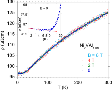
Figure 15: Resistivity of Ni₂VAl_1.08 vs temperature in applied magnetic fields. In applied magnetic fields $\rho$ vs $T$ is measured with chaotic distribution of the experimental points with respect to the curvature of $\rho(T)$ for zero field. This chaotic spread of experimental points increases with increasing $B$. The inset shows a Kondo impurity behavior $\rho\sim-lnT$.

The electrical transport of Fe₂VAl_1.35 reflects its complex interband and magnetic interactions; therefore, the resistivity of this alloy is discussed in relation to the paramagnetic Ni₂VAl_1.08. Figure 15 displays the resistivity of Ni₂VAl_1.08 as a function of temperature and in various magnetic fields. The $\rho(T)$ shown in the figure is almost not field-dependent. What is interesting, at the lowest temperatures $\rho\sim-\ln T$, suggesting the scattering mechanism of conduction electrons due to the presence of magnetic Ni impurities (Kondo impurity effect).

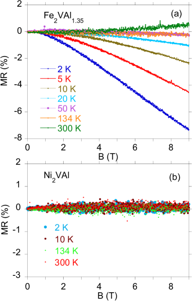
Figure 16: (a) Magnetoresistance $MR=[\rho(B)-\rho(B=0)]/\rho(B=0)\times 100$% ($I=5$ mA), of Fe₂VAl_1.35 (a) and Ni₂VAl_1.08 (b) as a function of the magnetic field $B$, measured at several temperatures.

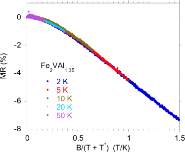
Figure 17: Schlottmann-type plot of the magnetoresistance isotherms from panel Fig. 16(a). $T^{\star}=2.9$ K.

Figure 16 compares magnetoresistance isotherms, $MR$, of Fe₂VAl_1.35 (a) and Ni₂VAl_1.08 (b) measured from $0-9$ T. $MR$ is defined as $MR=[\rho(B)-\rho(B=0)]/\rho(B=0)\times 100$%, where $\rho(B)$ and $\rho(0)$ are resistivities measured at B=0 and H T, respectively. Since the applied magnetic field suppresses fluctuations in magnetic moments and spin-dependent scattering, a possible source of negative $MR$ can be Kondo behavior, as shown in Fig. 16(a). The $MR$ isotherms of Fe₂VAl_1.35 were found to be negative, supporting the Kondo effect as the significant mechanism governing the low-$T$ electrical phenomena. Remarkably, as shown in Fig. 17 the $MR$ isotherms taken can be projected onto a single curve by plotting the $MR$ data as a function of $B/(T+T^{\star})$, where $T^{\star}$ K is the characteristic temperature, usually considered as an approximate measure of the Kondo temperature [71]. The Schlottmann-type scaling was applied to Fe₂VAl_1.35 giving $T^{\star}=2.9$ K. The $MR$ isotherms of Ni₂VAl_1.08 are quite different, $MR$ does not exhibit any field dependence as shown in Fig. 16(b) (cf. Fig. 15), even though Ni magnetic impurities contribute a term to the electrical resistivity that increases logarithmically on temperature as temperature $T$ is lowered. Maybe, the strongly diluted magnetic impurities give a weak effect, weaker than the spread of points on $MR$ isotherms.

IV Effect of off-stoichiometry and site disorder on the electronic properties of Fe₂VAl_1+δ within DFT calculations, comparison with stoichiometric Fe₂VAl and Ni₂VAl

The electronic structure calculations for Fe₂VAl have shown that this compound is nonmagnetic and semi-metallic [11]. The calculated density of states of Fe₂VAl exhibits the 0.5 eV wide pseudogap located symmetrically around the Fermi level, as shown in Fig. 18(a). However, the electronic structure of this compound seems to be more interesting when Fe₂VAl is disordered or is off-stoichiometric. In the disordered Fe_2+xV_1-xAl composition the Fe and V atoms at the antisite positions (F$\leftrightarrow$V) give rise to a narrow impurity $d$ band located just in the middle of the quasi-gap calculated for an ordered Fe₂VAl compound [72]. This narrow $d$ band formed by the antisite Fe defects can significantly change the shape of the valence band XPS spectra of disordered alloy, especially near the Fermi level, as shown in Fig.19.

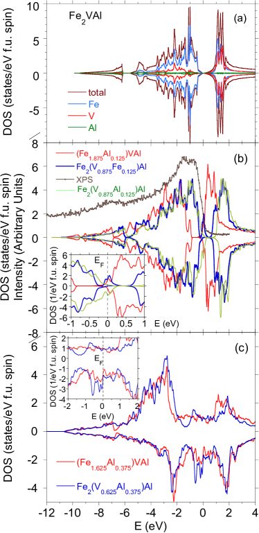
Figure 18: (a) Calculated total and spin-resolved density of states (TDOS) within the LSDA$+U+$SO ($U=3$ eV) approximation for Fe₂VAl. Also are shown the partial TDOS calculated for Fe, V, and Al. (b) Valence band (VB) XPS spectrum for Fe₂VAl_1.35 (gray points) compared to the calculated TDOS (LSDA$+U+$SO, $U=3$ eV) for the supercell of various off-stoichiometry variants of Fe₂VAl. (c) The spin resolved TDOS within the LSDA$+U+$SO, $U=3$ eV, for (Fe₁₃Al₃)V₈Al₈ (red) and Fe₁₆(V₅Al₃)Al₈ (blue) supercells. The insets exhibit details near the Fermi level in an extended energy scale.

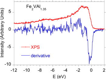
Figure 19: Valence band XPS spectrum for Fe₂VAl_1.35 (red points) and its derivative $dI/dE$ (blue line). The extreme in $dI/dE$ for $E\approx 0.2$ eV is related to Fe_AS $d$-electron states located in the electronic bands near the Fermi level.

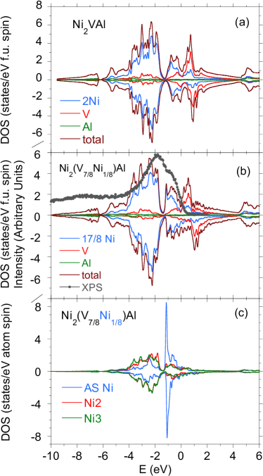
Figure 20: (a) Calculated total and spin resolved DOS within the LSDA$+U+$SO ($U=3$ eV) for Ni₂VAl. Also are shown the partial TDOS calculated for Ni, V, and Al. (b) VB XPS spectrum for Ni₂VAl_1.08 (gray points) compared to the calculated TDOS (LSDA$+U+$SO, $U=3$ eV) for Ni₁₆(V₇Ni₁)Al₈ supercell. (c) Total DOS per one atom for Ni at various sites. The blue line represents the TDOS of AS Ni defects at V sites.

Appearance of this strongly correlated $d$-like band was also reported for similar Fe₂TiSn compound due to an excess of Fe_AS atoms at Ti antisite positions [17]. The DOS of this narrow peak in the gap of the Fe₂TiSn bands is composed mainly of the $d-e_{g}$ states of Fe_AS that hybridize with the $d$ states of the eight nearest Fe atoms in octahedral coordination; moreover, the calculated magnetic structure of [Fe₁₅Ti_AS][Ti₇Fe_AS]Sn₈ is of a cluster character (more details in Ref. [57]).

The narrow $d$-band of Fe_AS is a reason of several anomalous thermodynamic properties attributed to many-body effects. For example, the mechanism of electrical transport in Fe₂TiSn with AS Fe defects has been explained as a result of interband transitions between this narrow $d$ band and other conduction states through a small gap at $\epsilon_{F}$ [57]. Here, we calculated the bands for Fe₂VAl and Ni₂VAl in various variants of their stoichiometry and in the presence of the AS structural disorder. One notes, Fe₂VAl_1.35 exhibits analogous $\rho(T)$ behavior to that of Fe₂TiSn, which suggests similar in nature electronic band properties of both the compounds.

The calculations were performed with the use of the FP-LAPW method complemented with local orbitals. The spin-orbit (SO) interaction for valence and local orbital states was taken into account, and the effective Hubbard parameter $U_{\rm eff}$ for the $d$-states of Fe, Ni, and V was assumed to be 3 eV. The super-cell methodology of alloy modeling was used to simulate the disorder. Figure 18 compares the atomic DOSs per atom for Fe₂VAl (a) with similar DOSs calculated for supercell of the off-stoichiometric Fe₂VAl analogues containing an excess of one Al atom located at Fe sites, (Fe₁₅Al₁)V₈Al₈, excess of one Fe at V sites, Fe₁₆(V₇Fe₁)Al₈, and excess of Al at V sites, Fe₁₆(V₇Al₁)Al₈, respectively (b), and off-stoichiometric analogues shown in panel (c) where three Al atoms are at Fe sites, (Fe₁₃Al₃)V₈Al₈, and three Al atoms occupy V sites, Fe₁₆(V₅Al₃)Al₈. The first variant of disorder with one atom at the AS position predicts the gap located in the electronic bands of the assumed compounds; however, its location with respect to $\epsilon_{F}$ is different depending on the atom at the AS site. Namely, when an Al atom occupies the Fe sites, the gap is located at energies $E<\epsilon_{F}$, for one Fe at V sites the gap is symmetrically located around $\epsilon_{F}$, while for scenario with one Al at V sites the gap is located just above $\epsilon_{F}$. All scenarios give narrow band states at $\epsilon_{F}$, and are possible in the off-stoichiometry sample. However, note that only the AS Fe defects at V positions lead to the appearance of a narrow $3d\uparrow$ band at $\epsilon_{F}$, which seems to be the most reasonable explanation for the experimental data shown in Fig. 14. Within this scenario, the VRH hopping throw the pseudogap $k_{B}T_{0}$ of $\sim 20$ meV, which is calculated two orders in magnitude lower than the gap of Fe₂VAl, can be possible (cf. Fig. 18(b)). It is reasonable to assume that all three DOSs shown in panel (b) contribute to the total DOS of the disordered sample with appropriate weighting factors, with the result giving an agreement of calculations with the valence XPS spectra. The DOSs calculated for the more disordered system, with the exchange of three Al atoms with Fe or V assumed, respectively, do not give a good comparison with the experiment, as shown in panel (c). The details of the DFT calculations are summarized in Table 3.

Table 3: Fe₂VAl (F$m\bar{3}m$) and the off-stoichiometric analogues; FP-LAPW results for supercell of (Fe₁₅Al₁)V₈Al₈, Fe₁₆(V₇Fe₁)Al₈, and Fe₁₆(V₇Al₁)Al₈. $n_{l}$ is a number of valence electrons, $l=0$, 1, 2, and 3 ($s$, $p$, $d$, and $f$ electron states, respectively). $m$ is total magnetic moment of each atom in the supercell.

supercell	formula unit	mtotal	DOS($\epsilon_{F}$)	$\gamma_{0}^{calc}$
		($\mu_{B}$/f.u.)	(1/eV f.u.)	(mJ/K2 mol)
	Fe2VAl	0	0	0
atom	multiplicity	$n_{s}$	$n_{p}$	$n_{d}$	$n_{f}$	mtotal/atom in $\mu_{B}$
Al	1	2.4354	6.5068	0.1094	0.0120	0.000
Fe	2	2.2332	6.1952	5.8200	0.0070	0.000
V	1	2.1458	6.0268	2.4886	0.0152	0.000
Fe15V8Al9	(Fe15/8Al1/8)VAl	0.04	1.93	4.55
atom	multiplicity	$n_{s}$	$n_{p}$	$n_{d}$	$n_{f}$	mtotal/atom in $\mu_{B}$
Fe1	1	2.24	6.20	5.83	0.01	0.155
Fe2	1	2.24	6.20	5.83	0.01	0.082
Fe3	1	2.23	6.19	5.82	0.01	-0.123
Fe4	4	2.23	6.19	5.82	0.01	-0.052
Fe5	2	2.23	6.19	5.82	0.01	-0.056
Fe6	4	2.23	6.19	5.81	0.01	0.012
Fe7	2	2.23	6.19	5.81	0.01	0.018
V1	4	2.15	6.03	2.46	0.01	0.056
V2	4	2.15	6.03	2.42	0.01	0.039
Al1	4	2.43	6.50	0.12	0.01	0.000
Al2	4	2.43	6.50	0.11	0.01	0.000
Al3	1	2.43	6.52	0.10	0.01	0.000
Fe16V7Al9	Fe2(V7/8Al1/8)Al	0.21	2.18	5.13
atom	multiplicity	$n_{s}$	$n_{p}$	$n_{d}$	$n_{f}$	mtotal/atom in $\mu_{B}$
Al1	2	2.4350	6.5119	0.1190	0.0121	-0.00574
Al2	4	2.4330	6.5040	0.1147	0.0117	-0.00542
Al3	2	2.4329	6.5037	0.1147	0.0118	-0.00509
Fe1	8	2.2284	6.1911	5.8335	0.0065	0.34381
Fe2	8	2.2332	6.1961	5.8190	0.0070	0.01825
Al4	1	2.4260	6.4748	0.1119	0.0111	-0.02047
V1	1	2.1520	6.0366	2.4217	0.0157	0.00161
V2	4	2.1508	6.0356	2.4231	0.0154	-0.16059
V3	2	2.1508	6.0357	2.4225	0.0154	-0.15168
Fe17V7Al8	Fe2(V7/8Fe1/8)Al	0.38	1.078	2.54
atom	multiplicity	$n_{s}$	$n_{p}$	$n_{d}$	$n_{f}$	mtotal/atom in $\mu_{B}$
Fe1	1	2.2377	6.1858	5.5736	0.0117	2.98449
Fe2	8	2.2261	6.1824	5.8144	0.0065	0.46897
Fe3	8	2.2292	6.1881	5.8108	0.0066	-0.41870
V1	4	2.1479	6.0294	2.4138	0.0142	-0.05980
V2	2	2.1479	6.0299	2.4149	0.0143	-0.04267
V3	1	2.1482	6.0304	2.4103	0.0145	0.29083
Al1	2	2.4315	6.4919	0.1079	0.0110	-0.00698
Al2	4	2.4317	6.4923	0.1086	0.0110	-0.00697
Al3	2	2.4300	6.4984	0.1122	0.0110	-0.00303

Table 4: Ni₂VAl (F$m\bar{3}m$) and the off-stoichiometric analogues; FP-LAPW results for supercell of Ni₁₆(V₇Ni₁)Al₈. $n_{l}$ is a number of valence electrons, $l=0$, 1, 2, and 3 ($s$, $p$, $d$, and $f$ electron states, respectively). $m$ is total magnetic moment of each atom in the supercell.

supercell	formula unit	mtotal	DOS($\epsilon_{F}$)	$\gamma_{0}^{calc}$
		($\mu_{B}$/f.u.)	(1/eV f.u.)	(mJ/K2 mol)
	Ni2VAl	0.335	3.06	7.22
atom	multiplicity	$n_{s}$	$n_{p}$	$n_{d}$	$n_{f}$	mtotal/atom in $\mu_{B}$
Ni	2	2.2946	6.2264	7.9708	0.0051	0.00649
V	1	2.1273	6.0018	2.4359	0.0103	0.29991
Al	1	2.4171	6.4704	0.0835	0.0084	-0.00541
Ni17V7Al8	Ni2(V7/8Ni1/8)Al	0.38	2.361	5.57
atom	multiplicity	$n_{s}$	$n_{p}$	$n_{d}$	$n_{f}$	mtotal/atom in $\mu_{B}$
Ni1	1	2.2244	6.1632	7.9765	0.0060	-0.01783
Ni2	8	2.2887	6.2181	7.9810	0.0055	-0.06997
Ni3	8	2.2896	6.2269	7.9605	0.0054	0.14194
V1	4	2.1293	6.0035	2.4393	0.0109	0.57564
V2	2	2.1293	6.0035	2.4417	0.0108	0.61413
V3	1	2.1294	5.9973	2.4440	0.0108	0.87389
Al1	2	2.4157	6.4562	0.0813	0.0083	-0.00698
Al2	4	2.4157	6.4564	0.0811	0.0083	-0.00753
Al3	2	2.4180	6.4798	0.0921	0.0093	-0.00782

Fig. 20 shows the valence band XPS spectra in comparison to the calculated total DOSs per formula for Ni₂VAl (a) and Ni₁₇V₇Al₈ supercell (b). This comparison clearly shows that the measured VB XPS spectra mostly reflect the $3d$ Ni and $3d$ V electronic states located between the Fermi energy and the binding energy $6$ eV. The Al $3ps$ states are located between 6 and 10 eV below $\epsilon_{F}$. One can note that the Ni AS defects do not drastically change the total DOSs of Ni₂VAl, however, they significantly contribute to the sharp $d$-electronic states at 1 eV below $\epsilon_{F}$ [in panel (c)], giving a magnetic moment of $0.14$ $\mu_{B}$ on Ni at AS positions (cf. Table 4). A localized magnetic moment calculated for AS Ni correlates well with the $\rho\sim-\ln T$ behavior, characteristic of the diluted Kondo systems (as shown in Fig. 15).

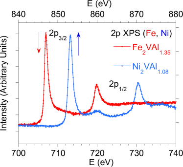
Figure 21: $2p$ XPS core level spectra for Fe in Fe₂VAl_1.35 (red) and Ni in Ni₂VAl_1.08 (blue).

Finally, we have measured the core level $2p$ XPS spectra for Fe in Fe₂VAl_1.35 and Ni in Ni₂VAl_1.08 to indirectly argument the low avarage magnetic moment of Fe and Ni in these compounds. The $2p$ XPS spectra are interpreted in reference to Refs. [73, 74], where for Mn-based Heusler alloys, it has been documented that the exchange splitting of the $2p_{3/2}$ level is directly correlated with the value of local magnetic moment at the Mn site. Specifically, the $2p_{3/2}$ splitting energy $\Delta E$ plotted as $\Delta E$ versus magnetic moment $\mu_{Mn}$ of Mn for a series of various Mn-based Heusler alloys exhibits a universal linear dependence, which gives for $\mu_{Mn}\sim 3$ $\mu_{B}$ a value of $\Delta E\sim 1$ eV. This experimental observation seems to be universal, and characteristic of other $d$-electron elements with localized magnetic moment larger than 2 $\mu_{B}$/atom (cf. Ref. [75]), simultaneously the XP spectroscopy allows one to quickly demonstrate the strength of $\mu$. The $2p_{3/2}$ lines shown in Fig. 21 do not exhibit any $\Delta E$ splitting, which suggests a nonmagnetic ground state or strongly delocalized $d$-electronic states or both, or that the magnetic moment localized on Fe and Ni, respectively, is not large enough to observe the splitting.

V Concluding remarks

Spin fluctuations in itinerant electron systems could give predominant effects on the thermodynamic properties of wealky or nearly ferromagnetic metals [42]. In consequence of the appearance of spin fluctuations, one expects an enhance of electronic specific heat, Pauli susceptibility, as well as a strong enhance of the thermopower. For many reasons, the disordered Fe₂VAl has been a candidate for good thermoelectric properties. In several previously published papers, the thermoelectric properties have been studied, either experimentally and theoretically [41, 76, 5] for pure Fe₂VAl and with dopants, however, the effect did not meet expectations. We investigated the off-stoichiometric Fe₂VAl_1.35 with excess of Al, however, the sample is not appropriate for thermoelectric applications. However, the sample is extremely interesting because of the complex magnetic properties caused by disorder. We documented the impact of AS disorder on the appearance of magnetic moment on Fe in AS positions, which in consequence leads to appearance of Griffiths phase state below $T_{G}\approx 200$ K, and singular properties in low-temperature susceptibility. In the paramagnetic regime inverse susceptibility of Fe₂VAl_1.35 obeys the Curie-Weiss law, while below a characteristic temperature $T_{G}$ $1/\chi$ displays a downward deviation from the CW law with evidently field dependent behavior, indicating the onset of short-range ferromagnetic correlation well above $T_{C}^{g}$, which is considered a hallmark of Griffiths singularity.

The DFT calculations were carried out for the disordered Fe₂VAl and its off-stoichiometric variants. The ab initio calculations predicted the Fe₂VAl compound to be nonmagnetic narrow-gap semiconductor, while for similar disordered and/or off-stoichiometric alloys Fe occupying the AS V sites is always calculated magnetic. Both band structure calculations and magnetic measurements showed at most one AS Fe defect per unit cell; therefore, the system can be treated as dilute. In result, the Griffiths phase state is possible in such a diluted system due to the finite probability of randomly large, pure, and differently diluted clusters. This result allowed us to simulate the magnetization versus temperature within the Ising model in an external magnetic field, in good agreement with the experimental data shown in Fig. 3.

The physical properties of Fe₂VAl_1.35 are analyzed with respect to paramagnetic Ni₂VAl. Up to now, this compound has not been sufficiently well investigated, more of its possible behaviors have been predicted from DFT calculations [77, 78, 79, 80]. We present comprehensive thermodynamic investigations as well as transport properties for this compound. Our DFT calculations predict magnetic moment on Ni at AS V sites, which is a reason of appearance of Kondo diluted effect in the low-temperature resistivity of Ni₂VAl, however, the superconductivity demonstrated by ab initio calculations, as was reported by Sreenivasa et al. [78], has not been confirmed experimentally for this compound.

Appendix A Numerical analysis

In Sec. III.1 we argue that the deviation from the CW law is driven by the formation of ferromagnetic clusters. As discussed in Sec. IV, ab initio calculations indicate the presence of magnetic moments on wrong-site iron atoms. The divergence of susceptibility $\chi$ (cf. Fig. 2) suggests a ferromagnetic interaction between them. However, since down to the lowest temperatures studied, the system is in the paramagnetic state, those moments are too diluted to develop a ferromagnetic state. Moreover, as can be seen in Fig. 3a), $\chi(T)$ clearly deviates from the Curie law $\chi_{C}\propto T^{-1}$, which we attribute to magnetic clusters formed in the Griffiths phase. To support this assumption, we performed Monte Carlo simulations for small magnetic clusters to determine the temperature dependence of their contribution to the bulk magnetic susceptibility. We assume that the main signal comes from the bulk of the system and fulfills the Curie law, so determine the contribution from magnetic clusters, in Fig. 22a) we present the difference between the measured susceptibility $\chi$ and $\chi_{C}$ for different values of the magnetic field.

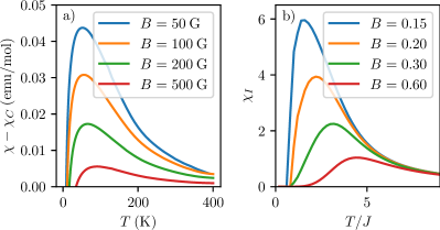
Figure 22: a) Difference between the measured susceptibility $\chi(T)$ and susceptibility given by the Curie law $\chi_{C}$. Only part for $\chi>\chi_{C}$ is shown. b) Magnetic susceptibility $\chi_{I}$ of a $2\times 2\times 2$ Ising model in external magnetic field.

In Fig. 22b), for comparison, we present a temperature dependence of the magnetic susceptibility of a very small ($2\times 2\times 2$) cluster described by the Ising model in an external magnetic field. However, there are two differences between these two results. The first is related to the behavior at low temperatures. On the one hand, the measured susceptibility $\chi$ remains finite when $T\to 0$, while $\chi_{C}$ diverges as $T^{-1}$. Therefore, $\chi-\chi_{C}$ goes to $-\infty$ when $T\to 0$ (only $\chi>\chi_{C}$ is shown in Fig. 22a). On the other hand, the susceptibility $\chi_{I}$ of the Ising model goes to zero when $T\to 0$. This discrepancy can result from approximations/limitations applied to $\chi-\chi_{C}$, e.g., instead of the Curie law, the bulk susceptibility can be described by the Curie-Weiss law with $\theta_{\rm CW}<0$ which does not have a singularity at $T=0$. The other difference between panels a) and b) of Fig. 22 can be seen at high temperature, where $\chi_{I}$ is almost temperature independent, while $\chi-\chi_{C}$ decreases with increasing temperature. This discrepancy can result from neglecting other contributions to the magnetic susceptibility, e.g., the effect of spin fluctuations. The qualitative differences between the shapes of the lines are also due to the vast simplification of considering only one size of the clusters. In the Griffiths phase we expect an ensemble of clusters of different sizes with their distribution depending on temperature. Moreover, we took into account the simplest possible kind of magnetic interactions in the cluster, i.e, the Ising model. This simplification does not allow for different magnetization orientations in different clusters, which is expected because of the complex nature of the RKKY interaction. However, the qualitative agreement of the temperature dependencies of $\chi-\chi_{C}$ and $\chi_{I}$ we observe despite the use of strong approximations applied both to $\chi-\chi_{C}$ and to the modeled $\chi_{I}$ is a strong argument for the presence of magnetic clusters in the system.

^⋆Author to whom correspondence should be addressed: andrzej.slebarski@us.edu.pl

- [1] C. Felser and A. Hirohata, Heusler Alloys: Properties, Growth, Applications (Springer International Publishing, 2016).
- [2] S. Chatterjee, S. Chatterjee, S. Giri, and S. Majumdar, J. Phys.: Condens. Matter, 34 , 013001 (2022).
- [3] T. Klimczuk, C. H. Wang, K. Gofryk, F. Ronning, J. Winterlik, G. H. Fecher, J. -C. Griveau, E. Colineau, C. Felser, J. D. Thompson, D. J. Safarik, and R. J. Cava, Phys. Rev. B 85, 174505 (2012).
- [4] Z. Lin, E3S Web of Conferences 213, 02016 (2020).
- [5] D. Bourgault, H. Hajoum, S. Pairis, O. Leynaud, R. Haettel, J. F. Motte, O. Rouleau, and E. Alleno, ACS Appl. Energy Mater. 6, 1526 (2023); and references cited therein.
- [6] K. Sato, T. Naka, M. Taguchi, T. Nakane, F. Ishikawa, Y. Yamada, Y. Takaesu, T. Nakama, A. deVisser, and A. Matsushita, Phys. Rev. B 82, 104408 (2010).
- [7] A. Ślebarski and J. Goraus, Phys. Rev. B 80, 235121 (2009).
- [8] T. Naka, K. Sato, M. Taguchi, T. Nakane, F. Ishikawa, Y. Yamada, Y. Takaesu, T. Nakama, and A. Matsushita, Phys. Rev. B 85, 085130 (2012).
- [9] T. Naka, A. M. Nikitin, Yu Pan, A. de Visser, T. Nakane, F. Ishikawa, Y. Yamada, M. Imai, and A. Matsushita, J. Phys.: Condensed Matter, 28, 285601 (2016).
- [10] R. Weht and W. E. Pickett, Phys. Rev. B 58, 6855 (1998).
- [11] D. J. Singh and I. I. Mazin, Phys. Rev. B 57, 14352 (1998).
- [12] G. Y. Guo, G. A. Botton, and Y. Nishino, J. Phys.: Condens. Matter. 10, L199 (1998).
- [13] T. Graf, C. Felser, and S. S. Parkin, Prog. Solid State Chem. 39, 1 (2011).
- [14] I. Galanakis, P. H. Dederichs, and N. Papanikolaou, Phys. Rev. B 66, 174429 (2002).
- [15] Y. Nishino, H. Kato, M. Kato, and U. Mizutani, Phys. Rev. B 63, 233303 (2001).
- [16] A. Matsushita, T. Naka, Y. Takano, T. Takeuchi, T. Shishido, and Y. Yamada, Phys. Rev. B 65, 075204 (2002).
- [17] A. Ślebarski, J. Phys. D: Appl. Phys. 39, 856 (2006).
- [18] R. B. Griffiths, Phys. Rev. Lett. 23, 17 (1969).
- [19] Griffiths observed a nonanalytic behavior of the magnetization above Curie temperature in a randomly diluted Ising ferromagnet, caused by the formation of ferromagnetic clusters above [18]. This intermediate phase between the ferromagnetic and paramagnetic phases is referred to as the Griffiths phase.
- [20] F. S. da Rocha, G. L. F. Fraga, D. E. Brandão, c. M. da Silva, and A. A. Gomes, Physica B 269, 154 (1999).
- [21] Z. Wen, Y. Zhao, H. Hou, B. Wang, and P. Han, Materials and Design 114, 398 (2017).
- [22] Y-K Wang and J-Ch Tung, Physics Open, 2, 100008 (2020).
- [23] P. V. Sreenivasa Reddy, V. Kanchana, G. Vaitheeswaran, and D. J. Singh, J. Phys.: Condens. Matter 28, 115703 (2016).
- [24] J. Rodriguez-Carvajal, Physica B 192, 55 (1993).
- [25] B. H. Toby, Powder Diffr. 21, 67 (2006).
- [26] D. J. Singh, L. Nordstrom Plane Waves, Pseudopotentials, and the LAPW Method (2nd edition), Springer Science (2006), ISBN 978-0-387-28780-5.
- [27] P. Blaha, K. Schwarz, G. K. H. Madsen, D. Kvasnicka, and J. Luitz, WIEN2k, An Augmented Plane Wave + Local Orbitals Program for Calculating Crystal Properties (Karlheinz Schwarz, Techn. Universität Wien, Austria, 2001).
- [28] J. P. Perdew, K. Burke, and M. Ernzerhof, Phys. Rev. Lett. 77, 3865 (1996).
- [29] V. I. Anisimov, J. Zaanen, and O. K. Andersen, Phys. Rev. B 44, 943 (1991).
- [30] V. I. Anisimov, I. V. Solovyev, M. A. Korotin, M. T. Czyżyk, G. A. Sawatzky, Phys. Rev. B 48, 16929 (1993).
- [31] V2FeAl is a well known Pauli paramagnet, however, its magnetic properties sensitively depend on the degree of atomic order on the different crystallographic sites. The ground state of V2FeAl, obtained experimentally and from the ab-initio calculations [32] is determined weakly magnetic for various structural models, which means that the disorder induces the short-range magnetic ordering below about 220 K.
- [32] R. Smith, Z. Gercsi, R. Zhang, K. E. Siewierska, K. Rode, and J. M. D. Coey, https://arxiv.org/pdf/2309.11480v1.pdf
- [33] S. Chatterjee1, S. Giri1, S. Majumdar, P. Dutta, P. Singha, and A. Banerjee, 34, 295803 (2022).
- [34] A. Ślebarski, J. Goraus, and M. Fijałkowski, Phys. Rev. B 84, 075154 (2011).
- [35] A. J. Bray, Phys. Rev. Lett. 59, 586 (1987).
- [36] R. Shankar and G. Murthy, Phys. Rev. B 36, 536 (1987).
- [37] M. Randeria, J. P. Sethna, and R. G. Palmer, Phys. Rev. Lett. 54, 1321 (1985).
- [38] A. H. Castro Neto, G. Castilla, and B. A. Jones, Phys. Rev. Lett. 81, 3531 (1998).
- [39] A. K. Pramanik and A. Banerjee, Phys. Rev. B 81,024431 (2010).
- [40] Y. Nishino, M. Kato, S. Asano, K. Soda, M. Hayasaki, and U. Mizutani, Phys. Rev. Lett. 79, 1909 (1997).
- [41] N. Tsujii, A. Nishide, J. Hayakawa, and T. Mori, Sci. Adv. 5, 5935 (2019).
- [42] T. Moriya, Spin Fluctuation in Itinerant Electron Magnetism (Springer-Verlag, Berlin Heilderberg, 1985).
- [43] T. Takahashi, Spin Fluctuation Theory of Itinerant Magnetism (Springer-Verlag Berlin Heidelberg, 2013).
- [44] A. J. Cox, J. G. Louderback, S. E. Apsel, and L. A. Bloomfield, Phys. Rev. B 49, 12295 (1994).
- [45] M. Castro, C. Jamorski, and D. R. Salahub, Chem. Phys. Lett. 271, 133 (1997).
- [46] Y. Jo, M. H. Jung, M. C. Kyum, K. H. Park, and Y. N. Kim, J. Magnetics, 11, 156 (2006).
- [47] J. A. Mydish, Spin Glasses: An Experimental Introduction (Taylor and Francis, London, 1993.
- [48] corresponds to Debye-type exponential relaxation, for , there is no relaxation at all.
- [49] R. S. Freitas, L. Ghivelder, F. Damay, F. Dias, and L. F. Cohen, Phys. Rev. B 64, 144404 (2001).
- [50] A. H. Castro Neto and B. A. Jones Phys. Rev. B 62, 14975 (2000).
- [51] P. Levy, F. Parisi, L. Granja, E. Indelicato, and G. Polla, Phys. Rev. Lett. 89,137001 (2002).
- [52] S. Harikrishnan, S. Rößler, C. M. N. Kumar, Y. Xiao, H. L. Bhat, U. K. Rößler, F. Steglich, S. Wirth, and S. Elizabeth, J. Phys.: Condens. Matter 22,346002 (2010).
- [53] A.Tari, The Specific Heat of Matter at Low Temperatures, Imperial College Press, London 2003.
- [54] C.S. Lue, J.H. Ross, Jr, C.F. Chang and H.D. Yang, Phys. Rev. B 60, R13941 (1999).
- [55] C.S. Lue, H.D. Yang, and Y.K. Kuo, Chinese Journal of Physics 43, 775 (2005).
- [56] K. Ikeda, S. K. Dhar, M. Yoshizawa, and K. A. Gschneidner, Jr., J. Magn. Magn. Mater. 100, 292 (1991).
- [57] A. Ślebarski, J. Deniszczyk, W. Borgieł, A. Jezierski, M. Swatek, A. Winiarska, M. B. Maple, and W. M. Yuhasz Phys. Rev. B 69, 155118 (2004).
- [58] J. Spałek, European J. Phys. 21, 511 (2000).
- [59] K. D. Schotteand U. Schotte, Phys. Lett. A 55, 38 (1975).
- [60] H. -U. Desgranges and K. D. Schotte, Phys. Lett. A 91, 240 (1982).
- [61] O. Trovarelli, J. G. Sereni, G. Schmerber, and J. P. Kappler, Phys. Rev. B 49, 15179 (1994).
- [62] F. Garmroudi, M. Parzer, A. Riss, A. V. Ruban, S. Khmelevskyi, M. Reticcioli, M. Knopf, H. Michor, A. Pustogow, T. Mori, and E. Bauer, Nature Communications 13, 3599 (2022).
- [63] T. Okabe, J. Phys.: Condens. Matter 22, 115604 (2010).
- [64] E. Gratz, A. S. Markosyan, J. Phys.: Condens. Matter 13, R385 (2001).
- [65] A. Ślebarski,, J. Goraus, J. Deniszczyk, and Ł. Skoczeń, J. Phys.: Condens. Matter 18, 10319 (2006).
- [66] A. Ślebarski, M. B. Maple, E. J. Freeman, C. Sirvent, D. Tworuszka, M. Orzechowska, A. Wrona, A. Jezierski, S. Chiuzbaian, and M. Neumann, Phys. Rev. B 62, 3296 (2000).
- [67] S. Chaudhuri, P. A. Bhobe1, A. Bhattacharya, and A. K. Nigam, J. Phys.: Condens. Matter 31, 045801 (2019).
- [68] N. F. Mott, Phil. Mag. 13, 989 (1966).
- [69] N. F. Mott, Metal-Insulator Transitions (Taylor and Francis LTD, London, 1974).
- [70] J. Delahaye, J. P. Brison, and C. Berger, Phys. Rev. Lett. 81, 4204 (1998).
- [71] P. Schlottmann, Z. Phys. B: Condens. Matter 51, 223 (1983).
- [72] J. Deniszczyk, Acta Phys. Pol. B 32, 529 (2001).
- [73] Yu. M. Yarmoshenko1, M. I. Katsnelson1, E. I. Shreder, E. Z. Kurmaev, A. Ślebarski, S. Plogmann, T. Schlathölter, J. Braun, and M. Neumann, Eur. Phys. J. B 2, 1 (1998).
- [74] S. Plogmann, T. Schlathölter, J. Braun, M. Neumann, Yu. M. Yarmoshenko, M. V. Yablonskikh, E. I. Shreder, E. Z. Kurmaev, A. Wrona, and A. Ślebarski, Phys. Rev. B 60, 6428 (1999).
- [75] A. Ślebarski, M. Neumann, and B. Schneider, J. Phys.: Condens. Matter, 13, 5515 (2001).
- [76] G. A. Naydenov, P. J. Hasnip, V. K. Lazarov, and M. J. Probert, J. Phys.: Condens Matter. 32, 125401 (2020).
- [77] F. S. da Rocha, G. L. F. Fraga, D. E. Brando, C. M. da Silva, and A. A. Gomes, Physica B 269, 154 (1999).
- [78] P. V. S. Reddy, V. Kanchana, G. Veitheeswaran, and D. J. Singh, J. Phys.: Condens Matter. 28, 115703 (2016).
- [79] Z. Wen, Y. Zhao, H. Hou, B. Wang, and P. Han, Materials and Design, 114, 398 (2017).
- [80] Y. -K. Wang and J. -Ch. Tung, Physics Open 2, 100008 (2020).