Active Inference Demonstrated with Artificial Spin Ice

Abstract

A variational Bayesian method is implemented in a numerical model of interacting nanomagnetic elements to demonstrate active inference in an Artificial Spin Ice geometry. It is shown that thermal fluctuations can drive this magnetic spin system to evolve along a trajectory of spin configuration states in response to an external environment according to a neurological free energy principle with active inference. The proposed bilayer is an extension of a two-dimensional system studied in an Artificial Spin Ice that has been extensively investigated experimentally and theoretically. The two layers function effectively as a sensory layer providing input to a hidden layer. The spin dynamics displayed by the bilayer are shown to be well described using a continuous form of the free energy principle that has been proposed as a high level description of certain biological neural processes. Numerical simulations demonstrate that this proposed bilayer geometry is able to reproduce theoretical results derived previously for examples of neurological action and perception.

I Introduction

In recent years a high level approach to the understanding of certain neuralogical functions has been proposed that is based on the concept of active inference and a free energy principle. Active inference and the free energy principle refer to a mathematical description of neural dynamics in biological systems. [1] The approach appears able to provide a biologically plausible mechanism that can describe many aspects of motor control in biological systems. [1, 2, 3, 4, 5] A fundamental hypothesis is that many brain functions can be understood as Bayesian inference and discrete and continuous formulations of the mathematical formalism have been developed. [6, 7, 8]

There is a long history of using binary spins in models for neural operations [9] and theories for their operation in neural networks (for example as discussed in [10] and references therein). In the present paper, an Ising spin model is proposed that behaves as predicted by active inference theory according to the continuous formulation of the neurological free energy principle. The spins in the present model are nanomagnets arranged in geometries related to those first explored for Artificial Spin Ice.

Artificial Spin Ice has proven useful for investigations of complex frustrated systems from theoretical and experimental perspectives. [11, 12] One of the benefits has been to provide experimental models that can be probed with unprecedented detail on time and length scales that are not otherwise ammenable to study. [13] Some of the most recent developments include neuromorphic applications for machine learning [14, 15, 16] and fabrication of non-trivial three dimensional structures in complex geometries [17, 18] .

The structure assumed throughout this paper is a three dimensional bilayer array of nanomagnets and is a modification of a geometry suggested in [19]. The geometry studied here uses nanomagnets in one layer as super-paramagnetic sensory receptors that are able to communicate information from the environment to the remaining set of strongly interacting nanomagnets that are otherwise mostly hidden from the environment. The configurations of this hidden set of spins evolve thermally and their average magnetization provides a signal which is fed back to the environment in order to control future input to the sensory spins. Viewed on the time scale of the environment, the average magnetization produced by the hidden layer follows a trajectory that can converge to the neighbourhood of a predetermined desired value.

The purpose of this paper is to propose this system as an example of a class of three dimensional thermally active nanomagnet arrays that can serve as plattforms for experimental study of active inference. It is shown that the behaviour displayed by this system is accurately described by the free energy principle formulation for continuous dynamics and that the formalism provides a useful means of describing complex out-of-equilibrium non-linear dynamics which evolves on internal timescales that can differ from the timescale in which the environment evolves.

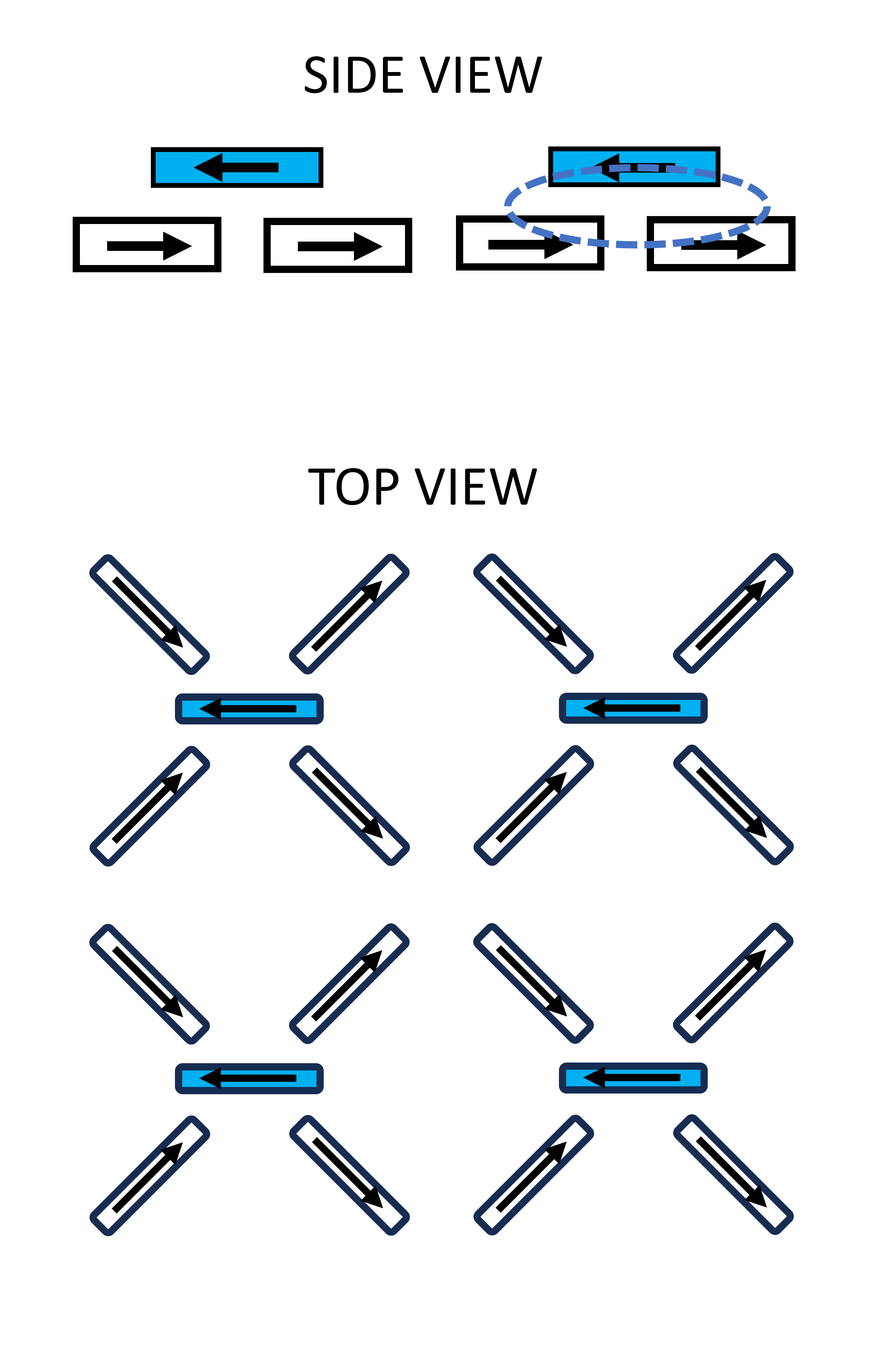
Figure 1: Geometry of a bilayer Artificial Spin Ice for use in active inference composed of small magnetic elements. The top layer of spins (shaded blue in the figure) are placed above the vertices of the so-called ’square’ Artificial Spin Ice geometry (unshaded). The top layer elements are assumed to interact with the bottom layer through stray magnetic fields but are assumed sufficiently distant from one another not interact strongly between themselves. The top layer spins are aligned by a magnetic field applied locally to only the top layer by the external environment and referred to as ’sensory spins’. The bottom layer of spins interact strongly with one another but are assumed to not experience the field applied to the sensory spins. These are called ’hidden spins’.

II Nanomagnet Model

The nanomagnet array proposed in this paper is sketched in  1. The magnetic properties of the nanomagnets are assumed to be ferromagnetic below a critical temperature $T_{c}$ and align spontaneously along the long axis of the particle. The particles are assumed to be sufficiently small that the magnetisation approximates an Ising spin with thermally driven reversals of direction at temperatures well below $T_{c}$. Furthermore, the spacing between elements in the arrays are sufficiently small that magnetic stray fields produced by the nanomagnets are can affect the probability of reversal for neighbouring nanomagnets. Such systems have been produced experimentally and reversal processes studied experimentally. Theoretical models using Ising spins to represent the nanomagnets are able to describe most features qualitatively well but neglect effects that result from micromagnetic deviations from Ising-like behavour.

There are two different arrays of spins shown in the structure of Fig.  1. The larger array of $16$ spins is called a ’square ice’ geometry and is known to have a two-fold degenerate ground state that in which the average direction spins cancel for a net zero magnetization of the array. The ground states can be characterized by the so-called ’ice rule’ which requires two spins at each vertex to point inwards towards the vertex centre with the remaining two spins pointing out from the vertex. The stability of vertex spin configurations depends on temperature as thermal fluctuations have a finite probabilty to reverse spins randomly.

A main purpose of this paper is to examine how local fields induced in the Artificial Spin Ice can be used to manipulate its relaxation dynamics. In real systems this may achieved in a number of ways that are in principle similar to writing and erasing data in magnetic media. Here a scheme is proposed that would make use of additional magnetic elements positioned in a layer separate from the Aritifical Spin Ice. The requirements for spins in this layer are that they do not reverse as easily as the spins in the other layer and are assumed to align independently of both the larger array and also independently of one another. Their alignment is assumed to be subject to some externally applied local magnetic field and in this way they act as sensors of this external field. Their alignment with the external field is stochastic in that each spin has only a finite probability of aligning with the external field. In this regards, the sensory and hidden layer spins experience different effective temperatures.

The dipolar interactions between spins in the bilayer are calculated using a dumbbell model which takes into account the length of the nanomagnet elements. [20] The geometry used for the hidden spins is defined by a square lattice of lattice constant $a$ with elements of length $\ell=a/2$ aligned diagonally within each unit cell. The fields produced by the sensory spins have strength at the hidden spin layer that depends on the separation between the two layers. The separation assumed throughout this paper is $a/10$. Each element has a magnetic moment $m_{\alpha}=\mu_{0}V_{\alpha}\rho_{\alpha}$ where $\alpha$ is either $s$ or $h$ depending on the layer, $V_{\alpha}$ is the element volume and $\rho_{\alpha}$ is the element moment density.

The probability of a spin reversal in a nanomagnet at a given temperature and local field depends on several geometrical and material factors. These effects can be captured by defining effective temperatures for each of the two layers that include the magnetic moment of the magnetic elements. The spins in the sensory layer are simulated at an effective temperature ${\beta_{s}}^{-1}=k_{B}T_{s}/m_{s}$ and the effective temperature of the hidden spins is ${\beta_{h}}^{-1}=k_{B}T_{h}/m_{h}$ where $k_{B}$ is the Boltzmann constant.

The energy used for Monte Carlo simulations includes field and dipole interaction terms acting at each spin and is used to determine the energy change $\Delta E$ for a possible spin reversal at each site. Using notation $\beta_{s}$ and $\beta_{h}$ for the inverse temperatures of the sensory and hidden layers respectively, and also locations ${r}_{s}$ for a site in the sensory layer and ${r}_{h}$ in the hidden layer, the approximate energy change for a sensory spin $\omega_{s}(r_{s})$ is:

$$\begin{split}\Delta E(r_{s})=&2\beta_{s}\Bigg{\{}\Bigg{.}-h_{e}\sigma_{s}(r_{s})+\sigma_{s}(r_{s})\sum_{{r^{{}^{\prime}}}_{s}}D(r_{s}-{r^{{}^{\prime}}}_{s})m_{s}\sigma_{s}({r^{{}^{\prime}}}_{s})+\sigma_{s}(r_{s})\sum_{{r^{{}^{\prime}}}_{h}}D(r_{s}-{r^{{}^{\prime}}}_{h})m_{h}\sigma_{h}({r^{{}^{\prime}}}_{h})\Bigg{.}\Bigg{\}}\\ \approx&2\beta_{s}\Bigg{\{}\Bigg{.}-h_{e}\sigma_{s}(r_{s})+\sigma_{s}(r_{s})\sum_{{r^{{}^{\prime}}}_{h}}D(r_{s}-{r^{{}^{\prime}}}_{h})m_{h}\sigma_{h}({r^{{}^{\prime}}}_{h})\Bigg{.}\Bigg{\}}\end{split}$$ (1)

The first term in Eq. 1 is the interaction energy of the sensory spins with the environment field and is proportional to the magnetic moment $m_{s}$ of a sensory element. The second term represents the dipole field interactions between the sensory spins. In this expression the dipolar term is a sum over the spins separated by distances $r_{ij}$ with directions specified by unit vectors for each spin $\hat{\epsilon}_{i},\hat{\epsilon}_{j}$. The dipolar interaction energy is given by $D=\mathcal{D}\sum_{i,j}[\hat{\epsilon}_{i}\cdot\hat{\epsilon_{j}}/|r_{ij}|^{3}-3(\hat{\epsilon}_{i}\cdot\vec{r}_{ij}))(\hat{\epsilon}_{j}\cdot\vec{r}_{ij}))/|r_{ij}|^{5}]$. The prefactor contains the strength of the magnetic moment and volume factors as $\mathcal{D}=\mu_{0}/4\pi a^{3}$ . All dipole sums are approximated by dumbbell charges as outlined in  [20].

The dipole term in Eq. 1 is neglected under the assumption that the environment field energy is much larger than the dipole interaction between sensory spins. An additional assumption is that the sensory magnetic moments $\sigma_{s}$ are much larger than the hidden spin magnetic moments $\sigma_{h}$. This means the $h_{e}$ term dominates except for very small $h_{e}$ and the $D$ energy contributes effectively as a small noise term. It is neglected in the numerical calculations.

The approximate energy change for a spin in the hidden layer is

$$\begin{split}\Delta E(r_{h})=&2\beta_{h}\Bigg{\{}\Bigg{.}-h_{e}\sigma_{h}(r_{h})+\sigma_{h}(r_{h})\sum_{{r^{{}^{\prime}}}_{h}}D_{\beta_{h}}(r_{h}-{r^{{}^{\prime}}}_{h})m_{h}\sigma_{h}({r^{{}^{\prime}}}_{h})+\sigma_{h}(r_{h})\sum_{{r^{`}}_{s}}D(r_{h}-{r^{{}^{\prime}}}_{s})m_{s}\sigma_{s}({r^{{}^{\prime}}}_{s})\Bigg{.}\Bigg{\}}\\ \approx&2\beta_{h}\Bigg{\{}\Bigg{.}\sigma_{h}(r_{h})\sum_{{r^{{}^{\prime}}}_{h}}D(r_{h}-{r^{{}^{\prime}}}_{h})m_{h}\sigma_{h}({r^{{}^{\prime}}}_{h})+\sigma_{h}(r_{h})\sum_{r_{s}}D(r_{s}-{r^{{}^{\prime}}}_{h})m_{s}\sigma_{s}({r^{{}^{\prime}}}_{s})\Bigg{.}\Bigg{\}}\end{split}$$ (2)

The first term in Eq. 2 is the effect of the external environment field on the hidden spins. This external field is assumed to be locally applied to the sensor spins and much smaller for the hidden spins ( smaller than the spin interaction terms) and neglected. The second term represents interactions between all spins in the hidden layer. The third term represents the fields generated by sensory spins acting on the hidden layer spins.

An important aspect of this model is that because the effective temperatures for the sensory and hidden layer spins are different, timescales for reversal dynamics are also different. These are modelled such that the sensory spins relax with respect to the instantaneous value of the external field, while the hidden spins relax in accord to the state of the sensory spins. The condition $T_{s}>T_{h}$ describes sensory spins that sample the local input field more frequently than the hidden spins sample the sensory spin configuration. In the results for the active inference experiments which follow later, a competition appears between the ability to sample configuration states and the advantages of limiting exploration of states that is dependent upon temperature.

III Properties of the Sensory Spin Layer

To understand this competition, it is helpful to first examine numerically how the bilayer structure explores configuration states of the hidden layer. For the numerical simulations reported in this paper, a $36$ element square ice is used with nine sensory control elements placed above the vertices internal to the lattice in the manner depicted in Fig. 1. The magnitude of the magnetic charge on each hidden element is set to unity and the magnitude of the magnetic charge on each element is a parameter adjusted through choice of $\beta_{s}$ and $\beta_{h}$ as discussed above. Monte Carlo sampling is made for an ensemble of $100$ identical bilayer array replicas sampled independently. The number of Monte Carlo Steps (MCS) performed during each time interval are specified separately for the sensory and hidden spins with the numbers $N_{s}$ and $N_{h}$ respectively. The algorithm used for sampling is Glauber dynamics.

The sensory spins are positioned above the vertices of the hidden spin array. This means that the stray magnetic fields produced by individual sensory spins affect most strongly the four spins that comprise the vertex below. This additional field affects the stability of the hidden four-spin vertex and will bias the probability of spin reversals for each vertex spin. In this way the sensory layer embodies some aspects of a Markov Blanket in that it mediates information that the hidden array can receive. [21, 22, 7] Information flow between the sensory and hidden spin arrays is directed in that the sensory array is designed to respond to a single external field whereas the hidden spins respond only to the individual sensory spin fields.

The importance of this sensory ’blanket’ design can be appreciated from two aspects of how states in the hidden layer are accessed by the external field. To illustrate, in Figs.  2 and  3 a comparison between the case of an external environment field applied directly to the hidden spins without sensory spin fields, and the case of only sensory spin fields acting on the hidden spins.

The response of the hidden spin array to a magnetic field applied directly to the hidden layer spins without mediation by sensory spins is shown in Fig. 2(a) and (b). The field is applied uniformly across the hidden layer. The simulation is run for $N_{h}=100$ MCS which is long enough to allow the hidden spin system to relax towards long lived meta-stable states at each applied field. In this way the simulation mimics what would be observed in an actual hysteresis experiment where the average magnetization of a material is measured for a cycled applied field in order to identify and characterize long lived metastable magnetic states.

The magnitude of the average magnetization $M$ induced at each applied field value depends on temperature. In (a) a value $T_{h}=0.4$ (in units of dumbbell interaction strength) is used which is well below the temperature at which nanomagnet correlation lengths become negligible. In (b), a temperature of $T_{h}=1.0$ is used which is still low enough to allow an average spontaneous long range order to appear in zero field and no hysteresis is visible. The dark solid lines are the $M$ averaged over all replicas. The shaded lines are the $M$ from each replica and indicate the extent over which $M$ fluctuates at this temperature. These fluctuations are most pronounced at the smallest fields as would be expected for small temperatures. Because of this, the spin configurations accessed under the directly applied field are limited and is the reason why the replica $M$’s are clustered near the replica average $M$. Fluctuations of $M$ increase with temperature as can be seen by comparing (a) to (b).

The distribution of hidden layer states at three different, but neighbouring, fields near zero field are shown in Fig. 2(c) for the case in (a), and Fig. 2(d) for the case in (b). The distribution is discrete due to the Artificial Spin Ice geometry which constrains possible configurational states. Only two of the possible states are signficantly occupied. Evidence for restricted access to possible states is evidenced by the similarity between occupied states sampled as the field changes magnitude slightly. The overall spread in states is limited in both examples and largest for the high temperature case (b). The correlation of $M$ between successive times is also less pronounced in Fig. 2(d) as compared to (c), as would be expected for wider exploration of state space at higher temperatures.

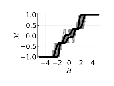
(a)

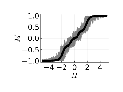
(b)

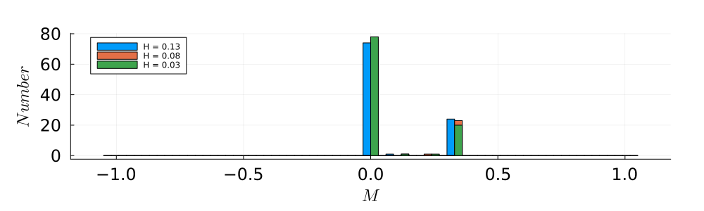
(c)

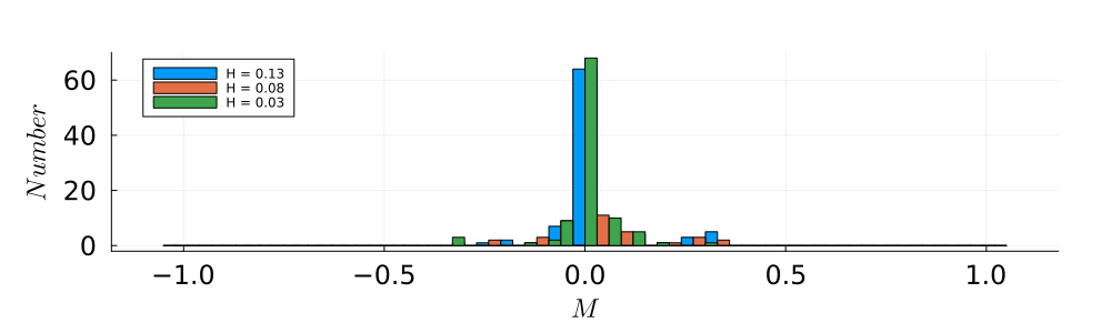
(d)

Figure 2: An external field is applied directly to the hidden spin square ice layer for numerical simulation of magnetic hysteresis. The field is applied uniformly to all of the hidden spins and response is simulated with Monte Carlo using $N_{h}=100$ and $T_{h}=0.4$ in (a) and $T_{h}=1.0$ in (b) for $700$ field steps. $N_{h}=100$ in both cases which for low temperatures is sufficient to allow the state to relax into long lived metastable states as seen by the hysteresis in $M(H)$. The states of the hidden spins are distributed as shown at small fields for three neighbouring field steps in (c), which corresponds to the low temperature case in (a). Only two significant peaks appear, one at $M=0$ and the other at $M=0.4$.

Results of using sensory spins to activate changes in the hidden spin $M$ are shown in Fig. 3. Here $N_{s}=1$ and $T_{s}=1.0$ are used. The sensory spins respond to the external applied field, but the hidden spins experience only the local fields produced by the sensory layer. In (a), $T_{h}=0.4$ and in (b) $T_{h}=1.0$ with $N_{h}$ as in Fig. 2.

The hysteresis curves shown in Fig. 3(a) and (b) are very different from the directly applied external field example. Hysteresis is visible at both temperatures and appears largest at the higher temperature. The distribution of hidden spin states for small external field values are wide. The low temperature distribution corresponding to (a) is shown in (c), and the high temperature distribution corresponding to (b) is shown in (d). In both cases the span of states goes between the maximum possible ($\pm 1$), and the higher temperature distribution occupies a greater variety states than does the distribution for lower temperature.

The differences between Figs. 2 and  3 can be understood in terms the magnetization processes responsible for changing $M$ values. The magnetic elements in the hidden layer interact strongly and alignment of magnetic element magnetization generally occurs in square ice via a type of avalanche process. When the external field is applied directly to all the square ice elements, excitation of these processes will be more likely to begin at array edges where local interations are weakest. Local fields, on the other hand, can destabilize orientations in elements away from the array edges thereby nucleating avalanche reversals within the array with greater probability.

From these examples, one can see that the sense layer provides local fields that work against the formation of meta-stable configurations but nevertheless sample states that are influenced by the existence of long lived meta-stable states. The local fields fluctuate locally at each sensory spin, but the average is consistent with the external field value. The ability to leverage multiple states through defects or direct control of artificial spin ice states was noted several years ago by Budrikis using graph theoretical methods [23, 24]. The behaviour observed in the present paper can be understood similarly in that local fields acting on a subset of spins can open pathways for avalanche processes that would otherwise have low probability of occurring. This gives access of the system to a larger portion of configurational phase space than is possible with a directly applied uniform field.

Another way of thinking of this is to consider that the spread of states sampled through the ensemble of hidden spins is wide because there exist a multitude of possible trajectories available to the correlated hidden spins as they evolve towards a lower energy configuration. This distinguishes the hidden spin system from a purely random sampling of states. A breadth of possible trajectories towards some minimal energy is fundamental to the operation of the system in the active inference applications that will be discussed later. It appears to be analagous to the requirement of sufficient memory and compute capacity required of a system suitable for reservoir computing [15].

The temporal duration of a signal is also significant and facilitated by the sensory layer. The results for an external field applied uniformly without sensory spin mediation is illustrated in Fig.  4(a). The panel on the left shows a $20$ time-step wide pulse profile as a dark black line and the magnetization $M$ averaged over all replicas of the system is shown in blue. The temperature for the square array is chosen as $T_{h}=1.0$.

The middle panel shows the cross correlation response between the pulse and the $M$ response for delay times ranging up to $15$ time steps. The correlation is normalized and calculated as described in  [15] using the definition

$$R^{2}(d)=\left[\sum_{t}\frac{(M_{t}-\langle M_{t}\rangle_{t})(p_{t}(d)-\langle p_{t-d}\rangle_{t}))}{(N-1)\sigma_{M}\sigma_{p}}\right]^{2}.$$ (3)

The averages at each time step are over the replica averaged hidden layer magnetization reponse $M_{t}$ calculated at each time step $t$ and the pulse input to the sensory spins $p_{t}$. The averages are over the time interval sampled and $\omega_{M}$ and $\omega_{p}$ are the corresponding standard deviations. The delay between $M_{t}$ and $p_{t}$ is $d$.

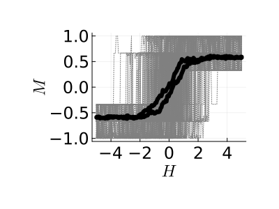
(a)

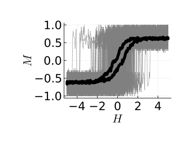
(b)

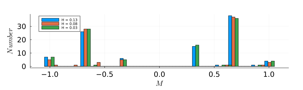
(c)

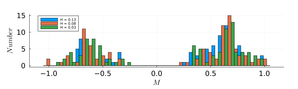
(d)

Figure 3: Hidden state response to sensory spins driven by an external field are shown in (a) for $T_{h}=0.4$ and in (b) for $T_{h}=1.0$. A value of $N_{s}=1$ is used in both cases. Hysteresis appears for each temperature and even widens at the higher temperature. The hidden spin states occupied at small external fields are shown in (c) for the low temperature case (a), and in (d) for the higher temperature case of (b). The wide distributions are because sensory spin response to the external field creates local fields in the hidden spin array that access configuration states which are not possible if the external field is applied directly and uniformly to the entire hidden spin lattice.

The cross correlation in Fig. 4(a) reaches a maximum at around six time steps into the pulse and decays rapidly after. The states accessed throughout all times are shown in the right panel and are tightly grouped around $M=0$.

The effects of sensory layer mediation are shown in Fig. 4(b) with $T_{s}=0.1$ and $N_{s}=1$. The sensory layer mediated input to the hidden spins dramatically increases sensitivity to the pulse. The correlation $R^{2}$ (middle panel) and distribution of states (right panel) show a delayed but significant response to the onset of the pulse with a clear asymmetry for $M=-1$ which corresponds to the pulse.

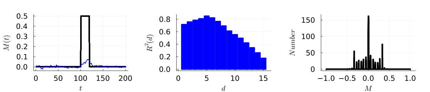
(a)

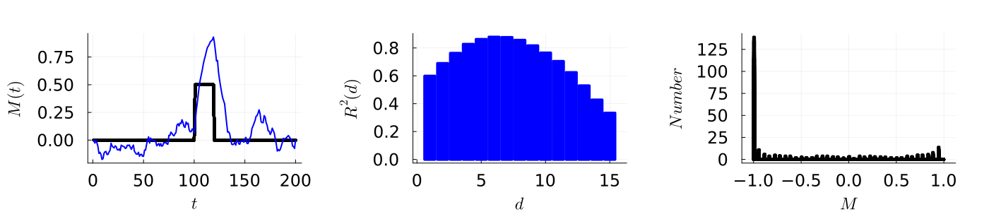
(b)

Figure 4: Pulse field profile and averaged $M$ response are shown in the left panels. Cross-correlation is shown in the middle panels, and the distribution of hidden spin states is shown in the rightmost panels. In (a) a $20$ time step wide pulse is applied as directly without sensory spin mediation. In (b) the pulse is delivered to the hidden spin layer via the sensory spin layer. The sensory spin $N_{s}=1$.

Results of longer integration time of $N_{s}=10$ is shown in Fig.  5(a). The response is now better synchronized with the pulse as can be seen from the response profile and the $R^{2}$ correlation. The distribution of states has spread states away from the $M=-1$ value compared to the $N_{s}=1$ case.

Lastly, in Fig. 5(b) sensitivity by sensory layer mediation is illustrated. In this figure the response function width is reduced from $20$ to $4$ time steps. The response to a directly applied external field (not shown) is very weak, but response is substantial when done through the sensory local field (with $N_{s}=10$) as seen in the left panel profiles. Strong correlation with the pulse remains and the distribution of states is similar to that in (a).

This sensitivity to changes in external field and the ability to activate a breadth of states is perhaps central to the operation of the system for active inference. As discussed earlier, the sensory layer creates local fields that, through avalanche dynamics, instigate configurational changes that drive the system through hidden spin state phase space. In what follows, it will be seen that this sensitivity enables the system to search widely for configurations that, when active inference is enabled, direct the hidden spin evolution trajectory towards target goals.

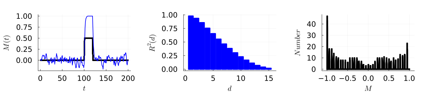
(a)

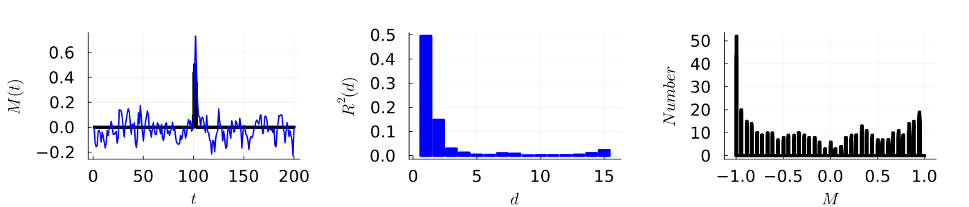
(b)

Figure 5: As in Fig. 4, the pulse field profile and averaged $M$ response are shown in the left panels. Cross-correlation is shown in the middle panels, and the distribution of hidden spin states is shown in the rightmost panels. In (a) the pulse is delivered to the hidden spin layer through the sensory spin layer. In (b) $N_{s}=10$ and the pulse width is $4$.

IV Sampling the Variational Free Energy and Implementation of Active Inference

Some definitions are required to describe how the bilayer system can perform active inference. The continuous approach formulated in terms of stochastic differential equations and used here was proposed by Friston [25]. Only a summary of essential points is presented in the present paper as the complete theory for this is well described elsewhere. The formulation and examples presented below primarily follow the description presented in [26].

Variables are defined in terms of generalized coordinates which facilitate the multiple timescale feature highlighted earlier. The external environment defines a time sequence which is regularly sampled by the sensory spins. The sampled environment consists of data that specifies a trajectory and includes the position $x(t)$ and any number of higher order derivatives $d^{n}x(t)/dt^{n}$ of $x(t)$. These can be thought of as a vector $\tilde{x}$ of data values where each component is a derivative with respect to $t$. To simplify the notation, a component of $\tilde{x}$ is denoted by $x_{\alpha}=d^{\alpha}x/dt^{\alpha}$. There is a notable feature of this representation in that the action of a derivative on $\tilde{x}$ is defined as the promotion of a component to its next higher order derivative component. This operation is denoted by the operator $D$ where $Dx_{\alpha}\rightarrow x_{\alpha+1}$ within the same vector component set $\tilde{x}$.

The configurational states of the sensory spins create a mapping to the sample environment with a component of $\tilde{\phi}$ corresponding to a component of $\tilde{x}$ at time $t$. A sensory state $\phi_{\alpha}$ is sampled during a MCS of the sensory spins in the presence of the external environment magnetic field representing a component of $\tilde{x}$. The value assigned to $\phi$ is an average over $N_{s}$ MCS for the ensemble of system replicas. An average so generated is made for each member of $\tilde{x}$ are thereby mapped to the corresponding values of $\tilde{\phi}$.

In a like manner, state averages $\tilde{\mu}$ are defined for the hidden spins where an average of an ensemble of hidden spin states is mapped to the $x(t)$ data transmitted through the sensory spins consistent via $\phi$. Note that the timescale for this mapping is not specified by a particular $t$, but depends on the number of MCS taken during a particular $t$. This provides an interesting separation of time scales between the changing values of the $\tilde{x}$ that occur on environment time, and the response of the bilayer components which is happening during stochastic thermal relaxation processes.

It is useful to note that the probability for a thermal reversal in a time interval $\Delta t$ depends not only on the energy difference between an initial and possible final state, but also on the frequency of attempt in reaching the final state. This can be described by the Arhenius equation, $\frac{1}{\tau}exp(-\beta\epsilon)$ where $\beta$ is an inverse temperature and $\epsilon$ is the energy difference between states and $1/\tau$ is an attempt frequency which measures the number of pathways to an energy barrier relative to the number of pathways across the barrier. The Monte Carlo algorithm used here does not take $\tau$ into account directly. However the number of MCS determine to what degree configurations sampled during one $\Delta t$ time step are correlated with those of the previous time step. This is a very rough analogy to the prefactor $1/\tau$ but at least captures some sense of different timescales for relaxation that two spin layers follow. Larger MCS numbers correspond to less memory from one time step (determined by the external environment field) to the next. These parameters thereby determine the rates at which the spin system layers remain coherent over time with respect to the environment clock determined by $\Delta t$. As will be seen later, $N_{s}$ and $N_{h}$ are important for optimizing performance of the bilayer system for active inference.

During thermal relaxation, the $\tilde{\mu}$ change by state transitions to new average energies. A variational Bayes relaxation is used to infer the best estimate of the distribution describing the joint probability $P(\mu,\phi)$ of having a state $\mu$ when the sensory spins are in a state $\phi$. The algorithm for this describes evolution of a trajectory for each component of $\tilde{\mu}$ defined by

$$\frac{d\mu_{\alpha}}{dt}-D\mu_{\alpha}=-\kappa\frac{\partial}{\partial\mu_{\alpha}}E(\tilde{\mu},\tilde{\phi})$$ (4)

The quantity $E(\tilde{\mu},\tilde{\phi})$ plays the role of a negative entropy defined in ensemble learning [26]. In this approach, a distribution $P(\mu,\phi)\sim\exp(-\beta E(\tilde{\mu},\tilde{\phi}))$ is used in an estimate for the unknown joint probability relating hidden to sensory states.

In the context of the spin bilayer, this corresponds to the condition where thermally driven dynamics of an average magnetization of the hidden spins responds to the fields produced by the sensory spins. Viewing $E(\tilde{\mu},\tilde{\phi})$ as an energy associated with the bilayer system, the gradient suggests an interpretation of the right hand side as a conjugate field to $\mu_{\alpha}$ driving the states of the hidden spins along a trajectory that leads to the condition $\frac{d\mu_{\alpha}}{dt}-D\mu_{\alpha}=0$. This condition describes a trajectory through state phase space where the time evolution of the average $\tilde{\mu}$ is directed towards the peak of the distribution being inferred.[27]

These ideas are illustrated through results presented below. The first example is for tracking of the magnetization to a target parameter value subject to unknown (to the bilayer spins) external constraints imposed by the environment.

The first example is set up in the following manner. The model is adapted from one given by Baltieri  [28]. The environment is defined by a one dimensional equation of motion specified as

$$\frac{dx(t)}{dt}=-\gamma x(t)+a(t).$$ (5)

This equation describes dissipative motion along $x$ that would decay to zero via a friction $\gamma$ unless offset by a term $a(t)$. The target specifies a fixed velocity $dx/dt=v_{d}$ the system should arrive to as it relaxes to the condition $\frac{d\mu_{\alpha}}{dt}-D\mu_{\alpha}=0$.

The bilayer sensory spins receive information about position and velocity through generalized coordinate vectors $\tilde{x}={x(t),dx(t)/dt}$ at regular time steps [27, 29]. A separate spin bilayer will be employed for each component of $\tilde{x}$. In each bilayer, the hidden spins will respond with a magnetization field $M_{\alpha}$ that is defined by an ensemble average over a quantity $\chi(B_{\alpha})$

$$M_{\alpha}=\langle\chi(B_{\alpha})\rangle_{T},$$ (6)

where the function $\chi$ is the magnetization measured along one direction of the spin lattice array subject to a field $B_{\alpha}$. The average $M_{\alpha}$ is used in place of $\frac{\partial}{\partial\mu_{\alpha}}E(\tilde{\mu},\tilde{\phi})$ in Eq. 4 .

The quantity $B_{\alpha}$ is a field corresponding to a linear combinations of $\tilde{\mu_{\alpha}}$ and $\tilde{\phi_{\alpha}}$ components that are determined in the following way. The $\chi(B_{\alpha})$ samples a component of the log joint probability $P(\tilde{\mu},\tilde{\phi})$. Following Ref. [30], under the assumption of statistical independence one arrives at the factorizations

$$P(\tilde{\mu}|\tilde{\phi})=\prod_{\alpha}{P(\mu_{\alpha}|\phi_{\alpha})},$$ (7)

$$P(\tilde{\mu})=\prod_{\alpha}{P(\mu_{\alpha+1}|\mu_{\alpha})}$$ (8)

Sampling distributions produced by the log of these probabilities then reduces the problem to a summation of $M_{\alpha}$ terms where the $B_{\alpha}$ in Eq. 6 are determined by the conditional variables appearing in the $P(\tilde{\mu}|\tilde{\phi})$. For example, the ensemble average of $\log P(\mu_{\alpha}|\phi_{\alpha})$ corresponds to evaluating $\langle\chi(\phi_{\alpha}-\mu_{\alpha})\rangle_{T}$. Note that when using the Laplace approximation, the precisions of the gaussians enter as adjustable parameters that can optimize the ability of the system to relax towards a target fixed point. In the bilayer, the inverse temperatures $\beta_{s}$ and $\beta_{h}$ become the corresponding adjustable parameters, although $N_{s}$ and $N_{h}$ also play a role.

The final step is to include active inference. Active inference provides a feedback from the hidden spins to the the world environment and in the present context is represented by the $a(t)$ appearing in Eq. 5. This term is defined by imposing a functional dependence for $\phi(a)$ such that it appears as a time dependent constraint on minimization to the steady state condition of Eq. 4. A time evolution defined by

$$\frac{da(t)}{dt}=-\kappa\frac{d\phi}{da}\frac{dE(\tilde{\mu},\tilde{\phi})}{d\phi}$$ (9)

is assumed. Proceeding as above, the bilayer equivalent replaces $E$ with $\chi(B)$ to determine the form of Eq. 9. The manner in which $a(t)$ enters $\tilde{\mu}$ is through definition of a target probability $P_{S}$. This corresponds to assigning $a(t)$ to a particular component(s) of $\tilde{\mu}$.

In this particular tracking example, the factorization requires only two generalized components for each of the sensory and hidden spin states. The two components for each spin layer are $\phi_{0}$ and $\phi_{1}$ for the spin layer, and $\mu_{0}$ and $\mu_{1}$ for the hidden layer. The target appears in the $\mu_{1}$ component via the transition probability $P_{S}(\mu_{1}|v_{d}-\alpha\mu_{0})$. Note that the factorization is truncated by requiring $\mu_{2}=0$.

The resulting evolution equations for the first example shown in Fig. 4(a) are

$$\frac{d\mu_{0}}{dt}=\mu_{1}+\langle\chi({\beta_{z}(\phi_{0}-\mu_{0}))\rangle_{T}-\alpha\langle\chi(\beta_{w}(\mu_{1}+\alpha\mu_{0}-v_{d})})\rangle_{T},$$ (10)

$$\frac{d\mu_{0}}{dt}=\langle\chi(\beta_{z}(\phi_{1}-\mu_{1}))\rangle_{T}-\langle\chi(\beta_{w}(\mu_{1}+\alpha\mu_{0}-v_{d}))\rangle_{T},$$ (11)

$$\frac{da}{dt}=-\langle\chi(\beta_{z}(\phi_{1}-\mu_{1}))\rangle_{T}.$$ (12)

In this expression, a generalization of the effective temperature is introduced which allows the temperature of the hidden layer for each bilayer to be treated as a parameter. Following  [28], a $\beta_{z}=\beta_{h}\Pi_{z}$ and $\beta_{w}=\beta_{h}\Pi_{w}$ are defined which, with the parameters $\Pi_{z}$ and $\Pi_{w}$, adjust the probabilities affecting the $\phi_{\alpha}$ and $\mu_{\alpha}$ terms. This generalization provides a functionality analogous to the precisions used in Ref.  [28]. In the examples presented below, $\Pi_{z}=\Pi_{w}=1$ for simplicity and only the $\beta_{h}$ and $\beta_{s}$ are adjusted through temperatures $T_{h}$ and $T_{s}$.

Note also that the coordinate sets $\tilde{\phi}$ and $\tilde{\mu}$ are limited to two dynamic orders each since there are only two members of $\tilde{x}$ in the environment Eq. 5. The two orders are denoted $\phi_{0}$ and $\phi_{1}$ for the sensory variables and $\mu_{0}$ and $\mu_{1}$ for the hidden variables. The sequence is truncated by assuming the next element $\mu_{2}$ varies randomly with mean zero.

In order to confirm minimization, a measure of the free energy is defined as the lowest order contribution to the factorized $\log P(\tilde{\mu},\tilde{\phi})$:

$$F\approx\frac{1}{2}{\beta_{z}(\phi_{0}-\mu_{0})^{2}+\beta_{z}(\phi_{1}-\mu_{1})^{2}+\beta_{w}(\mu_{1}+\alpha\mu_{0}-v_{d})^{2}}).$$ (13)

The panels shown in Fig. 4(a) are the result of iterating Eqs. 10 through  12. The top panel shows how $\mu_{0}$ and $\phi_{0}$ evolve in time with reference to the target $v_{d}$. The middle panel shows the time evolution of $\mu_{1}$, $\phi_{1}$ and $a$. The corresponding free energy is displayed in the bottom panel. The system evolves to the target value of $v_{d}=0.6$ using $T_{s}=0.1$ and $T_{h}=1$ which correspond to the values $\beta_{z}=10$, $\beta_{w}=1$. Here $N_{s}=1$, and $N_{h}=1$ at each time step. This system still arrives at the target for larger values of $N_{s}$ or $N_{h}$ with generally less noise. The ability of the system to reach the target is however sensitive to the values of the inverse temperatures in analogy to sensitivity to precisions noted in Ref.  [28].

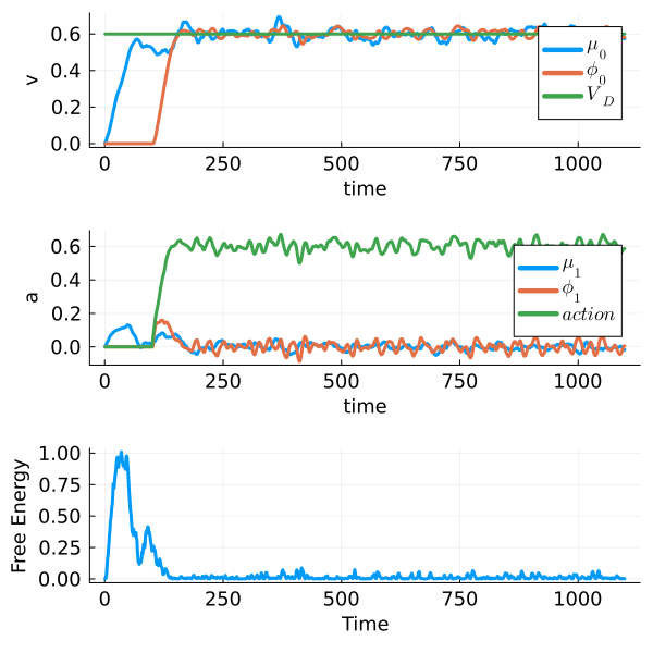
(a)

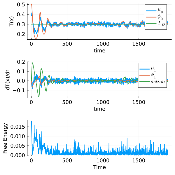
(b)

Figure 6: Two example applications of active inference and the variational free energy principle are shown. In (a), sensory layer spins receive environment position and velocity information and active inference generated by hidden layer spin states drive the system towards a target velocity $v_{d}=0.6$. In (b) environment measures are deterined by a function $T(x)$ and its derivative $dT(x)/dx$, but the sensory spins receive only the values $T$ and $dT/dx$ without information of $x$ or the functional form of $T(x)$. Active inference drives the system to a specified target $T(x)=T_{d}$.

In the above example a model of the environment was encoded in the hidden spin system through $P_{S}$ by inclusion of the dissipation $\alpha$ term. The next and final example illustrates that only the target need be encoded in the hidden states, and additional information can be inferred from the environment at the sensory level.

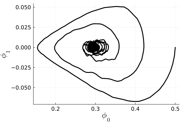
(a)

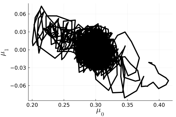
(b)

Figure 7: The trajectory of the sensory spin states is shown in (a) for the example in Fig. 5(b). Active inference feeds information derived from the hidden spin state averages to the environment that causes changes in subsequent sensory input. In this way the trajectory of states within the hidden layer are directed toward the target goal by the sensory spins in response to changes in the environment. The corresponding trajectory for the hidden spins is shown in (b).

The basis of this example is the thermostat problem presented in Buckley [26] and discussed in the context of PID Control by  [28, 31]. The sensory input is from two functions of position $x$ defined by

$$T(x)=\frac{1}{1+x^{2}},$$ (14)

and

$$\frac{d}{dx}T(x)=-\frac{2x}{(1+x^{2})^{2}},,$$ (15)

Action is included in $\frac{dx}{dt}$:

$$\frac{dx(t)}{dt}=a(t),$$ (16)

In this model target information $T_{d}$ is included through $P_{S}(\mu_{1}|T_{d}-\mu_{0})$ but no information about the $\tilde{x}$ is passed to the bilayer. The equations of motion are truncated by requiring $\mu_{3}=0$. Except for the thermal averages over $\chi$, the equations for $\tilde{\mu}$ are of the same form as in  [26]:

$$\frac{d\mu_{0}}{dt}=\mu_{1}+\langle\chi({\beta_{z}(\phi_{0}-\mu_{0}))\rangle_{T}-\langle\chi(\beta_{w}(\mu_{0}+\mu_{1}-T_{d})})\rangle_{T},$$ (17)

$$\frac{d\mu_{1}}{dt}=\mu_{2}+\langle\chi({\beta_{z}(\phi_{1}-\mu_{1}))\rangle_{T}-\langle\chi(\beta_{w}(\mu_{0}+\mu_{1}-T_{d}))\rangle_{T}+\langle\chi(\beta_{w}(\mu_{1}+\mu_{2})})\rangle_{T},$$ (18)

$$\frac{d\mu_{2}}{dt}=-\langle\chi(\beta_{w}(\mu_{1}+\mu_{2}))\rangle_{T}.$$ (19)

The time dependence of the action for this example given by

$$\frac{da}{dt}=-\langle\chi(\beta_{z}(\phi_{1}-\mu_{1}))\rangle_{T}\frac{d}{dx}T(x).$$ (20)

Results are shown in Fig.  6(a) and  6(b) for $T_{s}=0.1$ and $T_{h}=1$ but now with $N_{s}=10$ ($N_{h}$ remains $1$). The increased value of $N_{s}$ helps optimize the trajectory to arrive at the target value $T_{d}=0.3$. The $\mu_{0}$ and $\phi_{0}$ time evolutions are shown in the top panel. The $\mu_{1}$, $\phi_{1}$ and $a$ are shown in the middle panel.

The free energy is shown in the bottom panel and is clearly minimized as the system evolves. The decaying oscillations observed in the $\tilde{\mu_{0}}$ and $\tilde{\phi_{0}}$ are striking and reminiscent of PID as discussed by Balteiri [31]. The authors note that optimization of parameters can be performed to enhance the decay toward the target, as found here also.

It is illuminating to track the evolution through $\phi_{0}$ and $\phi_{1}$ when viewed as a phase space trajectory. The trajectory corresponding to the evolutions of the sensory input in Fig. 7(a) for the time evolution of hidden states shown in Fig. 6(b). The corresponding trajectory for the hidden state $\tilde{\mu}$ is quite different as shown in Fig.  7(b). The sensory inputs circle through $\tilde{\phi}$ to oscillate around the target value. The hidden states $\tilde{\mu}$ evolve quite differently and lie roughly along a quasi-linear line centred about the neighbourhood of the target value. Gradients of the free energy direct evolution of the hidden states towards a most likely peak that lies along this line at the target value. It is useful to note that there is a strong dependence on $N_{s}$ and the system has difficulty finding the target for small values of $N_{s}$ causing it instead to relax to $\phi_{0}=0$.

The optimal parameter values for achieving the target also vary depending on the magnitude of the target $T_{d}$. As noted earlier, thermal evolution during environment time scales within the hidden spin system depend on temperatures and the number of Monte Carlo Steps.

Details of how these parameters affect the trajectories and relaxation are not well understood but some qualitative observations can be reported. The results shown in Figs. 6 and  7 require an amount of environmental time to relax towards the target value and also depend on both $T_{h}$ and $N_{h}$. Increasing $N_{h}$ generally appears to increase the correlation between $\tilde{\mu}$ and $\tilde{\phi}$ while introducing more noise into $\tilde{\mu}$ and the free energy. $T_{h}$ (and its generalization to $\beta_{z}$ and $\beta_{w}$) is an important optimization parameter for achieving the lowest free energy for different $T_{d}$.

A very interesting aspect is the dependence on $\beta_{z}$ and $\beta_{w}$ of the time evolution for $\tilde{\phi}$ and $\tilde{\mu}$. Unusual oscillations can appear for different temperatures and targets that may contain information about internal state selection within the hidden layer. These are aspects currently under study that are outside the scope of the present work, but an example is shown in Fig. 8.

In this figure a target $T_{d}=0.5$ is chosen for $\beta_{z}=3.0$ and $\beta_{w}=0.75$ in Fig. 8(a) and for for $\beta_{z}=2.0$ and $\beta_{w}=0.5$ in Fig. 8(b). In Fig. 8(a) oscillations in $\tilde{\phi}$ and $\tilde{\mu}$ are similar to those shown earlier and are qualitatively the same as what is found using the same values in a gaussian distribution approximation for distributions of $\tilde{\mu}$ states (which is done by replacing the $\langle\chi\rangle_{T}$ with results obtained by assuming gaussian distributions of states as in [26]). The smaller values of $\beta_{z}$ and $\beta_{w}$ used in Fig. 8(b) result in a much different behaviour evidenced by long lived quasi-periodic oscillations. This dependence on temperature and precision weightings suggest that non-trivial dynamics can arise under certain circumstances. This behaviour appears to be sensitive to the geometry of the Artificial Spin Ice. From an experimental perspective, this suggests that active inference might be used to reveal and investigate complex dynamics that can arise in sufficiently complex systems.

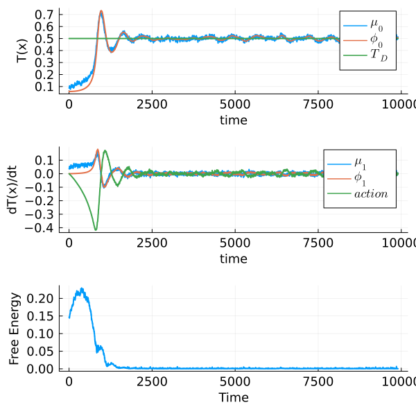
(a)

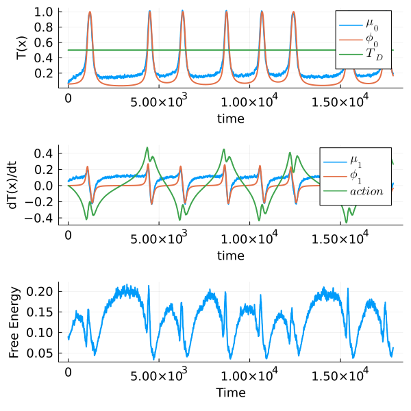
(b)

Figure 8: The oscillations of $\tilde{\mu}$ and $\tilde{\phi}$ relax toward a target $T_{d}=0.5$ in (a) for parameters $\beta_{z}=3.0$ and $\beta_{w}=0.75$. Similar oscillations are found using the same parameters when the $\langle\chi\rangle_{T}$ is replaced with a gaussian distribution approixmation. A very different quasi-periodic oscillation arising from the Artificial Spin Ice through $\langle\chi\rangle_{T}$ is found for $\beta_{z}=2.0$ and $\beta_{w}=0.5$ as shown in (b). A gaussian approximation for these $\beta_{\alpha}$ values is instead similar to the results shown in (a).

V Summary

Perhaps the most interesting aspect demonstrated in this paper is the possibility of studying transition dynamics in other magnetic and nonmagnetic systems using active inference configurations. Viewed as a methodology for probing system dynamics, the mathematical treatment and intrinsic separation of timescales underlying the variational free energy and active inference theory may inspire new ways of experimentally studying a range of complex systems.

The significance of this possibility is that the theory used here can be understood in terms of trajectories of the hidden spinstates which are influenced by constraints imposed dynamically. Essential to this process are the sensory layer spins which provide an interface to the measured environment in a manner analogous to a Markov Blanket as discussed by Kirchhoff, et al. [22]. The mechanisms at play in the spin system involve local fields generated by the sensory spins in response to environment input. The local fields act on the hidden spins, enabling an expedited relaxation towards a minimum free energy defined by a target constraint imposed through active inference. The ability to sample regions of hidden spin state space in this way is reminiscent of, but quite distinct from, other strategies sometimes used for escaping long lived metastable states in computations, such as parallel tempering in studies of spin glasses [32].

It is also interesting to note that the variational Bayes theory used in this paper can be described within a temporally shifted reference frame under the Fokker-Planck Kolmogorov formalism. [33, 27, 34] Together with the use of thermal averaging of the hidden states, this observation suggests that the condition for a stationary trajectory, $\frac{d\mu_{\alpha}}{dt}-D\mu_{\alpha}=0$, in effect matches the environment time scale governing input to the sensory spins with internal hidden state processes that are thermally averaged according to hidden state time scales governing thermal state transitions. As noted by Balaji et al. [29], the stationary trajectory condition means that the hidden spin states evolve along time dependent free energy gradients which lead toward target values. In the simulations discussed in this paper, this condition effectively assigns a physical time interval to thermal transition probabilities sampled using Glauber dynamics. It may be possible to exploit this feature to probe timescales for state transitions processes in experiments for systems whose complex energy landscape is being probed, such as spin or structural glasses.

This connection provides a formalism widely applicable to a variety of systems. Indeed, some work has already appeared in this direction with a suggestion for an active inference interpretation of spin glasses. [35] Trajectories shown in the examples discussed in this paper can be complex, and are sensitive to parameters of the theory that can be interpreted in terms of measurable physical properties. There are some reports in the literature of applications of the free energy principle in physical experiments. One example is saccadic eye motion [2, 36] and another is a recent report for small assemblies of neurons [37]. The purpose of this paper has been to suggest a relatively simple, non-biological system that can also serve as a testing ground for exploring the theory in contexts which can be studied experimentally.

The spin models used throughout this paper are simple yet appear sufficient to capture essential features displayed in experiments using actual nanomagnets. As such, the implementations of active inference suggested here may be possible to observe using suitably designed nanomagnet arrays with fabrication technology that is currently available. This would be interesting for several reasons. The out of equilibrium dynamics illustrated in the two examples described in this paper are interesting in how they emerge from state transitions instigated through application of local fields. The theory of active inference appears to describe well the dynamics observed for averages of the evolving simulated magnetic states. As such, the nanomagnetic geometries proposed here should provide experimentally accessible models. A very interesting next direction to explore would be implementations of hierarchical structures [38] in which multiple sensory and hidden layers could be connected and features associated with learning and other complex tasks explored. Although not reported here, stacked bilayers of the form presented in the present paper appear able to mimic learning processes at different timescales that can facilitate optimizations toward target values.

Concerning possible applications, a great potential of creating energy efficient platforms for machine learning algorithms using nanomagnetic arrays have been identified and some in cases demonstrated [14, 15] as well as other magnetic material platforms. [39, 40]. Most recently, magnetic nanoparticle artificial spin ice configurations have been studied experimentally [16] whose state configurations are manipulated locally and detected using microwaves. The energy efficiency of nanomagnetic systems for machine learning applications, as well as the microwave properties that can be associated with configurational states, make these systems attractive for practicle use. The ability to incorporate active inference in architectures based on nanomagnets would be likewise interesting to pursue.

The nanomagnetic architecture used in this paper is only one example of a nanomagnetic geometry. Although not reported here, some variants of the square ice geometry also display analogous properties under active inference. An advantage to using artificial spin ice as a model platform is the freedom to impose contraints and introduce frustration that can be studied as pathways through configurational states. These can be analysed in a variety of ways including graph theoretical methods as discussed for athermal artificial spin ice by Budrikis [41]. As noted in this work, pathways through state configurations in these systems can often be understood via topological excitations rules associated with their transitions. Active inference methodologies may be helpful in this context to understand how trajectories through configuration space can be manipulated via environmental control of topological excitations.

For this reason it would be particularly exciting to examine in non-Ising spin systems where topological excitations arise through competing interactions. A prime example is magnetic skyrmions in thin film geometries which enable control and detection via local electric potentials. Skyrmions are topologically protected spin textures and display non-linear response to applied fields and undergo transitions through mediating metastable states. [42, 43] These systems can display a sufficiently complex state space for applications in reservoir computing [44, 45].