My Understanding for Static and Dynamic Light Scattering

Abstract

Static Light Scattering (SLS) and Dynamic Light Scattering (DLS) are very important techniques to study the characteristics of nano-particles in dispersion. The data of SLS is determined by the optical characteristic and the measured values of DLS are determined by optical and hydrodynamic characteristics of different size nano-particles in dispersion. Then considering the optical characteristic of nano-particles and using the SLS technique further, the size distribution can be measured accurately and is also consistent with the results measured using the TEM technique. Based on the size distribution obtained using the SLS or TEM technique and the relation between the static and hydrodynamic radii, all the expected and measured values of $g^{\left(2\right)}\left(\tau\right)$ investigated are very well consistent. Since the data measured using the DLS technique contains the information of the optical and hydrodynamic properties of nano-particles together, therefore the accurate size distribution cannot be obtained from the experimental data of $g^{\left(2\right)}\left(\tau\right)$ for an unknown sample. The traditional particle information: apparent hydrodynamic radius and polydispersity index measured using the DLS technique are determined by the optical and hydrodynamic characteristics and size distribution together. They cannot represent a number distribution of nano-particles in dispersion. Using the light scattering technique not only can measure the size distribution accurately but also can provide a method to understand the optical and hydrodynamic characteristics of nano-particles.

1 INTRODUCTION

Light Scattering has been considered to be a well established technique and applied in physics, chemistry, biology, etc. as an essential tool to investigate the characteristics of nano-particles in dispersion. It consists of two parts: Static Light Scattering (SLS) and Dynamic Light Scattering (DLS) techniques. The SLS technique measures the relation between the scattering angles and scattered light intensity and then simplify the relation to the Zimm plot, Berry plot or Guinier plot etc. to get the root mean-square radius of gyration $\left\langle R_{g}^{2}\right\rangle^{1/2}$ and the molar mass of nano-particles provided that the particle sizes are small[1, 2]. The DLS technique has been considered that it can provide a fast and accurate method to measure the particle sizes in dispersion. The apparent hydrodynamic radius and polydispersity index are obtained using the method of Laplace transformation or Cumulant analysis at a given scattering angle[3, 4, 5, 6, 7]. Some researchers believe that the results measured using the SLS and DLS techniques together can be used to obtain much more information of nano-particles [8, 9, 10, 11, 12]. Although the theoretical function of the normalized time electric field auto-correlation function of the scattered light $g^{\left(1\right)}(\tau)$[4, 6, 13] has been proposed, the comparison of the expected values and experimental data of the normalized time auto-correlation function of the scattered light intensity $g^{\left(2\right)}\left(\tau\right)$ has not been detailed and there also exist one assumption that the optical and hydrodynamic radii of nano-particles are same.

For dilute homogeneous spherical particles, one method[15] is proposed to measure the size distribution of nano-particles in dispersion accurately. The size distribution of nano-particles in dispersion is chosen to be a Gaussian distribution. Using a non-linear least square fitting program, the mean static radius $\left\langle R_{s}\right\rangle$ and standard deviation $\sigma$ are measured accurately. Based on our research results, for the polystyrene spherical particles investigated, the size information obtained using the SLS technique and the commercial size information obtained using Transmission Electron Microscopy (TEM) technique provided by the supplier are consistent respectively. They all have a large difference with the corresponding hydrodynamic radii respectively. Using the commercial particle size information, with one assumption, the calculated results and measurements of $g^{\left(2\right)}\left(\tau\right)$ at all the scattering angles investigated are very well consistent. This result also reveals that the static and hydrodynamic radii of spherical nano-particles are different and can have a large difference. For the PNIPAM samples, the fitting results obtained using the non-linear least square fitting program are very well consistent with the data of scattered light intensity and the residuals are random. Based on the static particle size distribution, with one assumption, the calculated results and the measurements of $g^{\left(2\right)}\left(\tau\right)$ at all the scattering angles investigated are also very well consistent. The results also show that the static and hydrodynamic radii of spherical nano-particles are different and can have a much more large difference.

In order to investigate the characteristics of nano-particles in dispersion further, some researchers believe that there exist some relations between the physical quantities obtained using the SLS and DLS techniques. A lot of people believe that the dimensionless shape parameter ${\left\langle{R_{g}}^{2}\right\rangle^{\frac{1}{2}}}/{R_{app,h}}$ can give a good description for the shapes of nano-particles. However based on our analyses, the dimensionless shape parameter is ${\left\langle{R_{g}}^{2}\right\rangle^{\frac{1}{2}}}/{\left\langle{R_{s}}\right\rangle}$. Therefore without the knowledge about the relationship of mean static and apparent hydrodynamic radii, this dimensionless shape parameter ${\left\langle{R_{g}}^{2}\right\rangle^{\frac{1}{2}}}/{R_{app,h}}$ does not make sense.

2 THEORY

For vertically incident polarized light, the average scattered light intensity of a dilute non-interacting particle system in unit volume can be calculated using the following equation for homogeneous spherical particles and when Rayleigh-Gans-Debye(RGD) approximation is valid

$$\frac{I_{s}}{I_{inc}}=\frac{4\pi^{2}\sin^{2}\theta_{1}n_{s}^{2}\left(\frac{dn}{dc}\right)_{c=0}^{2}c}{\lambda^{4}r^{2}}\frac{4\pi\rho}{3}\frac{\int_{0}^{\infty}R_{s}^{6}P\left(q,R_{s}\right)G\left(R_{s}\right)dR_{s}}{\int_{0}^{\infty}R_{s}^{3}G\left(R_{s}\right)dR_{s}},$$ (1)

where $I_{s}$ is the intensity of the scattered light that reaches the detector, $I_{inc}$ is the incident light intensity, $R_{s}$ is the static radius of a particle, $\ q=\frac{4\pi}{\lambda}n_{s}\sin\frac{\theta}{2}$ is the scattering vector, $\lambda$ is the wavelength of incident light in vacuo, $n_{s}$ is the solvent refractive index, $\theta$ is the scattering angle, $\rho$ is the density of particles, $r$ is the distance between the scattering particle and the point of intensity measurement, $c$ is the mass concentration of particles, $\theta_{1}$ is the angle between the polarization of the incident electric field and the propagation direction of the scattered field, $P\left(q,R_{s}\right)$ is the form factor of homogeneous spherical particles

$$P\left(q,R_{s}\right)=\frac{9}{q^{6}R_{s}^{6}}\left(\sin\left(qR_{s}\right)-qR_{s}\cos\left(qR_{s}\right)\right)^{2}$$ (2)

and $G\left(R_{s}\right)$ is the number distribution of particles in dispersion and is chosen as a Gaussian distribution

$$G\left(R_{s};\left\langle R_{s}\right\rangle,\sigma\right)=\frac{1}{\sigma\sqrt{2\pi}}\exp\left(-\frac{1}{2}\left(\frac{R_{s}-\left\langle R_{s}\right\rangle}{\sigma}\right)^{2}\right),$$ (3)

where $\left\langle R_{s}\right\rangle$ is the mean static radius and $\sigma$ is the standard deviation.

Based on the particle size information obtained using the SLS technique, for dilute homogeneous spherical particles, $g^{\left(1\right)}(\tau)$ is

$$g^{\left(1\right)}\left(\tau\right)=\frac{\int R_{s}^{6}P\left(q,R_{s}\right)G\left(R_{s}\right)\exp\left(-q^{2}D\tau\right)dR_{s}}{\int R_{s}^{6}P\left(q,R_{s}\right)G\left(R_{s}\right)dR_{s}},$$ (4)

where $D$ is the diffusion coefficient.

Here the Stokes-Einstein relation[16] is still considered to be true for nano-particles in dispersion,

$$D=\frac{k_{B}T}{6\pi\eta_{0}R_{h}},$$ (5)

where $\eta_{0}$, $k_{B}$ and $T$ are the viscosity of solvent, Boltzmann’s constant and absolute temperature respectively, then the hydrodynamic radius $R_{h}$ can be obtained.

The relation between the static and hydrodynamic radii in this work is assumed to be

$$R_{h}=kR_{s},$$ (6)

where $k$ is a constant. Based on the Siegert relation between $g^{\left(2\right)}\left(\tau\right)$ and $g^{\left(1\right)}\left(\tau\right)$ [7]

$$g^{\left(2\right)}\left(\tau\right)=1+\beta\left(g^{\left(1\right)}\right)^{2},$$ (7)

the function between the SLS and DLS techniques is built and the values of $g^{\left(2\right)}\left(\tau\right)$ can be expected based on the particle size information measured using the SLS technique.

3 TRADITIONAL ANALYSIS

In general, Static Light Scattering is a technique that can used to measure the root mean square radius or radius of gyration $\left\langle R_{g}^{2}\right\rangle^{1/2}$ in dispersion by measuring the scattered light intensity at many scattering angles. The values can be obtained using the following Zimm plot analysis.

$$Kc/R_{vv}=1/M(1+q^{2}\left\langle R_{g}^{2}\right\rangle/3)$$ (8)

where $R_{vv}$ is the Rayleigh ratio $r^{2}I_{s}/I_{inc}$, $\left\langle R_{g}^{2}\right\rangle^{1/2}$ is the radius of gyration.

Traditionally for non-interacting mono-disperse nano-particles in dispersion, $g^{\left(1\right)}\left(\tau\right)$ can be written as

$$g^{\left(1\right)}\left(\tau\right)=exp{\left(-\Gamma\tau\right)}$$ (9)

where $\Gamma=q^{2}D$ is the decay rate, $D$ represents the macromolecular translational diffusion coefficient of the particles.

For a polydisperse system, $g^{\left(1\right)}\left(\tau\right)$ can be written as

$$g^{\left(1\right)}\left(\tau\right)=\int{G{\left(\Gamma\right)}exp{\left(-\Gamma\tau\right)}d\Gamma}$$ (10)

where $G{\left(\Gamma\right)}$ is the normalized distribution of the decay rates.

The size distribution can be obtained using the method of moment analysis. The mean decay rate $\overline{\Gamma}$ and the moments of the distribution $\mu_{2}$ are defined as

$$\overline{\Gamma}=\int{\Gamma G{\left(\Gamma\right)}d\Gamma}$$ (11)

$$\mu_{2}=\int{{\left(\Gamma-\overline{\Gamma}\right)}^{2}G{\left(\Gamma\right)}d\Gamma}$$ (12)

Based on the Stokes-Einstein relation, an apparent hydrodynamic radius $R_{app,h}$ can be defined as

$$D=\frac{k_{B}T}{6\pi\eta_{0}R_{app,h}}=\overline{\Gamma}/q^{2},$$ (13)

The polydispersity index also can be defined as

$$PD.I=\frac{\mu_{2}}{{\overline{\Gamma}}^{2}}.$$ (14)

However the relation between the polydispersity index, apparent hydrodynamic radius $R_{app,h}$ and the particle size distribution does not be detailed.

The dimensionless shape parameter $\rho$ is defined as

$$\rho={\left\langle{R_{g}}^{2}\right\rangle^{\frac{1}{2}}}/{R_{app,h}}$$ (15)

are used to infer particle shapes. However based on the definition of the root mean-square radius of gyration $\left\langle R_{g}^{2}\right\rangle^{1/2}$, the definition $\rho$ is

$$\rho={\left\langle{R_{g}}^{2}\right\rangle^{\frac{1}{2}}}/{\left\langle R_{s}\right\rangle}$$ (16)

4 RESULTS AND DISCUSSION

4.1 Standard polystyrene latex samples

The commercial particle size information was measured by using the TEM technique provided by the supplier. Since there exists a large difference between the refractive indices of the polystyrene latex (1.591 at wavelength 590 nm and 20 ^oC) and water (1.332), i.e., the “phase shift” $\frac{4\pi}{\lambda}R|m-1|$ [6, 14] of Latex-1 and Latex-2 are 0.13 and 0.21 respectively. They do not exactly satisfy the rough criterion that a RGD approximation[6] is valid. Therefore the mono-disperse model $G\left(R_{s}\right)=\delta\left(R_{s}-\left\langle R_{s}\right\rangle\right)$ was used to obtain the values of $\left\langle R_{s}\right\rangle$. All the results measured using the SLS technique and TEM are listed in Table 1. The fitting results and measured data are shown in Figs. 4.1a and 4.1b, respectively. The results reveal that the values measured using the SLS and TEM techniques are very well consistent.

$\left\langle R\right\rangle_{comm}$ (nm)	$\sigma_{comm}$ (nm)	$\left\langle R_{s}\right\rangle$ (nm)
33.5(Latex-1)	2.5	33.3$\pm$0.2
55(Latex-2)	2.5	56.77$\pm$0.04

Table 1: Size information measured using the TEM and SLS techniques.

$\begin{array}[]{c@{\hspace{0in}}c}\includegraphics[width=145.99367pt,angle={-90}]{Poly33cal.eps}&\includegraphics[width=145.99367pt,angle={-90}]{Poly55fit.eps}\\[0.0pt] \end{array}$

Figure 1: a). The experimental data and fitting results of $I_{s}/I_{inc}$ for Latex-1 and b). Latex-2. The circles show the experimental data and the line represents the fitting results of $I_{s}/I_{inc}$.

Since the size information measured using the SLS and TEM techniques are consistent, so the particle size information provided by the supplier are used to calculate the expected values of $g^{\left(2\right)}\left(\tau\right)$. In these calculations, the constant $k$ in Eq. 6 is set to be 1.1 for Latex-1 and 1.2 for Latex-2. Figs. 4.1a and 4.1b show all the experimental data and expected values of $g^{\left(2\right)}\left(\tau\right)$ at the scattering angles 30^o, 60^o, 90^o, 120^o and 150^o and a temperature of 298.45 K for Latex-1, 298.17 K for Latex-2 respectively. Figure 4.1 shows that the experimental data and expected values are very well consistent.

$\begin{array}[]{c@{\hspace{0in}}c}\includegraphics[width=145.99367pt,angle={-90}]{Poly33DLScal.eps}&\includegraphics[width=145.99367pt,angle={-90}]{Poly55DLScal.eps}\\[0.0pt] \end{array}$

Figure 2: The experimental data and expected values of $g^{\left(2\right)}\left(\tau\right)$. a). Latex-1 and b). Latex-2. The symbols represent the experimental data and the lines show the expected values calculated under $R_{h}=kR_{s}$.

4.2 PNIPAM samples

When the data of the PNIPAM-1 measured using the SLS technique at a temperature of 302.33 K was fitted using Eq. 1, the fitting results show that if a small scattering vector range is chosen, the parameters are not well-determined. The uncertainties in the parameters will decrease and $\left\langle R_{s}\right\rangle$ and $\sigma$ stabilize if the scattering vector range is increased. As the scattering vector range continues to increase, the values of $\left\langle R_{s}\right\rangle$ and $\sigma$ begin to lose stability and $\chi^{2}$ grows as shown in Table 4.2. Therefore the stable fitting results $\left\langle R_{s}\right\rangle=254.3\pm 0.1$ nm and $\sigma=21.5\pm 0.3$ nm obtained in the scattering vector range between 0.00345 and 0.01517 nm^-1 are chosen as the particle size information measured using the SLS technique. All the experimental data, stable fitting results and residuals in the scattering vector range between 0.00345 and 0.01517 nm^-1 are shown in Fig. 4.2. The figure reveals that the fitting results and measured data are very well consistent and the residuals are random.

$q$ ($10^{-3}$ nm-1)	$\left\langle R_{s}\right\rangle$ (nm)	$\sigma$ (nm)	$\chi^{2}$
3.45 to 9.05	260.09$\pm$9.81	12.66$\pm$19.81	1.64
3.45 to 11.18	260.30$\pm$1.49	12.30$\pm$3.37	1.65
3.45 to 13.23	253.45$\pm$0.69	22.80$\pm$0.94	2.26
3.45 to 14.21	254.10$\pm$0.15	21.94$\pm$0.36	2.03
3.45 to 15.17	254.34$\pm$0.12	21.47$\pm$0.33	2.15
3.45 to 17.00	255.40$\pm$0.10	17.32$\pm$0.22	11.02

Table 2: The results obtained using Eq. 1 for PNIPAM-1 at different scattering vector ranges and a temperature of 302.33 K.

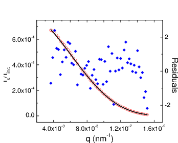
Figure 3: The experimental data and stable fitting results for PNIPAM-1 at a temperature of 302.33 K. The circles show the experimental data, the line shows the fitting results and the diamonds show the residuals: $\left(y_{i}-y_{fit}\right)/\sigma_{i}$.

Based on the particle size information measured using the SLS technique with the constant $k=1.21$ in Eq. 6, the expected values of $g^{\left(2\right)}\left(\tau\right)$ at the scattering angles 30^o, 50^o and 70^o are calculated. All the measured data and expected values are shown in Fig. 4.2. Figure 4.2 reveals that the expected values and experimental data are very well consistent.

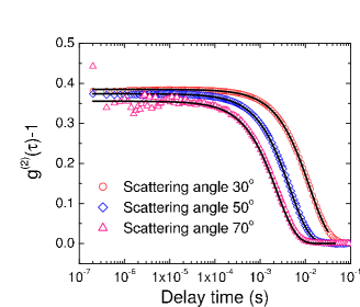
Figure 4: The measured data and expected values of $g^{\left(2\right)}\left(\tau\right)$ of PNIPAM-1 at a temperature of 302.33 K. The symbols represent the experimental data and the lines show the expected values calculated under $R_{h}=1.21R_{s}$.

When the PNIPAM samples in dispersion are at high temperatures, all the situations that fit using Eq. 1 are the same as that of PNIPAM-1 at a temperature of 302.33 K. The fitting values of $\left\langle R_{s}\right\rangle$ and $\sigma$ are affected by a scattering vector range. The uncertainties in the parameters will decrease and $\left\langle R_{s}\right\rangle$ and $\sigma$ stabilize if the scattering vector range is increased. For PNIPAM-5 at a temperature of 312.66 K, the stable fitting results $\left\langle R_{s}\right\rangle=139.3\pm 0.3$ nm and $\sigma=12.4\pm 0.6$ nm obtained in the scattering vector range between 0.00345 and 0.02555 nm^-1 are chosen as the particle size information measured using the SLS technique. The stable fitting results and residuals are shown in Figure 4.2a. With the constant $k=1.1$ in Eq. 6, the expected values of $g^{\left(2\right)}\left(\tau\right)$ at the scattering angles 30^o, 50^o, 70^o and 100^o are calculated. All the experimental and expected values are shown in Fig. 4.2b. The expected values and measured data of $g^{\left(2\right)}\left(\tau\right)$ also are very well consistent.

$\begin{array}[]{c@{\hspace{0in}}c}\includegraphics[width=145.99367pt,angle={-90}]{PNIhTfit.eps}&\includegraphics[width=145.99367pt,angle={-90}]{PNIhTcal.eps}\\[0.0pt] \end{array}$

Figure 5: The static and dynamic results of PNIPAM-5 at a temperature 312.66 K. a). The measured data and stable fitting results. The circles represent the experimental data, the line shows the fitting results and the diamonds represent the residuals: $\left(y_{i}-y_{fit}\right)/\sigma_{i}$. b). The measured data and expected values of $g^{\left(2\right)}\left(\tau\right)$. The symbols represent the measured data and the lines show the expected values calculated under $R_{h}=1.1R_{s}$.

For all other samples investigated, the same situation has been obtained. The fitting results of $\left\langle R_{s}\right\rangle$ and $\sigma$ are affected by a scattering vector range. If a small scattering vector range is used, the parameters are not well-determined. The uncertainties in the parameters will decrease and $\left\langle R_{s}\right\rangle$ and $\sigma$ stabilize if the scattering vector range is increased. The expected values of $g^{\left(2\right)}\left(\tau\right)$ calculated based on the particle size distribution measured using the SLS technique or commercial results provided by the supplier and measured data are very well consistent. All the results reveal that the static radius of nano-particles in dispersion can have a very large difference with hydrodynamic radius.

For the DLS technique, two important parameters that people try to measure accurately from the DLS data are an apparent hydrodynamic radius and polydispersity index. People also believe that the values of polydispersity index represent the size distribution of nano-particles. The small values mean the size distribution is narrow or mono-disperse then the apparent hydrodynamic radius will be equal to the mean hydrodynamic radius. Since the apparent hydrodynamic radius and polydispersity index of nano-particles are measured from the non-exponentility of the correlation function of temporal fluctuation in the scattered light at a given scattering angle, therefore the effects of nano-particle size distribution and scattering angles on the correlation function of temporal fluctuation in the scattered light were investigated further. For simplicity, let $k=1$ that means the values of the static and hydrodynamic radii of homogeneous spherical particles are same.

Using the Cumulant method at a given scatter angle $q$ as $\tau\rightarrow 0$, the equations of the apparent hydrodynamic radius ${R_{app,h}}$ and polydispersity index $PD.I$ are

$${R_{app,h}}=\frac{\int_{0}^{\infty}R_{s}^{6}P\left(q,R_{s}\right)G\left(R_{s}\right)dR_{s}}{\int_{0}^{\infty}R_{s}^{5}P\left(q,R_{s}\right)G\left(R_{s}\right)dR_{s}}$$ (17)

and

$$PD.I=\frac{\int_{0}^{\infty}R_{s}^{4}P\left(q,R_{s}\right)G\left(R_{s}\right)dR_{s}\int_{0}^{\infty}R_{s}^{6}P\left(q,R_{s}\right)G\left(R_{s}\right)dR_{s}}{\left(\int_{0}^{\infty}R_{s}^{5}P\left(q,R_{s}\right)G\left(R_{s}\right)dR_{s}\right)^{2}}-1.$$ (18)

The expected values of ${R_{app,h}}$ and $PD.I$ were calculated for the mean hydrodynamic radius 5 nm and different standard deviations at scattering angles 0^o, 30^o, 60^o, 90^o and 120^o. All the results are shown in Figs. 4.2a and 4.2b, respectively. During the process, the wavelength of the incident light in vacuo $\lambda$ is set to 632.8 nm and solvent refractive index $n_{s}$ is 1.332.

$\begin{array}[]{c@{\hspace{0in}}c}\includegraphics[width=145.99367pt,angle={-90}]{RhRadiusS.eps}&\includegraphics[width=145.99367pt,angle={-90}]{PDIS.eps}\\[0.0pt] \end{array}$

Figure 6: a). The apparent hydrodynamic radius and b). polydispersity index as a function of relative standard deviation at different scattering angles with mean hydrodynamic radius 5 nm.

Figure 4.2a reveals that the effects of the relative standard deviation on the apparent hydrodynamic radius is huge. Figure 4.2b shows that polydispersity index always is small and increase to about 0.1 as the values of relative standard deviation change to very large.

Next the situation of large particles also was investigated. The mean hydrodynamic radius is 100nm. The expected values of ${R_{app,h}}$ and $PD.I$ were calculated as a function of relative standard deviation at scattering angles 0^o, 30^o, 60^o, 90^o and 120^o. The results are shown in Figs. 4.2a and 4.2b, respectively. Figure 4.2a and 4.2b reveal that the effects of the relative standard deviation and scattering angles on the apparent hydrodynamic radius and polydispersity index are huge and complex.

Based on the discussion above, even if the value of polydispersity index is small and the values of apparent hydrodynamic radii measured are consistent at different scattering angles for an unknown sample, the conclusion that the particle size distribution is narrow or mono-disperse still cannot be obtained.

$\begin{array}[]{c@{\hspace{0in}}c}\includegraphics[width=145.99367pt,angle={-90}]{RhRadiusL.eps}&\includegraphics[width=145.99367pt,angle={-90}]{PDIL.eps}\\[0.0pt] \end{array}$

Figure 7: a). The apparent hydrodynamic radius and b). polydispersity index as a function of relative standard deviation at scattering angles 0^o, 30^o, 60^o, 90^o and 120^o for the nanoparticles with mean hydrodynamic radius 100 nm.

For the polystyrene latex samples investigated, the results obtained using the TEM, SLS and DLS techniques are listed in Table 4.2.

$R_{TEM}$(nm)	$\left\langle R_{s}\right\rangle$(nm)	$R_{app,h}$ (nm)	$R_{app,h}/\left\langle R_{s}\right\rangle$
33.5	33.3$\pm$0.2	37.27$\pm$0.09	1.119$\pm$0.007
55	56.77$\pm$0.04	64.5$\pm$0.6	1.14$\pm$0.01
90	92.05$\pm$0.04	103.1$\pm$0.4	1.120$\pm$0.004

Table 3: Commercial $R_{TEM}$, $\left\langle R_{s}\right\rangle$ and apparent hydrodynamic radii.

The results above reveal that the sizes obtained using the SLS and TEM techniques are very well consistent. Even for very narrow samples, the value of the apparent hydrodynamic radius obtained under the same conditions as the static radius is larger than that of the static radius by about $12\%$.

Meanwhile the values of the root mean square radius of gyration ${\left\langle{R_{g}}^{2}\right\rangle}^{1/2}$ also can be calculated using the commercial size distribution. The expected and measured values obtained from the Zimm plot analysis are listed in Table 4.2. All the results reveal that particle size information measured using the SLS and TEM are consistent.

Sample	${\left\langle{R_{g}}^{2}\right\rangle}^{1/2}_{cal}$	${\left\langle{R_{g}}^{2}\right\rangle}^{1/2}_{Zimm}$
33.5(nm)	26.9	26.9$\pm$0.5
55 (nm)	43.24	46.8$\pm$0.3
90 (nm)	70.1	69.0$\pm$2.0

Table 4: Values of ${\left\langle{R_{g}}^{2}\right\rangle}^{1/2}_{cal}$ and ${\left\langle{R_{g}}^{2}\right\rangle}^{1/2}_{Zimm}$.

For the PNIPAM samples investigated, the dimensionless parameters of $\rho$, ${\left\langle{R_{g}}^{2}\right\rangle}^{1/2}_{Zimm}/\left\langle R_{s}\right\rangle$ and ${\left\langle{R_{g}}^{2}\right\rangle}^{1/2}_{cal}/\left\langle R_{s}\right\rangle$ also have been measured or calculated respectively. All the results are shown in Table 4.2. All the results also reveal that the particle size information obtained using the SLS technique is more accurate to represent the particle information in dispersion. The dimensionless parameter $\rho$ cannot give a good description for the shapes of nano-particles in dispersion.

Sample (Temperature)	$\rho$	${\left\langle{R_{g}}^{2}\right\rangle}^{1/2}_{Zimm}/\left\langle R_{s}\right\rangle$	${\left\langle{R_{g}}^{2}\right\rangle}^{1/2}_{cal}/\left\langle R_{s}\right\rangle$
PNIPAM-5($40^{o}$C)	0.73$\pm$0.02	0.83$\pm$0.03	0.813$\pm$0.003
PNIPAM-2($40^{o}$C)	0.69$\pm$0.03	0.84$\pm$0.04	0.82$\pm$0.01
PNIPAM-1($40^{o}$C)	0.69$\pm$0.03	0.87$\pm$0.04	0.856$\pm$0.009
PNIPAM-0($40^{o}$C)	0.66$\pm$0.01	0.80$\pm$0.02	0.81$\pm$0.01
PNIPAM-0($34^{o}$C)	0.54$\pm$0.02	1.13$\pm$0.03	1.04$\pm$0.03

Table 5: Values of the dimensionless parameters of $\rho$, ${\left\langle{R_{g}}^{2}\right\rangle}^{1/2}_{Zimm}/\left\langle R_{s}\right\rangle$ and ${\left\langle{R_{g}}^{2}\right\rangle}^{1/2}_{cal}/\left\langle R_{s}\right\rangle$.

Based on the discussion above, the size distribution obtained using the SLS technique is consistent with that measured using the TEM technique and can be more accurate to represent the size distribution of nano-particles in dispersion. The data of $g^{\left(2\right)}\left(\tau\right)$ measured using the DLS technique are determined by the optical and hydrodynamic properties and size distribution of nano-particles in dispersion together. Therefore the apparent hydrodynamic radius (optical weight hydrodynamic radius) can have a large difference with the corresponding mean static radius and the ratio of $R_{app,h}/\left\langle R_{s}\right\rangle$ can be larger than 2.

5 CONCLUSION

Eq. 1 provides a new method to measure the size distribution of nano-particles in dispersion using the SLS technique. The size distributions of polystyrene latex samples obtained using the TEM and SLS techniques are consistent to reveal that the static size distribution is corresponding to the ordinary number particle size distribution. Using the SLS technique to study the scattered light of different shape nano-particles in dispersion further not only can measure the size distribution of nano-particles accurately but also can provide a method to understand the light scattering characteristics based on the knowledge of the structure of nano-particles in dispersion.

The data of $g^{\left(2\right)}\left(\tau\right)$ measured using the DLS technique contains the information of the optical and hydrodynamic properties of nano-particles together and can be affected largely by the size distribution, therefore the accurate size distribution cannot be obtained from the experimental data of $g^{\left(2\right)}\left(\tau\right)$ for an unknown sample. However based on the particle size information obtained using the SLS technique, a possible way to explore the hydrodynamic characteristics of nano-particles in dispersion further is provided.

References

- [1] Zimm B H 1948 J. Chem. Phys. 16 1099.
- [2] Burchard W 1983 Adv. Polym. Sci. 48 1.
- [3] Koppel D E 1972 J. Chem. Phys. 57 4814.
- [4] Bargeron C B 1974 J. Chem. Phys. 61 2134.
- [5] Brown J C, Pusey P N and Dietz R 1975 J. Chem. Phys. 62 1136.
- [6] Berne B J and Pecora R Dynamic Light Scattering (Robert E. Krieger Publishing Company, Malabar, Florida, 1990).
- [7] Brown W Dynamic Light Scattering: The Method and Some Applications (Clarendon Press, Oxford, 1993).
- [8] Bryant G, Martin S, Budi A and van Megen W 2003 Langmuir 19 616.
- [9] Burchard W, Kajiwara K and Nerger D 1982 J. Polym. Sci. 20 157
- [10] Burchard W, Schmidt M and Stockmayer W H 1980 Macromolecules 13 1265.
- [11] Hu T and Wu C 1999 Phys. Rev. Lett. 83 4105.
- [12] Wu J, Huang G and Hu Z 2003 Macromolecules 36 440.
- [13] Pusey P N and van Megen W 1984 J. Chem. Phys. 80 3513.
- [14] van de Hulst H C Light Scattering by Small Particles (Dover Publications, Inc. New York, 1981).
- [15] Sun Y C Different Particle Size Information Obtained From Static and Dynamic Laser Light Scattering (Thesis, Simon Fraser University, 2004).
- [16] The ALV Manual of the version for ALV-5000/E for Windows, ALV-Gmbh, Germany, 1998.