On the Evolution During Growth of Regular Boundaries of Bodies into Fractals

Abstract.

Generalizing smooth volumetric growth to the singular case, using de Rham currents and flat chains, we demonstrate how regular boundaries of bodies may evolve to fractals.

1. Introduction

Fractals are limiting geometric objects obtained by rescaling an initial object for scales that tend to zero. A fractal can be constructed by geometric iterations as a complex invariant object from the solution of a dynamical system (so-called a strange attractor) that is usually studied by probabilistic methods.

Fractal boundaries of domains in $\mathbb{R}^{n}$ can have a dimension that is larger than $n-1$. More precisely, the Hausdorff dimension of a fractal boundary can be any number between $n$ and $n-1$. The rate of growth of the measure of the fractal boundary during its construction by iterations or its evolution in time, depends directly on its Hausdorff dimension. For example, the Hausdorff dimension of the boundary of the classical von Koch snowflake is $\ln 4/\ln 3$.

Fractals often serve as mathematical models for complex geometries. While models of physical and biological systems may not apply at arbitrarily small scales, modeling such systems by fractals provides a convenient framework and obviates the need to specify the range of scales where the geometric model applies.

Growth processes sometimes exhibit fractal-like behavior. The growth patterns during phase transition (see, e.g., [Suz83, SC89]), growth patterns in trees, [Bar88], and growth of bacterial colonies, e.g., [FM89, OPS90, FM91] (see Figure 1.1), provide examples of such processes. Fractal-like boundaries imply larger a surface area relative to the volume for the transport of nutrients.

The mechanics of growth from the point of view of continuum mechanics has gained attention since the end of the 20th century (see [SDM⁺82, Tab95, SE96]). Growth and the possible creation and destruction of body points seem to contradict the principle of material impenetrability of continuum mechanics.

Surface growth, an important mode of growth, and its consequences in terms of stresses and forces (for example, loc. cit, [SY16, TZ19, PY23]), offers a particular challenge in the study of continuum theories of growth. While theories of surface growth usually consider the evolution of smooth surfaces, this paper considers the evolution of fractal-like surfaces, specifically, the evolution of polyhedral and smooth surfaces to fractals.

In this paper, some fractals are modeled mathematically as de Rham currents. This is a natural extension of smooth volumetric growth to the singular case. In the general formulation, this setting applies in the general framework of proto-Galilean spacetime, a general fiber bundle over the time axis (see [SE22, GS23]). As a typical example, we consider the von Koch snowflake, modeled by a flat chain as in Whitney’s geometric integration theory, [Whi57].

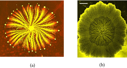
Figure 1.1. Fractal-like bacteria colonies:
(a) Paenibacillus vortex sp. bacteria. (By Eshel Ben-Jacob, https://commons.wikimedia.org/wiki/File: 
Paenibacillus_vortex_colony.jpg.)
(b) Surface morphologies of 14 days old WT Bacillus subtilis biofilm. Taken from [WBFW22] with permission of the authors.

As background, we review in Section 2 the basic notions of smooth flux theory and volumetric growth in a proto-Galilean spacetime, as in [GS23]. Special attention is given to the role played by a frame, a trivialization, as opposed to frame invariant variables and operations. The theory is extended to the singular case in Section 3 using the theory of de Rham currents. We briefly review the basic notions of de Rham currents, propose the relevant generalization of smooth volumetric growth to the singular case, and give the example of surface growth as singular volumetric growth.

Whitney’s geometric integration theory for flat chains [Whi57] may be presented as a special case of the theory of currents, as in [Fed69]. We present the fundamental ideas in Section 4. Flat chains may be used to model various fractals, and we outline the construction of the von Koch snowflake as an example.

The continuous evolution of a polyhedron to a fractal, the snowflake, is demonstrated in Section 5.

Finally, in Section 5, we use the theory of conformal mappings and prime ends to propose a construction of a smooth evolution of a two-dimensional region having a smooth boundary into a fractal.

2. Smooth Growth in a Proto-Galilean Spacetime

This section describes the geometric setting of spacetime for what follows and presents the basic objects used to describe mathematically smooth volumetric growth. In our formulation, smooth volumetric growth arise from a nonvanishing source of an extensive property, mass, for example. Body points corresponding to the extensive property under consideration, may be defined. Since one considers time-evolution of the extensive property, a specific model of spacetime should be used.

2.1. Proto-Galilean spacetime

We use a generalized model of Galilean spacetime, proto-Galilean spacetime (see [SE22]). It is classical in the sense that to each event $e$ there corresponds a unique time $t=\pi(e)$. Thus, if $\mathcal{E}$ denotes spacetime, and taking the time axis as $\mathbb{R}$ for the sake of simplicity, there is a mapping

$$\pi:\mathcal{E}\longrightarrow\mathbb{R}.$$ (2.1)

For each time $t\in\mathbb{R}$, the inverse image $\mathcal{E}_{t}:=\pi^{-1}\{t\}$, the collection of simultaneous events at $t$, is assumed to be diffeomorphic with an $n$-dimensional space oriented manifold $\mathcal{S}$. However, in accordance with the Galilean point of view that location in space is not absolute, there is no unique oriented preserving diffeomorphism

$$\Phi_{t}:\mathcal{E}_{t}\longrightarrow\mathcal{S}.$$ (2.2)

Spacetime $\mathcal{E}$ is assumed to be an $(n+1)$-dimensional manifold having a fiber bundle structure provided by a collection of (local) frames $\{(U_{a},\Phi_{a})\}$, such that the collection $\{U_{a}\}$ is an open cover of $\mathbb{R}$ and

$$\Phi_{a}:\pi^{-1}(U_{\alpha})\longrightarrow U_{a}\times\mathcal{S},\qquad\text{such that}\qquad\textrm{pr}_{1}\circ\Phi_{a}=\pi$$ (2.3)

are diffeomorphisms. Here, $\textrm{pr}_{1}$ and $\textrm{pr}_{2}$ denote the projections on the first and second factors of the Cartesian product, respectively. Thus, simply, a frame associates a particular point $x\in\mathcal{S}$ with each event $e$, and

$$\Phi_{a}:e\longmapsto(t,x).$$ (2.4)

Given, another frame,

$$\Phi_{b}:\pi^{-1}(U_{b})\longrightarrow U_{b}\times\mathcal{S},\qquad e\longmapsto(t^{\prime}=t,x^{\prime})$$ (2.5)

such that $U_{a}\cap V_{b}\neq\varnothing$, $t\in U_{a}\cap V_{b}$, there is a transformation

$$\Phi_{ba}(t):=\Phi_{b}\circ\Phi_{a}^{-1}|_{t}:\mathcal{S}\longrightarrow\mathcal{S},\qquad x\longmapsto x^{\prime}.$$ (2.6)

If $x^{i}$ are coordinates in a neighborhood of $x$, and $x^{\prime j}$ are coordinates in a neighborhood of $x^{\prime}$, the mapping $\Phi_{ba}$ is represented by functions

$$x^{\prime j}=x^{\prime j}(t,x^{i}).$$ (2.7)

The tangent mapping of the time-projection is

$$T\pi:T\mathcal{E}\longrightarrow T\mathbb{R}.$$ (2.8)

Let $\boldsymbol{1}$be the natural tangent base vector to the time axis and let $\boldsymbol{1}^{*}$ be the dual element of $T^{*}\mathbb{R}$. Then, a natural one form $\textrm{d}t$ is induced in spacetime by the pullback of forms as

$$\textrm{d}t=T^{*}\pi(\boldsymbol{1}^{*}).$$ (2.9)

Evidently, $\textrm{d}t$ is frame-independent.

Another frame-independent notion is that of a spacelike tangent vector. A vector $v\in T\mathcal{E}$ is said to be spacelike if it is vertical, that is, if

$$T\pi(v)=0.$$ (2.10)

Note that if $v$ is spacelike,

$$\begin{split}\textrm{d}t(v)&=T^{*}\pi(\boldsymbol{1}^{*})(v),\\ &=\boldsymbol{1}^{*}(T\pi(v)),\\ &=0.\end{split}$$ (2.11)

Conversely, if $\textrm{d}t(v)=0$, $v$ is spacelike. The collection of spacelike tangent vectors, an $n$-dimensional subbundle of $T\mathcal{E}$ will be denoted as $V\mathcal{E}$. With some abuse of notation, we write

$$\tau:V\mathcal{E}\longrightarrow\mathcal{E},$$ (2.12)

for the restriction of

$$\tau:T\mathcal{E}\longrightarrow\mathcal{E},$$ (2.13)

and we write

$$\mathcal{I}_{V}:V\mathcal{E}\longrightarrow T\mathcal{E}$$ (2.14)

for the inclusion mapping of the subbundle.

For any time $t\in\mathbb{R}$, a spacelike vector is tangent to the $\mathcal{E}_{t}$ and the vector bundle $(V\mathcal{E})_{t}$ is identical to $T(\mathcal{E}_{t})$

 

We now consider additional objects available once a frame, $\Phi$, on spacetime is given. To simplify the notation, we write the expressions for the case where the frame is global in the sense that its domain is $\mathcal{E}$. The tangent mapping

$$T\Phi:T\mathcal{E}\longrightarrow T(\mathbb{R}\times\mathcal{S})=T\mathbb{R}\times T\mathcal{S}$$ (2.15)

is a vector bundle isomorphism. The components of $T\Phi$, are

$$T\Phi_{1}:T\mathcal{E}\longrightarrow T\mathbb{R},\quad v\longmapsto v^{t},\quad\text{and}\quad T\Phi_{2}:T\mathcal{E}\longrightarrow T\mathcal{S},\quad v\longmapsto v_{x}.$$ (2.16)

Thus, we may define the vector field

$$\partial_{t}=\frac{\partial}{\partial t}:=T\Phi^{-1}(\boldsymbol{1},0).$$ (2.17)

It is emphasized that the “timelike” unit vector $\partial_{t}$ is frame-dependent as it requires one to keep the location in space “fixed” for distinct times. Note that

$$\begin{split}\textrm{d}t(\partial_{t})&=T^{*}\pi(\boldsymbol{1}^{*})(T\Phi^{-1}(\boldsymbol{1},0)),\\ &=\boldsymbol{1}^{*}(T\pi\circ T\Phi^{-1}(\boldsymbol{1},0)),\\ &=\boldsymbol{1}^{*}(T(\pi\circ\Phi^{-1})(\boldsymbol{1},0)),\\ &=\boldsymbol{1}^{*}(T\textrm{pr}_{1}(\boldsymbol{1},0)),\\ &=\boldsymbol{1}^{*}(\boldsymbol{1}),\end{split}$$ (2.18)

where in the fourth line we used (2.3), which implies

$$\begin{split}\pi\circ\Phi^{-1}&=\textrm{pr}_{1}\circ\Phi\circ\Phi^{-1},\\ &=\textrm{pr}_{1}\end{split}$$ (2.19)

Thus, while $\partial_{t}$ depends on the frame,

$$\textrm{d}t(\partial_{t})=1$$ (2.20)

independently of the frame. This also implies that $\partial_{t}$ is not spacelike, and that it complements the vertical subbundle to the tangent bundle $T\mathcal{E}$.

In addition, it follows from (2.3) that for any $v\in T\mathcal{E}$, we have,

$$T\pi(v)=T(\textrm{pr}_{1}\circ\Phi)(v)=T\textrm{pr}_{1}\circ T\Phi(v),$$ (2.21)

thus, $v$ is vertical if and only if

$$v^{t}=T\Phi_{1}(v)=0.$$ (2.22)

We conclude that every vector $v\in T\mathcal{E}$ is represented locally as

$$v=v^{t}\partial_{t}+v_{x}^{i}\partial_{i},$$ (2.23)

and every vertical vector is of the local form

$$v=v_{x}^{i}\partial_{i}.$$ (2.24)

Let $\Phi^{\prime}$ be another frame so that the transformation rule is represented locally as in (2.7),

$$(t^{\prime},x^{\prime j})=(t^{\prime}=t,x^{\prime j}(t,x^{i})),\qquad i,j=1,\dots,n.$$ (2.25)

Hence, using the summation convention,

$$\partial^{\prime}_{t}=\frac{\partial}{\partial t^{\prime}}=\frac{\partial t}{\partial t^{\prime}}\frac{\partial}{\partial t}+\frac{\partial x^{i}}{\partial t^{\prime}}\frac{\partial}{\partial x^{i}},$$ (2.26)

and writing $\partial_{i}:=\partial/\partial x^{i}$ for the locally induced base vectors, we conclude that

$$\partial^{\prime}_{t}=\partial_{t}+\frac{\partial x^{i}}{\partial t^{\prime}}\partial_{i}.$$ (2.27)

2.2. Smooth extensive properties and flux fields

We consider the fields associated with a smoothly distributed extensive property $\Pi$ in spacetime.

We start with the description of the source field, $\mathfrak{s}$, in spacetime. Let $\mathfrak{s}$ be an $(n+1)$-form on spacetime. Given a frame $\Phi$ in spacetime, $\mathfrak{s}$ is represented locally in the form

$$\mbox{$\mathfrak{s}$}=\mbox{$\mathfrak{s}$}_{t1\dots n}\textrm{d}t\wedge\textrm{d}x,\qquad\text{where},\qquad\textrm{d}x:=\textrm{d}x^{1}\wedge\dots\wedge\textrm{d}x^{n}.$$ (2.28)

As discussed above, the frame induces the unit timelike vector $\partial_{t}$, and so the contraction $\partial_{t}\mathbin{\raisebox{0.4pt}{\mbox{$\lrcorner$}}}\mbox{$\mathfrak{s}$}$ is an $n$-form is space. Using the inclusion mapping of the vertical subbundle as in (2.14), we may define the source $n$-form $\varsigma$ on $V\mathcal{E}$, as

$$\varsigma:=\mathcal{I}_{V}^{*}(\partial_{t}\mathbin{\raisebox{0.4pt}{\mbox{$\lrcorner$}}}\mbox{$\mathfrak{J}$}).$$ (2.29)

Locally, $\varsigma$ is represented by

$$\varsigma=\mbox{$\mathfrak{s}$}_{t1\dots n}\textrm{d}x.$$ (2.30)

The restriction of $\varsigma$ to $\Omega^{n}((V\mathcal{E})_{t}^{*})=\Omega^{n}(T^{*}\mathcal{E}_{t})$, denoted by $\varsigma(t)$ is a time-dependent $n$-form on $\mathcal{E}_{t}$. It is interpreted as the source form in the instantaneous space, $\mathcal{E}_{t}$, and for vertical vectors $v_{1},\dots,v_{n}\in T(\mathcal{E}_{t})$, the evaluation $\varsigma(t)(v_{1},\dots,v_{n})$ is interpreted as the infinitesimal amount of the property produced in the infinitesimal element determined by the vectors $v_{i}$ during a unit time interval, in agreement with the standard interpretation of the source field.

If another frame $\Phi^{\prime}$ is given, represented locally by the coordinates $(t^{\prime},x^{\prime j})$, then, using (2.27), the induced source on spacelike vectors, $\varsigma^{\prime}$ is represented locally by

$$\begin{split}\varsigma^{\prime}=\mathcal{I}^{*}(\partial^{\prime}_{t}\mathbin{\raisebox{0.4pt}{\mbox{$\lrcorner$}}}\mbox{$\mathfrak{s}$})&=\left(\partial_{t}+\frac{\partial x^{i}}{\partial t^{\prime}}\partial_{i}\right)\mathbin{\raisebox{0.4pt}{\mbox{$\lrcorner$}}}\mbox{$\mathfrak{s}$},\\ &=\partial_{t}\mathbin{\raisebox{0.4pt}{\mbox{$\lrcorner$}}}\mbox{$\mathfrak{s}$}+\frac{\partial x^{i}}{\partial t^{\prime}}\partial_{i}\mathbin{\raisebox{0.4pt}{\mbox{$\lrcorner$}}}\mbox{$\mathfrak{s}$},\end{split}$$ (2.31)

so that

$$\varsigma^{\prime}=\varsigma+\frac{\partial x^{i}}{\partial t^{\prime}}\partial_{i}\mathbin{\raisebox{0.4pt}{\mbox{$\lrcorner$}}}\mbox{$\mathfrak{s}$}.$$ (2.32)

 

Next, we consider the flux field, $\mathfrak{J}$, on spacetime. Let $\mathfrak{J}$ be an $n$-form on spacetime. The restriction,

$$\rho:=\mathcal{I}_{V}^{*}(\mbox{$\mathfrak{J}$}),$$ (2.33)

of $\mathfrak{J}$ to vertical vectors is an $n$-form on $V\mathcal{E}$. For an instant $t$, the restriction $\rho(t)$, of $\rho$ to $\Omega^{n}((V\mathcal{E})_{t}^{*})=\Omega^{n}(T^{*}\mathcal{E}_{t})$ is a time dependent $n$-form on $\mathcal{E}_{t}$. It is interpreted as the density of the property $\Pi$ at the instantaneous space $\mathcal{E}_{t}$. Note that while $\varsigma(t)$ is frame-dependent, $\rho(t)$ is frame-independent.

It follows that under a given frame, $\mathfrak{J}$ is represented locally in the form

$$\begin{split}\mbox{$\mathfrak{J}$}&=\mbox{$\mathfrak{J}$}_{1\dots n}\textrm{d}x+\mbox{$\mathfrak{J}$}_{t1\dots\widehat{\imath}\dots n}\textrm{d}t\wedge\textrm{d}x^{1}\wedge\cdots\wedge\widehat{\textrm{d}x^{i}}\wedge\cdots\wedge\textrm{d}x^{n},\\ &=\rho_{1\dots n}\textrm{d}x+\mbox{$\mathfrak{J}$}_{t1\dots\widehat{\imath}\dots n}\textrm{d}t\wedge\textrm{d}x^{1}\wedge\cdots\wedge\widehat{\textrm{d}x^{i}}\wedge\cdots\wedge\textrm{d}x^{n},\end{split}$$ (2.34)

where $\rho_{1\dots n}=\mbox{$\mathfrak{J}$}_{1\dots n}$, and a hat indicates the omission of a term.

We define the frame dependent

$$J:=-\partial_{t}\mathbin{\raisebox{0.4pt}{\mbox{$\lrcorner$}}}\mbox{$\mathfrak{J}$},$$ (2.35)

so that locally,

$$J=J_{1\dots\widehat{\imath}\dots n}\textrm{d}x^{1}\wedge\cdots\wedge\widehat{\textrm{d}x^{i}}\wedge\cdots\wedge\textrm{d}x^{n},\qquad J_{1\dots\widehat{\imath}\dots n}=-\mbox{$\mathfrak{J}$}_{t1\dots\widehat{\imath}\dots n}.$$ (2.36)

The restriction of $J$ to $\Omega^{n-1}((V\mathcal{E})_{t}^{*})=\Omega^{n-1}(T^{*}\mathcal{E}_{t})$, denoted by $J(t)$ is an $(n-1)$-form on $\mathcal{E}_{t}$. It is interpreted as the flow, or flux, $(n-1)$-form. For vertical vectors $v_{1},\dots,v_{n-1}\in T(\mathcal{E}_{t})$, the evaluation $\varsigma(t)(v_{1},\dots,v_{n-1})$ is interpreted as the amount of the property flowing out of the infinitesimal hyperplane determined by the vectors $v_{1},\dots,v_{n-1}$ for a unit of time. This is in accordance with the traditional interpretation of the flux field. We conclude that

$$\mbox{$\mathfrak{J}$}=\rho-\textrm{d}t\wedge J.$$ (2.37)

For another frame, $\Phi^{\prime}$, as above, another “space”-flow $J^{\prime}$ will be induced by $\partial^{\prime}_{t}$ as given by Equations (2.27) and (2.35). That is,

$$\begin{split}J^{\prime}&=-\partial^{\prime}_{t}\mathbin{\raisebox{0.4pt}{\mbox{$\lrcorner$}}}\mbox{$\mathfrak{J}$},\\ &=-\left(\partial_{t}+\frac{\partial x^{i}}{\partial t^{\prime}}\partial_{i}\right)\mathbin{\raisebox{0.4pt}{\mbox{$\lrcorner$}}}\mbox{$\mathfrak{J}$},\\ &=J-\frac{\partial x^{i}}{\partial t^{\prime}}\partial_{i}\mathbin{\raisebox{0.4pt}{\mbox{$\lrcorner$}}}\mbox{$\mathfrak{J}$}.\end{split}$$ (2.38)

2.3. The balance equations in spacetime

Evidently, the exterior differential d$\mathfrak{J}$ of the flux form in spacetime has a frame-invariant meaning. For a given frame, differentiating Equation (2.37),

$$\begin{split}\textrm{d}\mbox{$\mathfrak{J}$}&=\textrm{d}\rho-\textrm{d}(\textrm{d}t\wedge J),\\ &=\textrm{d}\rho+\textrm{d}t\wedge\textrm{d}J.\end{split}$$ (2.39)

We may also differentiate Equation (2.34) to obtain a specific local expression,

$$\begin{split}\textrm{d}\mbox{$\mathfrak{J}$}&=\frac{\partial\rho_{1\dots n}}{\partial t}\textrm{d}t\wedge\textrm{d}x+\frac{\partial\mbox{$\mathfrak{J}$}_{t1\dots\widehat{\imath}\dots n}}{\partial x^{j}}\textrm{d}x^{j}\wedge\textrm{d}t\wedge\textrm{d}x^{1}\wedge\cdots\wedge\widehat{\textrm{d}x^{i}}\wedge\cdots\wedge\textrm{d}x^{n},\\ &=\dot{\rho}_{1,\dots,n}\textrm{d}t\wedge\textrm{d}x-\frac{\partial\mbox{$\mathfrak{J}$}_{t1\dots\widehat{\imath}\dots n}}{\partial x^{j}}\textrm{d}t\wedge\textrm{d}x^{j}\wedge\textrm{d}x^{1}\wedge\cdots\wedge\widehat{\textrm{d}x^{i}}\wedge\cdots\wedge\textrm{d}x^{n},\\ &=\dot{\rho}_{1,\dots,n}\textrm{d}t\wedge\textrm{d}x-\sum_{i=1}^{n}(-1)^{i-1}\frac{\partial\mbox{$\mathfrak{J}$}_{t1\dots\widehat{\imath}\dots n}}{\partial x^{i}}\textrm{d}t\wedge\textrm{d}x,\end{split}$$ (2.40)

where a superimposed dot indicates partial time-differentiation. We conclude that locally,

$$\textrm{d}\mbox{$\mathfrak{J}$}=\biggl{(}\dot{\rho}_{1,\dots,n}-\sum_{i=1}^{n}(-1)^{i-1}\frac{\partial\mbox{$\mathfrak{J}$}_{t1\dots\widehat{\imath}\dots n}}{\partial x^{i}}\biggr{)}\textrm{d}t\wedge\textrm{d}x,$$ (2.41)

in accordance with (2.39).

As the balance for the property $\Pi$ we put forward the frame-independent equation

$$\textrm{d}\mbox{$\mathfrak{J}$}=\mbox{$\mathfrak{s}$}.$$ (2.42)

Given a frame and local coordinates, the balance equation assumes the form

$$\dot{\rho}_{1,\dots,n}-\sum_{i=1}^{n}(-1)^{i-1}\frac{\partial\mbox{$\mathfrak{J}$}_{t1\dots\widehat{\imath}\dots n}}{\partial x^{i}}=\mbox{$\mathfrak{s}$}_{t1\dots n},$$ (2.43)

or using (2.36),

$$\dot{\rho}_{1,\dots,n}+\sum_{i=1}^{n}(-1)^{i-1}\frac{\partial J_{1\dots\widehat{\imath}\dots n}}{\partial x^{i}}=\mbox{$\mathfrak{s}$}_{t1\dots n},$$ (2.44)

To clarify the relation between the foregoing equation and the standard differential balance law of continuum mechanics, we first note that if a volume element $\theta$ is given on $\mathcal{E}_{t}$, there is a unique vertical vector field $u$ on $\mathcal{E}_{t}$ such that

$$J=u\mathbin{\raisebox{0.4pt}{\mbox{$\lrcorner$}}}\theta.$$ (2.45)

Note that if $\rho(t)$ is positive everywhere, one may take it as a natural volume element. If $\theta$ is represented locally as

$$\theta=\theta_{1\dots n}\textrm{d}x,$$ (2.46)

then the components of $u$ are given by

$$u^{i}=(-1)^{i-1}\frac{J_{1\dots\widehat{i}\dots n}}{\theta_{1\dots n}}.$$ (2.47)

Thus, Equation (2.44) may be written in the form

$$\dot{\rho}_{1,\dots,n}+\frac{\partial(\theta_{1,\dots,n}u^{i})}{\partial x^{i}}=\mbox{$\mathfrak{s}$}_{t1\dots n}.$$ (2.48)

2.4. Body points

Assume that $\mathfrak{J}$ does not vanish anywhere in $\mathcal{E}$. For example, this will be satisfied if $\rho$ does not vanish, or alternatively, if we restrict ourselves to an $(n+1)$-dimensional submanifold of $\mathcal{E}$ where $\mathfrak{J}$ does not vanish.

At each event, $e$, such that $\mbox{$\mathfrak{J}$}(e)\neq 0$, $\mathfrak{J}$ determines a one-dimensional subspace $D_{e}\subset T_{e}\mathcal{E}$. A vector $v$ is in $D_{e}$ if

$$v\mathbin{\raisebox{0.4pt}{\mbox{$\lrcorner$}}}\mbox{$\mathfrak{J}$}=0,$$ (2.49)

which means that the flux vanishes through any infinitesimal hyperplane that contains $v$.

Alternatively, the vectors $v_{e}\in D_{\varepsilon}$ are those satisfying

$$\mbox{$\mathfrak{J}$}(e)=v_{e}\mathbin{\raisebox{0.4pt}{\mbox{$\lrcorner$}}}\vartheta(e)$$ (2.50)

for some volume element $\vartheta$ on spacetime. (See [Seg23] for further details.) As such, the form $\mathfrak{J}$ induces a one-dimensional distribution, a subbundle, $D$, of the tangent bundle $T\mathcal{E}$.

Since any one-dimensional distribution is integrable, $\mathcal{E}$ is the union of a disjoint family of one-dimensional submanifolds, a folliation. Alternatively, each such one-dimensional submanifold can be obtained as the integral line of the vector field $v$ satisfying the condition $\mbox{$\mathfrak{J}$}=v\mathbin{\raisebox{0.4pt}{\mbox{$\lrcorner$}}}\vartheta$, or some volume element $\vartheta$. It can be shown that as a submanifold, the integral line is independent of the volume element chosen (see [Seg23]).

We view such a one-dimensional submanifold as a worldline, the trajectory of a particle in spacetime. Thus, we identify a body point with such an integral line. In other words, a body point is an equivalence class of events using the equivalence relation $\sim$ defined as $e\sim e^{\prime}$ if $e$ and $e^{\prime}$ belong to the same integral submanifold. The growing body is accordingly defined as $\mathcal{E}/\sim$.

The existence of body points is a proto-Newtonian idealization that is convenient to classical continuum mechanics. For growing bodies (for example, biological bodies), it can lead to contradictions. Every cell in such bodies has a minimal and maximal size when it is alive. This size can fluctuate during its evolution. Outside of these maximal and minimal values, cells cannot exist. It is essential for so-called fractal objects that are limiting objects in the proto-Newtonian sense obtained by some infinite iterations or a similar procedure. If it is a natural process, the main question is which iteration is final. This is an open problem, and we will try below to discuss the evolution in the fractal context.

3. Modeling Singular Growth by Currents: Asymptotic Version

For the foregoing material, the smoothness of the flux $n$-form, $\mathfrak{J}$, was essential. Smooth forms are generalized to possibly singular objects by viewing them as continuous linear functionals on locally convec topological vector spaces of infinitely smooth forms—de Rham currents (see [dR84]).

As a basic example, Let $\mathcal{M}$ be an $n$-dimensional manifold and let $\varphi$ be an $(n-r)$-form, $0\leqslant r\leqslant n$. Then, $\varphi$ induces a linear functional $T_{\varphi}$ on the space of smooth $r$-forms with compact supports defined by

$$T_{\varphi}(\omega)=\int_{\mathcal{M}}\varphi\wedge\omega.$$ (3.1)

Note that the integration above is valid since $\varphi\wedge\omega$ is a smooth $n$-form having a compact support, and that the operation is linear in $\omega$.

A de Rham $r$-current is thus defined as a continuous linear functional on the space of infinitely smooth differential $r$-forms, where the continuity is defined by the following condition. Let $(\omega_{a})$, $a=1,2,\dots$, be a sequence of $r$-forms that are compactly supported in the domain of a chart in $\mathcal{M}$ such that their components under the chart and the partial derivatives of all orders of these components converge uniformly to zero. Then, the linear functional $T$ is continuous if

$$\lim_{a\to\infty}T(\omega_{a})=0.$$ (3.2)

As a simple example of a singular de Rham $r$-current, let $w$ be an $r$-vector at a point $m\in\mathcal{M}$. Then, $w$ induces the $r$-current $T_{w}$ by setting

$$T_{w}(\omega)=\omega(m)(w).$$ (3.3)

Clearly, the current $T_{w}$ is a generalization of the Dirac delta.

Given a current $T$, let $V$ be the largest open subset of $\mathcal{M}$ such that $T(\omega)=0$ for any test form $\omega$ supported in $V$. Then the support of $T$ is defined as the complement of $V$.

The boundary, $\partial T$, of an $r$-current, $T$, is the $(r-1)$-current defined by

$$\partial T(\omega)=T(\textrm{d}\omega),$$ (3.4)

for any smooth compactly supported $(r-1)$-form $\omega$. For the current $T_{\varphi}$ defined above, the boundary is given by

$$\begin{split}\partial T_{\varphi}(\omega)&=T_{\varphi}(\textrm{d}\omega),\\ &=\int_{\mathcal{M}}\varphi\wedge\textrm{d}\omega,\\ &=(-1)^{n-r}\left[\int_{\mathcal{M}}\textrm{d}(\varphi\wedge\omega)-\int_{\mathcal{M}}\textrm{d}\varphi\wedge\omega\right],\\ &=(-1)^{n-r}\left[\int_{\partial\mathcal{M}}\varphi\wedge\omega-\int_{\mathcal{M}}\textrm{d}\varphi\wedge\omega\right],\\ &=(-1)^{n-r-1}\int_{\mathcal{M}}\textrm{d}\varphi\wedge\omega.\end{split}$$ (3.5)

Hence,

$$\partial T_{\varphi}=(-1)^{n-r-1}T_{\textrm{d}\varphi}.$$ (3.6)

In light of this simple result, one may view the boundary of a current as a generalization of the exterior differential.

The observations made above suggest that the non-smooth generalization of the balance differential equation (2.42) in spacetime, and the fields appearing in it, will be

$$\partial T=S$$ (3.7)

where $S$ is a zero-current on $\mathcal{E}$ representing the non-smooth source, and $T$ is a one-current, representing the non-smooth flux field. The zero-form—a real valued function—on which $\partial T$ and $S$ act is interpreted as a potential function for the extensive property. The result of the evaluation of these currents on the potential function is interpreted as physical power.

 

Using de Rham currents, it is possible to present surface growth as a particular case of singular volumetric growth. Let $\mathcal{R}\subset\mathcal{E}$ be an $(n+1)$-dimensional submanifold with boundary and let $\mathfrak{J}$ be a smooth $n$-form on $\mathcal{R}$. Define the one-current $T$ on $\mathcal{E}$ by

$$T(\psi)=\int_{\mathcal{R}}\mbox{$\mathfrak{J}$}\wedge\psi,$$ (3.8)

for every smooth one-form $\psi$ compactly supported in $\mathcal{E}$. Note that while the current is defined on $\mathcal{E}$, the integration is performed only over $\mathcal{R}$.

Computing the source current, $S$, we have

$$\begin{split}S(\varphi)=\partial T(\varphi)&=T(\textrm{d}\varphi),\\ &=\int_{\mathcal{R}}\mbox{$\mathfrak{J}$}\wedge\textrm{d}\varphi,\\ &=(-1)^{n}\int_{\mathcal{R}}\textrm{d}(\mbox{$\mathfrak{J}$}\wedge\varphi)+(-1)^{n+1}\int_{\mathcal{R}}\textrm{d}\mbox{$\mathfrak{J}$}\wedge\varphi,\end{split}$$ (3.9)

so that using Stokes’s theorem,

$$S(\varphi)=(-1)^{n}\int_{\partial\mathcal{R}}\mbox{$\mathfrak{J}$}\wedge\varphi+(-1)^{n+1}\int_{\mathcal{R}}\textrm{d}\mbox{$\mathfrak{J}$}\wedge\varphi.$$ (3.10)

The first integral on the right represents a source term supported on the boundary $\partial\mathcal{R}$—surface growth. The second integral on the right, represents smooth volumetric growth the source density of which is d$\mathfrak{J}$.

In case $\mathfrak{J}$ is a closed form, only the surface growth term remains. For example, if $\mathfrak{J}$ is an exact form, there is an $(n-1)$-from $\alpha$ such that $\mbox{$\mathfrak{J}$}=\textrm{d}\alpha$, and $\textrm{d}\mbox{$\mathfrak{J}$}=0$, automatically.

As a further particular example, consider the case where $\mathcal{E}=\mathbb{R}\times\mathcal{S}$ is a trivial bundle and $\mathcal{S}$ can be covered by one chart $(x^{i})$. Assume that $\mbox{$\mathfrak{J=\textrm{d}}$}x$ so that $\textrm{d}\mbox{$\mathfrak{J}$}=0$. Thus, the action of the source current is

$$S(\varphi)=(-1)^{n}\int_{\partial\mathcal{R}}\varphi\,\textrm{d}x.$$ (3.11)

It is noted that

$$\mbox{$\mathfrak{J}$}=\textrm{d}x=\partial_{t}\mathbin{\raisebox{0.4pt}{\mbox{$\lrcorner$}}}(\textrm{d}t\wedge\textrm{d}x).$$ (3.12)

Hence, the vector field $\partial_{t}$, induced by the volume element $\textrm{d}t\wedge\textrm{d}x$ according to (2.50), generates the worldlines representing the material points.

In [GS23] we present a simple example of such surface growth.

4. Fractals as Currents and Flat Chains

Some fractals may be described using the framework of the theory of de Rham currents. Specifically, the theory of flat chains (see Whitney [Whi57]), which can be formulated in terms of de Rham currents, offers such a natural geometric framework, as we will demonstrate below.

We start reviewing the basic definitions concerning simplices and polyhedral chains. Consider oriented $r$-simplices $s=[p_{0},p_{1},\dots,p_{r}]$, $p_{i}\in\mathcal{A}$, in an $n$-dimensional Euclidean space $\mathbb{E}^{n}$ (see, e.g., [Seg23]). The order of the points $p_{i}$ determines the orientation of a simplex. The simplex determined by the same points as the simplex $s$ but having the reverse orientation is $-s$. The $r$-volume of the simplex—its mass in the terminology of geometric measure theory—will be denoted by $\left|s\right|$. An $r$-polyhedral chain $B$ is a formal linear combination of $r$ simplices, that is,

$$B=\sum_{l=1}^{q}a_{l}s_{l},$$ (4.1)

for some finite integer $q$. It is assumed that in case some of the simplices in the linear combination are situated in the same hyperplane, then, their interiors are disjoint. This can always be achieved by subdivision of the simplices.

One identifies two chains if they have a common subdivision. Thus, the mass of a polyhedral chain is

$$\left|B\right|=\sum_{l=1}^{q}\left|a_{l}\right|\left|s_{l}\right|.$$ (4.2)

If $B=\sum_{l=1}^{q}a_{l}s_{l}$ and $B^{\prime}=\sum_{l^{\prime}=1}^{q^{\prime}}b_{l^{\prime}}\tau_{l^{\prime}}$, using appropriate subdivisions one may represent $B$ and $B^{\prime}$ in the forms

$$B=\sum_{l^{\prime\prime}=1}^{q^{\prime\prime}}a^{\prime}_{l^{\prime\prime}}s^{\prime}_{l^{\prime\prime}},\qquad B^{\prime}=\sum_{l^{\prime\prime}=1}^{q^{\prime\prime}}b^{\prime}_{l^{\prime\prime}}s^{\prime}_{l^{\prime\prime}},$$ (4.3)

for one collection of simplices $s^{\prime}_{1},\dots,s^{\prime}_{q^{\prime\prime}}$. Then, $\alpha B+\alpha^{\prime}B^{\prime}$ may be represented in the form

$$\alpha B+\alpha^{\prime}B^{\prime}=\sum_{l^{\prime\prime}=1}^{q^{\prime\prime}}(\alpha a^{\prime}_{l^{\prime\prime}}+\alpha^{\prime}b^{\prime}_{l^{\prime\prime}})s^{\prime}_{l^{\prime\prime}}.$$ (4.4)

For example, the $i$-th face of the simplex $s=[p_{0},p_{1},\dots,p_{r}]$ is the simplex

$$\tau_{i}=(-1)^{i}[p_{0},\dots,\widehat{p}_{i},\dots,p_{r}].$$ (4.5)

and the boundary, $\partial s$, of $s$ is the polyhedral chain defined by

$$\partial s=\sum_{l=0}^{r}\tau_{l}.$$ (4.6)

The boundary of a polyhedral chain $B=\sum_{l=1}^{q}a_{l}s_{l}$ is defined as

$$\partial B=\sum_{l=1}^{q}a_{l}\partial s_{l},$$ (4.7)

by which the boundary operator is linear.

With these definitions, the collection of polyhedral $r$-chains may be given the structure of a vector space, which is evidently infinite-dimensional. An $r$-cochain is a linear functional defined on the space of $r$-polyhedral chains. In order to ensure that the action of a cochain on a chain is bounded by the mass of the chain and that the action on the boundary $\partial B$ of an $(r+1)$-chain $B$ is bounded by the mass of $B$—properties suggested by flux theory where the total flux through a chain is represented by the action of a cochain—led Whitney to define the flat norm of a polyhedral $r$-chain $B$ by

$$\|B\|^{\flat}=\inf\{|B-\partial D|+|D|\},$$ (4.8)

using all polyhedral $(r+1)$-chains, $D$.

In particular, it follows immediately from the definition, that

$$\begin{split}\|\partial A\|^{\flat}&\leqslant\left|\partial A-\partial A\right|+\left|A\right|\\ &\leqslant\left|A\right|,\end{split}$$ (4.9)

so that the flat norm of the boundary of a chain $A$ is always smaller or equal to the mass of $A$.

The Banach space of flat $r$-chains is the completion of the space of polyhedral $r$-chains relative to the flat norm. Thus, every flat chain is the formal limit of the Cauchy sequence of polyhedral chains relative to the flat norm.

Remark 4.1.

The flux form in space is a co-chain, a continuous linear functional, acting on the body chain (see [RS03, Seg23]). Let $f_{i}:\mathbb{R}\to\mathbb{R},i=0,1,...r$ be Lipschitz functions. By the Rademaher theorem, Lipschitz functions are differentiable almost everywhere at any simplex. A differential $r$-form, $\omega$, is a Lipschitz form if it can be represented as

$$\omega=f_{0}\textrm{d}f_{1}\wedge\textrm{d}f_{2}\wedge\cdots.\wedge\textrm{d}f_{r}.$$ (4.10)

This representation is not unique. Any Lipcshitz $r$-form is integrable on any $r$-symplex and therefore on any flat chain. See [GKS82, GP23] for further details.

Example 4.2.

Let $A=\partial C$, where $C$ is an equilateral triangle of side $d$ in the Euclidean plane as illustrated in Figure 4.1.

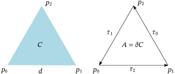
Figure 4.1. The triangle and its boundary as polyhedral chains for Example 4.2.

Then,

$$\|A\|^{\flat}=\|\partial C\|^{\flat}\leqslant\left|C\right|=\frac{\sqrt{3}}{4}d^{2}.$$ (4.11)

It is noted that $\|A\|^{\flat}$ is bounded by $d^{2}$ while $\left|A\right|$ behaves like $d$.

Example 4.3.

The von Koch snowflake is a standard example of a fractal constructed, for example, as follows. One starts with the $1$-simplex $B_{0}$ of unit length and at each step one sets,

$$B_{i}=B_{0}+\sum_{j=1}^{i}A_{j},$$ (4.12)

as illustrated in Figure 4.2.

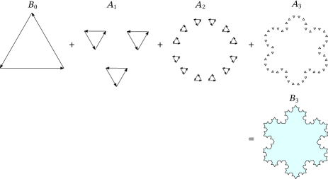
Figure 4.2. An illustration of the construction of the snowflake as a flat chain for Example 4.3.

Now,

$$A_{j}=\sum_{l=1}^{3\cdot 4^{j-1}}A_{jl},$$ (4.13)

where $A_{jl}$ is the oriented boundary of a triangle of sides $3^{-i}$. The triangles are situated in such a way, that at each step, the middle third of the edge of the previous step is canceled.

The length of the resulting curve is unbounded and has the Hausdorff dimension $\ln 4/\ln 3$. Since at each triangle adds two segments of size $3^{-j}$, the total length added at the $j$-th step is

$$3\cdot 4^{j-1}\cdot 2\cdot 3^{-j}=\frac{3}{2}\left(\frac{4}{3}\right)^{j}.$$ (4.14)

On the other hand, the flat norm of each $A_{jl}$ is bounded by the area of the corresponding triangle,

$$\|A_{jl}\|^{\flat}\leqslant\frac{1}{2}\Bigl{(}\frac{\sqrt{3}}{2}3^{-j}\Bigr{)}3^{-j}=\frac{\sqrt{3}}{4}3^{-2j}.$$ (4.15)

Thus,

$$\begin{split}\|A_{j}\|^{\flat}&=\biggl{\|}\sum_{l=1}^{3\cdot 4^{j-1}}A_{jl}\biggr{\|}^{\flat},\\ &\leqslant\sum_{l=1}^{3\cdot 4^{j-1}}\|A_{jl}\|^{\flat}\\ &\leqslant 3\cdot 4^{j-1}\frac{\sqrt{3}}{4}3^{-2j},\\ &=\frac{3\sqrt{3}}{16}\left(\frac{4}{9}\right)^{j}.\end{split}$$ (4.16)

It follows that for $k>i$,

$$\begin{split}\|B_{k}-B_{i}\|^{\flat}&=\biggl{\|}\sum_{j=i+1}^{k}A_{j}\biggr{\|}^{\flat},\\ &\leqslant\sum_{j=i+1}^{k}\|A_{j}\|^{\flat},\\ &\leqslant\sum_{j=i+1}^{k}\frac{3\sqrt{3}}{16}\left(\frac{4}{9}\right)^{j}\\ &\leqslant\sum_{j=i+1}^{\infty}\frac{3\sqrt{3}}{16}\left(\frac{4}{9}\right)^{j},\end{split}$$ (4.17)

which is a convergent geometric series, the first term of which tends to zero as $i\to\infty$. We conclude that this is a Cauchy sequence and its limit, the snowflake, is a flat chain. Let us remark that the resulting curve does not induce a flat cochain but a current of different type. For example, integration on the resulting curve is possible using the corresponding Hausdorff measure.

Remark 4.4.

When constructed as above using equilateral triangles, the Hausdorff dimension of the von Koch curve is $\ln 4/\ln 3>1$. Variants of the standard von Koch snowflake are obtained when the typical triangles added are general isosceles triangles (see an illustration in Figure 4.3). In such a case, the Hausdorff dimension of the curve can be any number between $1$ and $2$.

Figure 4.3.
(a) A typical equilateral triangle in the construction of the snowflake.
(b) A different snowflake. The type of snowflake depends on the vertex angle. Here (a) is a standard snowflake.

To relate Whitney’s theory of flat chains to de Rham currents we note that Federer [Fed69], defines flat chains as a particular subspace of de Rham currents in open subsets of $\mathbb{R}^{n}$. His construction may be roughly described as follows. Given an open subset $U\subset\mathbb{R}^{n}$, let $K\subset U$ be a compact subset. The flat seminorm relative to $K$ of an $r$-form $\varphi$ on $U$ is defined as

$$\|\varphi\|_{K}^{\flat}:=\sup_{x\in K}\{\left|\varphi(x)\right|,\left|\textrm{d}\varphi(x)\right|\},$$ (4.18)

where one uses the natural metric structure of $\mathbb{R}^{n}$ to evaluate $\left|\varphi(x)\right|$ and $\left|\textrm{d}\varphi(x)\right|$. Then, a current supported in $K$ is a flat chain if it is continuous relative to the norm $\|\cdot\|_{K}^{\flat}$.

5. Fractal Growth

In this section, we demonstrate growth processes that are associated with fractal bodies. For example, let

$$\mathcal{R}=[0,1]\times\{0\}\subset\mathbb{R}^{2},$$ (5.1)

and let $Q\subset[0,1]$ be and arbitrary Cantor set. Then, the evolving set

$$\mathcal{R}_{t}=[0,1]\cup(Q\times[0,t])$$ (5.2)

represents a growing fractal that may be applicable in the description of percolation processes.

Next, we demonstrate a continuous growth process of a polyhedral chain into a fractal. Specifically, we consider a continuous version of the construction of the von Koch snowflake in Example 4.3. The notation and terminology of Example 4.3 will be used below with the following modifications.

The triangles $A_{ij}$ are now time-dependent isosceles triangles. The bases of the triangles are $d_{i}=3^{-i}$ and they are situated in the middle thirds as before, but the heights of the triangles $h_{i}(t)$ are time-dependent (see Figure 5.1).

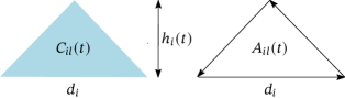
Figure 5.1. The triangles for the construction of the continuous construction of the snowflake.

For the time-interval $t\in[0,1]$ and $i=1,\dots,\infty$, we consider the intervals $\Delta_{i}=(t_{i-1},t_{i}]$ of lengths $\Delta t_{i}=2^{-i}$ and the instances $t_{i}=t_{i-1}+\Delta t_{i}$, where $t_{0}=0$. Thus,

$$t_{i}=\sum_{j=1}^{i}\Delta t_{i}=1-2^{-i}.$$ (5.3)

If $t\in\Delta_{i}$, we set $\tau=t-t_{i-1}$.

We define the function $h:(0,1)\longrightarrow[0,1]$ such that

$$h(t)=2^{i}\tau.$$ (5.4)

It follows that $h(t_{i})=2^{i}\Delta_{i}=1$.

Figure 5.2. The function $h(t)$

Thus, we define the height of the triangle $h_{i}(t)$ as

$$h_{i}(t):=\frac{\sqrt{3}}{2}d_{i}h(t)=\frac{\sqrt{3}}{2}\left(\frac{2}{3}\right)^{i}\tau,\qquad t\in\Delta_{i}$$ (5.5)

so that

$$h_{i}(t)\overset{t\to t_{i-1}}{\longrightarrow}0,\qquad\text{and}\qquad h_{i}(t_{i})=\frac{\sqrt{3}}{2}d_{i}.$$ (5.6)

We can formally extend $h_{i}$ by setting

$$h_{i}(t):=\begin{cases}0,&\text{for }t\leqslant t_{i-1},\\ 1,&\text{for }t>t_{i}.\end{cases}$$ (5.7)

It is noted that the dependence of $i$ on $t$ can be obtained as follows. If $t\in\Delta_{i}$, then

$$i-1<-\log_{2}(1-t)\leqslant i.$$ (5.8)

Using the floor, $\left\lfloor\cdot\right\rfloor$, and ceiling $\lceil\cdot\rceil$ functions, it is concluded that

$$i=\lceil-\log_{2}(1-t)\rceil,\qquad i-1=\lfloor-\log_{2}(1-t)\rfloor.$$ (5.9)

Defining the function

$$I(t):=\lceil-\log_{2}(1-t)\rceil,$$ (5.10)

Equation (5.9) may be written as $i=I(t).$

Hence,

$$\begin{split}\tau&=t-t_{i-1},\\ &=t-(1-2^{-(i-1)}),\\ &=t-1+2^{-\lfloor-\log_{2}(1-t)\rfloor},\end{split}$$ (5.11)

and using $-\lfloor-x\rfloor=\lceil x\rceil$,

$$\tau=t+2^{\lceil\log_{2}(1-t)\rceil}-1.$$ (5.12)

At each interval $\Delta_{i}$ the chains

$$A_{i}(t)=\sum_{l=1}^{3\cdot 4^{i-1}}A_{il}(t),$$ (5.13)

with $A_{il}(t)$ as defined above in terms of $h_{i}(t)$, are added continuously starting from zero height to equilateral triangles. Thus, equation (4.12) is replaced by

$$B(t)=B_{0}+\sum_{i=I(T)=1}^{\infty}A_{i}(t)=B_{0}+\sum_{j=1}^{I(t)-1}A_{j}+A_{I(t)}(t),$$ (5.14)

where it is noted that by definition, only one term in the infinite sum is different than zero, and we use the notation $A_{i}:=A_{i}(t_{i})$.

As $t\to 1$, the flat chain converges to the snowflake.

Finally, we note that integration theory of forms over chains on manifolds and the corresponding Stokes theorem, implies that the setting of (3.11) for surface growth applies here also for any time $t_{0}<1$. We consider the chain $\mathcal{R}$ defined as follows. Let $C(t)$ be the chain bounded by $B(t)$, so that $B(t)=\partial C(t),$ and set

$$\mathcal{R}=\bigcup_{t_{0}>t^{\prime}>t}\{(t^{\prime},x)\mid x\in C(t),\;0\leqslant t\leqslant t_{0}\}.$$ (5.15)

(Note that we have an artificial component of the boundary at $t_{0}$, where all points are lost.)

This example demonstrates a continuous process of growth in which the perimeter of the body grows without bound while the area of the body remains bounded. Such a process may be advantageous when the objective is increasing the transport through the boundary.

This heuristic description of “added continuously starting from zero height to equilateral triangles” has a more precise formal interpretation. For any $t$ and any $h_{i}(t)$, the new body $A_{i}(t)$ has a Lipschitz (even piecewise linear) boundary, i.e., any of these bodies is a Lipschitz domain. The procedure above is a mathematical description of an evolution of Lipschitz domains into the snowflake (Figure 4.2).

Evolution of Smooth Bodies to Fractals

In this section we present a construction that enables a mathematical description of the evolution of two-dimensional bodies having smooth boundaries into bodies with fractal boundaries (see an illustration in Figure 5.3).

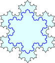
Figure 5.3. Illustrating the evolution of a smooth boundary into a fractal one. (The black line represents the boundary of the snowflake, and the blue line represents the smooth boundary of an approximation in the growth process.)

Let $B(0,t)\subset\mathbb{R}^{2}$ denote the open disk centered at the origin of radius $t$, and let $G$ be an arbitrary simply connected bounded open domain in $\mathbb{R}^{2}$ representing a body, the boundary of which may be fractal. By the Riemann mapping theorem, there is a conformal diffeomorphism

$$\phi:B(0,2)\longrightarrow G.$$ (5.16)

Consider the set

$$\mathcal{R}_{1}:=\phi\{\overline{B(0,1)}\},$$ (5.17)

where the overline indicates closure. It follows that $\partial\mathcal{R}_{1}$ is smooth.

The domain $\mathcal{R}_{1}$ represents the initial state of the growing body, at time $t=1$ and we want to describe its evolution to a body $\mathcal{R}_{2}$ having a fractal boundary at time $t=2$. Thus, for $t\in[1,2)$, we set

$$\mathcal{R}_{t}:=\phi\{\overline{B(0,t)}\}.$$ (5.18)

Let

$$s_{t}:\mathbb{R}^{2}\longrightarrow\mathbb{R}^{2},\qquad s_{t}(x)=tx$$ (5.19)

and consider the conformal diffeomorphism

$$\phi_{t}:\mathcal{R}_{1}\longrightarrow\mathcal{R}_{t},\qquad\phi_{t}(x)=\phi\circ s_{t}\circ\phi^{-1}(x).$$

By the theory of prime ends (see, for example, [Eps81], [BCDM20, Chap. 4]), the mapping $\phi$ can be extended to the “ideal” Carath odory boundary of $G$. If the topological boundary of $G$ is locally connected at any boundary point, the Carath odory boundary coincides with the topological boundary.

Regions in the plane with fractal boundaries, similar to the von Koch snowflake above, satisfy this condition. In such a case, the fractal boundary may be denoted as $\partial\mathcal{R}_{2}$. Thus, during the time interval $[1,2]$, the smooth boundary $\partial\mathcal{R}_{1}$ evolved into the fractal $\partial\mathcal{R}_{2}$.

References

- [Bar88] M.F. Barnsley. Fractals Everywhere. Academic Press, 1988.
- [BCDM20] F. Bracci, M.D. Contreras, and S. Díaz-Madrigal. Continuous Semigroups of Holomorphic Self-maps of the Unit Disc. Springer, 2020.
- [dR84] G. de Rham. Differentiable Manifolds. Springer, 1984.
- [Eps81] D.B.A. Epstein. Prime ends. Proceedings of the London Mathematical Society, 42:385–414, 1981.
- [Fed69] H. Federer. Geometric Measure Theory. Springer, 1969.
- [FM89] H. Fujikawa and M. Matsushita. Fractal growth of Basillus sublitis on agar plates. Journal of the Physical Society of Japan, 58:3875–3878, 1989.
- [FM91] H. Fujikawa and M. Matsushita. Bacterial fractal growth in the concentration field of nutrient. Journal of the Physical Society of Japan, 60:88–94, 1991.
- [GKS82] V. Goldshtein, V. Kuzminov, and I. Shvedov. Differential forms on a Lipschitz manifold. Sibirskii Matematicheskii Zhurnal, 32(2):16–30, 1982. English transl.: Siberian Math. J., 23, 151–161.
- [GP23] V. Goldshtein and R. Panenko. A Lipschitz version of de Rham theorem for -cohomology. Transactions of A. Razmadze Mathematical Institute, 177(2):189–204, 2023.
- [GS23] V. Goldshtein and R. Segev. Notes on smooth and singular volumetric growth, 2023. arXiv:2311.06902v1 [math-ph].
- [OPS90] M. Obert, P. Pfeifer, and M. Sernetz. Microbial growth patterns described by fractal geometry. Journal of Bacteriology, 172:1180–1185, 1990.
- [PY23] S.P. Pradhan and A. Yavari. Accretion-ablation mechanics. arXiv:2307.00159v3, 2023. arXiv:2307.00159v3.
- [RS03] G. Rodnay and R. Segev. Cauchy’s flux theorem in light of geometric integration theory. Journal of Elasticity, 71:183–203, 2003.
- [SC89] R.B. Stinchcombe and E. Courtens. Fractal, phase transitions and criticality [and discussion]. Proceedings of the Royal Society of London A, 423:17–33, 1989.
- [SDM+82] R. Skalak, G. Dasgupta, M. Moss, E. Otten, P. Dullemeijer, and H. Vilmann. Analytical description of growth. Journal of Theoretical Biology, 94:555–577, 1982.
- [SE96] R. Segev and M. Epstein. On theories of growing bodies. In R.C. Batra and M.F.Beatty, editors, Contemporary Research in the Mechaincs and mathematics of Materials, dedicated to J.L. Ericksen 70th birthday, pages 119–130. CIMNE, Barcelona, 1996.
- [SE22] R. Segev and M. Epstein. Proto-Galilean dynamics of a particle and a continuous body. Journal of Elasticity, 2022. Special issue in memory of J. Ericksen, https://doi.org/10.1007/s10659-022-09929-w.
- [Seg23] R. Segev. Foundations of Geometric Continuum Mechanics. Birkhauser, 2023.
- [Suz83] M. Suzuki. Phase transition and fractals. Progress of Theoretical Physics, 69:65–76, 1983.
- [SY16] Fabio Sozio and Arash Yavari. Nonlinear mechanics of surface growth for cylindrical and spherical elastic bodies. Journal of the Mechanics and Physics of Solids, 98, 08 2016.
- [Tab95] R.A. Taber. Biomechanics of growth, remodeling, and morphogenesis. Applied Mechanics Reviews, 48:486–545, 1995.
- [TZ19] L. Truskinovsky and G. Zurlo. Nonlinear elasticity of incompatible surface growth. Physical Review E, 99:053001, 2019.
- [WBFW22] X. Wang, R. Blumenfeld, X.-Q. Feng, and D. A. Weitz. Phase transitions in bacteria - From structural transitions in free living bacteria to phenotypic transitions in bacteria within biofilms. Physics of Life Reviews, 43:98, 2022. DOI: 10.1016/j.plrev.2022.09.004.
- [Whi57] H. Whitney. Geometric Integration Theory. Princeton University Press, 1957.