Dirac zeros in an orbital selective Mott phase:Green’s function Berry curvature and flux quantization

Abstract

How electronic topology develops in strongly correlated systems represents a fundamental challenge in the field of quantum materials. Recent studies have advanced the characterization and diagnosis of topology in Mott insulators whose underlying electronic structure is topologically nontrivial, through “Green’s function zeros”. However, their counterparts in metallic systems have yet to be explored. Here, we address this problem in an orbital-selective Mott phase (OSMP), which is of extensive interest to a variety of strongly correlated systems with a short-range Coulomb repulsion. We demonstrate symmetry protected crossing of the zeros in an OSMP. Utilizing the concept of Green’s function Berry curvature, we show that the zero crossing has a quantized Berry flux. The resulting notion of Dirac zeros provides a window into the largely hidden landscape of topological zeros in strongly correlated metallic systems and, moreover, opens up a means to diagnose strongly correlated topology in new materials classes.

Introduction.   Quantum fluctuations as promoted by strong correlations drive novel electronic phases of matter  Keimer and Moore (2017); Paschen and Si (2021), and this also applies when the underlying electronic structure is topologically nontrivial Stormer et al. (1999); Xie et al. (2021); Zeng et al. (2023); Lu et al. (2023); Lai et al. (2018); Dzsaber et al. (2017, 2021); Chen et al. (2022). One important question is how to diagnose electronic topology in the strongly correlated settings. In band theory of noninteracting crystalline systems, lattice symmetries constrain the one-electron eigenstates–the Bloch states–and serve as indicators for topology Armitage et al. (2018); Nagaosa et al. (2020); Bradlyn et al. (2017); Cano et al. (2018); Po et al. (2017); Watanabe et al. (2016); they uniquely determine the representations Cano et al. (2018) of the Bloch states and justify the robustness of band degeneracies in the energy dispersion Cano and Bradlyn (2021). In interacting systems, a fundamental quantity is the single-particle Green’s function Abrikosov et al. (2012), which describes the frequency and wavevector-resolved propagation of an electron in the many-particle environment. The eigenvectors of the Green’s function form a representation of the space group Hu et al. (2021). In addition, these eigenvectors allow for the introduction of a Green’s function Berry curvature Setty et al. (2023a).

Mott insulators develop when the Coulomb repulsion is strong (and the band filling is commensurate). They have been known to feature Green’s function zeros Dzyaloshinskii (2003); Essin and Gurarie (2011); You et al. (2018), contours in frequency-momentum space at which the Green’s function vanishes. The roles of these zeros in the topology of Mott insulators have recently gained considerable interest Setty et al. (2023b); Wagner et al. (2023a) in the presence of topological noninteracting bands Morimoto and Nagaosa (2016). In particular, it was shown that symmetry constraints based on Green’s function eigenvectors also act on the zeros Setty et al. (2023b). Moreover, the notion of Green’s function Berry flux quantization has been illustrated in a Mott insulator derived from long-ranged interactions Setty et al. (2023a). The quantized flux of the zeros serves as a means to search for topological Mott insulators.

In this work, we address whether and how Green’s function zeros can play a role in the topology of correlated metallic systems. To this end, we study an orbital-selective Mott phase, arising in correlated multi-orbital systems when a subset of the orbitals are (on the verge of being) localized. OSMP and its proximate regimes are increasingly being recognized as important to a variety of strongly correlated materials platforms Paschen and Si (2021); Kirchner et al. (2020); Si et al. (2001); Coleman et al. (2001); Senthil et al. (2004); Anisimov et al. (2002); Yi et al. (2017); Si and Hussey (2023); Zhao et al. (2023a); Guerci et al. (2023); Xie et al. (2023); Zhao et al. (2023b); Hu and Si (2023); Huang et al. . Furthermore, we consider a local Coulomb repulsion. We show that symmetry protected zero crossings occur and demonstrate the notion of Dirac zeros in terms of a quantization of the Green’s function Berry flux. Given that the orbital-selective Mott physics is prevalent across the strongly correlated metallic systems, our work opens up an important new avenue to realize strongly correlated topological matter.

Model and Methods.   We consider a four-orbital interacting Hamiltonian defined on a cubic lattice, taking the form of $\mathcal{H}=\mathcal{H}_{0}+\mathcal{H}_{int}$.

The noninteracting part preserves a U(1)-spin rotational symmetry along the $z$-axis; in accordance, $\mathcal{H}^{\uparrow}_{0}=[\mathcal{H}^{\downarrow}_{0}]^{\dagger}$. The kinetic Hamiltonian for the spin-$\uparrow$ electrons is given by $\mathcal{H}_{0}^{\uparrow}=\sum_{\bm{k}}\Psi_{\bm{k}\uparrow}^{\dagger}H_{0}^{\uparrow}(\bm{k})\Psi_{\bm{k}\uparrow}$, where $\Psi_{\bm{k}\uparrow}=[\psi_{Ah\uparrow},\psi_{Bh\uparrow}\psi_{Al\uparrow},\psi_{Bl\uparrow}]^{T}$, with subscripts $\tau=A/B$ and $o=h/l$ introduced to distinguish the sublattices and heavy/light orbitals, respectively.

$$H_{0}^{\uparrow}(\bm{k})=\begin{pmatrix}H_{0,hh}^{\uparrow}(\bm{k})&H_{0,hl}^{\uparrow}(\bm{k})\\ [H_{0,hl}^{\uparrow}(\bm{k})]^{\dagger}&H_{0,ll}^{\uparrow}(\bm{k})\end{pmatrix},$$ (1)

in which $H_{0,hh/ll}^{\uparrow}(\bm{k})=2t_{h}/t_{l}(\cos k_{x}+\cos k_{y}+\cos k_{z})\tau_{z}+2t_{h/l}^{soc}(\sin k_{x}\tau_{x}+\sin k_{y}\tau_{y})$ and $H_{0,hl}^{\uparrow}(\bm{k})=2t_{hl}(\cos k_{x}+\cos k_{y}+\cos k_{z})$. $\tau_{x/y/z}$ are the Pauli matrices acting on the sublattice space. Furthermore, $t_{h}$ ($t_{l}$) and $t_{h}^{soc}$ ($t_{l}^{soc}$) denote the nearest neighbor direct hopping and spin-orbit coupling between the heavy (light) orbitals, respectively, while $t_{hl}$ represents the nearest neighbor hopping between the heavy and light orbitals. We consider $|t_{h}|$ to be considerably smaller than $|t_{l}|$, such that for the same interaction strength, the heavy orbitals are much more correlated than the light orbitals. Without a loss of generality, we adopt the following parameters: $t_{h}=1$, $t_{h}^{soc}=0.6$, $t_{l}=4$, $t_{l}^{soc}=2.4$ and $t_{hl}=1.5$.

We will consider the effect of an onsite Coulomb repulsion. Our focus will be on a range of interactions that are small compared to the light bandwidth and, accordingly, have a relatively weak effect on the light band. Thus, for simplicity, we will study only the effect of an intraorbital Hubbard interaction that acts on the heavy orbitals:

$$\mathcal{H}_{int}=\sum_{\tau}\frac{U}{2}\left(n_{\tau h\uparrow}+n_{\tau h\downarrow}-1\right)^{2}\,,$$ (2)

where the index $\tau$ enumerates the two subalttices of the heavy orbitals. The model contains a $C_{4z}$ rotational symmetry, which protects the gapless Dirac points in the weak coupling region.

Dispersive zeros may arise only if the electron self-energy is ${\bf k}$-dependent. To capture such effects, we develop a cluster version of the U(1)-slave-spin (SS) method Yu and Si (2012). In the U(1)-SS approach, an electronic operator is expressed as $\psi_{i\tau o\sigma}^{\dagger}=S^{+}_{i\tau o\sigma}f_{i\tau o\sigma}^{\dagger}$, where the SS operator $S^{+}$ is introduced to carry the charge degree of freedom and the auxiliary fermion $f^{\dagger}$ the spin degree of freedom in the form of a “spinon” operator. The enlarged Hilbert space spanned by the SS and auxiliary fermion is limited to the physical ones when we impose the constraint $S_{i\tau o\sigma}^{z}+1/2=f^{\dagger}_{i\tau o\sigma}f_{i\tau o\sigma}$. We treat the Hamiltonian in the SS representation at the saddle-point level, which leads to two decoupled effective Hamiltonians, each containing only the SS or auxiliary fermions, respectively [See the supplementary materials (SM)]. Furthermore, we exactly diagonalize the SS Hamiltonian which is constrained on a finite cluster that is embedded in an effective medium; here, we consider a cluster size of two unit cells.

The Mott transition of an orbital is signaled by the vanishing of its quasiparticle weight, which is determined from $Z_{i\tau o\sigma}=|\langle S_{i\tau o\sigma}^{+}\rangle|^{2}$. The spatial fluctuations are captured by the bond operators $\chi^{f}_{i\tau o\sigma,j\tau^{\prime}o^{\prime}\sigma^{\prime}}=\langle S^{+}_{i\tau o\sigma}S^{-}_{j\tau^{\prime}o^{\prime}\sigma^{\prime}}\rangle$. Further details of the method and its context are given in the SM.

Orbital selective Mott phase.   In the noninteracting limit, the Hamiltonian describes two species of semimetals, each associated with one kind of orbital and each having four gapless (Dirac) points sitting at the momenta $(\pi,0,\pm\frac{\pi}{2})$ and $(0,\pi,\pm\frac{\pi}{2})$. The system contains both the time-reversal ($\mathcal{T}$) and inversion ($\mathcal{I}$) symmetries. The discrete rotation $C_{4z}$ symmetry protects the Dirac crossings along the high symmetry lines paralleled to the $z$-axis. The noninteracting band structure along the high symmetry line $X-R$ is displayed in Fig. 1(b), showing a symmetry protected Dirac node.

We are now in position to discuss the correlation effect. As depicted in Fig. 1(c), the quasiparticle weight of the heavy orbitals monotonically decreases as we increase the strength of the intra-orbital on-site Hubbard interaction. It eventually diminishes to zero at a critical value $U_{c}/t_{h}=9.5$. Notice that, the effective interorbital hybridization between the heavy and light electrons equals to $\sqrt{Z_{h}}t_{hl}$, which also vanishes in the OSMP. In other words, the heavy electrons are decoupled from the light ones in the OSMP, leading to the notion of correlation-driven dehybridization, which is analogous to the Kondo-destroyed fixed point of heavy fermion systems Si et al. (2001); Coleman et al. (2001); Senthil et al. (2004). Such a dehybridization fixed point is realized from the competition between the hybridization and spatial correlations, which protects the stability of the OSMP Yu and Si (2017); Komijani and Kotliar (2017).

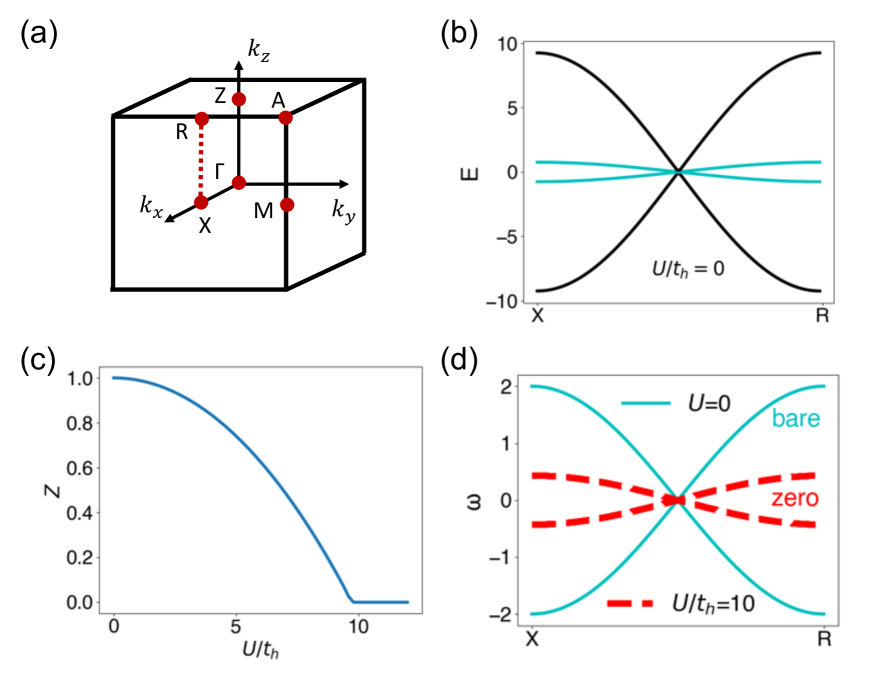
Figure 1: (a) Brillouin zone of a cubic lattice, with high symmetry points marked. (b) The non-interacting band structure of the narrow (cyan) and wide (black) bands along a high symmetry line ($X-R$), showing a Dirac node protected by symmetry. (c) Quasiparticle weight of the heavy electrons as a function of the onsite interaction $U$. (d) Red dashed lines: Green’s function zeros in the OSMP phase, for $U/t_{h}=10$, dispersing along $X-R$. Cyan solid lines: Dispersion of the bare narrower-band electrons, at $U=0$.

Dirac nodes of Green’s function zeros.  We now turn to the single particle Green’s function. In the SS approach, it is represented by the SS and auxiliary fermions as $G_{\sigma}^{\tau o\tau^{\prime}o^{\prime}}(i-j,\tau)=-\langle T_{\tau}S_{i\tau o\sigma}^{-}(\tau)S_{j\tau^{\prime}o^{\prime}\sigma}^{+}(0)f_{i\tau o\sigma}(\tau)f_{j\tau^{\prime}o^{\prime}\sigma}^{\dagger}(0)\rangle$. At the saddle-point level, the Green’s function is decomposed into coherent and incoherent parts as follows:

$$G^{\tau o\tau^{\prime}o^{\prime}}(\bm{k},i\omega_{n}) =\sqrt{Z_{\tau o}Z_{\tau^{\prime}o^{\prime}}}G^{\tau o\tau^{\prime}o^{\prime}}_{f}(\bm{k},i\omega_{n})$$ (3)

$$+G_{incoh}^{\tau o\tau^{\prime}o^{\prime}}(\bm{k},i\omega_{n})\,.$$

In the coherent part, $G_{f}^{\tau o\tau^{\prime}o^{\prime}}$ represents the Green’s function of the auxiliary fermion. In our case, the quasiparticle weights ($Z_{\tau l}$) for the light orbitals are equal to $1$ across the whole phase diagram. In the OSMP phase, the heavy electrons completely lose their coherence and, thus, the coherent part of the Green’s function is entirely comprised of the light orbitals. On the other hand, the incoherent part of the Green’s function is uniquely contributed by the heavy orbitals. The momentum-resolved incoherent Green’s function is obtained by a Fourier transform of the real space counterpart. This leads to

$$G_{incoh}^{\tau o\tau^{\prime}o^{\prime}}(\bm{k},i\omega_{n}) =G^{\tau o\tau^{\prime}o^{\prime}}_{incoh}(\bm{0},i\omega_{n})$$ (4)

$$+\sum_{\bm{R}\neq\bm{0}}e^{i\bm{k}\cdot\bm{R}}G_{incoh}^{\tau o\tau^{\prime}o^{\prime}}(\bm{R},i\omega_{n})\,,$$

where $\bm{R}$ enumerates through the separations between the unit cells. The specific expressions of $G^{\tau o\tau^{\prime}o^{\prime}}_{incoh}(\bm{0},i\omega_{n})$ and $G_{incoh}^{\tau o\tau^{\prime}o^{\prime}}(\bm{R},i\omega_{n})$ are shown in the SM.

We focus on the OSMP, which is illustrated with the choice of the interaction strength $U/t_{h}=10$. We calculate the determinant of the retarded Green’s function $|\det G(\bm{k},\omega+i0^{+})|$ for the heavy orbitals in order to look for the zeros of the interacting single-particle Green’s function.

To further elaborate on the electronic properties in the OSMP, we show the spectrum function for the heavy orbitals in Fig. 2(a), which is calculated from $\rho^{h}(\bm{k},\omega)=-\frac{1}{\pi}\sum_{\tau\sigma}G^{\tau h\tau h}_{\sigma}(\bm{k},\omega+i0^{+})$. The lower and upper Hubbard bands are separated by a Mott gap as marked by the arrow shown in Fig. 2(a). We then turn to discussing the frequency resolved determinant of the Green’s function. Its frequency dependence at $\bm{k}=(\pi,0,0)$ and $\bm{k}=(\pi,0,\frac{\pi}{2})$ is respectively displayed in Figs. 2(b,c) on a logarithmic scale. The lower and upper Hubbard bands correspond to the broad shoulder-like peaks at high frequencies. Whereas the Green’s function zeros, marked by the black arrows, reside within the Mott gap. Different from the case of momentum $X$, which is shown in Fig. 2(b), only one dip is observed at momentum $\bm{k}=(\pi,0,\pi/2)$ [Fig. 2(c)], showing that the Green’s function zeros are merged at this momentum.

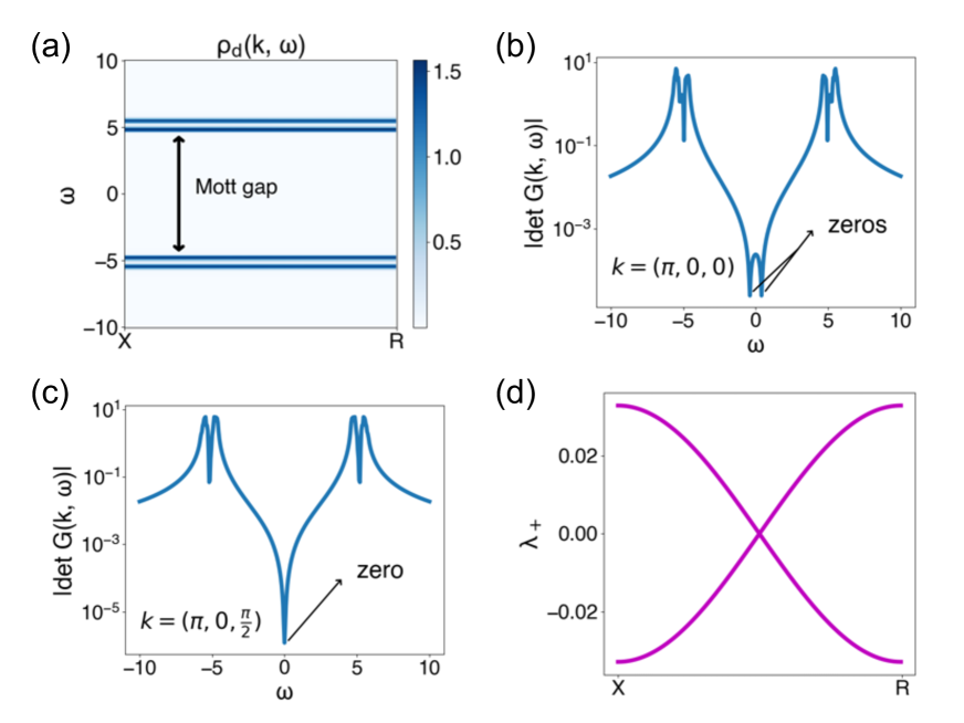
Figure 2: (a) The energy distribution of the total spectral function along $X-R$, at $U/t_{h}=10$. The Mott gap is marked. (b) and (c), The variance of $|\det G(\bm{k},\omega)|$ for the heavy orbitals versus $\omega$, demonstrating the Green’s function zeros, at $\bm{k}=(\pi,0,0)$ and $\bm{k}=(\pi,0,\pi/2)$, respectively, (d) Eigenvalues of $G_{+}(\bm{k},\omega)$ at fixed frequency $\omega=0$, along the high symmetry line $X-R$.

The collection of zeros at the different wavevectors is depicted in Fig. 1(d). The red dashed lines show the dispersive zeros along the high symmetry line $X-R$. Furthermore, two branches of Green’s function zeros merge exactly at momentum for the Dirac node of the bare heavy electrons in the noninteracting limit, which are denoted by the cyan solid lines in Fig. 1(d). (Here, “bare” means both at $U=0$ and without a hybridization between the heavy and light electrons.) This result demonstrates the presence and robustness of the “gapless” node coming from the Green’s function zeros in the strongly correlated limit, and motivates us to use the eigenvectors of the Green’s function zeros (instead of Green’s function poles) to diagnose the topology in such strongly correlated systems.

Quantization of Green’s function Berry flux.   In the noninteracting limit, the winding of the Bloch functions in the momentum space is used to calculate the Berry flux quantization. The question is how to define an appropriate Berry phase for the strongly correlated case. Here, we use a frequency-dependent Berry curvature from the Green’s function eigenvectors, which has recently been introduced Setty et al. (2023a).

We define a Hermitian combination:

$$G_{+}(\bm{k},\omega)=G^{R}(\bm{k},\omega)+G^{A}(\bm{k},\omega)\,,$$ (5)

where $G^{R,A}$ are the retarded and advanced Green’s functions. We focus on this combination (as opposed to, say, $G_{+}^{-1}$) because it is regular across the zeros in the frequency-momentum space. The $\alpha$-th eigenvalues and eigenvectors of the new Green’s function are obtained by the eigenvalue equation,

$$G_{+}(\bm{k},\omega)|\phi_{\alpha}(\bm{k},\omega)\rangle=\lambda_{+}^{\alpha}|\phi_{\alpha}(\bm{k},\omega)\rangle\,.$$ (6)

Because of the Hermiticity, the eigenvalues $\lambda_{+}$ are always real. The eigenvalues of $G_{+}$ at $\omega=0$ is depicted in Fig. 2(d). Similar to the noninteracting bands and Green’s function zeros, along the same high symmetry line, the “band”s show a nodal crossing at the middle point of $X-R$.

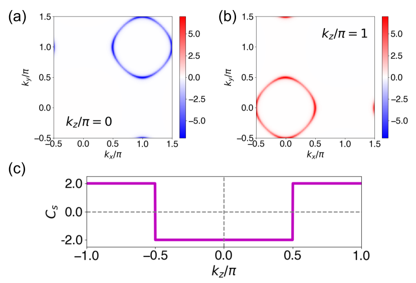
Figure 3: (a) and (b), The Green’s function Berry curvature, $B_{z}^{\uparrow}(\bm{k},\omega)$, for frequency $\omega=0$, in the $k_{z}=0$ and $k_{z}=\pi$ planes, respectively. (c) The spin Chern number obtained from the Green’s function Berry curvature as a variance of $k_{z}$ at the fixed frequency $\omega=0$, demonstrating the quantization of the corresponding Berry flux around the Dirac node of zeros.

Furthermore, from the “energy” (eigenvalues $\lambda_{+}$) of the “bands”, we are able to define the Berry curvature associated with the eigenvectors at momentum $\bm{k}$ and freqeuncy $\omega$. It takes the form of

$$B_{m}(\bm{k},\omega)=\sum_{\alpha,ij}\epsilon_{ijm}\left[\langle\partial_{i}\phi_{\alpha}(\bm{k},\omega)|\partial_{j}\phi_{\alpha}(\bm{k},\omega)\rangle\right]\,,$$ (7)

where $\alpha$ sums over the “bands” with eigenvalue $\lambda_{+}^{\alpha}$ smaller than $0$, and $\epsilon_{ijm}$ is the Levi-Civita symbol. For a given $k_{z}$ and $\omega$, a frequency dependent spin Chern number is then calculated by

$$C_{s}(\omega,k_{z})=\frac{i}{2\pi}\sum_{\sigma}(-1)^{\sigma}\int d\bm{k}_{\perp}B_{z}^{\sigma}(\bm{k}_{\perp},k_{z},\omega)\,.$$ (8)

with $\bm{k}_{\perp}=(k_{x},k_{y})$, and $\sigma=0(1)$ for spin-$\uparrow$($\downarrow$).

We focus on the case $\omega=0$. The Berry curvatures (spin-$\uparrow$) at $k_{z}=0$ and $k_{z}=\pi$ planes are displayed in Figs. 3(a,b), which are seen to have different signs. Their distribution in the $k_{x}-k_{y}$ plane captures the dispersion of the Green’s function “bands”. We find them to be quantized in both planes after integrating the Berry curvature over the whole Brillouin zone plane. We further scan the Chern numbers $C_{s}$ as a function of $k_{z}$, which are shown in Fig. 3(c). There is a sudden jump by a value of $4$, when the cutting plane crosses the nodal points at $k_{z}=\pm\pi/2$. There are two nodes at each of the $k_{z}=\pi/2$ and $k_{z}=-\pi/2$ planes (as can be inferred from the SM, Fig. 4). Accordingly, there is a jump of $2$ across each crossing.

The quantization of the Berry flux shows an enclosed monopole charge at a touching point of the Green’s function bands. Given that the zero crossing has a four-fold degeneracy and a quantized Green’s function monopole charge, we will refer to it as a Dirac zero.

Discussion.   Several remarks are in order. Firstly, by using the Green’s function Berry flux, we have defined the notion of Dirac zeros. We expect that this can be readily extended to other settings, such as Weyl zeros in correlated systems with broken inversion or time-reversal symmetry. Secondly, our work provides a systematic approach to diagnose the electronic topology in the correlation-driven orbital selective Mott phase. In addition to heavy fermion metals, orbital-selective Mott correlations have been extensively discussed in Fe-based superconductors Yi et al. (2017); Si and Hussey (2023) and are also being recognized in both the moiré structures Zhao et al. (2023a); Guerci et al. (2023); Xie et al. (2023); Zhao et al. (2023b) and geometry-induced flat band compounds Hu and Si (2023); Huang et al. . Many of these systems contain topological electron bands. As such, the notion of Dirac/Weyl zeros serves as a diagnostic tool to search and obtain new types of strongly correlated topological phases and materials. Finally, it has been increasingly recognized that the Green’s function zeros contribute to measurable physical quantities, such as the Luttinger volume Seki and Yunoki (2017); Setty et al. (2023c), Hall effect Setty et al. (2023c); Blason and Fabrizio (2023); Peralta Gavensky et al. (2023); Zhao et al. (2023c) and even quantum oscillations Fabrizio (2022); Setty et al. (2023a) in a consistent way Setty et al. (2023c). Consequently, the topological feature defined from Green’s function zeros is expected to influence physical properties in a nontrivial manner. This exciting prospect warrants further exploration.

Conclusion.   In a multiorbital model with topological bandstructure, we have demonstrated a symmetry protected crossing of Green’s function zeros in its orbital-selective Mott phase (OSMP). Through the concept of Green’s function Berry curvature, we have found that the four-fold zero crossing carries a quantized monopole charge. Our results show that the Dirac zeros provide a means to search for and realize new type of topological phases in strongly correlated metallic materials. More generally, our work illustrates the power of strong correlations to enable novel topological phases of matter in a broad range of quantum materials.

Note added: After the completion of this work, recent works addressing different models with a focus on edge zeros in strongly interacting topological insulators became available Wagner et al. (2023b); Bollmann et al. (2023).

Acknowledgement.   We thank Yuan Fang, Elio König, Gabriela Oprea, Silke Paschen, Chandan Setty, Shouvik Sur, and Fang Xie, for useful discussions. Work at Rice has primarily been supported by the Air Force Office of Scientific Research under Grant No. FA9550-21-1-0356 (model construction, L.C., H.H. and Q.S.), by the National Science Foundation under Grant No. DMR-2220603 and the Robert A. Welch Foundation Grant No. C-1411 (model calculation, L.C. and H.H.), and by the Vannevar Bush Faculty Fellowship ONR-VB N00014-23-1-2870 (conceptualization, Q.S.). The majority of the computational calculations have been performed on the Shared University Grid at Rice funded by NSF under Grant EIA-0216467, a partnership between Rice University, Sun Microsystems, and Sigma Solutions, Inc., the Big-Data Private-Cloud Research Cyberinfrastructure MRI-award funded by NSF under Grant No. CNS-1338099, and the Extreme Science and Engineering Discovery Environment (XSEDE) by NSF under Grant No. DMR170109. H.H. acknowledges the support of the European Research Council (ERC) under the European Union’s Horizon 2020 research and innovation program (Grant Agreement No. 101020833). M.G.V. acknowledges support to the Spanish Ministerio de Ciencia e Innovacion (grant PID2022-142008NB-I00), partial support from European Research Council (ERC) grant agreement no. 101020833 and the European Union NextGenerationEU/PRTR-C17.I1, by the IKUR Strategy under the collaboration agreement between Ikerbasque Foundation and DIPC on behalf of the Department of Education of the Basque Government. as well as by the funding from the Deutsche Forschungsgemeinschaft (DFG, German Research Foundation) through the project FOR 5249 (QUAST). J.C. acknowledges the support of the National Science Foundation under Grant No. DMR-1942447, support from the Alfred P. Sloan Foundation through a Sloan Research Fellowship and the support of the Flatiron Institute, a division of the Simons Foundation. All authors acknowledge the hospitality of the Kavli Institute for Theoretical Physics, UCSB, supported in part by the National Science Foundation under Grant No. NSF PHY-1748958, during the program “A Quantum Universe in a Crystal: Symmetry and Topology across the Correlation Spectrum.” J.C. and Q.S. also acknowledge the hospitality of the Aspen Center for Physics, which is supported by the National Science Foundation under Grant No. PHY-2210452.

Appendix A SUPPLEMENTARY MATERIAL

Appendix B Noninteracting Hamiltonian and Dirac nodes

In this section, we present the further details on the kinetic part of the Hamitlonian. As described in the main text, it preserves the $U(1)$-spin rotational symmetry and, therefore $\mathcal{H}_{0}^{\uparrow}=[\mathcal{H}_{0}^{\uparrow}]^{\dagger}$. In the basis of $\Psi_{\bm{k}}^{\uparrow}=[\psi_{Ah}^{\uparrow},\psi_{Bh}^{\uparrow},\psi_{Al}^{\uparrow},\psi_{Bl}^{\uparrow}]$, the Hamiltonian is written as

$$H_{0}^{\uparrow}(\bm{k})=\begin{pmatrix}t_{h}\epsilon_{\bm{k}}&t^{soc}_{h}V_{\bm{k}}&t_{hl}\epsilon_{\bm{k}}&0\\ t^{soc}_{h}V_{\bm{k}}^{*}&-t_{h}\epsilon_{\bm{k}}&0&t_{hl}\epsilon_{\bm{k}}\\ t_{hl}\epsilon_{\bm{k}}&0&t_{l}\epsilon_{\bm{k}}&t^{soc}_{l}V_{\bm{k}}\\ 0&t_{hl}\epsilon_{\bm{k}}&t_{l}^{soc}V_{\bm{k}}^{*}&-t_{l}\epsilon_{\bm{k}}\end{pmatrix}.$$ (9)

The parameters $t_{h/l}$, $t_{h/l}^{soc}$ and $t_{hl}$ are chosen to be real, and

$$\epsilon_{\bm{k}} =2(\cos k_{x}+\cos k_{y}+\cos k_{z})\,,$$ (10)

$$V_{\bm{k}} =2(\sin k_{x}-i\sin k_{y})$$ (11)

are the form factors related to the nearest neighbor direct hopping and spin-orbit coupling, respectively. Altogether, there are $8$ Dirac nodes, with $4$ each coming from the heavy (light) orbitals. They are sitting at the momenta $\bm{k}_{*}=(\pi,0,\pm\pi/2)$ and $\bm{k}_{*}=(0,\pi,\pm\pi/2)$, with the sign of the monopole charge (defined for spin-$\uparrow$) as shown in Fig. 4. The model we consider has a $U(1)$ spin rotational symmetry (along with time-reversal and inversion symmetries); as a result, the monopole charge of a Dirac point can be defined from a single spin species. Dirac points with other kinds of symmetries can also be considered Yang et al. (2015).

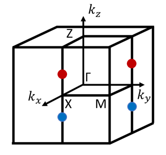
Figure 4: The position of the Dirac points in the noninteracting limit. The red (blue) indicates a positive (negative) sign of monopole charge (defined for spin-$\uparrow$ component).

Appendix C Details of the cluster slave spin calculation

In this section, we describe the cluster SS method. As we consider only the interactions on the heavy orbitals, the physical fermionic operators of the heavy orbitals are expressed in terms of the SS and spinon operators as $\psi_{\tau h\sigma}^{\dagger}=S^{+}_{\tau h\sigma}f_{\tau h\sigma}^{\dagger}$. The intra-orbital Hubbard interaction can be represented by the SS operators as:

$$\mathcal{H}_{int}=\frac{U}{2}\sum_{i,\tau}\left(\sum_{\sigma}S^{z}_{\tau h\sigma}\right)^{2}\,.$$ (12)

This representation has a U(1) symmetry. Compared to the $Z_{2}$ formulation de’Medici et al. (2005), it has the advantage of allowing the charge degrees of freedom to be expressed in terms of the SS operators alone. Finally, compared to the cluster formulation Yu et al. (2011); Zhao and Paramekanti (2007) of the slave rotor approach Florens and Georges (2004); Ding et al. (2019), the small Hilbert space of a slave spin operator facilitates the analysis of the cluster equations.

We then treat the full Hamiltonian at the saddle point level, which contains two decomposed effective Hamiltonian with the SS and spinon operactors only. They are specified as follows,

$$\mathcal{H}^{f} =\sum_{\begin{subarray}{c}ij,\sigma,\tau\tau^{\prime}\end{subarray}}t_{\tau\tau^{\prime}}^{h}e^{i\theta_{ij,h\sigma}^{\tau\tau^{\prime}}}\langle S^{+}_{i\tau h\sigma}S^{-}_{j\tau^{\prime}h\sigma}\rangle f_{i\tau h\sigma}^{\dagger}f_{j\tau^{\prime}h\sigma}+h.c.+\sum_{\begin{subarray}{c}ij,\sigma,\tau\tau^{\prime}\end{subarray}}t_{hl}\langle S_{i\tau h\sigma}^{+}\rangle f_{i\tau h\sigma}^{\dagger}\psi_{j\tau^{\prime}l\sigma}+h.c.$$ (13)

$$-\lambda\sum_{i\sigma,\tau}f_{i\tau h\sigma}^{\dagger}f_{i\tau h\sigma}+\mathcal{H}[\psi_{Al},\psi_{Bl}]\,,$$

$$\mathcal{H}^{S} =\sum_{\begin{subarray}{c}ij\sigma,\tau\tau^{\prime}\end{subarray}}t_{\tau\tau^{\prime}}^{h}\langle e^{i\theta_{ij,h\sigma}^{\tau\tau^{\prime}}}f_{i\tau h\sigma}^{\dagger}f_{j\tau^{\prime}h\sigma}\rangle S^{+}_{i\tau h\sigma}S^{-}_{j\tau^{\prime}h\sigma}+h.c.+\sum_{\begin{subarray}{c}ij\sigma,\tau\tau^{\prime}\end{subarray}}t_{hl}\langle f_{i\tau h\sigma}^{\dagger}\psi_{j\tau^{\prime}l\sigma}\rangle S_{i\tau h\sigma}^{+}+h.c.$$ (14)

$$+\lambda\sum_{i\sigma,\tau}\left(S^{z}_{i\tau h\sigma}+\frac{1}{2}\right)+\mathcal{H}_{int}\,,$$

where $\theta^{\tau\tau^{\prime}}_{ij,h\sigma}$ is the phase factor between the sublattices $\tau$ and $\tau^{\prime}$ of the heavy orbitals in unit cells $i$ and $j$ for spin $\sigma$, and $t_{AA}^{h}=-t_{BB}^{h}=t_{h}$, $t_{AB}^{h}=t_{BA}^{h}=t^{soc}_{h}$. $\mathcal{H}[\psi_{Al},\psi_{Bl}]$ is the noninteracting Hamiltonian between the light orbitals. A Lagrangian multiplier $\lambda$ is introduced to fix the constraint $S^{z}_{i\tau h\sigma}+1/2=f^{\dagger}_{i\tau h\sigma}f_{i\tau h\sigma}$. Similar to the cluster formulations of other auxiliary-particle approaches Yu et al. (2011); Zhao and Paramekanti (2007), we treat the SS Hamiltonian by considering a cluster with two unit cells embedded in an average medium. This leads to a cluster SS Hamiltonian

$$\mathcal{H}^{S} =\sum_{\tau}t_{\tau\tau}^{h}\chi^{\tau\tau}_{S}S^{+}_{\tau h\sigma,1}S^{-}_{\tau h\sigma,2}+h.c.+\sum_{\begin{subarray}{c}\tau\tau^{\prime},\tau\neq\tau^{\prime}\end{subarray}}t_{\tau\tau^{\prime}}^{h}\chi^{\tau\tau^{\prime}}_{S}S^{+}_{\tau h\sigma,1}S^{-}_{\tau^{\prime}h\sigma,2}+h.c.$$ (15)

$$+\sum_{\tau}5t_{\tau\tau}^{h}\chi_{S}^{\tau\tau}\langle S_{\tau h\sigma}^{+}\rangle\left(S^{-}_{\tau h\sigma,1}+S^{-}_{\tau h\sigma,2}\right)+h.c.+\sum_{\begin{subarray}{c}\tau\tau^{\prime},\tau\neq\tau^{\prime}\end{subarray}}3t_{\tau\tau^{\prime}}^{h}\chi^{\tau\tau^{\prime}}_{S}\langle S_{\tau h\sigma}^{+}\rangle\left(S^{-}_{\tau^{\prime}h\sigma,1}+S^{-}_{\tau^{\prime}h\sigma,2}\right)+h.c.$$

$$+\sum_{\begin{subarray}{c}\sigma,\tau\tau^{\prime}\end{subarray}}6t_{hl}\chi^{f_{\tau}\psi_{\tau^{\prime}}}_{S}\left(S^{+}_{\tau h\sigma,1}+S^{+}_{\tau h\sigma,2}\right)+h.c.+\lambda\sum_{\sigma,\tau}\left(S^{z}_{\tau h\sigma,1}+S^{z}_{\tau h\sigma,2}+1\right)+\mathcal{H}_{int}\,,$$

where the subscripts $1,2$ label the two unit cells in the cluster, and

$$\chi^{\tau\tau}_{S} =\frac{1}{12N_{\bm{k}}}\sum_{\bm{k}}\epsilon_{\bm{k}}\langle f_{\bm{k}\tau h\sigma}^{\dagger}f_{\bm{k}\tau h\sigma}\rangle\,,$$ (16)

$$\chi^{\tau\tau^{\prime}}_{S} =\frac{1}{8N_{k}}\sum_{\bm{k}}V_{\bm{k}}\langle f^{\dagger}_{\bm{k}\tau h\sigma}f_{\bm{k}\tau^{\prime}h\sigma}\rangle\,,$$

$$\chi^{f_{\tau}\psi_{\tau^{\prime}}}_{S} =\frac{1}{12N_{k}}\sum_{\bm{k}}\epsilon_{k}\langle f^{\dagger}_{\bm{k}\tau h\sigma}\psi_{\bm{k}\tau^{\prime}l\sigma}\rangle\,.$$

The expectation values appearing in the $\mathcal{H}^{f}$ are then replaced by the expectation values obtained from $\mathcal{H}^{S}$ of Eq. (15):

$$\langle S^{+}_{i\tau h\sigma}S^{-}_{j\tau^{\prime}h\sigma}\rangle=\begin{cases}\langle S_{\tau h\sigma,1}^{+}S^{-}_{\tau^{\prime}h\sigma,2}\rangle&i,j\in n.n.\\ 0&otherwise\end{cases}$$ (17)

$$\langle S^{+}_{i\tau h\sigma}\rangle=\langle S^{+}_{\tau h\sigma,1}\rangle=\langle S^{+}_{\tau h\sigma,2}\rangle=\sqrt{Z_{\tau h\sigma}}\,.$$ (18)

The spinon Hamiltonian is then written as

$$\mathcal{H}^{f} =\sum_{ij\sigma,\tau}t_{\tau\tau}^{h}\chi^{1}_{f}f^{\dagger}_{i\tau h\sigma}f_{j\tau h\sigma}+h.c.+\sum_{\begin{subarray}{c}ij\sigma,\tau\tau^{\prime},\tau\neq\tau^{\prime}\end{subarray}}t_{\tau\tau^{\prime}}^{h}\chi^{2}_{f}f_{i\tau h\sigma}^{\dagger}f_{j\tau h\sigma}+h.c.$$ (19)

$$+\sum_{\begin{subarray}{c}ij\sigma,\tau\tau^{\prime}\end{subarray}}t_{hl}\sqrt{Z_{i\tau h\sigma}}f^{\dagger}_{i\tau h\sigma}\psi_{j\tau^{\prime}l\sigma}+h.c.-\lambda\sum_{i\sigma,\tau}f_{i\tau h\sigma}^{\dagger}f_{i\tau h\sigma}+\mathcal{H}[\psi_{Al},\psi_{Bl}],$$

with $\chi_{f}^{1}=\langle S^{+}_{Ah\sigma,1}S^{-}_{Ah\sigma,2}\rangle$ and $\chi_{f}^{2}=\langle S^{+}_{Ah\sigma,1}S^{-}_{Bh\sigma,2}\rangle$. Combining the equations from Eq. (15)-(19), it is sufficient to solve the interacting Hamiltonian self-consistently. The variance of $\chi^{1}_{f}$, $\chi^{2}_{f}$ and quasipartice weight is shown in Fig. 5. Both $\chi^{1}_{f}$ and $\chi^{2}_{f}$ remain to be nonzero throughout, while $Z=0$ in the OSMP. We note that the filling of each orbital remains $1$ throughout the phase diagram.

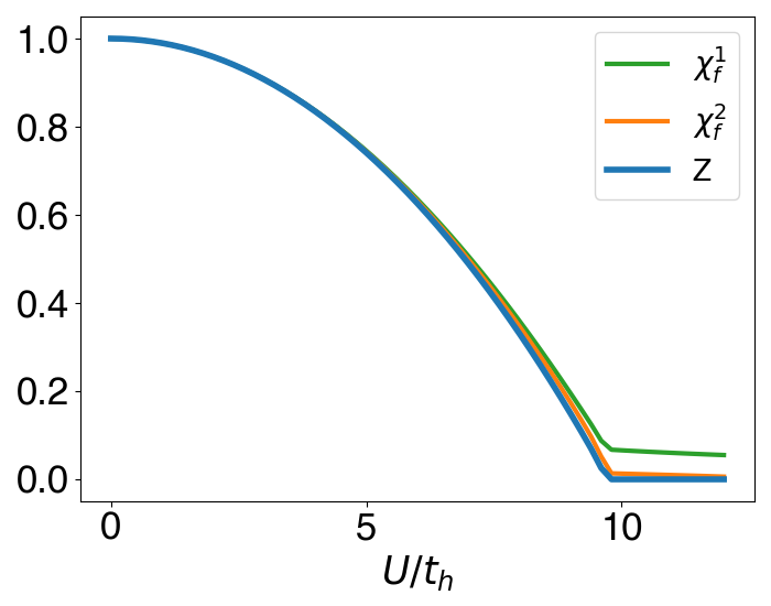
Figure 5: The quasiparticle weight and the expectation values of the bond operators $\chi_{f}^{1}$ and $\chi_{f}^{2}$ versus the interaction strength.

Appendix D Single-particle Green’s function in the cluster slave spin method

The cluster SS method gives rise to a translationally-invariant single-particle Green’s function of physical electrons. It is obtained by

$$G_{\psi}^{\tau\tau^{\prime}}(\bm{k},\omega) =\sum_{\bm{R}}e^{-i\bm{k}\bm{R}}G_{\psi}^{\tau\tau^{\prime}}(\bm{R},\omega)$$ (20)

$$=G_{\psi}^{\tau\tau^{\prime}}(\bm{0},\omega)+\sum_{\bm{R}\neq\bm{0}}e^{-i\bm{k}\bm{R}}G_{\psi}^{\tau\tau^{\prime}}(\bm{R},\omega),$$

where the spin and orbital indices are abbreviated. At zero temperature, the first term is calculated by

$$G_{\psi}^{\tau\tau^{\prime}}(\bm{0},\omega)=\sum_{\bm{k}}\sum_{\alpha}\sum_{m}\Lambda_{\tau\tau^{\prime}}^{\alpha,\bm{k}}\left[\frac{\langle 0|S^{+}_{\tau,1}|m\rangle\langle m|S^{-}_{\tau^{\prime},1}|0\rangle\left(1-\Theta(\epsilon_{\bm{k}}^{\alpha})\right)}{\omega-E_{m}-\epsilon^{\alpha}_{\bm{k}}}+\frac{\langle 0|S^{-}_{\tau^{\prime},1}|m\rangle\langle m|S^{+}_{\tau,1}|0\rangle\Theta(\epsilon_{\bm{k}}^{\alpha})}{\omega+E_{m}-\epsilon^{\alpha}_{\bm{k}}}\right],$$ (21)

where $\Lambda_{\tau\tau^{\prime}}^{\alpha,\bm{k}}=\langle\alpha_{\bm{k}}|f^{\dagger}_{\bm{k}\tau}f_{\bm{k}\tau^{\prime}}|\alpha_{\bm{k}}\rangle$, with $\epsilon_{\bm{k}}^{\alpha}$ ($|\alpha_{\bm{k}}\rangle$) the $\alpha$-th eigenvalues (eigenvectors) of the spinon Hamiltonian. Here, $|m\rangle$ enumerates the eigenvectors of the cluster SS Hamiltonian (Eq. (15)) and $E_{m}$ denotes the corresponding eigen-energy. The second term can be obtained from:

$$G_{\psi}^{\tau\tau^{\prime}}(\bm{R},\omega)=\sum_{\bm{k}}\sum_{\alpha}\sum_{m}e^{i\bm{k}\bm{R}}\Lambda_{\tau\tau^{\prime}}^{\alpha,\bm{k}}\left[\frac{\langle 0|S^{+}_{\tau,1}|m\rangle\langle m|S^{-}_{\tau^{\prime},2}|0\rangle\left(1-\Theta(\epsilon_{\bm{k}}^{\alpha})\right)}{\omega-E_{m}-\epsilon^{\alpha}_{\bm{k}}}+\frac{\langle 0|S^{-}_{\tau^{\prime},2}|m\rangle\langle m|S^{+}_{\tau,1}|0\rangle\Theta(\epsilon_{\bm{k}}^{\alpha})}{\omega+E_{m}-\epsilon^{\alpha}_{\bm{k}}}\right],$$ (22)

where the operator $S^{\pm}_{\tau,1}$ and $S^{\pm}_{\tau,2}$ are sitting on different unit cells in the SS cluster. The translational invariance of the Green’s function is satisfied because all the sites and bonds pick up the SS contributions according to Eqs. (17) and (18).

These two terms can be further separated into coherent and incoherent parts. The coherent part, associated directly with the quasiparticles weights as described by the first term in Eq. (3), is obtained from Eq. (20)-(22) with $m=0$. The incoherent part, on the other hand, is obtained from Eq. (20)-(22) by summing up terms with $m\neq 0$.

References

- Keimer and Moore (2017) B. Keimer and J. E. Moore, Nat. Phys. 13, 1045 (2017).
- Paschen and Si (2021) S. Paschen and Q. Si, Nat. Rev. Phys. 3, 9 (2021).
- Stormer et al. (1999) H. L. Stormer, D. C. Tsui, and A. C. Gossard, Rev. Mod. Phys. 71, S298 (1999).
- Xie et al. (2021) Y. Xie, A. T. Pierce, J. M. Park, D. E. Parker, E. Khalaf, P. Ledwith, Y. Cao, S. H. Lee, S. Chen, P. R. Forrester, K. Watanabe, T. Taniguchi, A. Vishwanath, P. Jarillo-Herrero, and A. Yacoby, Nature 600, 439 (2021).
- Zeng et al. (2023) Y. Zeng, Z. Xia, K. Kang, J. Zhu, P. Knüppel, C. Vaswani, K. Watanabe, T. Taniguchi, K. F. Mak, and J. Shan, Nature 622, 69 (2023).
- Lu et al. (2023) Z. Lu, T. Han, Y. Yao, A. P. Reddy, J. Yang, J. Seo, K. Watanabe, T. Taniguchi, L. Fu, and L. Ju, arXiv preprint arXiv:2309.17436 (2023).
- Lai et al. (2018) H.-H. Lai, S. E. Grefe, S. Paschen, and Q. Si, Proc. Natl. Acad. Sci. U.S.A. 115, 93 (2018).
- Dzsaber et al. (2017) S. Dzsaber, L. Prochaska, A. Sidorenko, G. Eguchi, R. Svagera, M. Waas, A. Prokofiev, Q. Si, and S. Paschen, Phys. Rev. Lett. 118, 246601 (2017).
- Dzsaber et al. (2021) S. Dzsaber, X. Yan, M. Taupin, G. Eguchi, A. Prokofiev, T. Shiroka, P. Blaha, O. Rubel, S. E. Grefe, H.-H. Lai, Q. Si, and S. Paschen, Proc. Natl. Acad. Sci. U.S.A. 118, e2013386118 (2021).
- Chen et al. (2022) L. Chen, C. Setty, H. Hu, M. G. Vergniory, S. E. Grefe, L. Fischer, X. Yan, G. Eguchi, A. Prokofiev, S. Paschen, J. Cano, and Q. Si, Nat. Phys. 18, 134101346 (2022).
- Armitage et al. (2018) N. P. Armitage, E. J. Mele, and A. Vishwanath, Rev. Mod. Phys. 90, 015001 (2018).
- Nagaosa et al. (2020) N. Nagaosa, T. Morimoto, and Y. Tokura, Nature Reviews Materials 5, 621 (2020).
- Bradlyn et al. (2017) B. Bradlyn, L. Elcoro, J. Cano, M. G. Vergniory, Z. Wang, C. Felser, M. I. Aroyo, and B. A. Bernevig, Nature 547, 298 (2017).
- Cano et al. (2018) J. Cano, B. Bradlyn, Z. Wang, L. Elcoro, M. G. Vergniory, C. Felser, M. I. Aroyo, and B. A. Bernevig, Phys. Rev. B 97, 035139 (2018).
- Po et al. (2017) H. C. Po, A. Vishwanath, and H. Watanabe, Nature Communications 8, 50 (2017).
- Watanabe et al. (2016) H. Watanabe, H. C. Po, M. P. Zaletel, and A. Vishwanath, Phys. Rev. Lett. 117, 096404 (2016).
- Cano and Bradlyn (2021) J. Cano and B. Bradlyn, Annu. Rev. Condens. Matter Phys. 12, 225 (2021).
- Abrikosov et al. (2012) A. A. Abrikosov, L. P. Gorkov, and I. E. Dzyaloshinski, Methods of quantum field theory in statistical physics (Courier Corporation, 2012).
- Hu et al. (2021) H. Hu, L. Chen, C. Setty, S. E. Grefe, A. Prokofiev, S. Kirchner, S. Paschen, J. Cano, and Q. Si, arXiv preprint arXiv:2110.06182 (2021).
- Setty et al. (2023a) C. Setty, F. Xie, S. Sur, L. Chen, S. Paschen, M. G. Vergniory, J. Cano, and Q. Si, arXiv preprint arXiv:2311.12031 (2023a).
- Dzyaloshinskii (2003) I. Dzyaloshinskii, Phys. Rev. B 68, 085113 (2003).
- Essin and Gurarie (2011) A. M. Essin and V. Gurarie, Phys. Rev. B 84, 125132 (2011).
- You et al. (2018) Y.-Z. You, Y.-C. He, C. Xu, and A. Vishwanath, Phys. Rev. X 8, 011026 (2018).
- Setty et al. (2023b) C. Setty, S. Sur, L. Chen, F. Xie, H. Hu, S. Paschen, J. Cano, and Q. Si, arXiv preprint arXiv:2301.13870 (2023b).
- Wagner et al. (2023a) N. Wagner, L. Crippa, A. Amaricci, P. Hansmann, M. Klett, E. J. König, T. Schäfer, D. D. Sante, J. Cano, A. J. Millis, A. Georges, and G. Sangiovanni, Nature Communications 14, 7531 (2023a).
- Morimoto and Nagaosa (2016) T. Morimoto and N. Nagaosa, Sci. Rep. 6, 19853 (2016).
- Kirchner et al. (2020) S. Kirchner, S. Paschen, Q. Chen, S. Wirth, D. Feng, J. D. Thompson, and Q. Si, Rev. Mod. Phys. 92, 011002 (2020).
- Si et al. (2001) Q. Si, S. Rabello, K. Ingersent, and J. Smith, Nature 413, 804 (2001).
- Coleman et al. (2001) P. Coleman, C. Pépin, Q. Si, and R. Ramazashvili, J. Phys.: Condens. Matter 13, R723 (2001).
- Senthil et al. (2004) T. Senthil, M. Vojta, and S. Sachdev, Phys. Rev. B 69, 035111 (2004).
- Anisimov et al. (2002) V. Anisimov, I. Nekrasov, D. Kondakov, T. Rice, and M. Sigrist, The European Physical Journal B-Condensed Matter and Complex Systems 25, 191 (2002).
- Yi et al. (2017) M. Yi, Y. Zhang, Z.-X. Shen, and D. Lu, npj Quantum Mater. 2, 57 (2017).
- Si and Hussey (2023) Q. Si and N. E. Hussey, Phys. Today 76, 34 (2023).
- Zhao et al. (2023a) W. Zhao, B. Shen, Z. Tao, Z. Han, K. Kang, K. Watanabe, T. Taniguchi, K. F. Mak, and J. Shan, Nature 616, 61 (2023a).
- Guerci et al. (2023) D. Guerci, J. Wang, J. Zang, J. Cano, J. H. Pixley, and A. Millis, Sci. Adv. 9, eade7701 (2023).
- Xie et al. (2023) F. Xie, L. Chen, and Q. Si, arXiv preprint arXiv:2310.20676 (2023).
- Zhao et al. (2023b) W. Zhao, B. Shen, Z. Tao, S. Kim, P. Knüppel, Z. Han, Y. Zhang, K. Watanabe, T. Taniguchi, D. Chowdhury, J. Shan, and K. F. Mak, arXiv preprint arXiv:2310.06044 (2023b).
- Hu and Si (2023) H. Hu and Q. Si, Sci. Adv. 9, eadg0028 (2023).
- (39) J. Huang, C. Setty, L. Deng, J.-Y. You, H. Liu, S. Shao, J. S. Oh, Y. Guo, Y. Zhang, Z. Yue, J.-X. Yin, M. Hashimoto, D. Lu, S. Gorovikov, P. Dai, M. Z. Hasan, Y.-P. Feng, R. J. Birgeneau, Y. Shi, C.-W. Chu, G. Chang, Q. Si, and M. Yi, “Three-dimensional flat bands and Dirac cones in a pyrochlore superconductor, To appear in Nat. Phys., arXiv:2304.09066 (2023),” .
- Yu and Si (2012) R. Yu and Q. Si, Phys. Rev. B 86, 085104 (2012).
- Yu and Si (2017) R. Yu and Q. Si, Phys. Rev. B 96, 125110 (2017).
- Komijani and Kotliar (2017) Y. Komijani and G. Kotliar, Phys. Rev. B 96, 125111 (2017).
- Seki and Yunoki (2017) K. Seki and S. Yunoki, Phys. Rev. B 96, 085124 (2017).
- Setty et al. (2023c) C. Setty, F. Xie, S. Sur, L. Chen, M. G. Vergniory, and Q. Si, arXiv preprint arXiv:2309.14340 (2023c).
- Blason and Fabrizio (2023) A. Blason and M. Fabrizio, Phys. Rev. B 108, 125115 (2023).
- Peralta Gavensky et al. (2023) L. Peralta Gavensky, S. Sachdev, and N. Goldman, Phys. Rev. Lett. 131, 236601 (2023).
- Zhao et al. (2023c) J. Zhao, P. Mai, B. Bradlyn, and P. Phillips, Phys. Rev. Lett. 131, 106601 (2023c).
- Fabrizio (2022) M. Fabrizio, Nature Communications 13, 1 (2022).
- Wagner et al. (2023b) N. Wagner, D. Guerci, A. J. Millis, and G. Sangiovanni, arXiv preprint arXiv:2312.13226 (2023b).
- Bollmann et al. (2023) S. Bollmann, C. Setty, U. F. Seifert, and E. J. König, arXiv preprint arXiv:2312.14926 (2023).
- Yang et al. (2015) B.-J. Yang, T. Morimoto, and A. Furusaki, Phys. Rev. B 92, 165120 (2015).
- de’Medici et al. (2005) L. de’Medici, A. Georges, and S. Biermann, Phys. Rev. B 72, 205124 (2005).
- Yu et al. (2011) R. Yu, J.-X. Zhu, and Q. Si, Phys. Rev. Lett. 106, 186401 (2011).
- Zhao and Paramekanti (2007) E. Zhao and A. Paramekanti, Phys. Rev. B 76, 195101 (2007).
- Florens and Georges (2004) S. Florens and A. Georges, Phys. Rev. B 70, 035114 (2004).
- Ding et al. (2019) W. Ding, R. Yu, Q. Si, and E. Abrahams, Phys. Rev. B 100, 235113 (2019).