Superfluidity of indirect momentum space dark dipolar excitons in a double layer with massive anisotropic tilted semi-Dirac bands

Abstract

We have theoretically investigated the spin- and valley-dependent superfluidity properties of indirect momentum space dark dipolar excitons in double layers with massive anisotropic tilted semi-Dirac bands in the presence of circularly polarized irradiation. An external vertical electric field is also applied to the structure and is responsible for tilting and gap opening for the band structure. For our calculations we used the parameters of a double layer of 1T^′-MoS₂. Closed form analytical expressions are presented for the energy spectrum for excitons, their associated wave functions and binding energies. Additionally, we examine the effects which the intensity and frequency of circularly polarized irradiation has for 1T^′-MoS₂ on the effective mass of the excitons since it has been demonstrated that the application of an external high-frequency dressing field tailors the crucial electronic including the exciton binding energy, as well as the critical temperature for superfluidity. We also calculate the sound velocity in the anisotropic weakly-interacting Bose gas of two-component indirect momentum space dark excitons for a double layer of 1T^′-MoS₂. We show that the critical velocity of superfluidity, the spectrum of collective excitations, concentrations of the superfluid and normal component, and mean field critical temperature for superfluidity are anisotropic and formed by a two-component system. The critical temperature for superfluidity is increased when the exciton concentration and interlayer separation are increased. We propose the use of phonon-assisted photoluminescence to experimentally confirm directional superfluidity of indirect momentum space dark excitons in a double layer with massive anisotropic tilted semi-Dirac bands.

I Introduction

Transition metal dichalcogenides (TMDCs) have been gaining much attention in recent times for their remarkable optoelectronic as well as transport properties. TMDCs have been found to have applications for a range of fundamental phenomena optoElectronics . These materials can can sustain the formation of polaritons at room temperature due to their relatively larger binding energy starkEffect . Indirect momentum space dark excitons in a monolayer with massive anisotropic tilted semi-Dirac bands have been the subject of recent experimental studies GrossPoster ; OpticalReadout ; StrainExciton . So far, massive anisotropic tilted Dirac systems such as 1T^′-MoS₂ are one of the more interesting 2D Dirac materials, due to their thermodynamic stability and their ease of synthesis in the semiconducting phase. 1T^′-MoS₂ has been predicted to display a strong quantum-spin Hall effect TiltedCones . When a uniform perpendicular external electric field is applied, it exhibits valley-spin polarized Dirac bands BGR as well as a phase transition between topological insulator and regular band insulator aniso1T . The anisotropy of the energy band structure is consequential due to its tilted and shifted valence and conduction Dirac bands TMDCsAbstract .

Bose-Einstein condensation (BEC) occurs when bosons at low temperatures occupy the lowest energy quantum state. Due to the relatively large exciton binding energies in 2D semiconductors, such as 1T^′-MoS₂, BEC and superfluidity of dipolar excitons in double layer 1T^′-MoS₂ are possible. Since the de Broglie wavelength for a 2D system is inversely proportional to the square root of the mass of a particle, BEC is more likely to exist for bosons of larger mass at higher temperatures than for bosons with smaller mass. A BEC of weakly interacting particles was famously achieved experimentally in dilute gas of alkali atoms, albeit at challenglingly low temperatures in the nano Kelvin scale regime Nobel . Therefore, BEC exists at much higher temperatures in a Bose gas consisting of particles whose mass is smaller than those in a system of relatively heavy alkali atoms. The BEC and superfluidity of dipolar bright excitons was predicted for double layers in Ref. LYGroundState and discussed for the double layers of TMDCs in Refs. Butov ; HighTempSuperOleg ; SuperfluidDipolar .

The BEC and superfluidity of dipolar indirect momentum space excitons are intriguing due to the fact that we expect that such excitons will be characterized by the higher lifetime than regular dipolar excitons, since their recombination with the photon emission is forbidden by selection rules Lifetime .

In this paper, we develop an approach to study the superfluidity of a two-component dilute Bose gas of dipolar excitons in a double layer of massive anisotropic tilted Dirac systems. While we perform our calculations for the specific case the double layer of tilted 1T^′-MoS₂, our approach can be applied to other massive anisotropic tilted Dirac systems without loss of generality. We investigate three different types of excitons. These are based on their spin and valley polarizations as well as the way in which they alter the effective masses and center-of-masses of the excitons. We also study the effect which chosen parameters have on the binding energy of the three different types of excitons. Specifically, we analyze the way in which varying the relative value of the perpendicular electric field affects the binding energy. From this, we gain insight regarding the use of a number of dielectric layers (in our case hexagonal boron nitride, h-bN), for experimental exploration and their associated effects Rubio .

The rest of this paper is organized as follows. In Sec.  II, the two-body problem for an electron and a hole, spatially separated in two parallel monolayers of 1T^′-MoS₂, is formulated. The wave function and binding energy for a single dipolar exciton in the 1T^′-MoS₂ double layer are calculated. Section  III is devoted to studying whether the electron-photon dressed states by circularly polarized light, predicted in Ref. Floquet , allow for sufficient modification of the binding energy by changing the irradiation intensity and frequency of the dressing field. In Sec. IV, we study the formation of collective excitations for spatially separated electrons and holes. In Sec.  V, we turn our attention to the case of two-component superfluidity exhibiting directionality induced by anisotropy of the system, for the soundlike spectrum of collective excitations, and the dependence of the sound velocity and critical temperature on the angle $\Theta$, a parameter which transforms the center-of-mass momentum into polar coordinates. Section  VI discusses our results obtained for or the superfluidity. We propose a way to experimentally observe the indirect-momentum space dark excitons and related phenomena. Section  VII contains our concluding remarks.

II The interacting electron-hole pair

We begin by computing the wavefunctions and energy eigenvalues of the massive anisotropic tilted Dirac systems by examining the general Hamiltonian GenHamiltonian . By examining the energy dispersion relation, and modifying it to the form of the model Hamiltonian for $\mathrm{1T^{\prime}-MoS_{2}}$ with tilted Dirac bands, we are able to solve exactly for the analytical solution of the system. The model Hamiltonian within the effective mass approximation for a single electron-hole pair in a $\mathrm{1T^{\prime}-MoS_{2}}$ double layer is given by BGR

$$\hat{H}_{0}=-\frac{\hbar^{2}}{2m_{x}^{e}}\frac{\partial^{2}}{\partial x_{1}^{2}}-\frac{\hbar^{2}}{2m_{y}^{e}}\left[\frac{\partial}{\partial y_{1}}-p_{e}^{(0)}\right]^{2}-\frac{\hbar^{2}}{2m_{x}^{h}}\frac{\partial^{2}}{\partial x_{2}^{2}}-\frac{\hbar^{2}}{2m_{y}^{h}}\left[\frac{\partial}{\partial y_{2}}-p_{h}^{(0)}\right]^{2}+V\left(\sqrt{r^{2}+D^{2}}\right)\ ,$$ (1)

where $V\left(\sqrt{r^{2}+D^{2}}\right)$ is the potential energy for electron-hole pair attraction, when the electron and hole are located in two parallel monolayers separated by distance $D$. The Hamiltonian reflects the anisotropy of the system. In Eq. (1), $m_{x}^{e}$, $m_{y}^{e}$, $m_{x}^{h}$, $m_{y}^{h}$, $p_{e}^{(0)}$, and $p_{h}^{(0)}$ are effective constants which can be obtained from Eq. (A.2) using the method of completing squares as seen below. The constants $m_{x}^{e}$, $m_{y}^{e}$, $m_{x}^{h}$, and $m_{y}^{h}$ are the effective masses of the electrons and holes in $x$ and $y$. The constants $p_{e}^{(0)}$, and $p_{h}^{(0)}$ are effective constants that reflect the anisotropy of the band structure.

$$E(k)=E_{0}+\frac{\hbar^{2}}{2m^{*}_{x}}(k_{x}-k_{0,x})^{2}+\frac{\hbar^{2}}{2m^{*}_{y}}(k_{y}-k_{0,y})^{2}$$ (2)

For the energy spectrum of Eq.(2) the method of completing the square is outlined below

$$\epsilon_{\xi,s}^{\lambda}({\bf k})=\xi|\lambda-s\alpha|\Delta+\left(\dfrac{\xi v_{+}^{2}\hbar^{2}}{2\Delta|\lambda-\alpha s|}\right)\left({k_{y}}^{2}+\frac{\left[-\lambda\hbar v_{-}+\xi\hbar v_{2}\ \text{sgn}(\lambda-s\alpha)\right]({2\Delta|\lambda-\alpha s|})}{{\xi v_{+}^{2}\hbar^{2}}}k_{y}\right)+\left(\dfrac{\xi v_{1}^{2}\hbar^{2}}{2\Delta|\lambda-\alpha s|}\right)\left(k_{x}^{2}\right)$$ (3)

We visualise the energy bands as a function of $k_{x}$ and $k_{y}$ for the different excitons outlined thoroughly in Section II.B, which differ by the choice of spin and valley.

(

(

(

(

(

(

Figure 1: (Color online) Visualization of the energy dispersion bands for the charge carriers, forming the different types of excitons explored in this paper, with different values of $\alpha$ - (a) Type A excitons with $\alpha=0.1$, (b) Type A excitons with $\alpha=0.5$, (c) Type B excitons with $\alpha=0.1$, (d) Type B excitons with $\alpha=0.5$, (e) Type C excitons with $\alpha=0.1$, and (f) Type C excitons with $\alpha=0.5$.

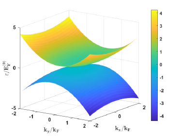
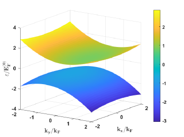
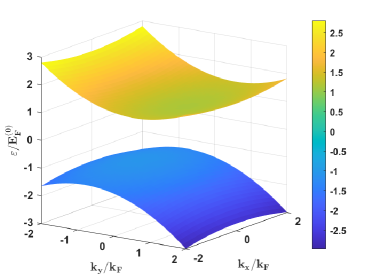
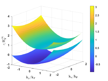
a) b) c) d) e) f)

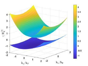
The bands do not form full Dirac cones but rather semi-Dirac cones. Visualisation of the energy dispersion bands for the charge carriers, forming each of the different types of excitons is presented in Fig.1 The difference in band curvature at the origin between different types of excitons leads to the fact that different types of excitons are characterized by different effective masses. The curvature also changes for different values of $\alpha$. We can find such value of $\alpha$, which will correspond to the higher exciton binding energy implying more stable excitons. Fig.1 also demonstrates the anisotropy of our system, which forms the basis for the directional indirect momentum space dark exciton superfluidity presented in Secs. VI-VII.

From Eq. (3) we can infer the expressions for the effective constants.

$$m_{x}^{e/h}=\dfrac{\Delta|\lambda-\alpha s|}{\xi v_{1}^{2}},\hskip 14.22636ptm_{y}^{e/h}=\dfrac{\Delta|\lambda-\alpha s|}{\xi v_{+}^{2}}$$ (4)

$$p_{e/h}^{(0)}=\frac{-{i}\left[-\lambda\hbar v_{-}+\xi\hbar v_{2}\ \text{sgn}(\lambda-s\alpha)\right]({\Delta|\lambda-\alpha s|})}{{\xi v_{+}^{2}\hbar^{2}}},\hskip 14.22636pt\tilde{p}_{e/h}^{(0)}=\frac{\left[-\lambda\hbar v_{-}+\xi\hbar v_{2}\ \text{sgn}(\lambda-s\alpha)\right]({\Delta|\lambda-\alpha s|})}{{\xi v_{+}^{2}\hbar^{2}}}$$ (5)

It is worth noting that $p_{e/h}^{(0)}$ is a complex number, and as such the real valued constant $\tilde{p}_{e/h}^{(0)}$ was introduced, where $p_{e/h}^{(0)}=-{i}\hskip 1.42271pt\tilde{p}_{e/h}^{(0)}$, to easily identify complex numbers in differential equations. An extra energy term arises as a constant from Eq.(A.2). Following the procedure LandauStat ; Prada for the separation of the relative motion of the electron-hole pair from their center-of-mass motion one can introduce variables for the center-of-mass of an electron-hole pair $\mathbf{R}=(X,Y)$ and the relative motion of an electron and a hole $\mathbf{r}=(x,y)$, $X=(m_{x}^{e}x_{1}+m_{x}^{h}x_{2})/(m_{x}^{e}+m_{x}^{h})$,  $Y=(m_{y}^{e}y_{1}+m_{y}^{h}y_{2})/(m_{y}^{e}+m_{y}^{h})$,   $x=x_{1}-x_{2}\ ,y=y_{1}-y_{2}$ , and $r^{2}=x^{2}+y^{2}$.

The Schrödinger equation with Hamiltonian (1) has the form: $\hat{H}_{0}\Psi(\mathbf{r}_{1},\mathbf{r}_{2})=E\Psi(\mathbf{r}_{1},\mathbf{r}_{2})$, where $\Psi(\mathbf{r}_{1},\mathbf{r}_{2})$ and $E$ are the eigenfunction and eigenenergy. One can write $\Psi(\mathbf{r}_{1},\mathbf{r}_{2})$ in the form $\Psi(\mathbf{r}_{1},\mathbf{r}_{2})=\Psi(\mathbf{R},\mathbf{r})=\varphi({R})\hskip 2.84544pt\varphi(\mathbf{r})$, where $\varphi(\mathbf{R})$ is the wave function for the center-of-mass and $\varphi(\mathbf{r})$ is the wave function for the electron-hole pair.

The wave function for the center of mass is given by the 2D Schrödinger equation:

$$\left[-\frac{\hbar^{2}}{2M_{x}}\frac{\partial^{2}}{\partial X^{2}}-\frac{\hbar^{2}}{2M_{y}}\frac{\partial^{2}}{\partial Y^{2}}-{i}\frac{\hbar^{2}}{M_{y}}(\tilde{p}_{e}^{(0)}+\tilde{p}_{h}^{(0)})\frac{\partial}{\partial Y}+E_{0}^{(e)}+E_{0}^{(h)}+\eta\right]\varphi(X,Y)=\varepsilon_{COM}\hskip 2.84544pt\varphi(X,Y),$$ (6)

In Eq.(10), $m_{x}^{e}$, $m_{y}^{e}$, $m_{x}^{h}$, $m_{y}^{h}$, $p_{e}^{(0)}$, and $p_{h}^{(0)}$ are defined in Eqs.(4)-(5) and the reduced masses are defined as follows

$$\mu_{x}=\frac{m^{e}_{x}m^{h}_{x}}{m^{e}_{x}+m^{h}_{x}},\hskip 17.07182pt\mu_{y}=\frac{m^{e}_{y}m^{h}_{y}}{m^{e}_{y}+m^{h}_{y}}$$ (7)

$$\mu^{*}_{y}=\frac{m^{e}_{y}m^{h}_{y}}{m^{e}_{y}p^{(0)}_{h}+m^{h}_{y}p^{(0)}_{e}},\hskip 17.07182pt\tilde{\mu}^{*}_{y}=\frac{m^{e}_{y}m^{h}_{y}}{m^{e}_{y}\tilde{p}^{(0)}_{h}+m^{h}_{y}\tilde{p}^{(0)}_{e}}$$ (8)

$$\eta=\frac{\hbar^{2}}{2}\frac{m^{e}_{y}{{\tilde{p}^{(0)}_{h}}{}^{2}}+m^{h}_{y}{{\tilde{p}^{(0)}_{e}}}{}^{2}}{m^{e}_{y}m^{h}_{y}}$$ (9)

It is worth noting that $\eta$ is a positive, real number and ${\mu}^{*}_{y}$ is a complex number. Consequently, we introduce the real valued constant $\tilde{\mu}^{*}_{y}$ to easily identify complex numbers in equations. The relationship between them is ${\mu}^{*}_{y}={i}\hskip 1.42271pt\tilde{\mu}^{*}_{y}$. The wave function for the relative motion of the electron-hole pair is given by the 2D Schrödinger equation:

$$\left[-\frac{\hbar^{2}}{2\mu_{x}}\frac{\partial^{2}}{\partial x^{2}}-\frac{\hbar^{2}}{2\mu_{y}}\frac{\partial^{2}}{\partial y^{2}}+\frac{\hbar^{2}}{\mu^{*}_{y}}\frac{\partial}{\partial y}+V\left(\sqrt{r^{2}+D^{2}}\right)\right]\varphi(x,y)=\varepsilon_{rel}\hskip 2.84544pt\varphi(x,y),$$ (10)

$$\left[-\frac{\hbar^{2}}{2\mu_{x}}\frac{\partial^{2}}{\partial x^{2}}-\frac{\hbar^{2}}{2\mu_{y}}\frac{\partial^{2}}{\partial y^{2}}-{i}\frac{\hbar^{2}}{\tilde{\mu}^{*}_{y}}\frac{\partial}{\partial y}+V\left(\sqrt{r^{2}+D^{2}}\right)\right]\varphi(x,y)=\varepsilon_{rel}\hskip 2.84544pt\varphi(x,y),$$ (11)

II.1 Wave function and binding energy of an exciton

Electron-hole interaction in a double layer is discussed in Appendix B. Substituting Eq. (B.1) with parameters in Eq. (B.2) for Coulomb potential, and using $r^{2}=x^{2}+y^{2}$, one obtains an equation which has the form of the Schrödinger equation for a 2D anisotropic harmonic oscillator. This allows us to carry out separation of variables to obtain two independent equations

$$-\frac{\hbar^{2}}{2\mu_{x}}\frac{\partial^{2}}{\partial x^{2}}\psi(x)+\gamma x^{2}\psi(x)=\left(\varepsilon_{x}+\frac{V_{0}}{2}\right)\psi(x)$$ (12)

$$-\frac{\hbar^{2}}{2\mu_{y}}\frac{\partial^{2}}{\partial y^{2}}\psi(y)+\frac{\hbar^{2}}{\mu^{*}_{y}}\frac{\partial}{\partial y}\psi(y)+\gamma y^{2}\psi(y)=\left(\varepsilon_{y}+\frac{V_{0}}{2}\right)\psi(y)$$ (13)

The wavefunction and eigenenergies of Eq.(12) are obtained simply since it is the well-studied solution to a 1D harmonic oscillator. The process for solving Eq.(13) is the following. First we assume that $\psi(y)$ has the form of two functions multiplied.

$$\psi(y)=f(y)\cdot g(y)$$ (14)

allowing us to rewrite Eq.(13) into the following form

$$a_{2}\hskip 1.42271ptg(y)\frac{\partial^{2}}{\partial y^{2}}f(y)+\left(2a_{2}\frac{\partial}{\partial y}g(y)+a_{1}g(y)\right)\frac{\partial}{\partial y}f(y)+\left(a_{2}\frac{\partial^{2}}{\partial y^{2}}g(y)+a_{1}\frac{\partial}{\partial y}g(y)+(\gamma y^{2}-E_{y})g(y)\right)f(y)=0\ ,$$ (15)

where

$$E_{y}=\varepsilon_{y}+\frac{V_{0}}{2},\hskip 5.69046pta_{2}=-\frac{\hbar^{2}}{2\mu_{y}},\hskip 5.69046pta_{1}=\frac{\hbar^{2}}{\mu_{y}^{*}}=-{i}\hskip 0.56917pt\tilde{a}_{1},\hskip 5.69046pt\tilde{a}_{1}=\hskip 1.13791pt\frac{\hbar^{2}}{\tilde{\mu}_{y}^{*}}$$ (16)

By imposing the condition that the coefficient of the first derivative of $f(y)$ in Eq.(15) must be equal to zero, we find the form of $g(y)$.

$$2a_{2}\frac{\partial}{\partial y}g(y)-{i}\hskip 1.13791pt\tilde{a}_{1}g(y)=0,\hskip 5.69046ptg(y)=Fe^{{i}\hskip 0.85355pt\frac{\tilde{a}_{1}y}{2a_{2}}}\ ,$$ (17)

where $F$ is an undetermined constant. Inserting our result from Eq.(17) into Eq.(15) we obtain an equation that determines $f(y)$. This equation is of the form of a 1D harmonic oscillator.

$$a_{2}\frac{\partial^{2}}{\partial{y}^{2}}f(y)+\gamma y^{2}f(y)=\left(E_{y}-\frac{\tilde{a}_{1}^{2}}{4a_{2}}\right)f(y)$$ (18)

Using the condition of normalization $\int_{-\infty}^{\infty}|\psi(y)|^{2}\,dy=1$ we find $F$ = 1. The normalized eigenfunctions for Eq. (12) and Eq.  (13) are given by

$$\psi_{n}(x)=\frac{1}{\pi^{1/4}a_{x}^{1/2}}\frac{1}{\sqrt{2^{n}n!}}e^{-x^{2}/(2a_{x}^{2})}H_{n}\left(\frac{x}{a_{x}}\right)$$ (19)

$$\psi_{m}(y)=e^{-{i}\frac{\mu_{y}y}{\tilde{\mu}_{y}^{*}}}\frac{1}{\pi^{1/4}a_{y}^{1/2}}\frac{1}{\sqrt{2^{m}m!}}e^{-y^{2}/(2a_{y}^{2})}H_{m}\left(\frac{y}{a_{y}}\right)$$ (20)

where $n=0,1,2,3...$ and $m=0,1,2,3...$ are the quantum numbers, $H_{n}(\frac{x}{a_{x}})$, and $H_{m}(\frac{y}{a_{y}})$ are Hermite polynomials, and $a_{x}=(\hbar/(\sqrt{2\mu_{x}\gamma})^{1/2}$ and $a_{y}=(\hbar/(\sqrt{2\mu_{y}\gamma})^{1/2}$. The overarching wavefunction for the relative motion of the electron-hole pair in Eq.(10) is thus given by $\psi_{n,m}(x,y)=\psi_{n}(x)\psi_{m}(y).$ The corresponding eigenenergies are

$$\varepsilon_{n}^{(x)}=-\frac{V_{0}}{2}+\hbar\sqrt{\frac{2\gamma}{\mu_{x}}}(n+1/2),\hskip 17.07182pt\varepsilon_{m}^{(y)}=-\frac{V_{0}}{2}+\hbar\sqrt{\frac{2\gamma}{\mu_{y}}}(m+1/2)-\tilde{\chi}$$ (21)

where the constant term at the end of Eq. (22) is given by $\tilde{\chi}=\frac{\hbar^{2}\mu_{y}}{2{{{\tilde{\mu}_{y}{}^{*}}}}^{2}}.$ The total eigenergy of the relative motion of the electron-hole pair can be expressed as

$$\varepsilon_{nm}=\varepsilon_{n}^{(x)}+\varepsilon_{m}^{(y)}$$ (22)

where $n=0,1,2,3....$ and $m=0,1,2,3....$

The variables $X$ and $Y$ in the Schrödinger equation for center of mass can be separated in Eq.(6) to obtain the following equations

$$\left[-\frac{\hbar^{2}}{2M_{x}}\frac{\partial^{2}}{\partial X^{2}}\right]\phi(X)=\varepsilon_{X}\hskip 2.84544pt\phi(X),$$ (23)

$$\left[-\frac{\hbar^{2}}{2M_{y}}\frac{\partial^{2}}{\partial Y^{2}}-{i}\hskip 0.56917pt\frac{\hbar^{2}}{M_{y}}(\tilde{p}_{e}^{(0)}+\tilde{p}_{h}^{(0)})\ \ \frac{\partial}{\partial Y}\right]\phi(Y)=\varepsilon_{Y}\hskip 2.84544pt\phi(Y),$$ (24)

where $M_{X}=m_{x}^{e}+m_{x}^{h}$, and $M_{Y}=m_{y}^{e}+m_{y}^{h}$. We will also be using the notation $\tau=\tilde{p}_{e}^{(0)}+\tilde{p}_{h}^{(0)}$ for convenience. The equation for the center of mass in $X$, Eq.(23), is simply that of a free particle. The solution of Eq.(23)-(24), $\phi(X)$ and $\phi(Y)$ is given by

$$\phi(X)=\frac{1}{\sqrt{L_{X}}}e^{i\frac{P_{X}}{\hbar}X},\hskip 11.38092pt\phi(Y)=\frac{1}{\sqrt{L_{Y}}}e^{i(\frac{P_{Y}}{\hbar}-\tau)Y}$$ (25)

The center of mass eigenenergies $\varepsilon_{X}$ and $\varepsilon_{Y}$ are given by

$$\varepsilon_{X}=\frac{P_{X}^{2}}{2M_{X}},\hskip 11.38092pt\varepsilon_{Y}=\frac{P_{Y}^{2}}{2M_{Y}}-\frac{\hbar^{2}\tau^{2}}{2M_{Y}}$$ (26)

The total eigenfunction and eigenergy for the center of mass equation are given by

$$\phi(X,Y)=\phi(X)\hskip 0.85355pt\phi(Y),\hskip 11.38092pt\varepsilon_{COM}=\varepsilon_{X}+\varepsilon_{Y}+E_{0}^{(e)}+E_{0}^{(h)}+\eta$$ (27)

II.2 Types of excitons and tunability of parameters

The location of the electron and hole in the vicinity of two inequivalent valleys $K$ and $K^{\prime}$ is characterized by its Dirac point ($\lambda=\pm 1$). The effects of the mass anisotropy on the exciton binding energy has been demonstrated before Rodin . This parameter, along with the particle’s spin, determines the effective masses of the electron and hole, and also the effective mass of the excitons. Using different combinations of these two parameters, we are able to categorize the excitons of three types, with three different reduced masses. The first type of exciton arises when the location of the Dirac point corresponds directly with the sign of the spin of the electron and hole. We refer to these as Type A excitons. The second type of exciton occurs when the location of the Dirac point is opposite the sign of the spin of the electron and hole. We term these Type B excitons. It is important to note that the spin of the hole, when computed, is opposite that of the electron state being annihilated. These types of excitons can be formed by employing circularly polarized light. Table I below outlines the effective masses of the electron and hole along the $x$ and $y$ directions.

$\lambda_{e}$	$\lambda_{h}$	$s_{e}$	$s_{h}$	$m_{x}^{e}$	$m_{x}^{h}$	$m_{y}^{e}$	$m_{y}^{h}$
+	+	+	-	$\frac{\Delta|1-\alpha|}{\xi v_{1}^{2}}$	$\frac{\Delta|1-\alpha|}{\xi v_{1}^{2}}$	$\frac{\Delta|1-\alpha|}{\xi v_{p}^{2}}$	$\frac{\Delta|1-\alpha|}{\xi v_{p}^{2}}$
-	-	-	+	$\frac{\Delta|1-\alpha|}{\xi v_{1}^{2}}$	$\frac{\Delta|1-\alpha|}{\xi v_{1}^{2}}$	$\frac{\Delta|1-\alpha|}{\xi v_{p}^{2}}$	$\frac{\Delta|1-\alpha|}{\xi v_{p}^{2}}$
+	+	-	+	$\frac{\Delta|1+\alpha|}{\xi v_{1}^{2}}$	$\frac{\Delta|1+\alpha|}{\xi v_{1}^{2}}$	$\frac{\Delta|1+\alpha|}{\xi v_{p}^{2}}$	$\frac{\Delta|1+\alpha|}{\xi v_{p}^{2}}$
-	-	+	-	$\frac{\Delta|1+\alpha|}{\xi v_{1}^{2}}$	$\frac{\Delta|1+\alpha|}{\xi v_{1}^{2}}$	$\frac{\Delta|1+\alpha|}{\xi v_{p}^{2}}$	$\frac{\Delta|1+\alpha|}{\xi v_{p}^{2}}$

Table 1: Combinations of $\lambda$ and assorted spins for Type A and B excitons and their respective effective masses. The first two rows designate the properties and effective masses of electrons and holes for Type A excitons, and the last two rows designate the properties and effective masses of electrons and holes for Type B excitons.

Table II presents the combinations of excitons induced by linearly polarized light. These excitons allow for electrons and holes of different spins to exist in two different valleys. These are designated by the signs of the Dirac points. The reduced masses and center-of-mass masses of these excitons group them into one type of exciton which we shall refer to as Type C excitons.

$\lambda_{e}$	$\lambda_{h}$	$s_{e}$	$s_{h}$	$m_{x}^{e}$	$m_{x}^{h}$	$m_{y}^{e}$	$m_{y}^{h}$
+	-	+	-	$\frac{\Delta|1-\alpha|}{\xi v_{1}^{2}}$	$\frac{\Delta|1+\alpha|}{\xi v_{1}^{2}}$	$\frac{\Delta|1-\alpha|}{\xi v_{p}^{2}}$	$\frac{\Delta|1+\alpha|}{\xi v_{p}^{2}}$
+	-	-	+	$\frac{\Delta|1+\alpha|}{\xi v_{1}^{2}}$	$\frac{\Delta|1-\alpha|}{\xi v_{1}^{2}}$	$\frac{\Delta|1+\alpha|}{\xi v_{p}^{2}}$	$\frac{\Delta|1-\alpha|}{\xi v_{p}^{2}}$
-	+	+	-	$\frac{\Delta|1+\alpha|}{\xi v_{1}^{2}}$	$\frac{\Delta|1-\alpha|}{\xi v_{1}^{2}}$	$\frac{\Delta|1+\alpha|}{\xi v_{p}^{2}}$	$\frac{\Delta|1-\alpha|}{\xi v_{p}^{2}}$
-	+	-	+	$\frac{\Delta|1-\alpha|}{\xi v_{1}^{2}}$	$\frac{\Delta|1+\alpha|}{\xi v_{1}^{2}}$	$\frac{\Delta|1-\alpha|}{\xi v_{p}^{2}}$	$\frac{\Delta|1+\alpha|}{\xi v_{p}^{2}}$

Table 2: Combinations of $\lambda$ and assorted spins for Type C excitons and their respective masses.

It is clear from Table II that the effective masses of the electron and hole, in the $x$ and $y$ directions interact in such a way that all presented combinations lead to the same effective reduced mass and effective center of mass. These are all Type C excitons. Using the data outlined in Tables I and II, we are able to then calculate the effective masses in terms of the mass of a free electron ($m_{0}$), and proceed to represent them graphically as functions of $\alpha$, seen below in Fig. 1.

(

(

(

(

Figure 2: (Color online) Visualization of the dependence on $\alpha$ of the (a) reduced mass of Type A excitons (b) center-of-mass of Type A excitons (c) reduced mass of Type B excitons, and (d) center-of-mass of Type B excitons. We employed the effective mass definitions of Eqn. (7) in the generation of these figures.

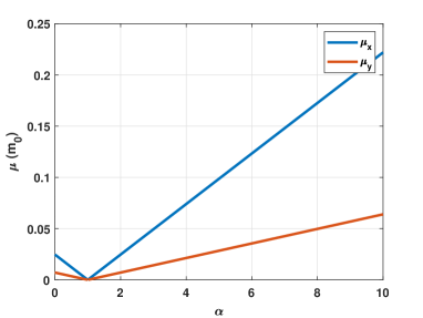
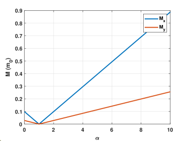
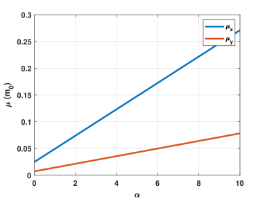
a) b) c) d)

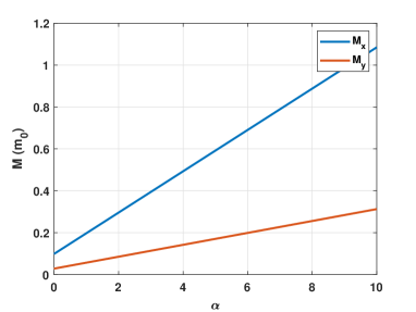
The relationship between the reduced masses and center-of-mass masses for other excitons depends on both the chosen spin and valley. We will also see the out-of-plane electric field, $\alpha$ can be used to tune the exciton binding energies, by tuning the effective mass parameters Katsnelson ; first . Specifically, for the three types of excitons, we see different behavior. For Type A excitons, we observe that both the reduced mass and that for the center-of-mass decrease linearly from $0\leq\alpha\leq 1.0$ with an increase of $\alpha$, while for $\alpha\geq 1$, the reduced mass and that for the center-of-mass increase linearly with an increase of $\alpha$. For Type B excitons, the reduced mass and that for the center-of-mass increase linearly for all $\alpha$, with increase of $\alpha$. Notably, for both Type A and Type B excitons, the reduced mass in x ($\mu_{x}$) and center-of-mass in X (M_X), are larger than the reduced mass in y ($\mu_{y}$) and center-of-mass in Y (M_Y).

(

(

Figure 3: (Color online) The dependence on $\alpha$ for Type C excitons (a) reduced exciton mass and (b) center-of-mass exciton mass. We employed the definition of the effective mass definitions of Eqn.(7) in the generation of these figures.

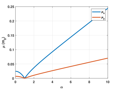
a) b)

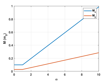
For Type C excitons we observe similar behaviour, seen above in Fig. 2. The reduced mass decreases non-linearly from $0\leq\alpha\leq 1$ and increases non-linearly for $\alpha\geq 1$. The center-of-mass mass is constant for $0\leq\alpha\leq 1$ and increases linearly for $\alpha\geq 1$, with increasing $\alpha$. Based on these results we can conclude that using a large value of $\alpha$ is beneficial for our binding energies, since it leads to larger values of binding energies, thus increasing the stability of the excitons.

II.3 Binding Energy of excitons with $h$-BN dielectric

The binding energy corresponding to the energy spectrum of an electron and hole described by Eq. (22), is given by

$$B=-\mathcal{E}_{00}=V_{0}-\hbar\sqrt{\frac{\gamma}{2\mu_{x}}}-\hbar\sqrt{\frac{\gamma}{2\mu_{y}}}=V_{0}-\hbar\sqrt{\frac{\gamma}{2\mu_{0}}}$$ (28)

In Eq.  (28), we define the quantity $\mu_{0}=\frac{\mu_{x}\mu_{y}}{(\sqrt{\mu_{x}}+\sqrt{\mu_{y}})^{2}}$ for convenience. In Fig. 3, we note that the binding energy of Type A excitons is decreased for increasing $D$ with chosen $\alpha$, and is increased for increasing $\alpha$, for chosen $D$. In our structure, we have thin sheets of h-BN dielectric between layers and occupy the the interlayer region of separation $D$. The dielectric is inserted to reduce degradation of the heterostructure and reduce the photoluminescence linewidth (PL) hBN . Each layer of h-BN is 0.33 nm thick and as such for experimental considerations, we restrict the number of layers to ten, or fewer, so as to be experimentally viable, while also forming a bound state of the exciton. Consequently, a desirable choice of parameters for the system includes a large binding energy, comparable in magnitude to prior results SuperfluidDipolar , and a low interlayer separation $D$ about 3.3 nm. We find that for larger values of $\alpha$, we can obtain larger binding energy for $D=20.0$ nm which corresponds to a value of $\alpha=6.0$. For all of Type A, B, C excitons, the choice of $\alpha=6.0$ or higher, allows for larger binding energy with a desirably low interlayer separation. We see that the larger the reduced mass, the greater the binding energy, as per our theoretical predictions. Too large an interlayer separation is not desirable since that would require a very large number of layers of h-BN dielectric.

For each type of our excitons (Type A, B, C), we find that a larger value of $\alpha$ satisfies the criteria for a small interlayer separation $D$, with a growing value of the binding energy, which is preferable for stability of the exciton. This behavior is illustrated in Figs. 3 through 5. When $\alpha=35.0$, we find that the binding energy of Type A, B and C excitons is 33.9 meV, 35.5 meV and 34.7 meV, respectively, for an interlayer separation of $D=3.3$ nm, which corresponds to $N_{L}=10$ layers of $h$-BN. It is worth noting that the corresponding value of $D_{0}$ for Type A, B and C excitons is 0.63 nm, 0.59 nm, and 0.62 nm, respectively. Consequently, the first-order Taylor series expansion is valid for the Coulomb potential. These results are as expected based on prior results Reichman .

(

(

Figure 4: The binding energy of Type A excitons as functions of the interlayer separation D, at different values of $\alpha$ - (a) $\alpha=6.0$, and (b) $\alpha=35.0$. We employed the binding energy definition of Eqn.(28), along with the effective mass definitions of Eqn. (11)-(15), in the generation of these figures.

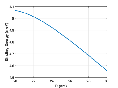
a) b)

(

(

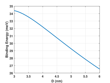
Figure 5: The binding energy for Type B excitons as functions of the interlayer separation $D$, at different values of $\alpha$ - (a) $\alpha=6.0$, and (b) $\alpha=35.0$. We employed the binding energy definition of Eqn.(28), along with the effective mass definitions of Eqn.(7), in the generation of these figures.

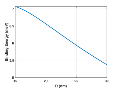
a) b)

(

(

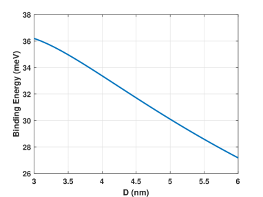
Figure 6: The binding energy of Type C excitons as functions of the interlayer separation $D$, at different values of $\alpha$ - (a) $\alpha=6.0$, and (b) $\alpha=35.0$. We employed the binding energy definition of Eqn.(28), along with the effective mass definitions of Eqn.(7), in the generation of these figures.

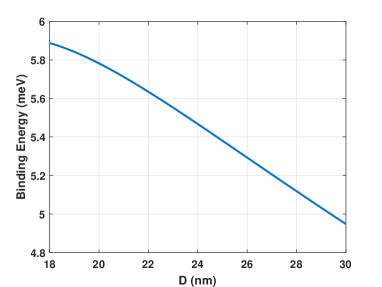
a) b)

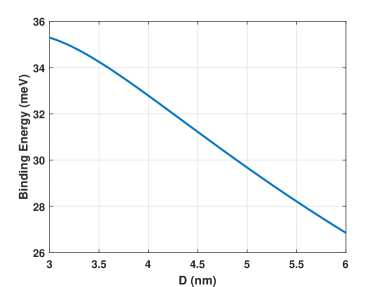
III Floquet engineering of tilted and gapped Dirac band structure

III.1 Circularly-polarized dressing field

It has been suggested that applying an external high-frequency optical dressing field of variable intensity, within the off-resonance regime, can modify the band structure, anisotropy, and band gaps of 1T^′-MoS₂ Floquet . Additionally, it was demonstrated that the electron-photon dressed states vary strongly with the polarization of the applied irradiation and reflect a full complexity of the low-energy Hamiltonian for non-irradiated material. Employing the numerical results for the dressed states obtained by using circularly-polarized irradiation, derived in  Ref. Floquet , we calculate the effective masses of the electron and hole using the following dispersion of irradiated subbands given by Eq. (29), with the hope of leveraging the frequency and intensity variables that allow for higher binding energies, and parameterise the superfluidity Floquet .

$$\varepsilon_{\tau=\pm 1}(\textbf{k}|\xi,s)=-\hbar\xi\upsilon_{-}k_{y}\pm\hbar\sqrt{\tilde{\Delta}^{2}_{\xi|s}(\lambda_{0})+[(\xi-sr_{E})\Delta_{0}+\upsilon_{2}k_{y}]^{2}+(\upsilon_{+}k_{y})^{2}+(\upsilon_{1}k_{x})^{2}}$$ (29)

where the additional irradiation-induced band gap $\tilde{\Delta}_{\xi|s}(\lambda_{0})$ takes the explicit form

$$\tilde{\Delta}_{\xi|s}(\lambda_{0})=\pm\sqrt{2c_{0}^{2}\upsilon_{1}\upsilon_{+}\Delta_{0}(1-sr_{E}\xi)+c_{0}^{4}\upsilon_{1}^{2}(\upsilon_{2}^{2}+\upsilon_{+}^{2})}$$ (30)

and, $\lambda_{0}=v_{F}eE_{0}/(\hbar\omega^{2})\ll 1$, $\upsilon_{-}$, $\upsilon_{+}$, $\upsilon_{1}$ and $\upsilon_{2}$ are as defined above as the Fermi velocities and the velocity correction terms. Furthermore, $\tau=\pm 1$ labels the electron/hole states related to the conduction and the valence bands, while $s=\pm 1$ is the real spin index. The spin-orbit coupling gap is $\Delta_{0}=0.81E^{(0)}$, $r_{E}=r=E_{z}/E_{c}$ is the relative value for the out-of-plane electric field, and $E_{c}$ stands for a critical field at which the band gap in 1T’-MoS₂ will be closed. It is important to notice that the energy dispersions are spin and valley polarized, i.e depend directly on indices $s$ and $\xi$. It is worth noting that the dressed states formed using linearly polarized dressing field are not studied in this paper. The model Hamiltonian within the effective mass approximation for a single electron-hole pair in a $\mathrm{1T^{\prime}-MoS_{2}}$ double layer is given by

$$\hat{H}_{0}=-\frac{\hbar^{2}}{2m_{x}^{e}}\frac{\partial^{2}}{\partial x_{1}^{2}}-\frac{\hbar^{2}}{2m_{y}^{e}}\left[\frac{\partial}{\partial y_{1}}-p_{e}^{(0)}\right]^{2}-\frac{\hbar^{2}}{2m_{x}^{h}}\frac{\partial^{2}}{\partial x_{2}^{2}}-\frac{\hbar^{2}}{2m_{y}^{h}}\left[\frac{\partial}{\partial y_{2}}-p_{h}^{(0)}\right]^{2}+V\left(\sqrt{r^{2}+D^{2}}\right)\ ,$$ (31)

where $V\left(\sqrt{r^{2}+D^{2}}\right)$ is the potential energy for electron-hole pair attraction, when the electron and hole are located in two different 2D planes. In Eq. (31), $m_{x}^{e}$, $m_{y}^{e}$, $m_{x}^{h}$, $m_{y}^{h}$, $p_{e}^{(0)}$, and $p_{h}^{(0)}$ are the constants, which can be obtained from Eq. (29) using the long wavelength expansion.

$$E(k)=E_{0}+\frac{\hbar^{2}}{2m^{*}_{x}}(k_{x}-k_{0,x})^{2}+\frac{\hbar^{2}}{2m^{*}_{y}}(k_{y}-k_{0,y})^{2}$$ (32)

Using the long wavelength expansion we are able to infer the following quantities

$$m_{x}^{e/h}=\dfrac{\sqrt{\Delta_{0}^{2}(\xi-rs)^{2}+\tilde{\Delta}^{2}_{\xi|s}(\lambda_{0})}}{\upsilon_{1}^{2}},\hskip 17.07182ptm_{y}^{e/h}=\frac{[\Delta_{0}^{2}(\xi-rs)^{2}+\tilde{\Delta}^{2}_{\xi|s}(\lambda_{0})]^{3/2}}{\Delta_{0}^{2}\upsilon_{+}^{2}(\xi-rs)^{2}+\tilde{\Delta}^{2}_{\xi|s}(\lambda_{0})(\upsilon_{2}^{2}+\upsilon_{+}^{2})}$$ (33)

$$\tilde{p}_{e/h}^{(0)}=\mp\frac{\left(\Delta_{0}^{2}(\xi-rs)^{2}+\tilde{\Delta}^{2}_{\xi|s}(\lambda_{0})\right)\cdot\left({rs\upsilon_{2}\Delta_{0}-\upsilon\Delta_{0}\xi+\upsilon_{-}\xi}\right)}{\upsilon_{+}^{2}\Delta_{0}^{2}(\xi-rs)^{2}+(\upsilon_{2}^{2}+\upsilon_{+}^{2})\tilde{\Delta}^{2}_{\xi|s}(\lambda_{0})}$$ (34)

The solutions to the center-of-mass and relative motion of the electron-hole pair are identical to those described in Section I.B, with the constants being the only difference.

III.2 Binding energy

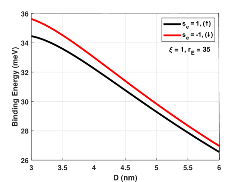
Figure 7: (Color online) The binding energies of excitons as functions of interlayer separation D for spin up (black) and spin down (red) electron-hole pairs. These results are for intravalley excitons at $\xi=1$. The following combination of parameters is used for each of the binding energy calculations - $\mathcal{I}_{df}=10^{9}$, $\omega=10^{16}$ Hz, $r_{E}=35$. We employed the binding energy definition of Eqn. (28), along with the effective mass definitions of Eqn.(33), in the generation of these figures.

In this section, we compute the binding energies of the excitons for chosen parameters. For our calculations, we confine our attention to $\xi=1.0$. We perform calculations for both combinations of spins, spin up ($s_{e}=+1$) electrons and spin down holes, and spin down electrons ($s_{e}=-1$) and spin up holes. In our calculations, it is worth noting that the mass of the holes is effectively that of an electron of opposite spin. In Fig. 6, the irradiation intensity $\mathcal{I}_{df}=10^{9}$, the frequency of irradiation $\omega=10^{16}$ Hz, and the relative value of the out-of-plane electric field $r_{E}=35.0$. Our calculations show that spin down electrons-spin up hole pairs have a higher binding energy than spin up electrons-spin down hole pairs. These binding energies are also on a similar scale as the results outlined in Sec. I.D in particular Figs. 3(b), 4(b) and 5(b).

It is worth considering certain parameter restrictions and suggestions. This would enable us to obtain the binding energies for chosen interlayer eparation. Our choice of parameters leads to a higher binding energy for smaller interlayer separation. We find that choosing a $r_{E}$ of larger magnitude, leads to this effect. Additionally, the value of the gap must be real and positive.

Furthermore, it is worth noting that changing $\omega$ and $\mathcal{I}_{df}$ does not induce an appreciable change in the effective masses. In accordance with prior results Floquet , we find that the larger band gaps tend to be reduced by circularly polarized dressing field. The orientation and anisotropy for the constant-energy cut dispersions in 1T’-MoS₂ remains unchanged under circularly-polarized irradiation. The additional energy gap induced by the irradiation is contributed by the $\tilde{\Delta}$ term in Eq. (30).

IV Collective excitations for spatially separated electrons and holes

In this section, we examine the dilute limit for gases of electrons and holes in a double layer of 1T^′-MoS₂. In this limit, we consider dipolar Type A and Type B excitons. However, the analysis holds true for all other combinations of types of excitons, i.e., Type A and Type C, and Type B and Type C. Henceforth, we will refer to Type A, B and C excitons, simply as $A$, $B$ and $C$ excitons for brevity. In this section we formulate the sound velocity, which will determine whether the Landau criterion for superfluidity is satisfied.

We expect that at $T=0$ K almost all $A$ and $B$ excitons condense into a BEC of $A$ and $B$ excitons. This allows us to assume the formation of a binary mixture of BECs. We will describe this two-component weakly interacting Bose gas of excitons following the procedure, described in Refs. SuperfluidDipolar ; HighTempSuperOleg . We then examine this mixture within the Bogoliubov approximation Abrikosov . Only the interactions between the condensate and noncondensate particles are considered, since we assume almost all the particles belong to the BEC. The interactions between noncondensate particles are neglected. This allows us to diagnolize the many particle Hamiltonian. This reduces the product of four operators in the interaction term of the Hamiltonian by replacing it with a pair consisting of a product of two operators LifPit . The condensate operators are replaced by numbers, and the resulting Hamiltonian is quadratic with respect to the creation and annihilation operators. Employing the Bogoliubov approximation LifPit , generalized for a two-component weakly interacting Bose gas, we obtain the chemical potential $\mu$ of the excitonic system by minimizing $\hat{H}_{0}-\mu\hat{N}$ with respect to the 2D concentration $n$ minimizeHmuN , where $\hat{N}$ denotes the number operator

$$\hat{N}=\sum_{\textbf{P}}a^{{\dagger}}_{\textbf{p}A}a_{\textbf{p}A}+\sum_{\textbf{P}}a^{{\dagger}}_{\textbf{p}B}a_{\textbf{p}B}$$ (35)

and $H_{0}$ is the Hamiltonian describing the particles in the condensate with zero momentum $\textbf{p}=0$. In the Bogoliubov approximation, we assume $N=N_{0}$, $a^{{\dagger}}_{\textbf{p}=0,A(B)}=\sqrt{N_{0A(B)}}e^{-i\Theta_{A(B)}}$, and $a_{\textbf{p}=0,A(B)}=\sqrt{N_{0A(B)}}e^{i\Theta_{A(B)}}$, where $N$ is the total number of all excitons in the condensate, $N_{0A(B)}$ and $\Theta_{A(B)}$ are the number and phase for $A(B)$ excitons in the condensate. In the small momentum limit, $p=\hbar k$ when $\varepsilon_{(0)A}(P,\Theta)\ll G_{AA}$, and $\varepsilon_{(0)B}(P,\Theta)\ll G_{BB}$ we expand the spectrum of collective excitations $\varepsilon_{j}(p,\Theta)$ up to first order with respect to the momentum $p$ and obtain two sound modes of the collective excitations $\varepsilon_{j}(p,\Theta)=c_{j}(\Theta)p$, where $c_{j}(\Theta)$ is the sound velocity given by

$$c_{j}(\Theta)=\sqrt{\frac{G_{AA}}{2M_{0A}(\Theta)}+\frac{G_{BB}}{2M_{0B}(\Theta)}+(-1)^{j-1}\sqrt{\left(\frac{G_{AA}}{2M_{0A}(\Theta)}-\frac{G_{BB}}{2M_{0B}(\Theta)}\right)^{2}+\frac{G^{2}_{AB}}{M_{A}(\Theta)M_{B}(\Theta)}}}$$ (36)

In the limit of large momenta when $\varepsilon_{(0)A}(P,\Theta)\gg G_{AA}$, and $\varepsilon_{(0)B}(P,\Theta)\gg G_{BB}$, we get two parabolic modes of collective excitations with the spectra $\varepsilon_{1}(p,\Theta)=\varepsilon_{(0)A}(p,\Theta)$ and $\varepsilon_{2}(p,\Theta)=\varepsilon_{(0)B}(p,\Theta)$. The Hamiltonian $\hat{H}_{\text{col}}$ of collective excitations, corresponding to two branches of the spectrum, in the Bogoliubov approximation for the entire two-component anisotropic system is given by

$$\hat{H}_{\text{col}}=\sum_{\textbf{P}\neq 0}\varepsilon_{1}(P,\Theta)\alpha^{{\dagger}}_{1\textbf{p}}\alpha_{1\textbf{p}}+\sum_{\textbf{P}\neq 0}\varepsilon_{2}(P,\Theta)\alpha^{{\dagger}}_{2\textbf{p}}\alpha_{2\textbf{p}}\ ,$$ (37)

where $\alpha^{{\dagger}}_{j\textbf{P}}$ and $\alpha_{j\textbf{P}}$ are the creation and annihilation Bose operators for the quasiparticles with the energy dispersion corresponding to the $j$th mode of the spectrum of the collective excitations. For simplicity, we consider the specific case when the densities of $A$ and $B$ excitons are the same as $n_{A}=n_{B}=n/2$. Following the standard procedure for calculations outlined in the Supplemental Materials, Section II in SuppMat we obtain the spectrum of collective excitations

$$\varepsilon_{j}(P,\Theta)=\sqrt{\frac{\omega^{2}_{A}(P,\Theta)+\omega^{2}_{B}(P,\Theta)+(-1)^{j-1}\sqrt{\left[\omega^{2}_{A}(P,\Theta)-\omega^{2}_{B}(P,\Theta)\right]^{2}+4g^{2}n^{2}\varepsilon_{(0)A}(P,\Theta)\varepsilon_{(0)B}(P,\Theta)}}{2}}$$ (38)

and the sound velocity at $n_{A}=n_{B}=n/2$ is obtained as

$$c_{j}(\Theta)=\sqrt{\frac{gn}{2}\left(\frac{1}{2M_{0A}(\Theta)}+\frac{1}{2M_{0B}(\Theta)}+(-1)^{j-1}\sqrt{\left(\frac{1}{2M_{0A}(\Theta)}-\frac{1}{2M_{0B}(\Theta)}\right)^{2}+\frac{1}{M_{0A}(\Theta)M_{0B}(\Theta)}}\right)}$$ (39)

It follows from Eq. (39) that there is only one nonzero sound velocity at $n_{A}=n_{B}=n/2$ given by

$$c_{S}(\Theta)=\sqrt{\frac{gn}{2}\left(\frac{1}{M_{0A}(\Theta)}+\frac{1}{M_{0B}(\Theta)}\right)}$$ (40)

It is also worth noting that the large interlayer separation $D$, between the double layer allows us to neglect the exchange interactions in the electron-hole system. This is caused by a low tunneling probability , caused by the shielding of the dipole-dipole interaction by the dielectric (h-BN) that separates the layers in the double layer HighTempSuperOleg .

V Superfluidity

In this section, we determine the criterion for which a weakly interacting Bose gas of dipolar excitons can form a superfluid. Since at low momenta the energy spectrum of quasiparticles of a weakly interacting gas of excitons is soundlike, this system satisfies the Landau criterion for superfluidity LifPit . The critical velocity for superfluidity is given by $v_{c}=\text{min}(c_{1}(\Theta),c_{2}(\Theta))$ since the quasiparticles are created at velocities exceeding that of sound for the lowest mode of the quasiparticle dispersion. Additionally, it is angular dependent. The density of the superfluid $\rho_{s}(T)$ is defined as $\rho_{s}(T)=\rho-\rho_{n}(T)$, where $\rho=M_{A}n_{A}+M_{B}n_{B}$, is the total 2D density of the system and $\rho_{n}(T)$ is the density of the normal component. We define the normal component $\rho_{n}(T)$ in the usual way nanomatGabriel . Assume that the excitonic system moves with velocity u, which means that the superfluid component has velocity u. At finite temperatures $T$, dissipating quasiparticles will emerge in this system. Since their density is small at low temperatures, one may assume that the gas of quasiparticles is an ideal Bose gas. We will obtain the density of the superfluid component in the anisotropic system following the procedure, described in Ref. phosphoreneOGR . To calculate the superfluid component density, we begin by defining the mass current J for a Bose gas for quasiparticles in the frame of reference where the superfluid component is at rest by

$$\textbf{J}=s\int\frac{d^{2}P}{(2\pi\hbar)^{2}}\textbf{P}\left[f[\varepsilon_{1}(P,\Theta)-\textbf{P}\textbf{u}]+f[\varepsilon_{2}(P,\Theta)-\textbf{P}\cdot\textbf{u}]\right]$$ (41)

where $f[\varepsilon_{1}(P,\Theta)]=\{\text{exp}[\varepsilon_{1}(P,\Theta)/(k_{B}T)]-1\}^{-1}$ and $f[\varepsilon_{2}(P,\Theta)]=\{\text{exp}[\varepsilon_{2}(P,\Theta)/(k_{B}T)]-1\}^{-1}$ are the Bose-Einstein distribution functions for the quasiparticles with the angle dependent dispersions $\varepsilon_{1}(P,\Theta)$ and $\varepsilon_{2}(P,\Theta)$ respectively, $s$ is the spin degeneracy factor, and $k_{B}$ is the Boltzmann constant. Expanding the expression under the integral in terms of $\textbf{P}\textbf{u}/k_{B}T$ and restricting ourselves to the first-order term, we obtain

$$\textbf{J}=-\frac{s}{k_{B}T}\int\frac{d^{2}P}{(2\pi\hbar)^{2}}\textbf{P}(\textbf{P}\cdot\textbf{u})\left(\frac{\partial f[\varepsilon_{1}(P,\Theta)]}{\partial\varepsilon_{1}(P,\Theta)}+\frac{\partial f[\varepsilon_{2}(P,\Theta)]}{\partial\varepsilon_{2}(P,\Theta)}\right)$$ (42)

The normal density $\rho_{n}$ in the anisotropic system takes tensor form. We define the tensor elements for the normal component density $\rho^{(ij)}_{n}(T)$ by

$$J_{i}=\rho^{(ij)}_{n}(T)u_{j}$$ (43)

where $i,j$ denote either $x,y$ component. Assuming that the vector u is parallel to the $OX$ axis and has the same direction as this axis, we have $\textbf{u}=u_{x}\textbf{i}$ and $\textbf{P}=P_{x}\textbf{i}+P_{y}\textbf{j}$ and $\textbf{P}\cdot\textbf{u}=P_{x}u_{x}$, $\textbf{P}(\textbf{P}\cdot\textbf{u})=P_{x}^{2}u_{x}\textbf{i}+P_{x}P_{y}u_{x}\textbf{j}$, where i and j are unit vectors in the $x$ and $y$ directions, respectively. We then obtain

$$J_{x}=-\frac{s}{k_{B}T}\int_{0}^{\infty}dP\frac{P^{3}}{(2\pi\hbar)^{2}}\int_{0}^{2\pi}d\Theta\left(\frac{\partial f[\varepsilon_{1}(P,\Theta)]}{\partial\varepsilon_{1}(P,\Theta)}+\frac{\partial f[\varepsilon_{2}(P,\Theta)]}{\partial\varepsilon_{2}(P,\Theta)}\right)\cos^{2}\Theta\ u_{x}$$ (44)

Using the definition of the density for the normal component from Eq. (43), we obtain

$$\rho^{(xx)}_{n}(T)=\frac{s}{k_{B}T}\int_{0}^{\infty}dP\frac{P^{3}}{(2\pi\hbar)^{2}}\int_{0}^{2\pi}d\Theta\left(\frac{\text{exp}[\varepsilon_{1}(P,\Theta)/(k_{B}T)]}{\{[\text{exp}[\varepsilon_{1}(P,\Theta)/(k_{B}T)]-1\}^{2}}+\frac{\text{exp}[\varepsilon_{2}(P,\Theta)/(k_{B}T)]}{\{[\text{exp}[\varepsilon_{2}(P,\Theta)/(k_{B}T)]-1\}^{2}}\right)\cos^{2}\Theta$$ (45)

Furthermore, from Eq. (42), we can also obtain

$$J_{y} =-\frac{s}{k_{B}T}\int_{0}^{\infty}\frac{d^{2}P}{(2\pi\hbar)^{2}}P_{x}P_{y}\left(\frac{\partial f[\varepsilon_{1}(P,\Theta)]}{\partial\varepsilon_{1}(P,\Theta)}+\frac{\partial f[\varepsilon_{2}(P,\Theta)]}{\partial\varepsilon_{2}(P,\Theta)}\right)u_{x}$$ (46)

$$=\frac{s}{k_{B}T}\int_{0}^{\infty}dP\frac{P^{3}}{(2\pi\hbar)^{2}}\int_{0}^{2\pi}d\Theta\left(\frac{\text{exp}[\varepsilon_{1}(P,\Theta)/(k_{B}T)]}{\{[\text{exp}[\varepsilon_{1}(P,\Theta)/(k_{B}T)]-1\}^{2}}+\frac{\text{exp}[\varepsilon_{2}(P,\Theta)/(k_{B}T)]}{\{[\text{exp}[\varepsilon_{2}(P,\Theta)/(k_{B}T)]-1\}^{2}}\right)\cos\Theta\sin\Theta\ u_{x}$$ (47)

The integral in Eq. (47) is zero, since the $\Theta$ integral over the period of the integrand vanishes. Therefore, one determines that $\rho^{(xy)}_{n}=0$. Now, assuming that the vector u is parallel to the $OY$ axis, we obtain analogously the following relations:

$$\rho^{(yy)}_{n}(T) =\frac{s}{k_{B}T}\int_{0}^{\infty}dP\frac{P^{3}}{(2\pi\hbar)^{2}}\int_{0}^{2\pi}d\Theta\left(\frac{\text{exp}[\varepsilon_{1}(P,\Theta)/(k_{B}T)]}{\{[\text{exp}[\varepsilon_{1}(P,\Theta)/(k_{B}T)]-1\}^{2}}+\frac{\text{exp}[\varepsilon_{2}(P,\Theta)/(k_{B}T)]}{\{[\text{exp}[\varepsilon_{2}(P,\Theta)/(k_{B}T)]-1\}^{2}}\right)\sin^{2}\Theta$$ (48)

$$\rho^{(yx)}(T) =0$$ (49)

By defining the tensor of the concentration of the normal component as the linear response of the flow of quasiparticles on the external velocity as $n^{(ij)}_{n}=\rho^{(ij)}_{n}/M_{i}$, one obtains

$$n^{(xx)}_{n}(T) =\frac{s}{k_{B}M_{x}T}\int_{0}^{\infty}dP\frac{P^{3}}{(2\pi\hbar)^{2}}\int_{0}^{2\pi}d\Theta\left(\frac{\text{exp}[\varepsilon_{1}(P,\Theta)/(k_{B}T)]}{\{[\text{exp}[\varepsilon_{1}(P,\Theta)/(k_{B}T)]-1\}^{2}}+\frac{\text{exp}[\varepsilon_{2}(P,\Theta)/(k_{B}T)]}{\{[\text{exp}[\varepsilon_{2}(P,\Theta)/(k_{B}T)]-1\}^{2}}\right)\cos^{2}\Theta$$ (50)

$$n^{(yy)}_{n}(T) =\frac{s}{k_{B}M_{y}T}\int_{0}^{\infty}dP\frac{P^{3}}{(2\pi\hbar)^{2}}\int_{0}^{2\pi}d\Theta\left(\frac{\text{exp}[\varepsilon_{1}(P,\Theta)/(k_{B}T)]}{\{[\text{exp}[\varepsilon_{1}(P,\Theta)/(k_{B}T)]-1\}^{2}}+\frac{\text{exp}[\varepsilon_{2}(P,\Theta)/(k_{B}T)]}{\{[\text{exp}[\varepsilon_{2}(P,\Theta)/(k_{B}T)]-1\}^{2}}\right)\sin^{2}\Theta$$ (51)

$$n^{(xy)}(T)=0,\hskip 5.69046ptn^{(yx)}(T)=0$$ (52)

The linear response of the flow of quasiparticles $\textbf{J}_{qp}$ with respect to the external velocity at any angle measured from the $OX$ direction is given in terms of the angle-dependent concentration for the normal component $\tilde{n}_{n}(\Theta,T)$ as

$$|\textbf{J}_{{qp}}| = |n^{(xx)}_{n}(T)\ u_{x}\ \textbf{i}+n^{(yy)}_{n}(T)\ u_{y}\ \textbf{j}|$$ (53)

$$= \sqrt{[n^{(xx)}_{n}(T)]^{2}u^{2}\cos^{2}\Theta+[n^{(yy)}_{n}(T)]^{2}u^{2}\sin^{2}\Theta}=\tilde{n}(\Theta,T)u\ ,$$

where the concentration of the normal component is

$$\tilde{n}_{n}(\Theta,T)=\sqrt{[n^{xx}_{n}(T)]^{2}\cos^{2}\Theta+[n^{yy}_{n}(T)]^{2}\sin^{2}\Theta}\ .$$ (54)

From Eq. (54) it follows that $n^{(xx)}_{n}=\tilde{n}_{n}(\Theta=0)$ and $n^{(yy)}_{n}=\tilde{n}_{n}(\Theta=\pi/2)$. We can then rewrite Eq. (54) in the following form:

$$\tilde{n}_{n}(\Theta,T)=\sqrt{\frac{[n^{xx}_{n}(T)]^{2}+[n^{yy}_{n}(T)]^{2}}{2}+\frac{([n^{xx}_{n}(T)]^{2}-[n^{yy}_{n}(T)]^{2})\cos(2\Theta)}{2}}$$ (55)

We define the angle-dependent concentration of the superfluid component $\tilde{n}_{s}(\Theta,T)$ by

$$\tilde{n}_{s}(\Theta,T)=n-\tilde{n}_{n}(\Theta,T)\ ,$$ (56)

where $n$ is the total concentration of the excitons. The mean-field critical temperature $T_{c}(\Theta)$ of the phase transition related to the occurrence of superfluidity in the direction with the angle $\Theta$ relative to the $x$ direction is determined by the condition $\tilde{n}_{n}(\Theta,T)=n$.

V.1 Superfluidity for the soundlike spectrum of collective excitations

In a straightforward way, it follows from Eq. (36) that for $j=2$ the sound velocity vanishes. Therefore, we only take into account the spectrum of collective excitations for $j=1$. According to Ref. LandauStat , it is clear that we need a finite sound velocity for superfluidity. Since the branch of collective excitations at zero sound velocity corresponds to zero energy of the quasiparticles (which means that no quasiparticles are created at zero sound velocity), this branch does not lead to dissipation of energy, thereby resulting in finite velocity and does not affect the Landau critical velocity. The weakly interacting gas of dipolar excitons, satisifies the Landau criterion for superfluidity since for small momenta, the energy spectrum of the quasiparticles in the weakly interacting gas of dipolar excitons at $j=1$ is soundlike with sound velocity

$$c_{1}(\Theta)=\sqrt{\frac{gn_{A}}{M_{OA}(\Theta)}+\frac{gn_{B}}{M_{OB}(\Theta)}}\ .$$ (57)

Clearly the ideal Bose gas has no branch with non-zero sound velocity, thus not demonstrating superfluidity. At low temperatures, the two-component system of dipolar excitons exhibits superfluidity due to exciton-exciton interactions. With this new knowledge, we can again return to our definition for the mass current in Eq. (42) rewritten as

$$\textbf{J}={s}\int\frac{d^{2}P}{(2\pi\hbar)^{2}}\textbf{P}f[\varepsilon_{1}(P,\Theta)-\textbf{P}\cdot\textbf{u}]\ ,$$ (58)

where $s=16$ is the spin degeneracy factor, $f[\varepsilon_{1}(p)]$ is the Bose-Einstein distribution function for the quasiparticles with dispersion $\varepsilon_{1}(p)$ and $k_{B}$ is the Boltzmann constant. Expanding this to first order with respect to $\textbf{P}\cdot\textbf{u}/(k_{B}T)$, we obtain

$$\textbf{J}=-s\frac{\textbf{u}}{2}\int\frac{d^{2}P}{(2\pi\hbar)^{2}}P^{2}\frac{\partial f[\varepsilon_{1}(P,\Theta)]}{\partial\varepsilon_{1}(P,\Theta)}\ .$$ (59)

The density of the normal component $\rho_{n}$, in the moving weakly-interacting Bose gas of dipolar excitons is defined as $\textbf{J}=\rho_{n}\textbf{u}\ .$ Therefore,

$$\rho_{n}=-\frac{s}{2}\int\frac{d^{2}P}{(2\pi\hbar)^{2}}P^{2}\frac{\partial f[\varepsilon_{1}(P,\Theta)]}{\partial\varepsilon_{1}(P,\Theta)}$$ (60)

By substituting the sound velocity $\varepsilon_{1}(P,\Theta)=c_{1}(\Theta)P$ into Eq. (60), we obtain

$$\rho_{n}(T)=\frac{3s\zeta(3)}{2\pi\hbar^{2}c_{1}^{4}(\Theta)}k_{B}^{3}T^{3}$$ (61)

The mean field critical temperature $T_{c}$ of the phase transition at which the superfluidity occurs, implying neglecting the interaction between the quasiparticles, is obtain from the condition $\rho_{s}(T_{c})=0$:

$$\rho_{n}(T_{c},\Theta)=\rho=M_{OA}n_{A}+M_{OB}n_{B}$$ (62)

At low temperatures $k_{B}T\ll M_{A(B)}c_{1}(\Theta)^{2}$, by substituting Eqn. (62) into Eqn. (61) one derives

$$T_{c}(\Theta)=\left[\frac{2\pi\hbar^{2}\rho c_{1}^{4}(\Theta)}{3\zeta(3)sk_{B}^{3}}\right]^{1/3}\ .$$ (63)

In this paper, we have obtained the mean-field critical temperature $T_{c}$ of the phase transition at which superfluidity appears without claiming BEC in a 2D system at finite temperature.

VI Results and Discussion

VI.1 Computation of sound velocity as function of different parameters

We now demonstrate numerically the dependence of the sound velocity and the critical temperature on the angle $\Theta$ and the chose parameters for an experiment such as the interlayer separation $D$ and the relative value of the out-of-plane electric field $\alpha$. It is worth noting that the formalism outlined above can apply to any pairs of excitons - A and B, A and C, and B and C exciton pairs. For the masses in this section, we will be looking at the non-Floquet engineered masses specified via Eqn. (7).

In Fig. (8), the sound velocity $c_{1}$ is plotted as a function of the angle $\Theta$. The sound velocity is seen to have a maximum at $\pi/2$ and $3\pi/2$ and is minimum at $\pi$ and $2\pi$. The sound velocity oscillates for all pairs of excitons and has maxima at around $1.5\times 10^{5}$ m/s for all pairs of excitons for the parameters we have chosen below. The minima are about $8.0\times 10^{4}$ m/s.

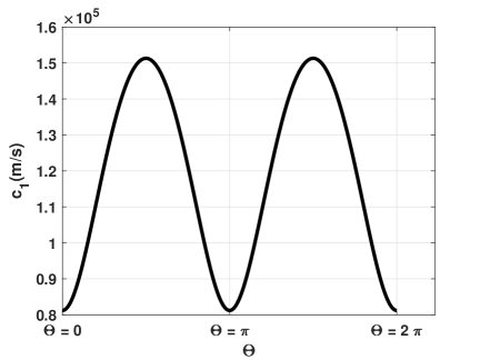
Figure 8: The dependence of the sound velocity $c_{1}$ as a function of $\Theta$ for the pairing of Type A and B excitons. The difference in the sound velocity for different pairings of excitons, as a function of $\Theta$ is negligibly small. The parameters that have been kept constant for this are $n=1$ x $10^{11}$cm^-2, $D=25$ nm and $\alpha=35$. We employed the definition of the sound velocity in Eqn. (40) in the generation of these figures.

In Fig. (9) below, we plot the dependence of the sound velocity $c_{1}$ as a function of the interlayer separation $D$ (nm). It is worth noting that higher values of interlayer separation lead to higher sound velocities for all pairs of excitons; It is worth noting that at our recommended number h-BN layers - 10 layers at 3.3 Å per layer for an interlayer separation of 3.3 nm - the sound velocity is around 2 x 10⁴ m/s.

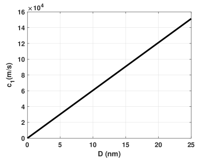
Figure 9: The dependence of the sound velocity $c_{1}$ as a function of $D$ for different pairings of excitons. The difference in the sound velocity for different pairings of excitons, as a function of $D$ is negligibly small. The parameters that have been kept constant for this are $n=1$ x $10^{11}$cm^-2, $\alpha=35$ and $\Theta=\pi/2$. We employed the definition of the sound velocity in Eqn. (40) in the generation of these figures.

In Fig. 10, we plot the sound velocity as a function of the relative value of the out-of-plane electric field $\alpha$. Here we notice some distinctly different behavior for the exciton-exciton pairs, specifically in the range $0<\alpha<1$. For A and B, and A and C exciton-exciton pairs, the sound velocity initially has a base value which increases from $0$ to $1.0$. When $\alpha=1.0$, there is no calculated sound velocity because at this critical value of $\alpha$, the A excitons have zero center-of-mass, as demonstrated in Fig. 1(b). The sound velocity is monotonically decreasing beyond $\alpha>1$. For the pairing of B and C excitons, the sound velocity decreases from $0<\alpha<1$, before steadily declining at larger values of $\alpha$. In Fig. 9 below this behaviour is not captured appreciably, and at about $\alpha>2$ the sound velocity plateaus off to a fairly constant value.

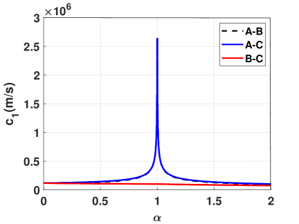
Figure 10: (Color online) The dependence of the sound velocity $c_{1}$ as a function of $\alpha$ for different pairings of excitons. The parameters that have been kept constant for this are $n=1$ x $10^{11}$cm^-2, $D=3.3$ nm and $\Theta=\pi/2$. We employed the definition of the sound velocity in Eqn. (40) in the generation of these figures.

VI.2 The critical temperature

We now turn our attention to calculating the critical temperature as functions of various chosen parameters. We begin by investigating the dependence of the critical temperature as a function of the angle $\Theta$ shown in Fig. (11). As expected, the behavior here is also oscillatory, displaying similar maxima and minima as the dependence of the sound velocity on the angle $\Theta$. The different pairs of excitons demonstrate negligibly different critical temperatures. When zoomed in the A and C exciton-exciton pairs display generally higher critical temperatures, and B and C exciton-exciton pairs display generally lower critical temperatures, but notably the difference is a very small percentage of their mean value.

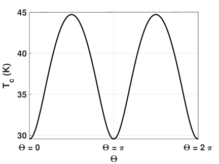
Figure 11: The dependence of the critical temperature as a function of $\Theta$ for different pairing of A and B excitons. The difference in the critical temperature for different pairings of excitons, as a function of $\Theta$ is negligibly small. The parameters that have been kept constant for this are $n=20$ x $10^{11}$cm^-2, $D=3.3$ nm and $\alpha=35$. We employed the definition of the critical temperature, $T_{c}$ in Eqn. (63) in the generation of these figures.

We plot the critical temperature as a function of the interlayer separation $D$. We chose the range $3.0\ \textnormal{nm}~{}\leq~{}D~{}\leq~{}6.0\ \textnormal{nm}$ since this is a range of interest for a feasible number of h-BN layers in an experiment. This smaller range also helps us see with greater resolution the contrast between the different pairings of exciton-exciton pairings. Larger interlayer separations lead to higher critical temperatures.

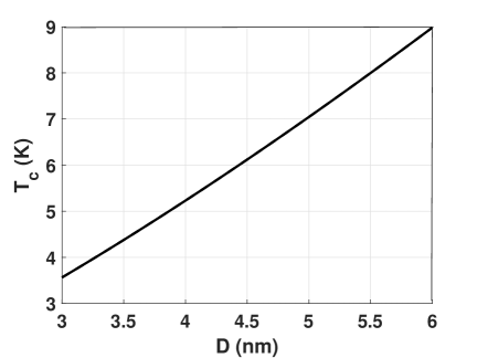
Figure 12: The dependence of the critical temperature as a function of $D$ for different pairings of excitons. The difference in the critical temperature for different pairings of excitons, as a function of $D$ is negligibly small. The parameters that have been kept constant for this are $n=1$ x $10^{11}$cm^-2, $\Theta=\pi/2$ and $\alpha=35$. We employed the definition of the critical temperature, $T_{c}$ in Eqn. (63) in the generation of these figures.

We then investigate the critical temperature as a function of $\alpha$. Our results are presented in Fig.  13. The critical temperature is increased in the range $0<\alpha<1.0$ for A-B and A-C exciton-exciton pairs. At $\alpha=1.0$, the critical temperature is notably unable to be calculated because of the zero center-of-mass for A excitons. For all pairs of excitons, the critical temperature is decreased beyond $\alpha>1.0$. Since using a large values of $\alpha$ is favorable for a larger binding energy, and thus stability and lifetime of the exciton, we need to balance the choice of the parameter with the diminishing of the critical temperature $T_{c}$.

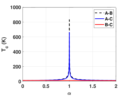
Figure 13: (Color online) The dependence of the critical temperature as a function of $\alpha$ for different pairings of excitons. The parameters that have been kept constant for this are $n=1$ x $10^{11}$cm^-2, $\Theta=\pi/2$ and $D=3.3$ nm. We employed the definition of the critical temperature, $T_{c}$ in Eqn. (63) in the generation of these figures.

It is worth calculating the critical temperature for the set of experimental parameters we recommend. These are as a function of the exciton concentration $n$, where $n=n_{A}/2=n_{B}/2$. For this calculation, we set the parameters as follows - $\alpha=35.0$, $D=3.3$ nm (corresponding to ten layers of h-BN) and $\Theta=\pi/2$. Our results are presented in Fig. 14. All combinations of exciton-exciton pairs lead to fairly similar critical temperatures for different concentrations of excitons. Zooming in, one can see that the A-C exciton-exciton pair has a higher critical temperature than the other two combinations, while B-C has a lower critical temperature, for a chosen set of parameters. Since we consider the dilute limit, we demand that the average distance between the excitons is much larger than the interlayer separation. Mathematically, this corresponds to $n\ll 1/(\pi D^{2})$.

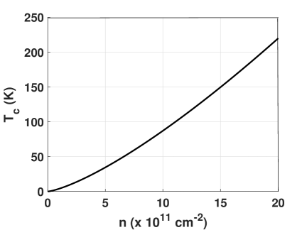
Figure 14: The dependence of the critical temperature as a function of $n$ for different pairings of excitons. The difference in the critical temperature for different pairings of excitons, as a function of $n$ is negligibly small. The parameters that have been kept constant for this are $\alpha=35$, $\Theta=\pi/2$ and $D=3.3$ nm. We employed the definition of the critical temperature, $T_{c}$ in Eqn. (63) in the generation of these figures.

It is not necessary to restrict our attention to the condition $n=n_{A}/2=n_{B}/2$, for any two pairs of excitons. As such, in Fig. 14, we investigate the dependence of $T_{c}$ as a function of the exciton densities. We notice that an increase in exciton density for both types of excitons leads to a higher critical temperature. We note that the increase in concentration to a value of $n_{A}=n_{B}=2.0\times 10^{12}$ cm^-2, leads to a critical temperature of around $T_{c}=250$ K, which holds true for any combination of any two excitons of A, B or C. It is worth noting that in the pairing of B and C excitons, the concentration of B excitons has a more pronounced effect on the $T_{c}$.

(

(

(

Figure 15: (Color online) The dependence of the critical temperature as a function of the exicton densities for different pairings of excitons. The parameters that have been kept constant for this are $\alpha=35$, $\Theta=\pi/2$ and $D=3.3$ nm. The colorbar on the side is the critical temperature $T_{c}$ in Kelvins. We employed the definition of the critical temperature, $T_{c}$ in Eqn. (63) in the generation of these figures.

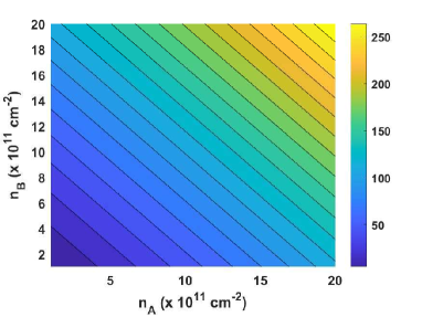
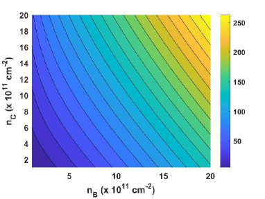
a) b) c)

VII Conclusions and discussion

In this paper, we have investigated the binding energies, wave functions, collective properties and superfluidity of dipolar excitons in a double layer of massive anisotropic tilted Dirac systems irradiated by circularly polarized light. For our calculations as an example we have considered a double layer of 1T^′-MoS₂. The binding energy of the three different types of excitons has been obtained by employing the harmonic oscillator approximation. It is found that using a large value of a perpendicular electric field $\alpha$ leads to a large binding energy at a small enough interlayer separation $D$ to use an experimentally reasonable number of layers of h-bN dielectric. It is also found that using Floquet engineering of the energy bands leads to no appreciable change in the effective mass of the electrons or holes. However, it is worth noting that it is unclear if using a larger $\lambda_{0}$ value, corresponding to a larger irradiation intensity to frequency ratio would lead to an appreciable increase in the effective mass. To study this, a second-order or higher expansion of the energy dispersion would be necessitated. However, as seen in Fig. 6, the binding energy of the excitons is very close in magnitude to the binding energy without any circularly polarized dressing field applied.

We note that for dipolar excitons in 1T^′-MoS₂, the spectrum of collective excitations is angular dependent. Furthermore, for dipolar excitons in double-layer 1T^′-MoS₂, the normal and superfluid concentrations have a tensor form whose components depend on the direction of exciton flow. Additionally, for the double-layer, the mean-field critical temperature of superfluidity depends on the direction of exciton flow as demonstrated in Fig. 10. Therefore, the influence of the anisotropy of the dispersion relation of dipolar excitons in a double layer of 1T^′-MoS₂ with tilted Dirac bands has been investigated. We conclude that the anisotropy of the energy band structure of the in 1T^′-MoS₂ exhibits superfluidity at low temperatures due to the dipole-dipole repulsion between the dipolar excitons. It is crucial to note that the binding energy of dipolar excitons and mean-field critical temperature for superfluidity are sensitive to the electron and hole effective masses. In terms of experimental observation, we can exploit some features of the photoluminescence spectrum, including emission traces caused by phonon-assisted recombination of momentum-space dark excitons. The microscopic theory for this was recently developed Malic . The theory can be applied specifically to the case of momentum-space dark excitons in a double layer of 1T^′-MoS₂. This warrants further development of the formalism in conjunction with analysis of experimental results of phonon-assisted photoluminiscence experiments. Experimental findings include the observation of intervalley momentum-forbidden excitons influenced by compressive strain, serving as an ultrasensitive optical strain sensing mechanism, and the repulsion-driven propagation of dark spin-forbidden excitons, allowing for the propagation of valley and spin information across TMD samples for diverse optoelectronic applications GrossPoster ; OpticalReadout ; StrainExciton . We hope that our analytical and numerical results will provide motivation for future experimental and theoretical investigations regarding the effects of circularly polarized light on excitonic BEC and superfluidity for double layer 1T^′-MoS₂.

Appendix A The Hamiltonian of the charge carriers in a monolayer of 1T^′-MoS₂

The low-energy $\mathbf{k}\cdot{\mathbf{p}}$ Hamiltonian is constructed based on the symmetry properties of the valence and conduction bands of the MoS₂ system. The Hamiltonian of the charge carriers in tilted a monolayer of 1T^′-MoS₂ is presented in Appendix A. The valence and conduction bands mainly consist of $d$-orbitals of Mo atoms and by $p_{y}$-orbitals of S atoms, respectively. $\lambda=\pm$ is used to distinguish the locations of two independent Dirac points. $\upsilon_{1}=3.87\times 10^{5}$ m/s and $\upsilon_{2}=0.46\times 10^{5}$ m/s denote the Fermi velocities along the $x$ and $y$ directions, respectively. $\upsilon_{-}=2.86\times 10^{5}$ m/s and $\upsilon_{+}=7.21\times 10^{5}$ m/s are the velocity correction terms around the two Dirac points. The $4\times 4$ unit matrix ${\mathbf{I}}=\tau_{0}\otimes\sigma_{0}$ and Dirac matrices $\gamma_{0}=\tau_{1}\otimes\sigma_{1}$, $\gamma_{1}=\tau_{2}\otimes\sigma_{0}$, $\gamma_{2}=\tau_{3}\otimes\sigma_{0}$ are defined based on the pseudospin space $\tau_{0,1,2,3}$ and Pauli matrices $\sigma_{0,1,2,3}$. In addition, ${\bf k}=(k_{x},k_{y})$ is the wave vector, $\Delta=0.042$ eV is the SOC gap, $\alpha=|E_{z}/E_{c}|$ is the ratio of the vertical electric field over its critical value. Taking into account the aforementioned notations, the low-energy Hamiltonian for a 2D anisotropic tilted Dirac system representing 1T^′ -MoS₂ in the vicinity of two independent Dirac points located at (0, $\lambda\Lambda$) is given by first

$$\hat{{\cal H}}_{\lambda}(k_{x},k_{y})=\hbar k_{x}v_{1}\gamma_{1}+\hbar k_{y}(v_{2}\gamma_{0}-\lambda v_{-}{\bf I}-\lambda v_{+}\gamma_{2})+\Delta(\lambda\gamma_{0}-i\alpha\gamma_{1}\gamma_{2}).$$ (A.1)

The energy spectrum of charge carriers in $\mathrm{1T^{\prime}-MoS_{2}}$ with tilted Dirac bands in the long wavelength limit near the extremum of the band structure for applied electric field not close to its critical value, $\alpha\neq 1$, is given by BGR

$$\epsilon_{\xi,s}^{\lambda}({\bf k})=\xi|\lambda-s\alpha|\Delta+\left[-\lambda\hbar v_{-}+\xi\hbar v_{2}\ \text{sgn}(\lambda-s\alpha)\right]k_{y}+\left(\dfrac{\xi\hbar^{2}}{2\Delta|\lambda-\alpha s|}\right)\left(v_{1}^{2}k_{x}^{2}+v_{+}^{2}{k_{y}}^{2}\right),$$ (A.2)

where $\xi=\pm 1$ for the conduction (valence) band, and $s=\pm 1$ is the spin up (down) index, and we see that it depends on both $k_{y}$ (a linear term) and $k_{y}^{2}$ but only on a $k_{x}^{2}$ quadratic term. Eq. (A.2) also shows that the spin-orbit coupling opens up a gap between spin-subbands and between the valence and conduction bands within a chosen valley. We emphasize that Eq. (A.2) is not valid in the gapless case.

Appendix B Electron-hole interaction in a $\mathrm{1T^{\prime}-MoS_{2}}$ double layer

The potential energy of the electron-hole attraction in this system is described by the Coulomb potential Reichman , $V(r)=-ke^{2}/(\epsilon_{d}r_{eh})$. Making use of $r_{eh}=\sqrt{r^{2}+D^{2}}$, where $r_{eh}$ is the distance between the electron and hole located in different parallel planes, and assuming $r\ll D$, one can expand the potential as a Taylor series in terms of $(r/D)^{2}$. By limiting ourselves to the first order with respect to $(r/D)^{2}$, we obtain

$$V(r)=-V_{0}+\gamma r^{2}$$ (B.1)

Assuming $r\ll D$ and retaining only the first two terms of the Taylor series, one obtains the following expressions for $V_{0}$ and $\gamma$:

$$V_{0}=\frac{ke^{2}}{\epsilon_{d}D},\hskip 28.45274pt\gamma=\frac{ke^{2}}{2\epsilon_{d}D^{3}}.$$ (B.2)

Replacement of $V\left(\sqrt{r^{2}+D^{2}}\right)$ by the potential in Eq. (B.1) allows to reduce the problem of indirect exciton formed between two layers to an exactly solvable two-body problem as this is demonstrated in Section II.A.

References

- (1) K. F. Mak, D. Xiao, and J. Shan, Nature Photon 12, 451 (2018).
- (2) T. LaMountain, J. Nelson, E. J. Lenferink, S. H. Amsterdam, A. A. Murthy, H. Zeng, T. J. Marks, V. P. Dravid, M. C. Hersam, and N. P. Stern, Nat Commun 12, 4530 (2021).
- (3) G. Grosso, S. B. Chand, J. M. Woods, and E. Mejia, Controlling Dark Excitons in Two-Dimensional TMDs for Optoelectronic Applications, in 2D Photonic Materials and Devices VI, edited by A. Majumdar, C. M. T. Jr, and H. Deng, Vol. PC12423 (SPIE, 2023).
- (4) S. B. Chand, J. M. Woods, J. Quan, E. Mejia, T. Taniguchi, K. Watanabe, A. Alù, and G. Grosso, Nat Commun 14, 3712 (2023).
- (5) S. B. Chand, J. M. Woods, E. Mejia, T. Taniguchi, K. Watanabe, and G. Grosso, Nano Lett. 22, 3087 (2022).
- (6) Y. M. P. Gomes and R. O. Ramos, Phys. Rev. B 107, 125120 (2023).
- (7) A. Balassis, G. Gumbs, and O. Roslyak, Physics Letters A 449, 128353 (2022).
- (8) C.-Y. Tan, C.-X. Yan, Y.-H. Zhao, H. Guo, and H.-R. Chang, Phys. Rev. B 103, 125425 (2021).
- (9) Mak, K. F. and Shan, J., Nat. Photonics. 10, 216–226 (2016).
- (10) A. J. Leggett, Bose-Einstein Condensation in the Alkali Gases: Some Fundamental Concepts, Rev. Mod. Phys. 73, 307 (2001).
- (11) Yu. E. Lozovik and V. I. Yudson, Physica A: Statistical Mechanics and Its Applications 93, 493 (1978).
- (12) M.M. Fogler, L.V. Butov, and K.S. Novoselov, Nat. Commun. 5, 4555 (2014).
- (13) O. L. Berman and R. Ya. Kezerashvili, Phys. Rev. B 93, 245410 (2016).
- (14) O. L. Berman and R. Ya. Kezerashvili, Phys. Rev. B 96, 094502 (2017).
- (15) See Supplemental Material at [URL will be inserted by publisher] for two-body problem calculations, electron-hole interaction in a double layer, and collective excitation calculations.
- (16) Y. Tang, K. F. Mak, and J. Shan, Nat Commun 10, 4047 (2019).
- (17) P. Cudazzo, I. V. Tokatly, and A. Rubio, Phys. Rev. B84, 085406 (2011).
- (18) A. Iurov, L. Zhemchuzhna, G. Gumbs, D. Huang, W. Tse, K. Blaise, and C. Ejiogu Sci Rep 12, 21348 (2022).
- (19) L. D. Landau and E. M. Lifshitz, Quantum Mechanics: Non Relativistic Theory (Addison-Wesley, Reading, MA, 1958).
- (20) E. Prada, J. V. Alvarez, K.‘L. Narasimha-Acharya, F. J. Bailen, and J. J. Palacios, Phys. Rev. B91, 245421 (2015).
- (21) M. A. Mojarro, R. Carrillo-Bastos, and J. A. Maytorena, Phys. Rev. B 103, 165415 (2021).
- (22) A. S. Rodin, A. Carvalho, and A. H. Castro Neto, Phys. Rev. B90, 075429 (2014).
- (23) F. Jin, R. Roldán, M. I. Katsnelson, and S. Yuan, Phys. Rev. B 92, 115440 (2015)
- (24) C.-Y. Tan, C.-X. Yan, Y.-H. Zhao, H. Guo, H.-R. Chang, et al., Phys. Rev. B103, 125425 (2021).
- (25) J. Park, S. Bong, J. Park, E. Lee, S.-Y. Ju, ACS Appl. Mater. Interfaces. 14, 50308 (2022).
- (26) T. C. Berkelbach, M. S. Hybertsen, and D. R. Reichman, Phys. Rev. B88, 045318 (2013).
- (27) A. A Abrikosov, L. P Gorkov and I. E. Dzyaloshinskii, Methods of Quantum Field Theory in Statistical Physics (Prentice-Hall, Englewood Cliffs, NJ 1963).
- (28) E. M Lifshitz, and L. P Pitaevskii, Statistical Physics, Part 2, (Pergamon Press, Oxford, 1980).
- (29) P. Tommasini, E. J. V. De Passos, A. F. R. De Toledo Piza, M.S. Hussein, E. Timmermans, Phys. Rev. A. 67, 023606 (2003).
- (30) O. L. Berman, G. Gumbs, G. P. Martins, and P. Fekete, Nanomaterials 12, 1437 (2022).
- (31) O. L. Berman, G. Gumbs, and R. Ya. Kezerashvili, Phys. Rev. B 96, 014505 (2017).
- (32) S. Brem, A. Ekman, D. Christiansen, F. Katsch, M. Selig, C. Robert, X. Marie, B. Urbaszek, A. Knorr, and E. Malic, Nano Lett. 20, 2849 (2020).