Gradient Preserving Operator Inference:
Data-Driven Reduced-Order Models for Equations with Gradient Structure

Abstract

Hamiltonian Operator Inference has been introduced in [Sharma, H., Wang, Z., Kramer, B., Physica D: Nonlinear Phenomena, 431, p.133122, 2022] to learn structure-preserving reduced-order models (ROMs) for Hamiltonian systems. This approach constructs a low-dimensional model using only data and knowledge of the Hamiltonian function. Such ROMs can keep the intrinsic structure of the system, allowing them to capture the physics described by the governing equations. In this work, we extend this approach to more general systems that are either conservative or dissipative in energy, and which possess a gradient structure. We derive the optimization problems for inferring structure-preserving ROMs that preserve the gradient structure. We further derive an a priori error estimate for the reduced-order approximation. To test the algorithms, we consider semi-discretized partial differential equations with gradient structure, such as the parameterized wave and Korteweg-de-Vries equations in the conservative case and the one- and two-dimensional Allen-Cahn equations in the dissipative case. The numerical results illustrate the accuracy, structure-preservation properties, and predictive capabilities of the gradient-preserving Operator Inference ROMs.

1 Introduction

Consider evolutionary partial differential equations (PDEs) of the following form

$$\frac{\partial y(x,t;\mu)}{\partial t}=\mathcal{L}\ \frac{\delta\mathcal{H}[y;\mu]}{\delta y},$$ (1)

where the state variable $y$ depends on the spatial variable $x\in\Omega\subset\mathbb{R}^{d}$ $(d=1,2\text{ or }3)$, time variable $t\in I\subset[t_{0},\infty)$ and parameter $\mu\in{P}\subset\mathbb{R}^{p},p\geq 1$. Moreover, $\mathcal{L}$ represents a constant linear differential operator, and $\frac{\delta\mathcal{H}}{\delta y}$ is the variational derivative of the functional

$$\mathcal{H}[y;\mu]:=\int_{\Omega}H(y,y_{x},y_{xx},\ldots;\mu)\,dx$$

with $y_{x}$, $y_{xx}$, …, denoting the first- and second-order (and higher order) partial derivatives of $y$ with respect to $x$. Depending on the properties of $\mathcal{L}$, the PDE can possess different features: If $\mathcal{L}$ is skew adjoint, $\mathcal{H}$, referred to as the Hamiltonian, is a constant and the PDE is conservative. If $\mathcal{L}$ is negative semi-definite (resp. definite), $\mathcal{H}$, referred to as a Lyapunov function or energy function, is nonincreasing (resp. monotonically decreasing) and the PDE is dissipative.

Either class of PDEs has broad applications ranging from mechanics [39], plasma physics [7, 46] to ocean modeling [54, 62, 63, 19]. Numerical methods have been developed to approximate and predict solutions to such PDEs. It is well known that numerical schemes that do not preserve the continuous models’ properties are prone to suffer from error accumulation and generate unphysical solutions over a long-term integration. Therefore, structure preserving algorithms have been designed to keep the right features at a discrete level, see the review papers [20, 58] and the reference therein. In particular, structure-preserving spatial discretization schemes include finite difference methods such as [23, 14] and finite element methods such as [28, 65, 20, 64, 55]. Structure preserving time discretization schemes include geometric integrators [40, 41, 31], discrete gradient methods [52, 42], average vector field (AVF) methods [51, 16], and discrete variational derivative methods [24].

The cost (e.g., measured in CPU hours) to simulate a high-dimensional discretization of (1) can become a limiting factor when one wants to simulate either for long time horizons, and/or obtain many parametric solutions for different $\mu_{i}$ in the context of exploration and uncertainty quantification. To accelerate the simulation of high-dimensional systems, reduced-order models (ROMs) can provide orders-of-magnitude speedups while providing accurate approximate solutions, see the surveys/books [3, 50, 10, 4, 12]. However, ROMs constructed by projecting the equation onto a linear subspace spanned by a reduced basis, or onto a nonlinear manifold, could destroy the features of mechanical systems. In the context of Lagrangian structure, this has been shown in [38], and motivated the development of projection-based model reduction techniques that preserve the Lagrangian structure [15]. For systems with Hamiltonian and port-Hamiltonian systems, structure-preserving projection-based model reduction has been developed, including the interpolatory projection method proposed in [8] that preserves the symmetry of linear dynamical systems and is extended to port-Hamiltonian systems via tangential rational interpolation in [30]; the POD-based Galerkin projection method in [26, 35, 43] for Hamiltonian systems and the POD/$\mathcal{H}_{2}$-based Petrov-Galerkin project method in [9, 17] for port-Hamiltonian; the proper symplectic decomposition in [48] for canonical Hamiltonian systems; and the reduced basis method for Hamiltonian systems in [1, 33, 45, 34]. Moreover, there has been increased interest lately in projection-based model reduction on nonlinear manifolds for Hamiltonian systems, see [57, 13, 66].

ROMs can also be constructed non-intrusively, which is appealing in situations where only snapshot data of state variables is available, paired with potentially some prior knowledge of the PDE model. In that setting, learning canonical Hamiltonian ROMs on linear subspaces is considered in [59], where the linear part of the gradient of the Hamiltonian is inferred through constrained least-squares solutions. This has been extended to noncanonical Hamiltonian systems in [29], where the entire Hamiltonian function is assumed to be known, and the reduced operator associated to the linear differential operator $\mathcal{L}$ is inferred. Port-Hamiltonian [44] and Lagrangian ROMs can also be inferred directly from time-domain data, see [56, 22].

Motivated by these developments, in this paper, we propose gradient-preserving Operator Inference (GP-OPINF), a more general framework to nonintrusively construct ROMs that preserve the gradient structure of the PDE model (1). In this nonintrusive setting, we assume that we are given snapshot data and some prior knowledge of the continuous model and the functional $\mathcal{H}$, yet that we do not have access to the spatially-discretized forms in high-fidelity solvers. We note that the proposed approach is not limited to Hamiltonian systems. The novelties of this work include:

1. We propose suitable optimization problems for the gradient-preserving Operator Inference method. In particular, for conservative equations, the solution to the optimization problem is post-processed for improving the gradient structure of ROMs without introducing any consistency errors.

2. We derive an a priori error estimate for the inferred GP-OPINF ROM, which we demonstrate by numerical experiments.

3. Our framework applies to dissipative and conservative systems with a gradient structure.

The rest of this paper is organized as follows. In Section 2, we introduce the full-order model form that we consider and, for comparison, an intrusive structure-preserving ROM for equation (1). In Section 3, we introduce the gradient-preserving Operator Inference and present the associated optimization problems. In Section 4 we derive an a priori error estimate for the learned GP-OPINF ROM. We then demonstrate the effectiveness of the proposed ROM through several numerical examples in Section 5. A few concluding remarks are drawn in the last section.

2 Full-Order Model and Structure-Preserving Reduced-Order Model

We present the full-order model setting in Section 2.1 and then discuss the traditional structure-preserving intrusive ROM approach in Section 2.2. This provides the background for the new method in the following Section 3.

To ease the exposition, in situation when no confusion arises, we omit the explicit reference to the parameter and adopt the following notations: at any $\mu\in{P}$, for any vector-valued function $\mathbf{f}$ and scalar-valued function $g$,

$$\mathbf{f}(t)\equiv\mathbf{f}(t;\mu),\,\,g(\mathbf{f})\equiv g(\mathbf{f}(t;\mu);\mu),\quad\forall t\in I.$$

2.1 Full-Order Model

For any parameter (vector) $\mu\in{P}\subset\mathbb{R}^{p},p\geq 1$, we call the system of finite dimensional ODEs obtained from (1) after a structure-preserving spatial discretization the full-order model (FOM). Here, we consider the FOM

$$\accentset{\mbox{\large.}}{{\mathbf{y}}}={\mathbf{D}}\,\nabla_{{\mathbf{y}}}H({\mathbf{y}}),$$ (2)

where ${\mathbf{y}}(t)\equiv{\mathbf{y}}(t;\mu)\in\mathbb{R}^{n}$ is the $n$-dimensional state vector and the initial condition is ${\mathbf{y}}(t^{0})={\mathbf{y}}^{0}$. The right-hand-side of (2) represents the velocity field (or drift), in which ${\mathbf{D}}\in\mathbb{R}^{n\times n}$ is a real matrix, $H({\mathbf{y}})\equiv H({\mathbf{y}};\mu):\mathbb{R}^{n}\rightarrow\mathbb{R}$ is a continuously differentiable function of the state and $\nabla_{{\mathbf{y}}}H({\mathbf{y}})$ is the gradient of $H({\mathbf{y}})$. The gradient structure of equation (2) plays a key role in characterizing the dynamics:

1. When ${\mathbf{D}}$ is anti-symmetric (also referred to as skew-symmetric or skew-adjoint), that is, ${\mathbf{D}}=-{\mathbf{D}}^{\intercal}$, the system is Hamiltonian. A special case is when ${\mathbf{D}}=\begin{bmatrix}0&{\mathbf{I}}\\ -{\mathbf{I}}&0\end{bmatrix}$ then equation (2) represents a canonical Hamiltonian system and the solution flow is symplectic. Due to such a structure, the internal energy of the system, $H({\mathbf{y}})$, is conserved. Mathematically, for any $t_{1},t_{2}\in I$ with $t_{1}<t_{2}$, we have

   $$H({\mathbf{y}}(t_{2}))-H({\mathbf{y}}(t_{1}))=\int_{t_{1}}^{t_{2}}\frac{{\rm d}}{{\rm d}t}H({\mathbf{y}}(t))\,{\rm d}t=\int_{t_{1}}^{t_{2}}\left(\nabla_{{\mathbf{y}}}H({\mathbf{y}})\right)^{\intercal}{\mathbf{D}}\,\nabla_{{\mathbf{y}}}H({\mathbf{y}})\,{\rm d}t=0.$$

2. When ${\mathbf{D}}$ is negative semi-definite, the system represents a gradient flow and is dissipative. To see this, we can easily check

   $$H({\mathbf{y}}(t_{2}))-H({\mathbf{y}}(t_{1}))=\int_{t_{1}}^{t_{2}}\frac{{\rm d}}{{\rm d}t}H({\mathbf{y}}(t))\,{\rm d}t=\int_{t_{1}}^{t_{2}}\left(\nabla_{{\mathbf{y}}}H({\mathbf{y}})\right)^{\intercal}{\mathbf{D}}\,\nabla_{{\mathbf{y}}}H({\mathbf{y}})\,{\rm d}t\leq 0.$$

   Note that if ${\mathbf{D}}$ is negative definite, $H({\mathbf{y}})$ is strictly decreasing. Numerical schemes to solve these equations recognize the special gradient structure in time discretization, e.g., geometric integrators and average vector field methods.

If the size of the dynamical system is large, it is expensive to simulate (2), especially for many parameters or for long time intervals. We next review intrusive projection-based ROMs that can provide accurate approximations at much lower computational cost. To preserve physics of the system, they should possess the same gradient structure.

2.2 Intrusive Structure-Preserving ROMs

We review an intrusive Galerkin-projection-based approach to build the structure-preserving ROM, termed SP-G ROM, which was introduced in [26]. The first step in the ROM construction is to extract the low-dimensional basis in which we derive the ROM. Here, we use the widely used snapshot-based proper orthogonal decomposition (POD) method [11]. For a non-parametric problem, we consider $\mu$ as fixed, and the snapshots (state vectors at select time instances) are stored in the matrix

$${\mathbf{Y}}\equiv{\mathbf{Y}}(\mu)\coloneqq\left[{\mathbf{y}}(t^{0};\mu),{\mathbf{y}}(t^{1};\mu),\ldots,{\mathbf{y}}(t^{s};\mu)\right].$$ (3)

For simplicity, we assume the snapshot set contains the FOM solutions at all the uniformly distributed discrete time discretization points, that is, $t^{i+1}=t^{i}+\Delta t$ for $i=0,\ldots,s-1$. However, in practice one may use only a portion of them as the snapshots. For a parametric problem, one is interested in a set of parameters $\{\mu^{0},\mu^{1},\cdots,\mu^{p}\}$ from ${P}$, for which full-order solutions are generated. The associated snapshot data matrix is defined as

$${\mathbf{Y}}\coloneqq\left[{\mathbf{Y}}(\mu^{0}),{\mathbf{Y}}(\mu^{1}),\ldots,{\mathbf{Y}}(\mu^{p})\right].$$ (4)

The POD basis matrix ${\boldsymbol{\Phi}}=[\mathbf{\phi}_{1},\mathbf{\phi}_{2},\ldots,\mathbf{\phi}_{r}]$ contains the leading left singular vectors of ${\mathbf{Y}}$ as its columns, which can be computed by the method of snapshots [61] or singular value decomposition (SVD) and related randomized algorithms.

The reduced-order approximation of the state variable is defined by a linear ansatz:

$${\mathbf{y}}(t;\mu)={\boldsymbol{\Phi}}{\mathbf{y}}_{r}(t;\mu),$$ (5)

where ${\mathbf{y}}_{r}(t;\mu)\in\mathbb{R}^{r}$ are the unknowns, which are determined by integrating the reduced-order model in time. We remark that a centering trajectory (e.g., the average of snapshots) $\overline{{\mathbf{y}}}$ is usually subtracted from each snapshot before calculating the POD modes. In that case, ${\mathbf{y}}(t;\mu)=\overline{{\mathbf{y}}}+{\boldsymbol{\Phi}}{\mathbf{y}}_{r}(t;\mu)$. In this work, we assume $\overline{{\mathbf{y}}}=\mathbf{0}$ for simplicity, but all discussions remain valid for nonzero centering trajectories.

The SP-G ROM applies the ansatz (5). To distinguish it from the non-intrusive reduced-order ROMs developed later in this paper, we let $\widetilde{{\mathbf{y}}}_{r}(t;\mu)$ denote the SP-G ROM’s reduced-order state. The ROM is then constructed by first projecting the FOM onto the low-dimensional basis given by ${\boldsymbol{\Phi}}$, and subsequently adjusting it to ensure the correct gradient structure appears in the resulting ROM. This yields the SP-G ROM

$$\accentset{\mbox{\large.}}{\widetilde{{\mathbf{y}}}}_{r}=\widetilde{{\mathbf{D}}}_{r}\,\nabla_{\widetilde{{\mathbf{y}}}_{r}}{H}_{r}(\widetilde{{\mathbf{y}}}_{r})$$ (6)

for $\widetilde{{\mathbf{y}}}_{r}(t)\equiv\widetilde{{\mathbf{y}}}_{r}(t;\mu)\in\mathbb{R}^{r}$ with $\widetilde{{\mathbf{y}}}_{r}(t^{0})={\boldsymbol{\Phi}}^{\intercal}{\mathbf{y}}^{0}$, where $\widetilde{{\mathbf{D}}}_{r}={\boldsymbol{\Phi}}^{\intercal}{\mathbf{D}}{\boldsymbol{\Phi}}$, $H_{r}(\widetilde{{\mathbf{y}}}_{r})\coloneqq H({\boldsymbol{\Phi}}\widetilde{{\mathbf{y}}}_{r})$, and $\nabla_{\widetilde{{\mathbf{y}}}_{r}}H_{r}(\widetilde{{\mathbf{y}}}_{r})={\boldsymbol{\Phi}}^{\intercal}\nabla_{{\mathbf{y}}}H({\boldsymbol{\Phi}}\widetilde{{\mathbf{y}}}_{r})$. With this construction, the right-hand side of the ROM (6) has the same gradient structure as the FOM (2). Thus, the ROM has the same properties as its full-order counterpart. If the system is Hamiltonian, $H_{r}$ is also guaranteed to be constant.

We remark that an error exists between $H_{r}(\widetilde{{\mathbf{y}}}_{r})$ and $H({\mathbf{y}})$, which is due to the projected initial condition $\widetilde{{\mathbf{y}}}_{r}(t^{0})$ in the ROM. However, this error shrinks as $r$ increases, as a larger ROM basis produces a more accurate ROM initial condition. Specifically, when the initial condition is independent of any parameters, it can be used as the centering trajectory, eliminating the error caused by projecting the initial condition. For details, the reader is referred to [26].

The above construction of SP-G ROM requires access to the full-order coefficient matrix ${\mathbf{D}}$, knowledge of $H$ or its gradient $\nabla_{{\mathbf{y}}}H$, and snapshot data. In the next section, we introduce an Operator Inference approach to build a data-driven ROM for (2) with the appropriate gradient structure, but without accessing the full-order coefficient matrix.

3 Gradient-Preserving Operator Inference

A structure-preserving Operator Inference for canonical Hamiltonian systems, named H-OpInf, has been developed in [57], based on the unconstrained operator inference from [47, 36]. The symplecticity-preserving method learns the reduced-order operator associated with the quadratic part of the Hamiltonian function and assumes knowledge of the nonquadratic part of the Hamiltonian function. Non-canonical Hamiltonian systems are considered in [29], where the authors construct a ROM that preserves the (Hamiltonian) energy under the assumption of prior knowledge of the entire Hamiltonian function. In this work, we propose a more general gradient-preserving Operator Inference (GP-OpInf) approach for both conservative and dissipative systems governed by the general FOM (2). In Section 3.1 we introduce the new framework. Section 3.2 presents solution approaches for the conservative case and Section 3.3 for the dissipative case.

3.1 Proposed GP-OPINF Framework

We assume that snapshot data ${\mathbf{Y}}$ given in equations (3) or (4) as well as the symbolic expression of $H({\mathbf{y}})$ or the associated gradient is given. The goal is to develop a non-intrusive gradient-preserving ROM. We do this by employing the linear ansatz $\eqref{eq:lin}$, characterized by the expression ${\mathbf{y}}(t;\mu)={\boldsymbol{\Phi}}{\mathbf{y}}_{r}(t;\mu)$, to find ${\mathbf{y}}_{r}(t)\equiv{\mathbf{y}}_{r}(t;\mu)\in\mathbb{R}^{r}$ satisfying

$$\accentset{\mbox{\large.}}{{\mathbf{y}}}_{r}={\mathbf{D}}_{r}\,\nabla_{{\mathbf{y}}_{r}}{H}_{r}({\mathbf{y}}_{r})$$ (7)

with ${\mathbf{y}}_{r}(t^{0})={\boldsymbol{\Phi}}^{\intercal}{\mathbf{y}}^{0}$. Here ${\mathbf{D}}_{r}$ is unknown and will be inferred from data. Specifically, ${\mathbf{D}}_{r}$ is anti-symmetric if the system is conservative; and is negative semi-definite if the system is dissipative. We refer to equation (7) as the GP-OpInf ROM since it has the same gradient structure as the FOM (2).

To learn ${\mathbf{D}}_{r}$, the gradient data is computed based on knowledge of the gradient of the Hamiltonian function and available snapshot data. In the non-parametric case,

$${\mathbf{F}}\equiv{\mathbf{F}}(\mu) \coloneqq\left[\nabla_{{\mathbf{y}}}H({\mathbf{y}}(t^{0};\mu);\mu),\nabla_{{\mathbf{y}}}H({\mathbf{y}}(t^{1};\mu);\mu),\ldots,\nabla_{{\mathbf{y}}}H({\mathbf{y}}(t^{s};\mu);\mu)\right].$$

The first-order time derivative data can be generated by applying a finite difference operator, denoted as $\mathcal{D}_{t}[\cdot]$, on the state vectors:

$$\accentset{\mbox{\large.}}{{\mathbf{Y}}}\equiv\accentset{\mbox{\large.}}{{\mathbf{Y}}}(\mu) \coloneqq\left[\mathcal{D}_{t}[{{\mathbf{y}}}(t^{0};\mu)],\mathcal{D}_{t}[{{\mathbf{y}}}(t^{1};\mu)],\ldots,\mathcal{D}_{t}[{{\mathbf{y}}}(t^{s};\mu)]\right].$$

For instance, $\mathcal{D}_{t}[\cdot]$ can be chosen to be the following second-order finite difference operator, satisfying

$$\mathcal{D}_{t}[{{\mathbf{y}}}(t^{j};\mu)]=\left\{\begin{array}[]{ll}(-3{\mathbf{y}}(t^{0};\mu)+4{\mathbf{y}}(t^{1};\mu)-{\mathbf{y}}(t^{2};\mu))/(2\Delta t)&j=0,\\ ({\mathbf{y}}(t^{j+1};\mu)-{\mathbf{y}}(t^{j-1};\mu))/(2\Delta t)&j=1,\ldots,s-1,\\ ({\mathbf{y}}(t^{s-2};\mu)-4{\mathbf{y}}(t^{s-1};\mu)+3{\mathbf{y}}(t^{s};\mu))/(2\Delta t)&j=s.\end{array}\right.$$ (11)

In the parametric case, ${\mathbf{F}}\coloneqq\left[{\mathbf{F}}(\mu^{0}),{\mathbf{F}}(\mu^{1}),\ldots,{\mathbf{F}}(\mu^{p})\right]$ and $\accentset{\mbox{\large.}}{{\mathbf{Y}}}=\left[\accentset{\mbox{\large.}}{{\mathbf{Y}}}(\mu^{0}),\accentset{\mbox{\large.}}{{\mathbf{Y}}}(\mu^{1}),\ldots,\accentset{\mbox{\large.}}{{\mathbf{Y}}}(\mu^{p})\right]$. In either case, using the POD basis ${\boldsymbol{\Phi}}$, we project each of the above data matrices onto the POD basis and obtain the projected data

$${\mathbf{Y}}_{r} ={\boldsymbol{\Phi}}^{\intercal}{\mathbf{Y}},\quad{\mathbf{F}}_{r}={\boldsymbol{\Phi}}^{\intercal}{\mathbf{F}},\quad\text{and}\quad\accentset{\mbox{\large.}}{{\mathbf{Y}}}_{r}={\boldsymbol{\Phi}}^{\intercal}\accentset{\mbox{\large.}}{{\mathbf{Y}}}.$$

The GP-OpInf learns the reduced operator ${\mathbf{D}}_{r}$ from the following optimization problems:

1. When the system is conservative:

   $$\min_{{\mathbf{D}}_{r}\in\mathbb{R}^{r\times r}}\frac{1}{2}\|\accentset{\mbox{\large.}}{{\mathbf{Y}}}_{r}-{\mathbf{D}}_{r}{\mathbf{F}}_{r}\|_{F}^{2}\quad\text{ s.t. }\quad{\mathbf{D}}_{r}^{\intercal}=-{\mathbf{D}}_{r}.$$ (12)

2. When the system is dissipative:

   $$\min_{{\mathbf{D}}_{r}\in\mathbb{R}^{r\times r}}\frac{1}{2}\|\accentset{\mbox{\large.}}{{\mathbf{Y}}}_{r}-{\mathbf{D}}_{r}{\mathbf{F}}_{r}\|_{F}^{2}\quad\text{ s.t. }\quad{\mathbf{D}}_{r}\preccurlyeq 0,$$ (13)

   where ${\mathbf{D}}_{r}\preccurlyeq 0$ indicates that ${\mathbf{D}}_{r}$ is semi-negative definite.

The next two sections present suitable solutions to these respective optimization problems.

3.2 Solution of the GP-OpInf Optimization for the Conservative Case

The solution to the optimization problem (12) can be derived using the method of Lagrange multipliers. Consider the Lagrangian function

$$L({\mathbf{D}}_{r})=\frac{1}{2}\left<\accentset{\mbox{\large.}}{{\mathbf{Y}}}_{r}-{\mathbf{D}}_{r}{\mathbf{F}}_{r},\accentset{\mbox{\large.}}{{\mathbf{Y}}}_{r}-{\mathbf{D}}_{r}{\mathbf{F}}_{r}\right>_{F}+\left<{\boldsymbol{\Lambda}},{\mathbf{D}}_{r}+{\mathbf{D}}_{r}^{\intercal}\right>_{F},$$

where the Frobenius inner product is defined as $\left<{\mathbf{A}},{\mathbf{B}}\right>_{F}:=\sum_{i,j}A_{ij}B_{ij}$ for two real matrices ${\mathbf{A}}$ and ${\mathbf{B}}$. The stationary point of the Lagrangian then satisfies

$$(\accentset{\mbox{\large.}}{{\mathbf{Y}}}_{r}-{\mathbf{D}}_{r}{\mathbf{F}}_{r}){\mathbf{F}}_{r}^{\intercal} ={\boldsymbol{\Lambda}}+{\boldsymbol{\Lambda}}^{\intercal},$$ (14)

$${\mathbf{D}}_{r}^{\intercal} =-{\mathbf{D}}_{r}.$$ (15)

Using the symmetry of the right hand side in equation (14) together with equation (15), we get the Lyapunov equation

$${\mathbf{F}}_{r}{\mathbf{F}}_{r}^{\intercal}{\mathbf{D}}_{r}+{\mathbf{D}}_{r}{\mathbf{F}}_{r}{\mathbf{F}}_{r}^{\intercal}=\accentset{\mbox{\large.}}{{\mathbf{Y}}}_{r}{\mathbf{F}}_{r}^{\intercal}-{\mathbf{F}}_{r}\accentset{\mbox{\large.}}{{\mathbf{Y}}}_{r}^{\intercal}.$$ (16)

We next outline three solution approaches to obtain ${\mathbf{D}}_{r}$, each leading to a different ROM. We then provide numerical comparisons in Section 5.

GP-OpInf-V: This straightforward (“vanilla”) approach directly solves the Lyapunov equation. Given square matrices ${\mathbf{A}}$, ${\mathbf{Q}}\in\mathbb{R}^{n\times n}$, for a general continuous-time Lyapunov equation

$${\mathbf{A}}{\mathbf{X}}+{\mathbf{X}}{\mathbf{A}}^{\intercal}={\mathbf{Q}},$$

it is known that (1) if ${\mathbf{A}}$ and $-{\mathbf{A}}^{\intercal}$ have no eigenvalues in common, then the solution ${\mathbf{X}}$ is unique; (2) if ${\mathbf{Q}}$ is (anti-)symmetric, then ${\mathbf{X}}$ must be (anti-)symmetric, see, e.g., [5]. Since ${\mathbf{F}}_{r}{\mathbf{F}}_{r}^{\intercal}$ is only positive semi-definite, there might be zero eigenvalues, violating (1). Moreover, due to numerical errors in the solver, ${\mathbf{F}}_{r}{\mathbf{F}}_{r}^{\intercal}$ might have some small negative eigenvalues. This could change the property of the inferred reduced-order operator ${\mathbf{D}}_{r}$ to be no longer conservative, and introduce additional error in the numerical simulation of the GP-OpInf ROM.

GP-OpInf-P: A “perturbed” Lyapunov equation is solved in this approach. Indeed, to remedy the problem of small spurious negative eigenvalues in ${\mathbf{D}}_{r}$, one commonly introduces a regularization term $\epsilon{\mathbf{I}}$ to ${\mathbf{F}}_{r}{\mathbf{F}}_{r}^{\intercal}$, where

$$\epsilon=\left\{\begin{array}[]{ll}\alpha|\min(\lambda({\mathbf{F}}_{r}{\mathbf{F}}_{r}^{\intercal}))|&\text{ if }\min(\lambda({\mathbf{F}}_{r}{\mathbf{F}}_{r}^{\intercal}))\leq 0,\\ 0&\text{ otherwise},\end{array}\right.$$ (17)

with a positive constant $\alpha$. Instead of (16), the matrix ${\mathbf{D}}_{r}$ is then obtained by solving the following perturbed Lyapunov equation:

$$({\mathbf{F}}_{r}{\mathbf{F}}_{r}^{\intercal}+\epsilon{\mathbf{I}}){\mathbf{D}}_{r}+{\mathbf{D}}_{r}({\mathbf{F}}_{r}{\mathbf{F}}_{r}^{\intercal}+\epsilon{\mathbf{I}})=\accentset{\mbox{\large.}}{{\mathbf{Y}}}_{r}{\mathbf{F}}_{r}^{\intercal}-{\mathbf{F}}_{r}\accentset{\mbox{\large.}}{{\mathbf{Y}}}_{r}^{\intercal}.$$ (18)

This forces ${\mathbf{D}}_{r}$ to be skew-symmetric, however, at the price of introducing a small consistency error to (16) since the equation is perturbed.

GP-OpInf: We propose an alternative approach to eliminate this common consistency error. Suppose that $\widehat{{\mathbf{D}}}_{r}$ satisfies (16), that is,

$${\mathbf{F}}_{r}{\mathbf{F}}_{r}^{\intercal}\widehat{{\mathbf{D}}}_{r}+\widehat{{\mathbf{D}}}_{r}{\mathbf{F}}_{r}{\mathbf{F}}_{r}^{\intercal}=\accentset{\mbox{\large.}}{{\mathbf{Y}}}_{r}{\mathbf{F}}_{r}^{\intercal}-{\mathbf{F}}_{r}\accentset{\mbox{\large.}}{{\mathbf{Y}}}_{r}^{\intercal}.$$ (19)

As discussed above, $\widehat{{\mathbf{D}}}_{r}$ may not be exactly anti-symmetric. After transposing both sides of (19) and taking the negative, we obtain

$$-{\mathbf{F}}_{r}{\mathbf{F}}_{r}^{\intercal}\widehat{{\mathbf{D}}}_{r}-\widehat{{\mathbf{D}}}_{r}{\mathbf{F}}_{r}{\mathbf{F}}_{r}^{\intercal}=\accentset{\mbox{\large.}}{{\mathbf{Y}}}_{r}{\mathbf{F}}_{r}^{\intercal}-{\mathbf{F}}_{r}\accentset{\mbox{\large.}}{{\mathbf{Y}}}_{r}^{\intercal}.$$ (20)

By averaging (19) and (20), we find that (16) admits the anti-symmetric solution

$${\mathbf{D}}_{r}=(\widehat{{\mathbf{D}}}_{r}-\widehat{{\mathbf{D}}}_{r}^{\intercal})/2.$$ (21)

Thus, the inferred ${\mathbf{D}}_{r}$, defined in (21), is superior to the one obtained from (18) because it possesses the right property without causing any consistency errors to the optimization problem.

3.3 Solution of the GP-OpInf Optimization for the Dissipative Case

The solution to the optimization problem (13) for the dissipative case can be obtained through an interior-point method [53, 32]. By introducing $f({\mathbf{X}})=\lVert\accentset{\mbox{\large.}}{{\mathbf{Y}}}_{r}-{\mathbf{X}}{\mathbf{F}}_{r}\lVert_{F}^{2}$ and the logarithmic barrier

$$g({\mathbf{X}})=\left\{\begin{aligned} &\sum_{i=1}^{r}\log(-\lambda_{i}({\mathbf{X}}))&\text{if }\lambda_{i}({\mathbf{X}})<0\\ &-\infty&\text{otherwise},\end{aligned}\right.$$

where ${\mathbf{X}}$ is an $r\times r$ matrix and $\lambda_{i}({\mathbf{X}})$ is the $i$th eigenvalue of the matrix ${\mathbf{X}}$, we can solve, instead of (13), an unconstrained optimization with an augmented objective function:

$$\min_{{\mathbf{D}}_{r}\in\mathbf{R}^{r\times r}}\left\{f_{\beta}({\mathbf{D}}_{r})=f({\mathbf{D}}_{r})-\beta g({\mathbf{D}}_{r})\right\},$$ (22)

where $\beta>0$ is the barrier parameter. The optimal solution can then be obtained using a fixed point iteration such as Newton’s method, which we discuss in A. In our implementation, we use the MOSEK [6] optimization software provided by CVXPY [21, 2]. The corresponding (disspative) ROM (7) using ${\mathbf{D}}_{r}$ determined from (22) is referred to as the GP-OpInf ROM.

4 Error Estimation

Previous work in [57, 29] established an asymptotic (as $r\rightarrow n$) convergence of learned reduced operators to the associated projection-based reduced operators. However, this analysis can sometimes not explain the error in the solution of the ROM, as small errors in the operators may cause large solution errors, specifically for structured (e.g., gradient) systems. Here, we take a step further and analyze the approximate solution error of the inferred ROMs in the preasymptotic regime. Specifically, we estimate the a priori error of the GP-OpInf ROM approximation relative to the FOM (7). The derivation mainly follows the error estimation developed in [26] for analyzing the projection-based SP-G ROM. However, in addition to considering the error from POD truncation, there is a need to estimate the error caused by Operator Inference.

Given a mapping $f:\mathbb{R}^{n}\rightarrow\mathbb{R}^{n}$, the Lipschitz constant and the logarithmic Lipschitz constant of the mapping are defined as

$$\mathcal{C}_{\mathrm{Lip}}[f]:=\sup_{{\mathbf{u}}\neq{\mathbf{v}}}\frac{\|f({\mathbf{u}})-f({\mathbf{v}})\|}{\|{\mathbf{u}}-{\mathbf{v}}\|},\quad\text{and}\quad\mathcal{C}_{\mathrm{log-Lip}}[f]:=\sup_{{\mathbf{u}}\neq{\mathbf{v}}}\frac{\left<{\mathbf{u}}-{\mathbf{v}},f({\mathbf{u}})-f({\mathbf{v}})\right>}{\|{\mathbf{u}}-{\mathbf{v}}\|^{2}},$$

where $\left<\cdot,\cdot\right>:\mathbb{R}^{n}\times\mathbb{R}^{n}\rightarrow\mathbb{R}$ for any positive integer $n$ denotes the Euclidian inner product. The logarithmic Lipschitz constant could be negative, which was used in [18] to show that the error of reduced-order solution is uniformly bounded over the time interval of simulations.

Theorem 1.

Let ${\mathbf{y}}(t)$ be the solution of the FOM (2) on the time interval $[0,T]$ and ${{\mathbf{y}}_{r}}(t)$ be the solution of the ROM (7) on the same interval. Suppose $\nabla_{{\mathbf{y}}}H({\mathbf{y}})$ is Lipschitz continuous, then the ROM approximation error satisfies

$$\int_{0}^{T}\|{\mathbf{y}}-{\boldsymbol{\Phi}}{{\mathbf{y}}_{r}}\|^{2}\,{\rm d}t\leq C(T)\ \bigg{(}\underbrace{\int_{0}^{T}\|{\mathbf{y}}-{\boldsymbol{\Phi}}{\boldsymbol{\Phi}}^{\intercal}{\mathbf{y}}\|^{2}{\rm d}t}_{\text{ \em projection error}}+\underbrace{\int_{0}^{T}\|\accentset{\mbox{\large.}}{{\mathbf{y}}}-\mathcal{D}_{t}[{\mathbf{y}}]\|^{2}\,{\rm d}t}_{\text{\em data error}}+\underbrace{\int_{0}^{T}\|{\boldsymbol{\Phi}}^{\intercal}\mathcal{D}_{t}[{\mathbf{y}}]-{\mathbf{D}}_{r}{\boldsymbol{\Phi}}^{\intercal}\nabla_{{\mathbf{y}}}H({\mathbf{y}})\|^{2}\,{\rm d}t}_{\text{\em optimization error}}\bigg{)},$$ (23)

where $C(T)=\max\{1+C_{2}^{2},2\}T\alpha(T)$, $\alpha(T)=2\int_{0}^{T}e^{2C_{1}(T-\tau)}\,{\rm d}\tau$, and the constants $C_{1}=\mathcal{C}_{\mathrm{log-Lip}}[{\boldsymbol{\Phi}}{\mathbf{D}}_{r}{\boldsymbol{\Phi}}^{\intercal}\nabla_{{\mathbf{y}}}H]$ and $C_{2}=\|{\boldsymbol{\Phi}}{\mathbf{D}}_{r}{\boldsymbol{\Phi}}^{\intercal}\|\,\mathcal{C}_{\mathrm{Lip}}[\nabla_{{\mathbf{y}}}H]$.

There are three terms in the error bound: the first term $\int_{0}^{T}\|{\mathbf{y}}-{\boldsymbol{\Phi}}{\boldsymbol{\Phi}}^{\intercal}{\mathbf{y}}\|^{2}{\rm d}t$ is the projection error caused by projecting ${\mathbf{y}}(t;\mu)$ onto the subspace spanned by the POD basis ${\boldsymbol{\Phi}}$, that interprets the POD approximability and has been analyzed thoroughly in [37, 60]; the second one $\int_{0}^{T}\|\accentset{\mbox{\large.}}{{\mathbf{y}}}-\mathcal{D}_{t}[{\mathbf{y}}]\|^{2}\,{\rm d}t$ is the data error caused by the approximation of time derivative snapshots using the finite difference method; the third one $\int_{0}^{T}\|{\boldsymbol{\Phi}}^{\intercal}\mathcal{D}_{t}[{\mathbf{y}}]-{\mathbf{D}}_{r}{\boldsymbol{\Phi}}^{\intercal}\nabla_{{\mathbf{y}}}H({\mathbf{y}})\|^{2}\,{\rm d}t$ represents the optimization error generated by learning ${\mathbf{D}}_{r}$ from data.

Proof.

Consider the ROM of a fixed dimension $r$, and define its approximate solution error by

$${\mathbf{e}}\coloneqq{\mathbf{y}}-{\boldsymbol{\Phi}}{{{\mathbf{y}}_{r}}}.$$

It can be decomposed as ${\mathbf{e}}=\boldsymbol{\rho}+\boldsymbol{\theta}$ with $\boldsymbol{\rho}\coloneqq{\mathbf{y}}-{\boldsymbol{\Phi}}{\boldsymbol{\Phi}}^{\intercal}{\mathbf{y}}$ and $\boldsymbol{\theta}\coloneqq{\boldsymbol{\Phi}}{\boldsymbol{\Phi}}^{\intercal}{\mathbf{y}}-{\boldsymbol{\Phi}}{\mathbf{y}}_{r}$. Define $\boldsymbol{\zeta}\coloneqq\accentset{\mbox{\large.}}{{\mathbf{y}}}-\mathcal{D}_{t}[{{\mathbf{y}}}]$ and $\boldsymbol{\eta}\coloneqq{\boldsymbol{\Phi}}^{\intercal}\mathcal{D}_{t}[{{\mathbf{y}}}]-{\mathbf{D}}_{r}{\boldsymbol{\Phi}}^{\intercal}\nabla_{{\mathbf{y}}}H({\mathbf{y}})$. Consider the time derivative of $\boldsymbol{\theta}$

$$\accentset{\mbox{\large.}}{\boldsymbol{\theta}} = {\boldsymbol{\Phi}}{\boldsymbol{\Phi}}^{\intercal}\accentset{\mbox{\large.}}{{\mathbf{y}}}-{\boldsymbol{\Phi}}\accentset{\mbox{\large.}}{{\mathbf{y}}}_{r}$$ (24)

$$= {\boldsymbol{\Phi}}{\boldsymbol{\Phi}}^{\intercal}\accentset{\mbox{\large.}}{{\mathbf{y}}}-{\boldsymbol{\Phi}}{\mathbf{D}}_{r}\,\nabla_{{\mathbf{y}}_{r}}{H}_{r}({\mathbf{y}}_{r})$$

$$= {\boldsymbol{\Phi}}{\boldsymbol{\Phi}}^{\intercal}\accentset{\mbox{\large.}}{{\mathbf{y}}}-{\boldsymbol{\Phi}}{\mathbf{D}}_{r}\,\nabla_{{{\mathbf{y}}_{r}}}H({\boldsymbol{\Phi}}{{\mathbf{y}}_{r}})$$

$$= {\boldsymbol{\Phi}}{\boldsymbol{\Phi}}^{\intercal}\accentset{\mbox{\large.}}{{\mathbf{y}}}-{\boldsymbol{\Phi}}{\boldsymbol{\Phi}}^{\intercal}\mathcal{D}_{t}[{\mathbf{y}}]$$

$$+{\boldsymbol{\Phi}}{\boldsymbol{\Phi}}^{\intercal}\mathcal{D}_{t}[{\mathbf{y}}]-{\boldsymbol{\Phi}}{\mathbf{D}}_{r}{\boldsymbol{\Phi}}^{\intercal}\nabla_{{\mathbf{y}}}H({\mathbf{y}})$$

$$+{\boldsymbol{\Phi}}{\mathbf{D}}_{r}{\boldsymbol{\Phi}}^{\intercal}\nabla_{{\mathbf{y}}}H({\mathbf{y}})-{\boldsymbol{\Phi}}{\mathbf{D}}_{r}{\boldsymbol{\Phi}}^{\intercal}\nabla_{{\mathbf{y}}}H({\boldsymbol{\Phi}}{\boldsymbol{\Phi}}^{\intercal}{\mathbf{y}})$$

$$+{\boldsymbol{\Phi}}{\mathbf{D}}_{r}{\boldsymbol{\Phi}}^{\intercal}\nabla_{{\mathbf{y}}}H({\boldsymbol{\Phi}}{\boldsymbol{\Phi}}^{\intercal}{\mathbf{y}})-{\boldsymbol{\Phi}}{\mathbf{D}}_{r}{\boldsymbol{\Phi}}^{\intercal}\nabla_{{\mathbf{y}}}H({\boldsymbol{\Phi}}{{\mathbf{y}}_{r}}).$$

Note that

$$\frac{{\rm d}}{{\rm d}t}\|\boldsymbol{\theta}\|=\frac{1}{2\|\boldsymbol{\theta}\|}\frac{{\rm d}}{{\rm d}t}\|\boldsymbol{\theta}\|^{2}=\frac{1}{\|\boldsymbol{\theta}\|}\left<\boldsymbol{\theta},\,\accentset{\mbox{\large.}}{\boldsymbol{\theta}}\right>.$$ (25)

Taking the inner product of equation (24) with $\theta$, the terms on the right-hand side of (24) are

$$\left<\boldsymbol{\theta},{\boldsymbol{\Phi}}{\boldsymbol{\Phi}}^{\intercal}\accentset{\mbox{\large.}}{{\mathbf{y}}}-{\boldsymbol{\Phi}}{\boldsymbol{\Phi}}^{\intercal}\mathcal{D}_{t}[{{\mathbf{y}}}]\right>=\left<\boldsymbol{\theta},{\boldsymbol{\Phi}}{\boldsymbol{\Phi}}^{\intercal}(\accentset{\mbox{\large.}}{{\mathbf{y}}}-\mathcal{D}_{t}[{{\mathbf{y}}}])\right>\leq\|\boldsymbol{\theta}\|\,\|\boldsymbol{\zeta}\|,$$ (26)

$$\left<\boldsymbol{\theta},{\boldsymbol{\Phi}}{\boldsymbol{\Phi}}^{\intercal}\mathcal{D}_{t}[{{\mathbf{y}}}]-{\boldsymbol{\Phi}}{\mathbf{D}}_{r}{\boldsymbol{\Phi}}^{\intercal}\nabla_{{\mathbf{y}}}H({\mathbf{y}})\right>=\left<\boldsymbol{\theta},{\boldsymbol{\Phi}}\boldsymbol{\eta}\right>\leq\|\boldsymbol{\theta}\|\,\|\boldsymbol{\eta}\|,$$ (27)

$$\left<\boldsymbol{\theta},{\boldsymbol{\Phi}}{\mathbf{D}}_{r}{\boldsymbol{\Phi}}^{\intercal}\,\left(\nabla_{{\mathbf{y}}}H({\mathbf{y}})-\nabla_{{\mathbf{y}}}H({\boldsymbol{\Phi}}{\boldsymbol{\Phi}}^{\intercal}{\mathbf{y}})\right)\right>\leq\|\boldsymbol{\theta}\|\,\|{\boldsymbol{\Phi}}{\mathbf{D}}_{r}{\boldsymbol{\Phi}}^{\intercal}\|\,\mathcal{C}_{\mathrm{Lip}}[\nabla_{{\mathbf{y}}}H]\,\|\boldsymbol{\rho}\|,$$ (28)

$$\left<\boldsymbol{\theta},{\boldsymbol{\Phi}}{\mathbf{D}}_{r}{\boldsymbol{\Phi}}^{\intercal}\,\left(\nabla_{{\mathbf{y}}}H({\boldsymbol{\Phi}}{\boldsymbol{\Phi}}^{\intercal}{\mathbf{y}})-\nabla_{{\mathbf{y}}}H({\boldsymbol{\Phi}}{{\mathbf{y}}_{r}})\right)\right>\leq\mathcal{C}_{\mathrm{log-Lip}}[{\boldsymbol{\Phi}}{\mathbf{D}}_{r}{\boldsymbol{\Phi}}^{\intercal}\nabla_{{\mathbf{y}}}H]\,\|\boldsymbol{\theta}\|^{2}.$$ (29)

Let $C_{1}=\mathcal{C}_{\mathrm{log-Lip}}[{\boldsymbol{\Phi}}{\mathbf{D}}_{r}{\boldsymbol{\Phi}}^{\intercal}\nabla_{{\mathbf{y}}}H]$, $C_{2}=\|{\boldsymbol{\Phi}}{\mathbf{D}}_{r}{\boldsymbol{\Phi}}^{\intercal}\|\,\mathcal{C}_{\mathrm{Lip}}[\nabla_{{\mathbf{y}}}H]$, and combine (25) with (24) and (26)-(29), we have

$$\frac{{\rm d}}{{\rm d}t}\|\boldsymbol{\theta}\|\leq C_{1}\|\boldsymbol{\theta}\|+C_{2}\|\boldsymbol{\rho}\|+\|\boldsymbol{\zeta}\|+\|\boldsymbol{\eta}\|.$$

Applying Gronwall’s lemma, for any $t\in[0,T]$, we get

$$\|\boldsymbol{\theta}(t)\|\leq\int_{0}^{t}e^{C_{1}(t-\tau)}(C_{2}\|\boldsymbol{\rho}\|+\|\boldsymbol{\zeta}\|+\|\boldsymbol{\eta}\|)\,{\rm d}\tau,$$

where we used the fact that $\boldsymbol{\theta}(0)=0$. Therefore, for any $t\in[0,T]$, we have

$$\|\boldsymbol{\theta}(t)\|^{2}\leq\alpha(T)\left[C_{2}^{2}\int_{0}^{T}\|\boldsymbol{\rho}\|^{2}{\rm d}t+\int_{0}^{T}(\|\boldsymbol{\zeta}\|+\|\boldsymbol{\eta}\|)^{2}\,{\rm d}t\right],$$

where $\alpha(T)=2\int_{0}^{T}e^{2C_{1}(T-\tau)}\,{\rm d}\tau$. Hence,

$$\int_{0}^{T}\|\boldsymbol{\theta}(t)\|^{2}\,{\rm d}t\leq T\alpha(T)\left[C_{2}^{2}\int_{0}^{T}\|\boldsymbol{\rho}\|^{2}{\rm d}t+\int_{0}^{T}(\|\boldsymbol{\zeta}\|+\|\boldsymbol{\eta}\|)^{2}\,{\rm d}t\right].$$

This, together with the triangular inequality and orthogonality of $\rho$ and $\theta$, yields

$$\int_{0}^{T}\|{\mathbf{e}}(t)\|^{2}\,{\rm d}t\leq\left(1+C_{2}^{2}T\alpha(T)\right)\int_{0}^{T}\|\boldsymbol{\rho}\|^{2}{\rm d}t+2T\alpha(T)\int_{0}^{T}(\|\boldsymbol{\zeta}\|^{2}+\|\boldsymbol{\eta}\|^{2})\,{\rm d}t,$$

which proves the theorem. ∎

Remark 1.

The FOM (2) and ROM (7) are continuous in time. In numerical simulations, time-marching schemes with identical or different time step sizes will be applied. Consequently, time discretization errors will appear in the upper bound of the ROM approximation error. This time discretization error, along with the data error, can be controlled by choosing a sufficiently small time step size.

5 Numerical Experiments

In this section, we provide many numerical experiments to demonstrate the effectiveness of the proposed method. In Section 5.1 we first define the error measures used throughout to assess quality and accuracy of a learned ROM. Section 5.2 contains conservative dynamical systems and Section 5.3 evaluates dissipative dynamical systems.

5.1 Error Measures

Given a set of snapshots, the performance of a ROM depends on its dimension and the numerical schemes used for simulations. To test the performance of the various GP-OpInf ROMs and to illustrate the error analysis, for a given time discretization, we compute the (squared) ROM approximation error as a function of $r$:

$$\mathcal{E}(r):=\frac{1}{N}\sum_{j=1}^{N}\|{\mathbf{y}}(t^{j};\mu)-{\boldsymbol{\Phi}}{\mathbf{y}}_{r}(t^{j};\mu)\|^{2},$$ (30)

where ${\mathbf{y}}(t^{j};\mu)$ and ${\mathbf{y}}_{r}(t^{j};\mu)$ are the full-order and reduced-order solutions, respectively, for $j=1,\ldots,N$, and ${\boldsymbol{\Phi}}=[\mathbf{\phi}_{1},\mathbf{\phi}_{2},\ldots,\mathbf{\phi}_{r}]$ is the reduced basis matrix. Following the error bound  (23), we additionally compute the (squared) projection error and (squared) optimization error:

$$\mathcal{E}_{\text{proj}}(r) :=\frac{1}{N}\sum_{j=1}^{N}\|{\mathbf{y}}(t^{j};\mu)-{\boldsymbol{\Phi}}{\boldsymbol{\Phi}}^{\intercal}{\mathbf{y}}(t^{j};\mu)\|^{2},$$ (31)

$$\mathcal{E}_{\text{opt}}(r) :=\frac{1}{N}\sum_{j=1}^{N}\|{\boldsymbol{\Phi}}^{\intercal}\mathcal{D}_{t}[{\mathbf{y}}(t^{j};\mu)]-{\mathbf{D}}_{r}{\boldsymbol{\Phi}}^{\intercal}\nabla_{{\mathbf{y}}}H({\mathbf{y}}(t^{j};\mu);\mu)\|^{2}.$$ (32)

The norms are evaluated by the same quadrature rule such as the composite rectangle method. In the following numerical experiments, we frequently use two matrices in discrete schemes:

$$\mathbf{L}_{n}=\left(\begin{array}[]{cccccc}-2&1&0&\cdots&1\\ 1&-2&1&\cdots&0\\ &\ddots&\ddots&\ddots&\\ 0&\cdots&1&-2&1\\ 1&\cdots&0&1&-2\end{array}\right)_{n\times n}\,\,\text{ and }\,\,\mathbf{S}_{n}=\left(\begin{array}[]{ccccc}0&1&0&\cdots&-1\\ -1&0&1&\cdots&0\\ \vdots&\ddots&\ddots&\ddots&\vdots\\ 0&\ldots&-1&0&1\\ 1&0&\ldots&-1&0\end{array}\right)_{n\times n};$$

and we denote the spatial domain of an equation by $\Omega$ and the time domain by $I$. Specifically, in the FOM simulations the time interval $I=[0,T_{\text{FOM}}]$, while in the ROM simulations $I=[0,T_{\text{ROM}}]$.

5.2 Conservative PDEs

We consider the wave equation and the Korteweg-de Vries (KdV) equation as a test-bed for investigating the GP-OpInf ROM when approximating conservative systems. After a spatial discretization of the PDEs, the former yields a canonical Hamiltonian system while the latter results in a non-canonical Hamiltonian system. We note that both equations have also been considered in [57, 29] with similar configurations.

5.2.1 Parameterized wave equation

Consider the one-dimensional linear wave equation with a constant wave speed $c$:

$$u_{tt}=c^{2}u_{xx},\quad(x,t)\in\Omega\times I,$$

where $u=u(x,t;\mu)$ is the parameter-dependent solution and $\mu\in P$ a parameter appearing in the initial condition, defined below alongside the boundary and initial conditions. The wave equation can be recast to the canonical Hamiltonian formulation (see, e.g. [16]) with the Hamiltonian $\mathcal{H}(u,v)=\int_{\Omega}(\frac{1}{2}v^{2}+\frac{c^{2}}{2}u_{x}^{2})\,{\rm d}x$, so that

$$\left[\begin{array}[]{c}u_{t}\\ v_{t}\end{array}\right]=\left[\begin{array}[]{cc}0&1\\ -1&0\end{array}\right]\left[\begin{array}[]{c}\frac{\delta\mathcal{H}}{\delta u}\\ \frac{\delta\mathcal{H}}{\delta v}\end{array}\right],$$

which has the symplectic (gradient) structure.

Taking a uniform partition in the spatial domain with the mesh size $\Delta x$ and defining a consistent discrete Hamiltonian $\overline{H}(t)\coloneqq\Delta xH({\mathbf{u}},{\mathbf{v}})$ with $H({\mathbf{u}},{\mathbf{v}})=\sum_{j}[\frac{1}{2}{\mathbf{v}}_{j}^{2}+\frac{c^{2}}{2(\Delta x)^{2}}({\mathbf{u}}_{j+1}-{\mathbf{u}}_{j})^{2}]$ leads to the Hamiltonian system of ODEs

$$\left[\begin{array}[]{c}\accentset{\mbox{\large.}}{{\mathbf{u}}}\\ \accentset{\mbox{\large.}}{{\mathbf{v}}}\end{array}\right]=\left[\begin{array}[]{cc}0&{\mathbf{I}}_{n}\\ -{\mathbf{I}}_{n}&0\end{array}\right]\left[\begin{array}[]{c}-{\mathbf{A}}{\mathbf{u}}\\ {\mathbf{v}}\end{array}\right].$$ (33)

Here, $n$ is the number of degrees of freedom, ${\mathbf{I}}_{n}$ the $n\times n$ identity matrix, and ${\mathbf{A}}$ is a discretization of the scaled, one-dimensional second order differential operator. The above system is of the form (2) with ${\mathbf{y}}=[{\mathbf{u}}^{\intercal},{\mathbf{v}}^{\intercal}]^{\intercal}$ and ${\mathbf{D}}$ is the $2n\times 2n$ skew-symmetric block matrix from above. This implies the system is conservative and the Hamiltonian is a constant function.

Computational setting

Consider the case in which $c=0.1$ and $\Omega=[0,1]$. The boundary condition is set to be periodic and the initial condition satisfies $u_{0}(x;\mu)=h(s(x;\mu))$ and $v_{0}(x;\mu)=0$, in which $h(s)$ is a cubic spline function defined by

$$h(s)=\left\{\begin{array}[]{ll}1-\frac{3}{2}s^{2}+\frac{3}{4}s^{3}&\text{\quad if \,\,}0\leq s\leq 1,\\ \frac{1}{4}(2-s)^{3}&\text{\quad if \,\,}1<s\leq 2,\\ 0&\text{\quad if \,\,}s>2,\end{array}\right.\quad\text{ and }\quad s(x;\mu)=\mu\left|x-\frac{1}{2}\right|$$

with $\mu$ a parameter that can take values from ${P}=[5,15]$. In the FOM, the finite difference method is used for spatial discretization and

$${\mathbf{A}}=\frac{c^{2}}{\Delta x^{2}}\mathbf{L}_{n}.$$

For time integration, the midpoint rule is applied with the time step $\Delta t$. The resulting linear system is solved by the built-in direct solver in MATLAB. For $T_{\text{FOM}}=100$, $\Delta t=1\times 10^{-3}$ and $\mu=10$, the time evolution of the full-order states and the energy $\overline{H}(t)$ are plotted in Figure 1.

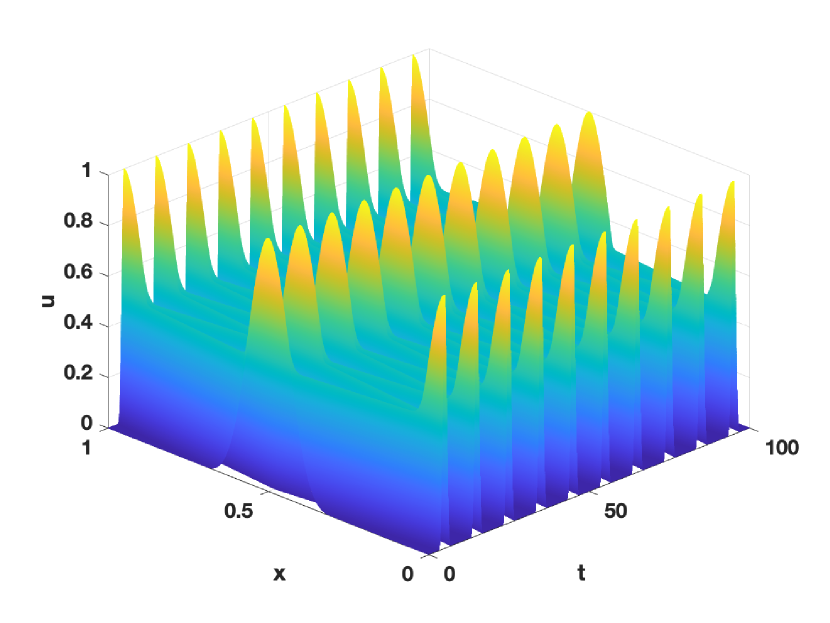
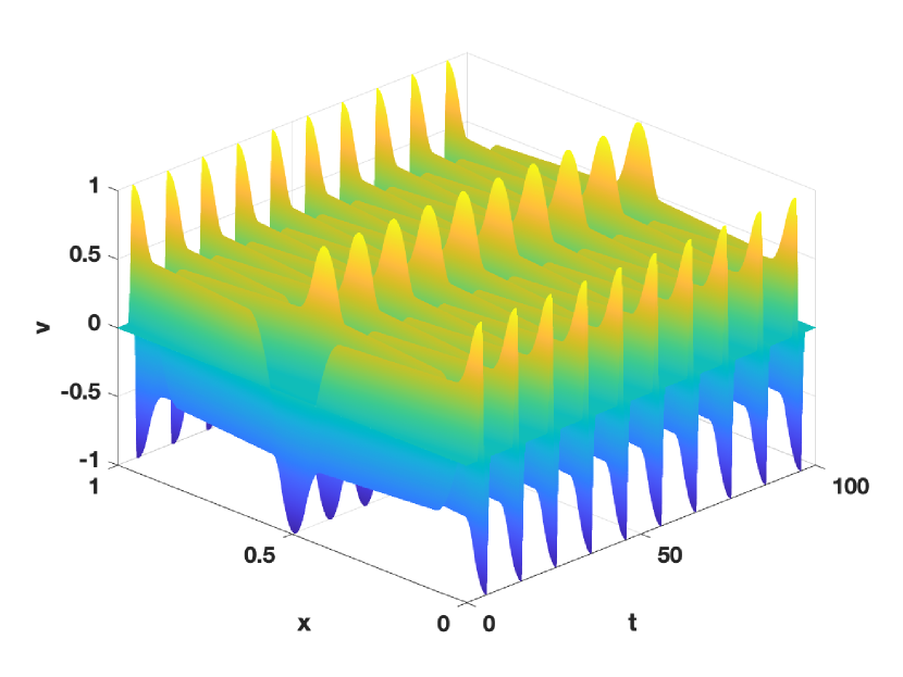
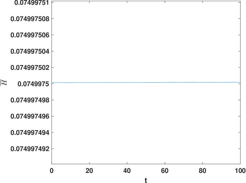
Figure 1: (Wave Equation) Full-order model simulation when $T_{\text{FOM}}=100$: time evolution of ${\mathbf{u}}$ (left), ${\mathbf{v}}$ (middle), and energy $\overline{H}(t)$ (right).

Note that the Hamiltonian energy is preserved as $\overline{H}(t)\approx 7.5\times 10^{-2}$.

ROM construction

We assemble the snapshot matrices ${\mathbf{U}}$ and ${\mathbf{V}}$ from full-order simulations and generate the basis matrices ${\boldsymbol{\Phi}}_{u}\in\mathbb{R}^{n\times r_{1}}$ and ${\boldsymbol{\Phi}}_{v}\in\mathbb{R}^{n\times r_{2}}$ that contain, respectively, the $r_{1}$ and $r_{2}$ leading left singular vectors of ${\mathbf{U}}$ and ${\mathbf{V}}$. We define the POD basis ${\boldsymbol{\Phi}}=\left[\begin{array}[]{cc}{\boldsymbol{\Phi}}_{u}&\mathbf{0}\\ \mathbf{0}&{\boldsymbol{\Phi}}_{v}\end{array}\right]$ and obtain the projected data ${\mathbf{Y}}_{r}={\boldsymbol{\Phi}}^{\intercal}{\mathbf{Y}}={\boldsymbol{\Phi}}^{\intercal}[{\mathbf{U}}^{\intercal},{\mathbf{V}}^{\intercal}]^{\intercal}$ as well as the associated gradient of the Hamiltonian and the time derivative data matrices (using $\mathcal{D}_{t}$ defined in (11)). For simplicity, we choose $r_{1}=r_{2}=r$ in the following tests. However, different basis sizes can be chosen to better represent data. Next, we offers several comparisons of the ROMs generated by GP-OpInf, GP-OpInf-V and GP-OpInf-P and investigate their performance over $[0,T_{\text{ROM}}]$.

Test 1. Effects of regularization

We first consider the non-parametric case in which $\mu=10$ is fixed. The mesh size for the FOM is $\Delta x=10^{-3}$ (correspondingly, $n=1,000$) and the same time step $\Delta t=1\times 10^{-3}$ is used in both the FOM and the ROMs. We use GP-OpInf, GP-OpInf-V and GP-OpInf-P to create ROMs of dimension $2r$ ($r$ bases for $u$ and $r$ bases for $v$) and let $r$ vary from $r=5$ to $r=200$.

We first select $T_{\text{FOM}}=5$, $T_{\text{ROM}}=5$ and check whether the inferred ${\mathbf{D}}_{r}$ possesses the desired skew-symmetric structure by plotting the maximum magnitude of $|{\mathbf{D}}_{r}+{\mathbf{D}}_{r}^{\intercal}|$ in Figure 2 (left). The inferred ${\mathbf{D}}_{r}$ from GP-OpInf-P (with $\alpha=2$ in the definition of $\epsilon$ (17)) achieves better anti-symmetric structure than GP-OpInf-V when $r>30$, but both methods are not producing satisfactory results and are far off from being skew-symmetric. In contrast, the proposed GP-OpInf produces exact anti-symmetric matrices up to machine precision. The associated ROM approximation errors $\mathcal{E}$ are plotted in Figure 2 (right). For the GP-OpInf-V method, the error grows unbounded (no entry indicates an NaN) when $r>40$. The GP-OpInf-P method yields better performance as it provides stable numerical solutions at almost all of the considered $r$-values, yet it becomes inaccurate at $r=105$ and $r=155$. In contrast, the GP-OpInf method is able to obtain stable numerical approximations for all the $r$-values.

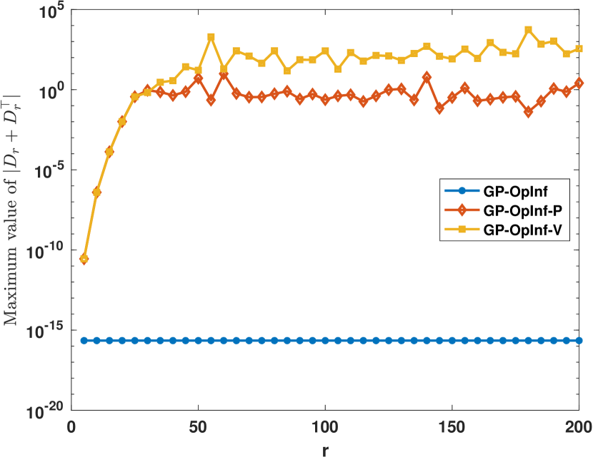
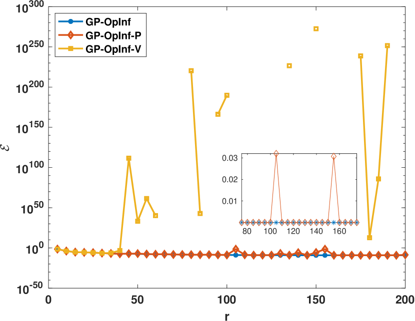
Figure 2: (Wave Equation) ROMs of $2r$-dimensions when $T_{\text{FOM}}=5$ and $T_{\text{ROM}}=5$: (left) maximum magnitude of $|{\mathbf{D}}_{r}+{\mathbf{D}}_{r}^{\intercal}|$ for the inferred ${\mathbf{D}}_{r}$ when $r$ varies; (right) ROM approximation error $\mathcal{E}$ from (30) when $r$ varies from 5 to 200 in increments of five. The inserted plots cover the portion of $r$ between 75 and 175.

We now consider the case of $T_{\text{FOM}}=10$ and $T_{\text{ROM}}=10$. The associated maximum magnitude of $|{\mathbf{D}}_{r}+{\mathbf{D}}_{r}^{\intercal}|$ and the approximation errors of the ROMs based on three inferred ${\mathbf{D}}_{r}$ are plotted in Figure 3. From the results, we find that all three methods learn ${\mathbf{D}}_{r}$ with skew-symmetric structure, however, with noticeable differences. The maximum magnitude of $|{\mathbf{D}}_{r}+{\mathbf{D}}_{r}^{\intercal}|$ is about $10^{-6}$ in GP-OpInf-V and GP-OpInf-P. Once again GP-OpInf is the most accurate yielding machine precision, $10^{-16}$, for the skew-symmetry test. From Figure 3 (right), we observe that the three ROMs yield similar numerical accuracy in this case.

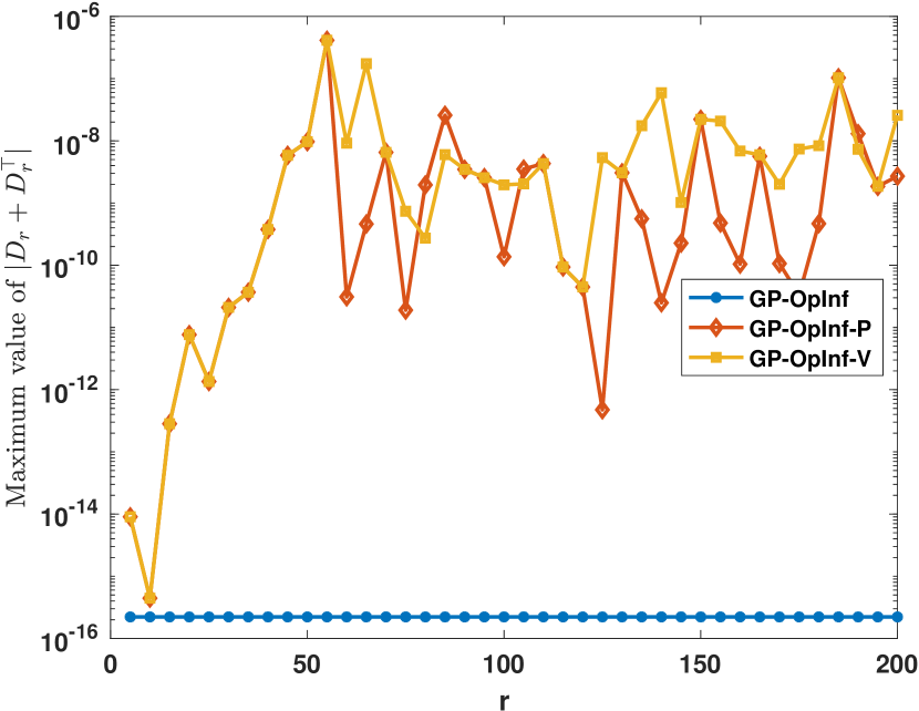
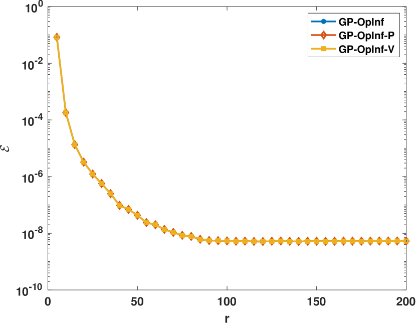
Figure 3: (Wave Equation) ROMs of $2r$-dimensions when $T_{\text{FOM}}=10$ and $T_{\text{ROM}}=10$: (left) maximum magnitude of $|{\mathbf{D}}_{r}+{\mathbf{D}}_{r}^{\intercal}|$ for the inferred ${\mathbf{D}}_{r}$ when $r$ varies; (right) numerical error $\mathcal{E}$ from (30) when $r$ varies from 5 to 200 in increments of five.

In sum, we find that the GP-OpInf approach achieves ${\mathbf{D}}_{r}$ with skew-symmetric structure up to machine precision in both tests, which is markedly better than GP-OpInf-V and GP-OpInf-P. While more training data improved the GP-OpInf-V and GP-OpInf-P structural properties, noticeable (10 orders of magnitude) differences remained. The resulting GP-OpInf ROMs are more accurate, which is especially evident in the first test case where the other two approaches failed. In the following tests, we thus only focus on the GP-OpInf approach and investigate it in more detail.

Test 2. Illustration of error estimation

Here, we investigate the error estimation for the GP-OpInf ROM for the same non-parametric case with $\mu=10$, and compare the approximation error with the intrusive structure-preserving ROM (SP-G ROM) of the same dimension.

We choose $\Delta x=\Delta t=2\times 10^{-4}$ so that the discretization errors are negligible relative to the POD projection error and the optimization error. We set $T_{\text{FOM}}=T_{\text{ROM}}=10$ and vary the dimension $r$ of the ROM. The three ROM errors (30)–(32) are plotted in Figure 4 (left), which shows that the error decays monotonically as $r$ increases. When $r>200$, the ROM approximation error saturates, although the POD projection error is still decreasing, which indicates the error is dominated by the saturated optimization error and the fixed time discretization error. We compare the GP-OpInf ROM approximation error with the SP-G ROM in Figure 4 (right). The SP-G approximation error decreases in a tendency similar to the POD projection error in Figure 4 (left), and GP-OpInf achieves similar numerical accuracy to SP-G when $r$ is less than 200. However, as $r$ increases, the GP-OpInf ROM approximation accuracy stays around $10^{-8}$. Nevertheless, such large $r$ values lead to impractically expensive ROMs, and are of little practical use.

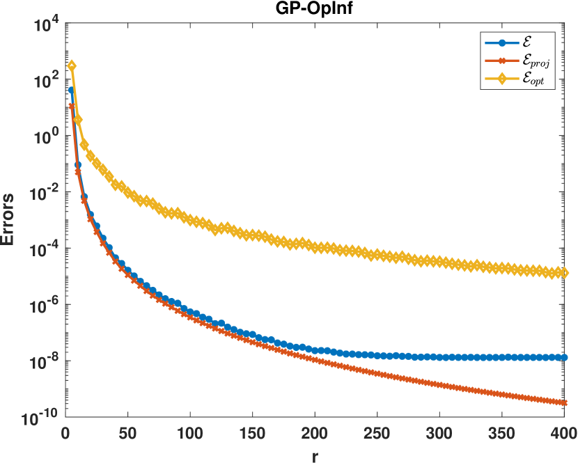
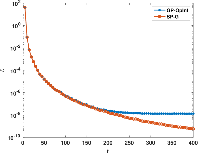
Figure 4: (Wave Equation) Numerical errors of the $2r$-dimensional GP-OpInf ROM when $T_{\text{FOM}}=T_{\text{ROM}}=10$ and $\Delta x=\Delta t=2\times 10^{-4}$: (left) the ROM approximation error (30) together with POD projection error (31) and optimization error (32); (right) comparison of the ROM approximation error for the GP-OpInf and SP-G ROM.

In this numerical test, $T_{\text{FOM}}=T_{\text{ROM}}$, as assumed when deriving the error estimation. Since Operator Inference is a data-driven technique, the optimization error and POD projection error depend on the given snapshot data. Consequently, there is no general accuracy guarantee for the ROM simulations beyond the time duration on which the snapshots are gathered. Nonetheless, if the snapshot data represent the dynamical system behavior well, it is possible to attain accurate ROM predictions. Nevertheless, the predictive capabilities of the ROMs outside the training intervals are enhanced by enforcing the correct structure in the inferred ROMs. We investigate predictions for longer time intervals in the next test.

Test 3. Long-term predictive capabilities of the GP-OpInf ROM

We set $\Delta x=\Delta t=10^{-3}$ and fix $\mu=10$ and generate snapshots from the FOM with the final time $T_{\text{FOM}}=10$. However, we simulate the GP-OpInf ROM on a much longer interval with $T_{\text{ROM}}=100$ to demonstrate the long-term predictive capabilities of structure-preserving ROMs. The time evolution of the ROM approximation errors, using the FOM solution as the benchmark, at $r=10,20,40$ and $80$ are plotted in Figure 5 (left). The associated approximate Hamiltonian values are plotted in Figure 5 (right), where the dashed line indicates the end of the training time interval. We observe that for $r=10$ and $20$, the errors stay at the same level over time, while for $r=40$ and $80$, the errors increases gradually as $t$ increases. Meanwhile, since the appropriate (gradient) structure is captured in the inferred GP-OpInf ROM, the approximate Hamiltonian is conservative, which approaches the benchmark value (from the FOM) as $r$ increases. We remark that these Hamiltonian approximations can be improved by choosing $\overline{{\mathbf{y}}}={\mathbf{y}}^{0}$ and using a POD basis generated from the shifted snapshots as introduced in [26].

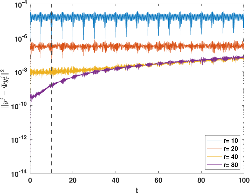
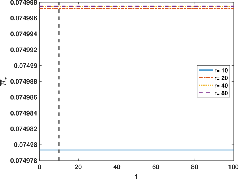
Figure 5: (Wave Equation) Numerical accuracy of the $2r$-dimensional GP-OpInf: (left) time evolution of the summand of the ROM approximation error (30); (right) time evolution of the reduced-order approximate Hamiltonian energy. The dashed line indicates the end of the training interval.

Test 4. Parametric predictions away from training data

We parameterize the initial condition $u_{0}(x;\mu)=h(s(x;\mu))$ and let $\mu\in[5,15]$. To generate snapshots, 11 uniformly distributed training samples are collected from the parameter interval and the FOM is simulated at all samples with $\Delta x=\Delta t=10^{-3}$ and $T_{\text{FOM}}=10$. Then, we compute the POD basis from the collected snapshots, learn the GP-OpInf ROM, from which we predict solutions at different test parameters over the same time interval ($T_{\text{ROM}}=T_{\text{FOM}}$). We consider three randomly selected test parameters, $\mu=6.7,9.5$ and $14.1$.

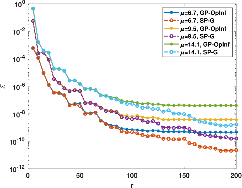
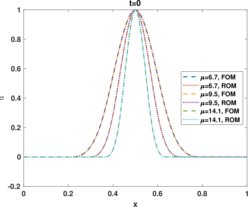
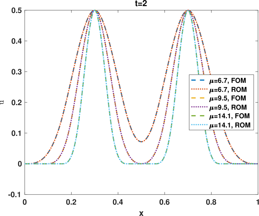
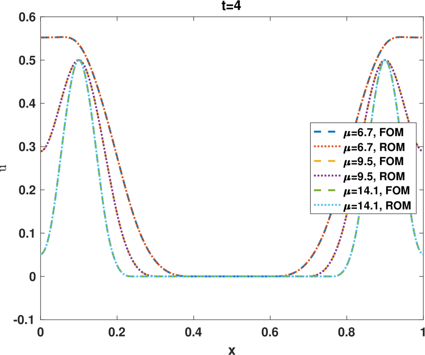
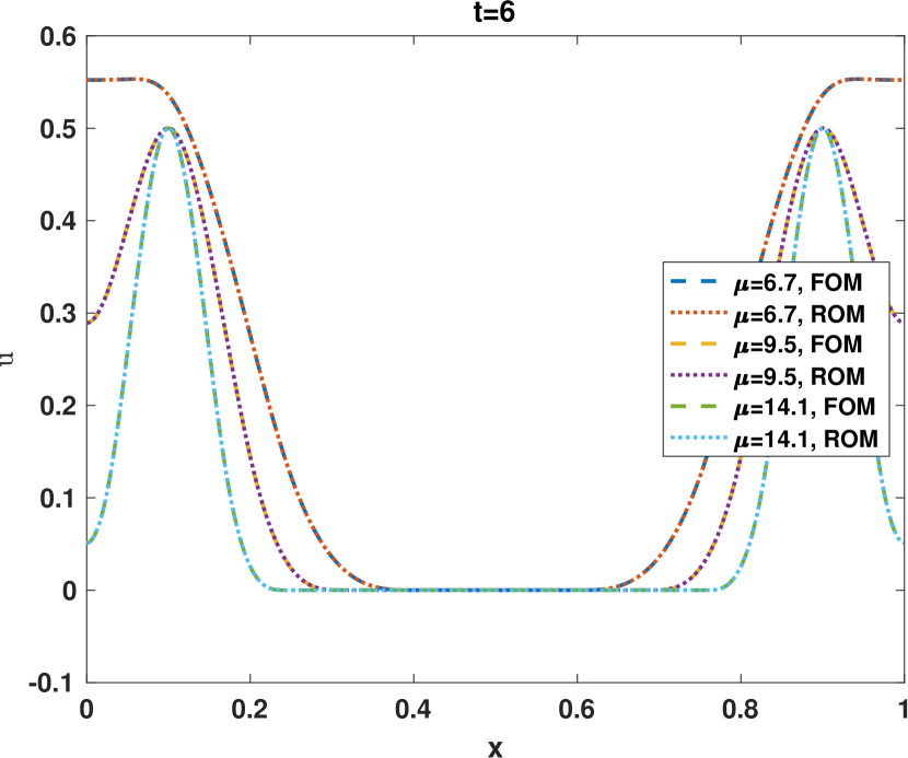
Figure 6: (Wave Equation) Performance at three test parameters: (left) comparison of the ROM approximation errors (30) for the GP-OpInf with the SP-G ROM of the same dimension $2r$; (right) the GP-OpInf ROM solution and the FOM solution at $t=0,2,4,6$.

Figure 6 (left) compares the approximation errors of the SP-G ROM and the GP-OpInf. The figure shows that at all test parameters $\mu$, the error of the GP-OpInf ROM is close to that of SP-G ROM when $r\leq 80$. The error, however, saturates when $r$ becomes bigger and, thus, turns larger than that of the SP-G ROM. Nevertheless, such large basis dimensions produce inefficient ROMs and are of little practical value. We choose the more realistic $r=40$ case and plot the benchmark FOM solution and the ROM solution in Figure 6 (right); only a few snapshots are shown for illustration. In each case, the GP-OpInf ROM achieves accurate approximations close to the FOM solution.

5.2.2 Parameterized Korteweg-de Vries (KdV) equation

Next, we consider the one-dimensional KdV equation

$$u_{t}=\alpha uu_{x}+\nu u_{xxx},\quad(x,t)\in\Omega\times I,$$

where $u=u(x,t;\mu)$ is the parameter-dependent solution and $\mu\in P$ a parameter appearing in the initial condition, defined below alongside the boundary and initial conditions. The KdV equation can be rewritten as a non-canonical Hamiltonian system (see, e.g., [16]):

$$u_{t}=\mathcal{S}\frac{\delta\mathcal{H}}{\delta u},$$

where $\mathcal{S}=\partial_{x}$ denotes the first-order derivative operator with respect to space, and the Hamiltonian function $\mathcal{H}(u)=\int_{\Omega}\left(\frac{\alpha}{6}u^{3}-\frac{\nu}{2}u_{x}^{2}\right)\,{\rm d}x$. After taking a spatial discretization with a uniform mesh size $\Delta x$ and defining a consistent discrete Hamiltonian $\overline{H}(t)\coloneqq\Delta xH({\mathbf{u}})$ with $H({\mathbf{u}})=\sum_{j}\left[\frac{\alpha}{6}u_{j}^{3}-\frac{\nu}{2}(u_{j+1}-u_{j})^{2}\right]$, we obtain the semi-discrete Hamiltonian system

$$\accentset{\mbox{\large.}}{{\mathbf{u}}}={\mathbf{A}}\left(\frac{\alpha}{2}{\mathbf{u}}^{2}+\nu{\mathbf{B}}{\mathbf{u}}\right),$$ (34)

where ${\mathbf{A}}$ and ${\mathbf{B}}$ are the matrices associated to the discretization of the skew-adjoint operator $\mathcal{S}$ and the second-order derivative by central differences, respectively. Since ${\mathbf{A}}$ is skew-symmetric, this dynamical system conserves the discrete Hamiltonian $\overline{H}(t)$.

Computational setting

We set $\Omega=[-20,20]$, $\alpha=-6$, $\nu=-1$, and consider periodic boundary conditions $u(-20,t;\mu)=u(20,t;\mu)$ for any $t\in I$ and we parameterize the initial condition $u_{0}(x;\mu)=\text{sech}^{2}\left(\frac{x}{\mu}\right)$, for any $\mu\in{P}=[1,5]$. In the FOM (34), we have

$${\mathbf{A}}=\frac{1}{2\Delta x}\mathbf{S}_{n},\quad\text{and}\quad{\mathbf{B}}=\frac{1}{\Delta x^{2}}\mathbf{L}_{n}.$$

The mesh size $\Delta x=0.01$ (correspondingly, $n=4,000$) is used in all simulations. For time integration, we use the average vector field (AVF) method together with a Picard iteration to solve the nonlinear system.

When $T_{\text{FOM}}=20$, $\Delta t=0.01$ and $\mu=\sqrt{2}$, the time evolution of the full-order state and approximate Hamiltonian $\overline{H}(t)$ are shown in Figure 7. We observe that the system is conservative, with the Hamiltonian staying around $\overline{H}(t)\approx-1.13$ during the simulation.

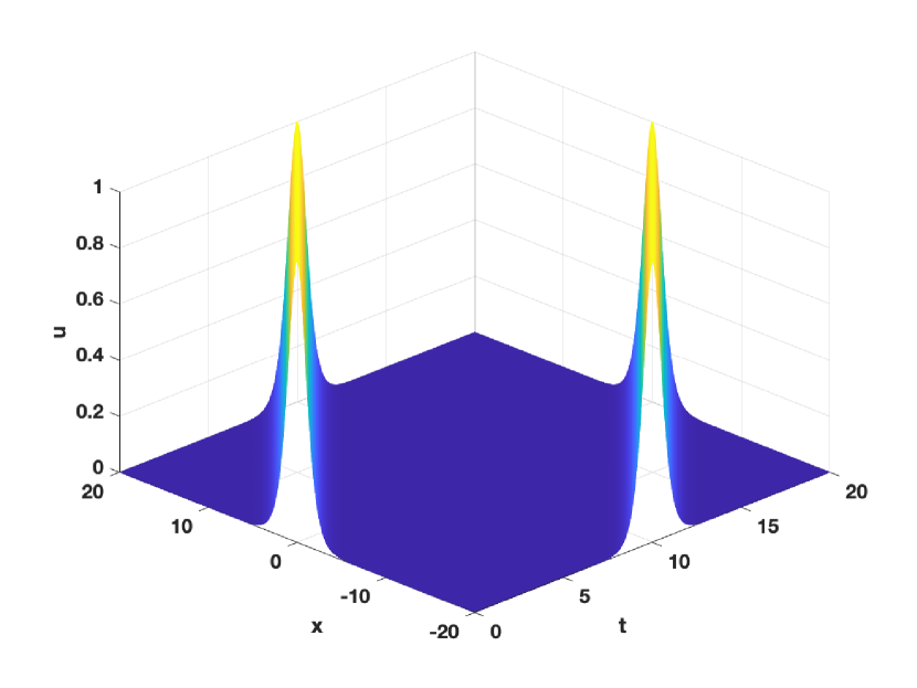
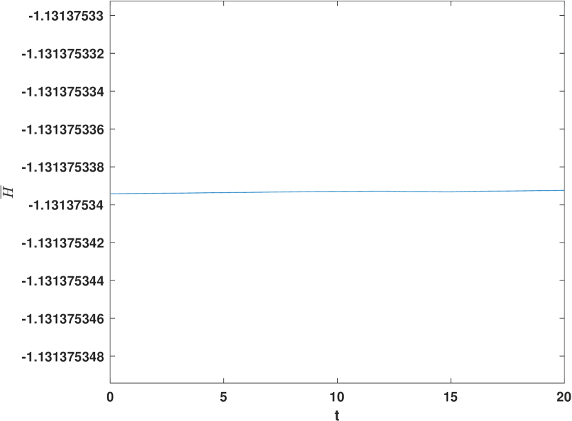
Figure 7: (KdV Equation) Full-order model simulation up to final time $T_{\text{FOM}}=20$: time evolution of ${\mathbf{u}}$ (left) and approximate Hamiltonian $\overline{H}(t)$ (right).

Test 1. Illustration of error estimation

We demonstrate the estimation of the GP-OpInf ROM approximation error in a non-parametric case with $\mu=\sqrt{2}$, and compare the approximation error with the SP-G ROM of the same dimension. To verify the error estimation, we choose a small time step $\Delta t=2.5\times 10^{-3}$, let $T_{\text{FOM}}=T_{\text{ROM}}=20$ and vary the dimension of the ROM. Figure 8 (left) shows the three error measures from equations (30)–(32). The ROM approximation error decays monotonically until $r>80$ and then levels off. The optimization error follows a similar trend, yet the projection error continues to decay until $r\approx 170$. Figure 8 (right) compare the GP-OpInf ROM approximation error with that of the SP-G ROM. We observe that SP-G and GP-OpInf achieve the same accuracy for $r<70$, which covers the model dimension where most practical ROMs would be selected from, whereas for larger $r$ the SP-G ROM performs better.

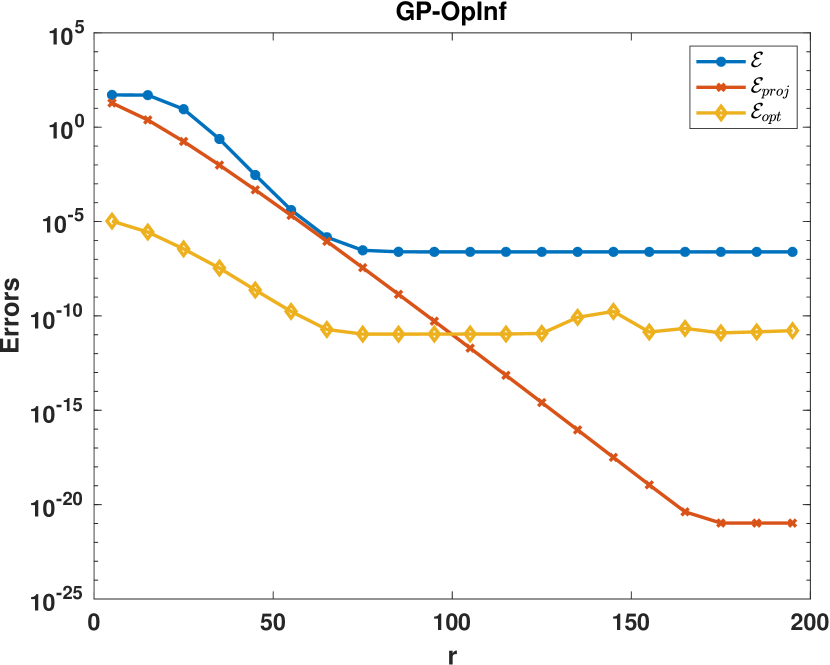
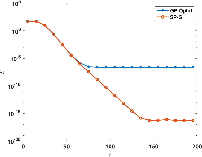
Figure 8: (KdV Equation) Numerical errors of the $r$-dimensional GP-OpInf ROM when $T_{\text{FOM}}=T_{\text{ROM}}=20$ and $\Delta t=2.5\times 10^{-3}$: (left) the ROM approximation error (30) together with POD projection error (31) and optimization error (32); (right) comparison of the ROM approximation error of the GP-OpInf ROM with the SP-G ROM.

Test 2. Long-term predictive capabilities of the GP-OpInf ROM

We set $\Delta t=10^{-2}$ and fix $\mu=\sqrt{2}$ and generate snapshots from FOM with the final time $T_{\text{FOM}}=20$. We simulate the GP-OpInf ROM 100% past the training interval, so $T_{\text{ROM}}=40$. Figure 9 (left) shows the time evolution of the ROM approximation errors at $r=10,20,40$ and $80$, where the FOM solution is the benchmark. The associated approximate Hamiltonian values are plotted in Figure 9 (right), where the dashed line indicates the end of the training interval. The errors increase gradually as $t$ increases due to usual error accumulation. Since the appropriate (gradient) structure is captured in the inferred GP-OpInf ROMs, the approximate Hamiltonian functions are constant and approach the benchmark value for $r$ is sufficiently large.

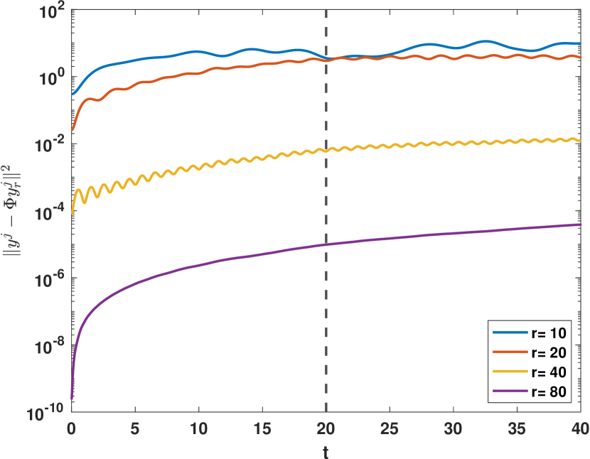
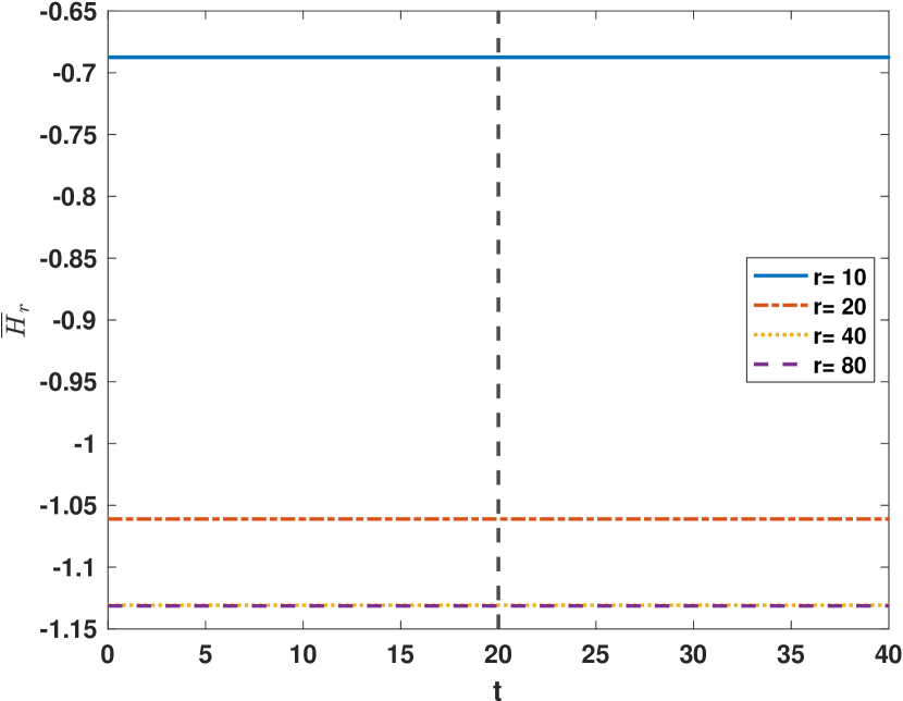
Figure 9: (KdV Equation) Numerical accuracy of the $r$-dimensional GP-OpInf ROM: (left) time evolution time evolution of the summand of the ROM approximation error (30); (right) time evolution of the values of reduced-order approximate Hamiltonian functions. The dashed line indicates the end of the training interval.

Test 3. Parametric predictions away from training data

We parameterize the initial condition as $u_{0}(x;\mu)=\text{sech}^{2}\left(\frac{x}{\mu}\right)$ for $\mu\in{P}=[1,5]$. To generate snapshots, nine training samples are uniformly collected from the interval and the FOM is simulated at all samples with $\Delta t=10^{-2}$ and $T_{\text{FOM}}=20$. We compute the POD basis from the collection of snapshot matrices. Next, we infer the GP-OpInf ROM and use it to make predictions at the test parameters, where we keep the time interval fixed ($T_{\text{ROM}}=T_{\text{FOM}}$). We evaluate the ROMs accuracy at three randomly selected test parameters $\mu=1.4,2.8$ and $4.7$.

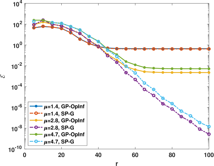
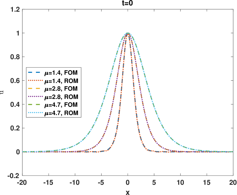
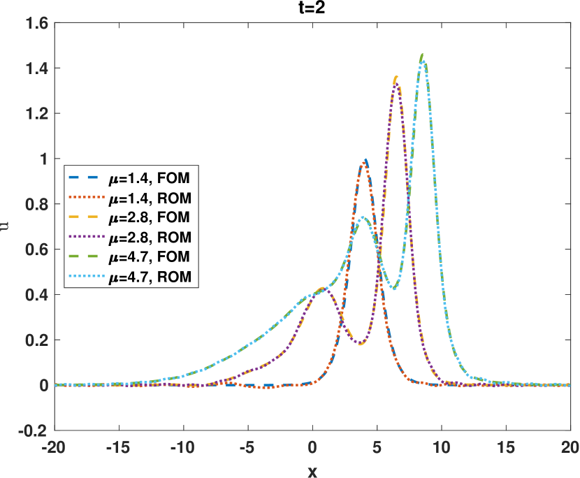
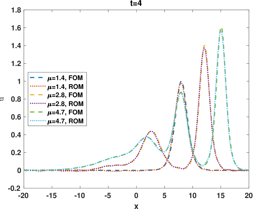
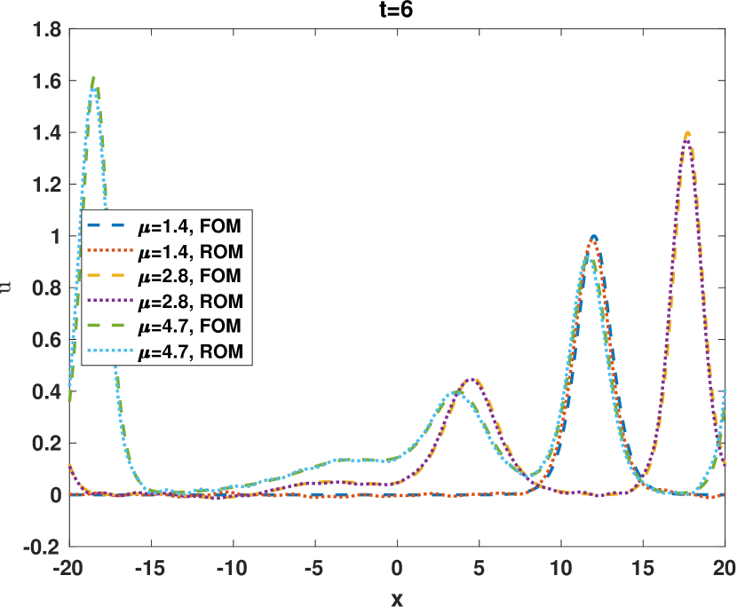
Figure 10: (KdV Equation) Performance of the $r$-dimensional GP-OpInf ROM at several test parameters: (left) comparison of the ROM approximation error (30) for the SP-G ROM of the same dimension $r$; (right) snapshots of the GP-OpInf ROM solution and the FOM solution at several time instances.

Figure 10 (left) shows a comparison of the ROM approximation errors (30) of the SP-G and the GP-OpInf ROMs. At the test parameters, the error of the GP-OpInf ROM is close to the SP-G ROM when $r\leq 50$ (which is where most practical ROM model dimensions would be selected from), yet the error saturates when $r$ gets bigger and thus becomes larger than that of SP-G. We fix $r=40$ and plot the FOM solution and the GP-OpInf ROM solution at several selected time instances in Figure 10 (right). This shows that the ROM produces accurate approximations of the FOM solution at these test parameters.

5.3 Dissipative PDEs

We consider the Allen-Cahn equation to assess the GP-OpInf ROM’s performance on a dissipative system.

5.3.1 One-dimensional Allen-Cahn equation

Consider the one-dimensional Allen-Cahn equation

$$u_{t}=\epsilon^{2}u_{xx}+(u-u^{3}),\quad(x,t)\in\Omega\times I\text{ and }\mu\in P,$$

where $u=u(x,t;\mu)$ with $\mu$ a parameter in the initial condition. The equation can be recast to the form (1), that is, $u_{t}=-\frac{\delta\mathcal{H}}{\delta u}$, with the Lyapunov function $\mathcal{H}(u)=\int_{\Omega}\left(\frac{\epsilon^{2}}{2}u_{x}^{2}-\frac{1}{2}u^{2}+\frac{1}{4}u^{4}\right)\,{\rm d}x$ (see, e.g., [16]). After applying a uniform spatial discretization with the mesh size $\Delta x$ and defining a consistent discrete Lyapunov function $\overline{H}(t)\coloneqq\Delta xH({\mathbf{u}})$ with $H({\mathbf{u}})=\sum_{j}[\frac{\epsilon^{2}}{2\Delta x^{2}}(u_{j+1}-u_{j})^{2}-\frac{1}{2}u_{j}^{2}+\frac{1}{4}u_{j}^{4}]$, we obtain the semi-discrete system

$$\accentset{\mbox{\large.}}{\mathbf{u}}=-\mathbf{I}_{n}(-\mathbf{Au}-\mathbf{u}+\mathbf{u}^{3}),$$ (35)

where ${\mathbf{I}}_{n}$ is the $n\times n$ identity matrix, ${\mathbf{A}}$ is associated to a discrete, one-dimensional, second-order differential operator, and $\mathbf{u}^{3}$ is the component-wise cubic function of the vector $\mathbf{u}$. Since $-{\mathbf{I}}_{n}$ is negative definite, the Lyapunov function decreases in time.

Computational setting

Set $\Omega=[-1,1]$, the interface parameter $\epsilon=0.01$, and consider periodic boundary conditions $u(-1,t;\mu)=u(1,t;\mu)$ and $\frac{\partial u}{\partial\mathbf{n}}(-1,t;\mu)=\frac{\partial u}{\partial\mathbf{n}}(1,t;\mu)$ for $t\in I$. The initial condition is $u_{0}(x;\mu)=\mu x^{2}\sin(2\pi x)$, for $\mu\in{P}=[0.2,2]$ (see [67] for numerical simulations of a non-parametric configuration). In the FOM (35), we have

$${\mathbf{A}}=\frac{\epsilon^{2}}{\Delta x^{2}}\mathbf{L_{n}}.$$

In all full-order simulations, we choose the mesh size $\Delta x=10^{-3}$ and use the AVF method for time integration with a time step size $\Delta t$. To solve the nonlinear systems of equations, we apply Picard iteration. Figure 11 shows the time evolution of the full-order state and discrete Lyapunov function $\overline{H}(t)$ where we set $\mu=1$, $T_{\text{FOM}}=5$ and $\Delta t=10^{-3}$.

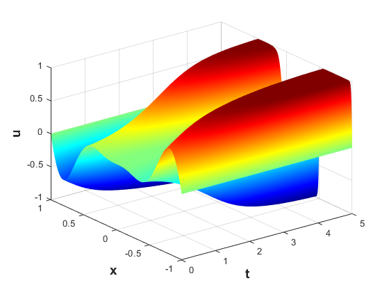
Figure 11: (1D Allen-Cahn Equation) Full-order model simulation with final time $T_{\text{FOM}}=5$: time evolution of the state ${\mathbf{u}}$ (left) and the approximate Lyapunov function $\overline{H}(t)$ (right).

Test 1. Illustration of error estimation

We set $T_{\text{FOM}}=T_{\text{ROM}}=3$, fix the parameter $\mu=1$, and choose a small time step $\Delta t=2.5\times 10^{-4}$ so that the time discretization error is negligible in the error estimate. Varying the dimension $r$ of the ROM, we compute the GP-OpInf ROM approximation error (30), optimization error (32) and projection error (32), which are shown in Figure 12 (left). In this case, for $r\leq 15$, the optimization error is smaller than the POD projection error; however, for a bigger $r$, the former becomes larger and levels off. Correspondingly, the GP-OpInf ROM approximation error first decreases monotonically and then reaches a plateau. Therefore, compared to the SP-G ROM, the GP-OpInf ROM achieves the same accuracy for small $r$, but yields larger numerical error when its dimension is large, as shown in Figure 12 (right).

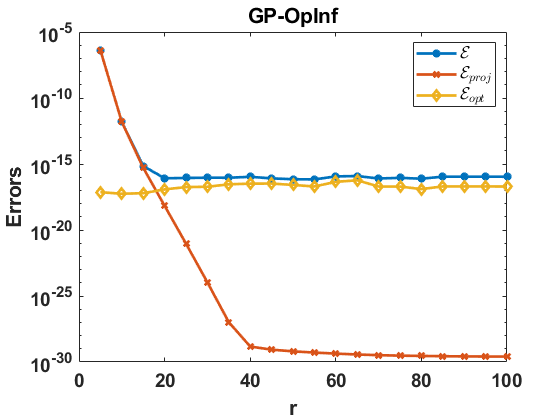
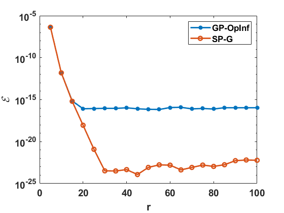
Figure 12: (1D Allen-Cahn Equation) Numerical errors for the $r$-dimensional GP-OpInf when $T_{\text{FOM}}=T_{\text{ROM}}=3$ and $\Delta t=2.5\times 10^{-4}$: (left) the ROM error together with the POD projection error (31) and the optimization error (32); (right) comparison of the GP-OpInf ROM approximation error (30) with that of the SP-G ROM.

Test 2. Prediction-in-time capabilities of the GP-OpInf ROM

Setting $\Delta t=10^{-3}$, we generate snapshots from the full-order simulation with the final time $T_{\text{FOM}}=3$ and simulate the ROM to the final time $T_{\text{ROM}}=5$, which is 66% past the training data. The ROM approximation errors (30) at $r=10,20,40$ and $80$ are plotted in Figure 13 (left) alongside the FOM solutions. The associated approximate Lyapunov function is plotted in Figure 13 (right). The dashed line indicates the end of the training time interval. It is evident that the ROM is accurate within the interval $[0,3]$, but its accuracy degrades when the simulation time exceeds this range. Meanwhile, the approximate Lyapunov is decreasing in time as guaranteed by the gradient structure of the ROM.

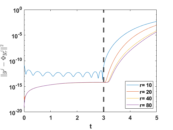
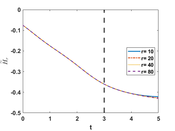
Figure 13: (1D Allen-Cahn Equation) Numerical accuracy of the $r$-dimensional GP-OpInf ROM: (left) time evolution time evolution of the summand of the ROM approximation error (30); (right) time evolution of the reduced-order approximate Lyapunov function. The dashed line indicates the end of the training interval.

Test 3. Parametric predictions away from training data

We parameterize the problem with the interface parameter $\mu\in{P}=[0.2,2]$, which also affects the initial condition. To generate snapshots, we simulated the FOM at 10 uniformly distributed training parameter samples in ${P}$ with the time step $\Delta t=10^{-3}$ and final simulation time $T_{\text{FOM}}=3$. We construct the GP-OpInf ROM from the collected snapshot data and use it to obtain predictions at any given test parameter over the same time interval ($T_{\text{ROM}}=T_{\text{FOM}}$). Here, we select three random test parameters, $\mu=0.34,0.96$ and $1.87$.

Figure 14 (left) shows the approximation errors of the SP-G and GP-OpInf ROMs. This illustrates that, at all test parameters, the error of GP-OpInf is close to that of SP-G when $r\leq 30$. The former levels off at values around $10^{-15}$ when $r$ becomes large, which is well beyond a typically required accuracy. Therefore, the GP-OpInf is very accurate. Figure 14 (right) compares the FOM solution with the GP-OpInf ROM solution of dimension $r=30$ at several time instances. This confirms that the GP-OpInf ROM provides an accurate approximation to the FOM solution in all cases.

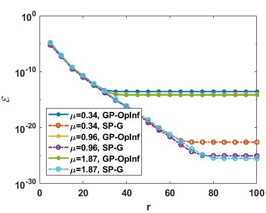
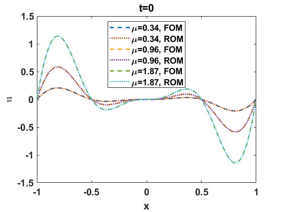
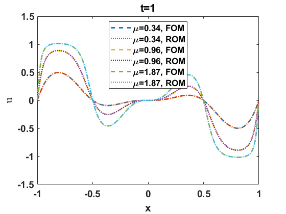
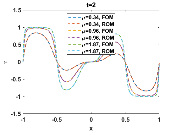
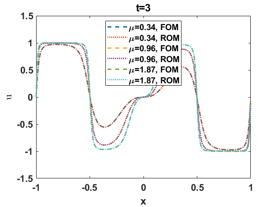
Figure 14: (1D Allen-Cahn Equation) Performance of $r$-dimensional GP-OpInf ROM: (left) comparison of the ROM approximation error (30) for the SP-G ROM in problems with different $\mu$; (right) snapshots of the ROM and FOM solutions at several time instances.

5.3.2 Two-dimensional parameterized Allen-Cahn equation

Consider the two-dimensional Allen-Cahn equation on a rectangular domain $\Omega$:

$$u_{t}=\epsilon^{2}\Delta u+u-u^{3},\quad(x,y)\in\Omega,t\in I,$$

where $u=u(x,t;\mu)$ is the parameter-dependent solution and $\mu\in P$ a parameter appearing in the initial condition, defined below alongside the boundary and initial conditions. The Allen-Cahn equation can be recast into the form (1), in a similar way as in the 1D case, with the Lyapunov function $\mathcal{H}(u)=\int_{\Omega}\left(\frac{\epsilon^{2}}{2}|\nabla u|^{2}-\frac{1}{2}u^{2}+\frac{1}{4}u^{4}\right)\,{\rm d}x$. Let ${\mathbf{u}}$ be a vectorization of the approximate state defined on the rectangular grid, obtained by applying a spatial discretization with a uniform mesh size $\Delta x$ and $\Delta y$ in the horizontal and vertical directions. The semi-discrete system is then

$$\mathbf{\accentset{\mbox{\large.}}{u}}=-\mathbf{I}_{n^{2}}(-\epsilon^{2}\mathbf{L}\mathbf{u}-\mathbf{u}+\mathbf{u}^{3}),$$

where $\mathbf{L}=\mathbf{I}_{n}\otimes{\mathbf{D}}_{x}^{2}+{\mathbf{D}}_{y}^{2}\otimes\mathbf{I}_{n}$ with ${\mathbf{D}}_{x}^{2}=\frac{1}{(\Delta x)^{2}}\mathbf{L}_{n}$, ${\mathbf{D}}_{y}^{2}=\frac{1}{(\Delta y)^{2}}\mathbf{L}_{n}$ and $\otimes$ denotes the Kronecker product [14].

Computational setting

Let the problem be defined on $\Omega=[-0.5,0.5]^{2}$ and $I=[0,T_{\text{FOM}}]$. Consider a periodic boundary condition and $\epsilon=0.02$. The initial condition (following [25]) is given by

$$u_{0}(x,y;\mu)=\max\left(\tanh\left(\frac{r-\sqrt{(x-r(0.7-\mu))^{2}+(y+r\mu)^{2}}}{\epsilon}\right),\tanh\left(\frac{r-\sqrt{(x+r(0.7-\mu))^{2}+(y-r\mu)^{2}}}{\epsilon}\right)\right)$$

with $r=0.2$ and $\mu$ a parameter in ${P}=[0,0.7]$. The initial condition has two disks centered at $((0.7-\mu)r,-\mu r)$ and $(-(0.7-\mu)r,\mu r)$ with radius $r$. In all FOM simulations, the spatial domain is partitioned by a rectangular grid with the mesh size $\Delta x=\Delta y=2^{-6}$ and the AVF method is used for time integration with a time step $\Delta t$. The nonlinear system is solved by the Picard iteration.

Figure 15 shows the time evolution of the FOM state and the discrete Lyapunov function $\overline{H}(t)$ when $T_{\text{FOM}}=100$, $\Delta t=1\times 10^{-2}$ and $\mu=0$.

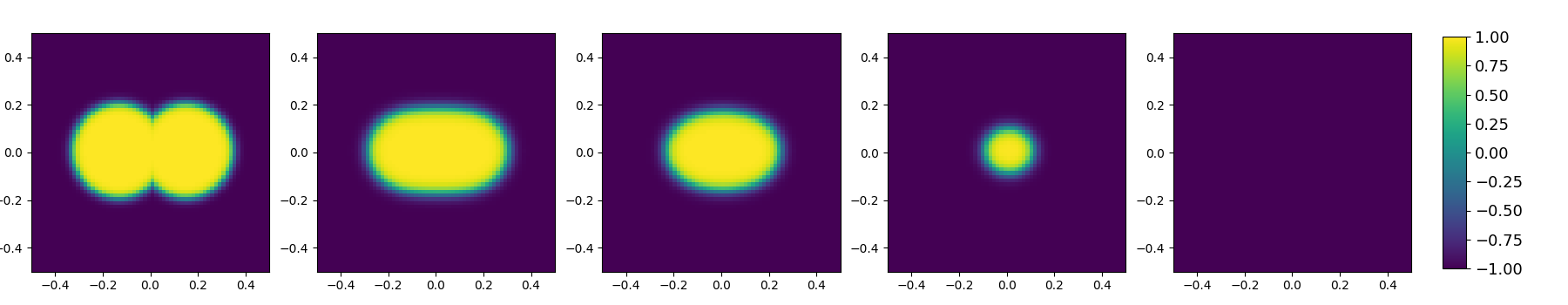
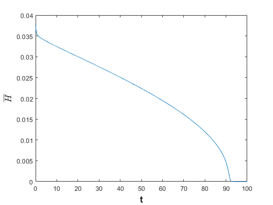
Figure 15: (2D Allen-Cahn Equation) Full-order simulation when $T_{\text{FOM}}=100$ and $\Delta t=10^{-2}$: (top) approximate states at $t=0,20,40,80,100$; (bottom) time evolution of the discrete Lyapunov function.

Similar to the 1D Allen-Cahn equation discussed in Section 5.3.1, we investigated the performance of the GP-OpInf ROM for 2D Allen-Cahn equation through three tests where we illustrate the error estimation, evaluate the GP-OpInf’s capability for time prediction, and examine parametric predictions beyond the training data. We observed that the numerical behaviors of the GP-OpInf ROM for the 2D Allen-Cahn equation closely align with those reported for the 1D case. Therefore, in the sequel, we only present the numerical test on the parametric problem in which $T_{\text{FOM}}=T_{\text{ROM}}=20$ and $\Delta t=10^{-2}$.

Test 1. Parametric predictions away from training data

To generate snapshots, 15 training samples are uniformly selected form ${P}$. The GP-OpInf ROM is then inferred from the data and used to predict solutions at any given testing samples from ${P}$. Here, the approximation errors of SP-G and GP-OpInf at three test parameters $\mu=0.17,0.38$ and $0.63$ are compared in Figure 16 (left). The figure shows that the error of GP-OpInf is close to that of SP-G with the same dimension $r$ at all test parameters. As indicated in Figure 16 (right), the optimization error is significantly lower than the POD projection error, thereby aligning the trends of errors for both GP-OpInf and SP-G with the POD projection error. Fixing $r=40$, we plot the ROM solutions and associated absolute errors at time instances $t=0,5,10,15,20$ in Figure 17. We observe that the GP-OpInf ROM produces accurate solutions for the parametric problem at the selected testing samples.

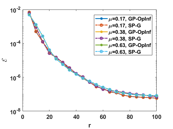
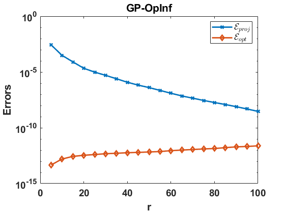
Figure 16: (2D Allen-Cahn Equation) Numerical errors for the $r$-dimensional GP-OpInf ROM: (left) comparison of the GP-OpInf ROM approximation error (30) with that of the SP-G ROM; (right) the projection error (31) and optimization error (32).

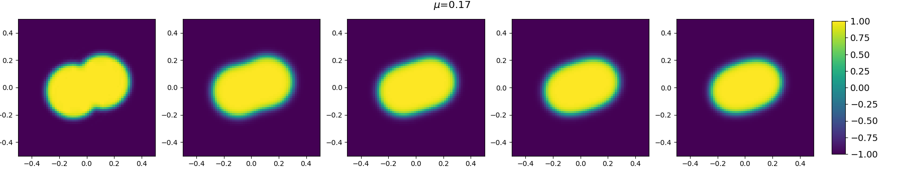
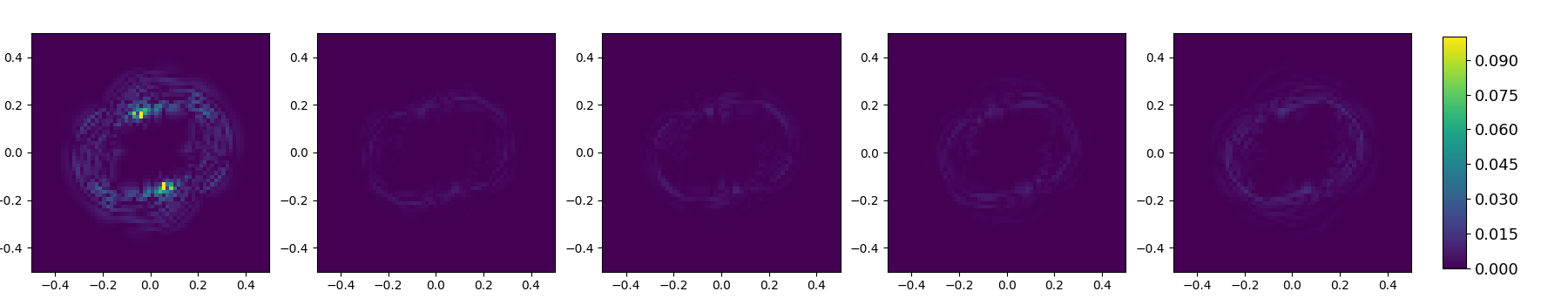
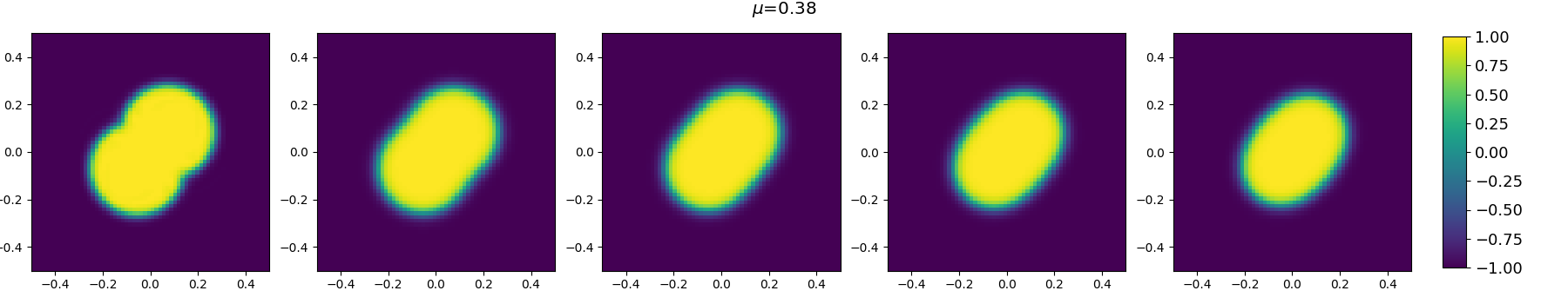
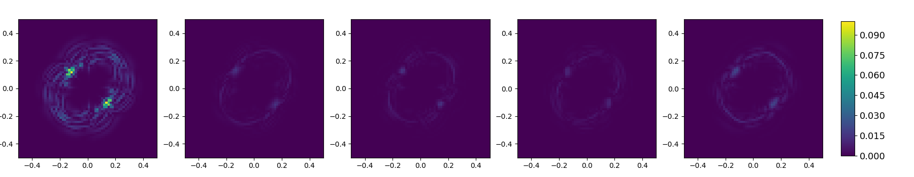
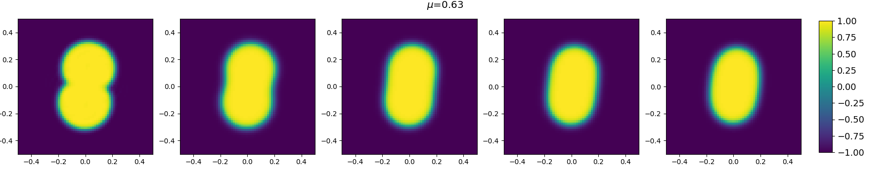
Figure 17: (2D Allen-Cahn Equation) The GP-OpInf ROM of ($r=40$) approximate solution (displayed in odd rows) and the associated approximation error $|{\mathbf{y}}(t,\mu)-{\mathbf{y}}_{r}(t,\mu)|$ (displayed in even rows) when $\mu=0.17,0.38$ and $0.63$, respectively, and $t=0,5,10,15,20$ (from left to right).

6 Conclusions

In this work, we considered evolutionary PDEs with a gradient structure with the goal to infer reduced-order models with the same gradient structure from simulated data of the semi-discretized PDEs. We first projected the high-dimensional snapshot data onto a POD basis, and from the projected data we infer a low-dimensional operator by solving a constrained optimization problem. The resulting operators then define a low-dimensional model, termed the the gradient-preserving Operator Inference (GP-OpInf) ROM. By enforcing the proper constraints in the inference of the low-dimensional operators, we ensure that the GP-OpInf ROM has the appropriate gradient structure, thereby preserving the essential physics in the reduced-order dynamics. We further analyzed the associated approximation error of the GP-OpInf ROM. The analysis shows that an upper bound for the error consists of the combination of the POD projection error, the data error and the OpInf optimization error. We test the accuracy, structure-preservation properties, and predictive capabilities of the GP-OpInf ROM on several PDE examples. For conservative test cases we consider the parameterized wave equation and Korteweg-de-Vries equation, and for dissipative test cases we consider the one-and two-dimensional Allen-Cahn equation. The numerical experiments show that GP-OpInf can achieve the same performance as the intrusive, projection-based ROM when the optimization error and data error are dominated by the POD projection error, which is typically true if the dimension of ROM is low. This observation aligns with our error estimation. Moreover, for parametric problems, the low-dimensional GP-OpInf ROMs can attain accuracy close to that of the full-order simulations even for unseen parameters.

Appendix A Iterative algorithm for solving (22)

To solve (22) , we first find the gradient of the objective function. The barrier function $g({\mathbf{X}})$ can be written as follows.

$$g({\mathbf{X}})=\sum_{i=1}^{r}\log(-\lambda_{i}({\mathbf{X}}))=\log\left(\prod_{i=1}^{r}(-\lambda_{i}({\mathbf{X}}))\right)=\log((-1)^{r}det({\mathbf{X}})).$$

Without loss of generality, we consider an even $r$ here. Differentiating it with respect to the $ij$ entry yields

$$\frac{\partial\log(det({\mathbf{X}}))}{\partial{\mathbf{X}}_{ij}}=\frac{1}{det({\mathbf{X}})}\frac{\partial det({\mathbf{X}})}{\partial{\mathbf{X}}_{ij}}.$$

Based on the cofactor formula for determinant, $det({\mathbf{X}})=\sum_{k=1}^{s}{\mathbf{X}}_{ik}{\mathbf{C}}_{ik}$, we have

$$\frac{\partial det({\mathbf{X}})}{\partial{\mathbf{X}}_{ij}} =\frac{\partial(\sum_{k=1}^{r}{\mathbf{X}}_{ik}{\mathbf{C}}_{ik})}{\partial{\mathbf{X}}_{ij}}=\sum_{k=1}^{s}\left(\frac{\partial{\mathbf{X}}_{ik}}{{\mathbf{X}}_{ij}}{\mathbf{C}}_{ik}+{\mathbf{X}}_{ik}\frac{\partial{\mathbf{C}}_{ik}}{\partial{\mathbf{X}}_{ij}}\right)={\mathbf{C}}_{ij}.$$

Therefore, we have

$$\frac{\partial\log(det({\mathbf{X}}))}{\partial{\mathbf{X}}_{ij}}=\frac{1}{det({\mathbf{X}})}{\mathbf{C}}_{ij}.$$

Due to the fact that ${\mathbf{X}}^{-1}=\frac{1}{det({\mathbf{X}})}{\mathbf{C}}^{\intercal}$, we have $\nabla g({\mathbf{X}})={\mathbf{X}}^{-\intercal}$, and

$$\nabla g({\mathbf{D}}_{r})={\mathbf{D}}_{r}^{-\intercal}.$$ (36)

Next, $f({\mathbf{D}}_{r})$ is recast into the following form using the trace:

$$f({\mathbf{D}}_{r}) =\text{tr}\left((\accentset{\mbox{\large.}}{{\mathbf{Y}}}_{r}-{\mathbf{D}}_{r}{\mathbf{F}}_{r})(\accentset{\mbox{\large.}}{{\mathbf{Y}}}_{r}-{\mathbf{D}}_{r}{\mathbf{F}}_{r})^{\intercal}\right)$$

$$=\text{tr}\left(\accentset{\mbox{\large.}}{{\mathbf{Y}}}_{r}\accentset{\mbox{\large.}}{{\mathbf{Y}}}_{r}^{\intercal}-\accentset{\mbox{\large.}}{{\mathbf{Y}}}_{r}{\mathbf{F}}_{r}^{\intercal}{\mathbf{D}}_{r}^{\intercal}-{\mathbf{D}}_{r}{\mathbf{F}}_{r}\accentset{\mbox{\large.}}{{\mathbf{Y}}}_{r}^{\intercal}+{\mathbf{D}}_{r}{\mathbf{F}}_{r}{\mathbf{F}}_{r}^{\intercal}{\mathbf{D}}_{r}^{\intercal}\right).$$

Then the gradient of $f({\mathbf{D}}_{r})$ can be obtained as follows:

$$\nabla f({\mathbf{D}}_{r})=-\accentset{\mbox{\large.}}{{\mathbf{Y}}}_{r}{\mathbf{F}}_{r}^{\intercal}-\accentset{\mbox{\large.}}{{\mathbf{Y}}}_{r}{\mathbf{F}}_{r}^{\intercal}+({\mathbf{F}}_{r}{\mathbf{F}}_{r}^{\intercal}{\mathbf{D}}_{r}^{\intercal})^{\intercal}+{\mathbf{D}}_{r}{\mathbf{F}}_{r}{\mathbf{F}}_{r}^{\intercal}=-2(\accentset{\mbox{\large.}}{{\mathbf{Y}}}_{r}-{\mathbf{D}}_{r}{\mathbf{F}}_{r}){\mathbf{F}}_{r}^{\intercal}.$$ (37)

By combining (37) and (36) , we have

$$\nabla f_{\beta}({\mathbf{D}}_{r})=\nabla f({\mathbf{D}}_{r})-\beta\nabla g({\mathbf{D}}_{r})=-2(\accentset{\mbox{\large.}}{{\mathbf{Y}}}_{r}-{\mathbf{D}}_{r}{\mathbf{F}}_{r}){\mathbf{F}}_{r}^{\intercal}-\beta{\mathbf{D}}_{r}^{-\intercal}.$$

Secondly, we find the optimal solution by fixed point iteration: Consider

$$f_{\beta}({\mathbf{D}}_{r}+\Delta{\mathbf{D}}_{r})=f_{\beta}({\mathbf{D}}_{r})+\nabla f_{\beta}({\mathbf{D}}_{r})\Delta{\mathbf{D}}_{r}+\mathcal{O}((\Delta{\mathbf{D}}_{r})^{2})$$

By Newton’s method, given an approximate solution ${\mathbf{D}}_{r}^{k}$ at the $k$-th iteration, we find the incremental step $\Delta{\mathbf{D}}_{r}^{k}$, satisfying:

$$f_{\beta}({\mathbf{D}}_{r}^{k})+\nabla f_{\beta}({\mathbf{D}}_{r}^{k})\,\Delta{\mathbf{D}}_{r}^{k}=0.$$

Then the new iterate ${\mathbf{D}}_{r}^{k+1}={\mathbf{D}}_{r}^{k}+\Delta{\mathbf{D}}_{r}^{k}$.

Instead of a constant barrier parameter $\beta$, one could use a decaying parameter. Correspondingly, we have

$$f_{\beta^{k}}({\mathbf{D}}_{r}^{k})+\nabla f_{\beta^{k}}({\mathbf{D}}_{r}^{k})\,\Delta{\mathbf{D}}_{r}^{k}=0,$$

then the new iterate ${\mathbf{D}}_{r}^{k+1}={\mathbf{D}}_{r}^{k}+\Delta{\mathbf{D}}_{r}^{k}$, and the new parameter $\beta^{k+1}=\sigma\beta^{k}$, where $\sigma\in(0,1)$ and its value depends on $r$ [49, 27].

This iteration continues till the magnitude of gradient $\nabla f_{\mu}({\mathbf{D}}_{r})$ is sufficiently small and the barrier parameter $\beta$ drops below a user-defined tolerance .

References

- [1] B. M. Afkham and J. S. Hesthaven. Structure preserving model reduction of parametric Hamiltonian systems. SIAM Journal on Scientific Computing, 39(6):A2616–A2644, 2017.
- [2] A. Agrawal, R. Verschueren, S. Diamond, and S. Boyd. A rewriting system for convex optimization problems. Journal of Control and Decision, 5(1):42–60, 2018.
- [3] A. C. Antoulas. Approximation of large-scale dynamical systems. SIAM, 2005.
- [4] A. C. Antoulas, C. A. Beattie, and S. Güğercin. Interpolatory methods for model reduction. SIAM, 2020.
- [5] P. J. Antsaklis and A. N. Michel. Linear systems, volume 8. Springer, 1997.
- [6] M. ApS. The MOSEK optimization toolbox for MATLAB manual. Version 9.0., 2019.
- [7] A. Arakawa. Computational design for long-term numerical integration of the equations of fluid motion: Two-dimensional incompressible flow. Part I. Journal of Computational Physics, 1(1):119–143, 1966.
- [8] C. Beattie and S. Gugercin. Interpolatory projection methods for structure-preserving model reduction. Systems & Control Letters, 58(3):225–232, 2009.
- [9] C. Beattie and S. Gugercin. Structure-preserving model reduction for nonlinear port-Hamiltonian systems. In 2011 50th IEEE conference on decision and control and European control conference, pages 6564–6569. IEEE, 2011.
- [10] P. Benner, S. Gugercin, and K. Willcox. A survey of projection-based model reduction methods for parametric dynamical systems. SIAM review, 57(4):483–531, 2015.
- [11] G. Berkooz, P. Holmes, and J. L. Lumley. The proper orthogonal decomposition in the analysis of turbulent flows. Annual Review of Fluid Mechanics, 25(1):539–575, 1993.
- [12] S. L. Brunton and J. N. Kutz. Data-driven science and engineering: Machine learning, dynamical systems, and control. Cambridge University Press, 2022.
- [13] P. Buchfink, S. Glas, and B. Haasdonk. Symplectic model reduction of Hamiltonian systems on nonlinear manifolds and approximation with weakly symplectic autoencoder. SIAM Journal on Scientific Computing, 45(2):A289–A311, 2023.
- [14] W. Cai, C. Jiang, Y. Wang, and Y. Song. Structure-preserving algorithms for the two-dimensional sine-Gordon equation with neumann boundary conditions. Journal of Computational Physics, 395:166–185, 2019.
- [15] K. Carlberg, R. Tuminaro, and P. Boggs. Preserving Lagrangian structure in nonlinear model reduction with application to structural dynamics. SIAM Journal on Scientific Computing, 37(2):B153–B184, 2015.
- [16] E. Celledoni, V. Grimm, R. I. McLachlan, D. McLaren, D. O’Neale, B. Owren, and G. Quispel. Preserving energy resp. dissipation in numerical PDEs using the “average vector field” method. Journal of Computational Physics, 231(20):6770–6789, 2012.
- [17] S. Chaturantabut, C. Beattie, and S. Gugercin. Structure-preserving model reduction for nonlinear port-Hamiltonian systems. SIAM Journal on Scientific Computing, 38(5):B837–B865, 2016.
- [18] S. Chaturantabut and D. C. Sorensen. A state space error estimate for POD-DEIM nonlinear model reduction. SIAM Journal on numerical analysis, 50(1):46–63, 2012.
- [19] Q. Chen, L. Ju, and R. Temam. Conservative numerical schemes with optimal dispersive wave relations: Part i. derivation and analysis. Numerische Mathematik, 149(1):43–85, 2021.
- [20] S. H. Christiansen, H. Z. Munthe-Kaas, and B. Owren. Topics in structure-preserving discretization. Acta Numerica, 20:1–119, 2011.
- [21] S. Diamond and S. Boyd. CVXPY: A Python-embedded modeling language for convex optimization. Journal of Machine Learning Research, 17(83):1–5, 2016.
- [22] Y. Filanova, I. P. Duff, P. Goyal, and P. Benner. An operator inference oriented approach for linear mechanical systems. Mechanical Systems and Signal Processing, 200:110620, 2023.
- [23] T. Fukao, S. Yoshikawa, and S. Wada. Structure-preserving finite difference schemes for the Cahn-Hilliard equation with dynamic boundary conditions in the one-dimensional case. Commun. Pure Appl. Anal, 16(5):1915–1938, 2017.
- [24] D. Furihata and T. Matsuo. Discrete variational derivative method: a structure-preserving numerical method for partial differential equations. CRC Press, 2010.
- [25] Y. Geng, Y. Teng, Z. Wang, and L. Ju. A deep learning method for the dynamics of classic and conservative Allen-Cahn equations based on fully-discrete operators. Journal of Computational Physics, page 112589, 2023.
- [26] Y. Gong, Q. Wang, and Z. Wang. Structure-preserving Galerkin POD reduced-order modeling of Hamiltonian systems. Computer Methods in Applied Mechanics and Engineering, 315:780–798, 2017.
- [27] C. C. Gonzaga. An algorithm for solving linear programming problems in o (n 3 l) operations. In Progress in Mathematical Programming: Interior-Point and Related Methods, pages 1–28. Springer, 1989.
- [28] M. Groß, P. Betsch, and P. Steinmann. Conservation properties of a time FE method. Part IV: Higher order energy and momentum conserving schemes. International Journal for Numerical Methods in Engineering, 63(13):1849–1897, 2005.
- [29] A. Gruber and I. Tezaur. Canonical and noncanonical Hamiltonian operator inference. arXiv preprint arXiv:2305.15490, 2023.
- [30] S. Gugercin, R. V. Polyuga, C. Beattie, and A. Van Der Schaft. Structure-preserving tangential interpolation for model reduction of port-Hamiltonian systems. Automatica, 48(9):1963–1974, 2012.
- [31] E. Hairer, M. Hochbruck, A. Iserles, and C. Lubich. Geometric numerical integration. Oberwolfach Reports, 3(1):805–882, 2006.
- [32] C. Helmberg, F. Rendl, R. J. Vanderbei, and H. Wolkowicz. An interior-point method for semidefinite programming. SIAM Journal on optimization, 6(2):342–361, 1996.
- [33] J. Hesthaven and C. Pagliantini. Structure-preserving reduced basis methods for poisson systems. Mathematics of Computation, 90(330):1701–1740, 2021.
- [34] J. S. Hesthaven, C. Pagliantini, and G. Rozza. Reduced basis methods for time-dependent problems. Acta Numerica, 31:265–345, 2022.
- [35] B. Karasözen and M. Uzunca. Energy preserving model order reduction of the nonlinear schrödinger equation. Advances in Computational Mathematics, 44:1769–1796, 2018.
- [36] B. Kramer, B. Peherstorfer, and K. E. Willcox. Learning nonlinear reduced models from data with operator inference. Annual Review of Fluid Mechanics, 56(1):521–548, 2024.
- [37] K. Kunisch and S. Volkwein. Galerkin proper orthogonal decomposition methods for parabolic problems. Numerische mathematik, 90:117–148, 2001.
- [38] S. Lall, P. Krysl, and J. E. Marsden. Structure-preserving model reduction for mechanical systems. Physica D: Nonlinear Phenomena, 184(1-4):304–318, 2003.
- [39] J. E. Marsden and T. S. Ratiu. Introduction to Mechanics and Symmetry: A Basic Exposition of Classical Mechanical Systems, volume 17. Springer Science & Business Media, 2013.
- [40] R. I. McLachlan, G. Quispel, et al. Six lectures on the geometric integration of ODEs. Citeseer, 1998.
- [41] R. I. McLachlan and G. R. W. Quispel. Geometric integrators for ODEs. Journal of Physics A: Mathematical and General, 39(19):5251, 2006.
- [42] R. I. McLachlan, G. R. W. Quispel, and N. Robidoux. Geometric integration using discrete gradients. Philosophical Transactions of the Royal Society of London. Series A: Mathematical, Physical and Engineering Sciences, 357(1754):1021–1045, 1999.
- [43] Y. Miyatake. Structure-preserving model reduction for dynamical systems with a first integral. Japan Journal of Industrial and Applied Mathematics, 36:1021–1037, 2019.
- [44] R. Morandin, J. Nicodemus, and B. Unger. Port-Hamiltonian dynamic mode decomposition. SIAM Journal on Scientific Computing, 45(4):A1690–A1710, 2023.
- [45] C. Pagliantini. Dynamical reduced basis methods for Hamiltonian systems. Numerische Mathematik, 148(2):409–448, 2021.
- [46] C. Pagliantini, G. Manzini, O. Koshkarov, G. L. Delzanno, and V. Roytershteyn. Energy-conserving explicit and implicit time integration methods for the multi-dimensional Hermite-DG discretization of the Vlasov-Maxwell equations. Computer Physics Communications, 284:108604, 2023.
- [47] B. Peherstorfer and K. Willcox. Data-driven operator inference for nonintrusive projection-based model reduction. Computer Methods in Applied Mechanics and Engineering, 306:196–215, 2016.
- [48] L. Peng and K. Mohseni. Symplectic model reduction of Hamiltonian systems. SIAM Journal on Scientific Computing, 38(1):A1–A27, 2016.
- [49] F. A. Potra and S. J. Wright. Interior-point methods. Journal of computational and applied mathematics, 124(1-2):281–302, 2000.
- [50] A. Quarteroni, A. Manzoni, and F. Negri. Reduced basis methods for partial differential equations: an introduction, volume 92. Springer, 2015.
- [51] G. Quispel and D. I. McLaren. A new class of energy-preserving numerical integration methods. Journal of Physics A: Mathematical and Theoretical, 41(4):045206, 2008.
- [52] G. Quispel and G. S. Turner. Discrete gradient methods for solving ODEs numerically while preserving a first integral. Journal of Physics A: Mathematical and General, 29(13):L341, 1996.
- [53] J. Renegar. A mathematical view of interior-point methods in convex optimization. SIAM, 2001.
- [54] R. Salmon. The shape of the main thermocline. Journal of Physical Oceanography, 12(12):1458–1479, 1982.
- [55] M. A. Sánchez, B. Cockburn, N.-C. Nguyen, and J. Peraire. Symplectic Hamiltonian finite element methods for linear elastodynamics. Computer Methods in Applied Mechanics and Engineering, 381:113843, 2021.
- [56] H. Sharma and B. Kramer. Preserving Lagrangian structure in data-driven reduced-order modeling of large-scale mechanical systems. 2022. arXiv:2203.06361.
- [57] H. Sharma, H. Mu, P. Buchfink, R. Geelen, S. Glas, and B. Kramer. Symplectic model reduction of Hamiltonian systems using data-driven quadratic manifolds. Computer Methods in Applied Mechanics and Engineering, 417:116402, 2023.
- [58] H. Sharma, M. Patil, and C. Woolsey. A review of structure-preserving numerical methods for engineering applications. Computer Methods in Applied Mechanics and Engineering, 366:113067, 2020.
- [59] H. Sharma, Z. Wang, and B. Kramer. Hamiltonian operator inference: Physics-preserving learning of reduced-order models for canonical Hamiltonian systems. Physica D: Nonlinear Phenomena, 431:133122, 2022.
- [60] J. R. Singler. New pod error expressions, error bounds, and asymptotic results for reduced order models of parabolic PDEs. SIAM Journal on Numerical Analysis, 52(2):852–876, 2014.
- [61] L. Sirovich. Turbulence and the dynamics of coherent structures. i. Coherent structures. Quarterly of applied mathematics, 45(3):561–571, 1987.
- [62] A. L. Stewart and P. J. Dellar. Multilayer shallow water equations with complete Coriolis force. part 1. derivation on a non-traditional beta-plane. Journal of Fluid Mechanics, 651:387–413, 2010.
- [63] A. L. Stewart and P. J. Dellar. An energy and potential enstrophy conserving numerical scheme for the multi-layer shallow water equations with complete Coriolis force. Journal of Computational Physics, 313:99–120, 2016.
- [64] Z. Sun and Y. Xing. On structure-preserving discontinuous Galerkin methods for Hamiltonian partial differential equations: energy conservation and multi-symplecticity. Journal of Computational Physics, 419:109662, 2020.
- [65] Y. Xu, J. J. van der Vegt, and O. Bokhove. Discontinuous Hamiltonian finite element method for linear hyperbolic systems. Journal of scientific computing, 35:241–265, 2008.
- [66] S. Yildiz, P. Goyal, T. Bendokat, and P. Benner. Data-driven identification of quadratic symplectic representations of nonlinear hamiltonian systems. arXiv preprint arXiv:2308.01084, 2023.
- [67] C. L. Zhao. Solving Allen-cahn and Cahn-hilliard Equations using the Adaptive Physics Informed Neural Networks. Communications in Computational Physics, 29(3), 2020.