NeuroSynt: A Neuro-symbolic Portfolio Solver for Reactive Synthesis

Abstract

We introduce NeuroSynt, a neuro-symbolic portfolio solver framework for reactive synthesis. At the core of the solver lies a seamless integration of neural and symbolic approaches to solving the reactive synthesis problem. To ensure soundness, the neural engine is coupled with model checkers verifying the predictions of the underlying neural models. The open-source implementation of NeuroSynt provides an integration framework for reactive synthesis in which new neural and state-of-the-art symbolic approaches can be seamlessly integrated. Extensive experiments demonstrate its efficacy in handling challenging specifications, enhancing the state-of-the-art reactive synthesis solvers, with NeuroSynt contributing novel solves in the current SYNTCOMP benchmarks.

1 Introduction

The reactive synthesis problem [16] seeks to automatically construct an implementation from a system’s specification. Rather than delving into the intricate nuances of how a system computes, hardware designers can describe what the system should achieve and leave implementation details to the synthesis engine. We introduce NeuroSynt, a portfolio solver for reactive synthesis that combines the efficiency and scalability of neural approaches with the soundness and completeness of symbolic solvers.

The reactive synthesis problem has seen significant progress in recent years [12, 28, 29, 49] with active tooling development [1, 11, 24, 26, 45, 38], and an annual competition (SYNTCOMP [35]). However, applications beyond the competition to an industrial scale are still limited. The advent of machine learning, empowered by the advancements in deep learning architecture and hardware accelerators, has the potential to drastically increase performance in reactive synthesis. While deep learning approaches offer efficiency, they lack soundness and completeness guarantees, which are essential to the reactive synthesis problem.

We address this challenge by introducing NeuroSynt, a portfolio solver framework for reactive synthesis that aims to bridge the gap between soundness, completeness, and practical efficiency through the combination of state-of-the-art symbolic solver, model-checker, and deep learning techniques. The integrated neural solver computes candidate implementations while model-checking tools verify the candidate solutions to ensure soundness. To ensure completeness, the neural solver is backed up by several state-of-the-art symbolic solvers running in parallel.

In particular, our main contribution is the design and open-source implementation of the extensible and efficient portfolio solver. NeuroSynt’s design prioritizes extensibility: Its modular architecture facilitates the seamless integration of new models, algorithms, or optimization techniques. This adaptability ensures that NeuroSynt remains relevant amidst evolving methodologies, providing researchers with a unified platform to experiment, validate, and advance their innovations in the reactive synthesis domain.

Additionally, we contribute an advanced neural solver for reactive synthesis (based on [56]) that handles larger and more complex specifications, improving its performance on real-world instances from SYNTCOMP.

Our results show that deep learning methods can indeed increase the performance of reactive synthesis tools. NeuroSynt provides smaller solutions faster while maintaining soundness and completeness. Our portfolio solver enhances the performance of the state-of-the-art Strix [45] by $31$ samples on the SYNTCOMP 2022 benchmark, and the bounded synthesis tool BoSy [26] by $152$ samples. Notably, a virtual best solver (VBS) that combines the neural solver with all tools in the SYNTCOMP 2022 competition solves an additional $20$ instances that a VBS without the neural solver could not solve.

2 Background

Reactive Synthesis.

The reactive synthesis problem is a well-known algorithmic challenge, that dates back to Church [16, 15] as the problem of automatically constructing an implementation from a system’s specification. With the decidability findings in 1969 [10] (using games) and 1972 [53] (using automata), a long history of work on reactive synthesis was initiated. After the introduction of temporal logics in 1977 [50], the complexity for LTL reactive synthesis was found to be 2-EXPTIME complete [51] but undecidable for distributed systems [52]. Since then, many different approaches have been developed (e.g., [12, 28, 29, 49]) and implemented in tools (e.g. [1, 11, 24, 26, 37, 38, 45, 54]). Moreover, an annual competition, the Reactive Synthesis Competition (SYNTCOMP [35]), associated with the International Conference on Computer Aided Verification (CAV) is organized to track the improvement of algorithms and tooling.

Linear-time Temporal Logic (LTL).

LTL extends propositional logic by introducing temporal operators $\operatorname{\mathcal{U}}$ (until) and $\operatorname{\leavevmode\hbox to7.41pt{\vbox to7.41pt{\text{[drawing]}}}}$ (next). Several additional operators can be derived: $\operatorname{\leavevmode\hbox to8.7pt{\vbox to8.7pt{\text{[drawing]}}}}\varphi\equiv\mathit{true}\operatorname{\mathcal{U}}\varphi$ and $\operatorname{\leavevmode\hbox to6.97pt{\vbox to6.97pt{\text{[drawing]}}}}\varphi\equiv\neg\operatorname{\leavevmode\hbox to8.7pt{\vbox to8.7pt{\text{[drawing]}}}}\neg\varphi$. $\operatorname{\leavevmode\hbox to8.7pt{\vbox to8.7pt{\text{[drawing]}}}}\varphi$ is interpreted as $\varphi$ will eventually hold in the future and $\operatorname{\leavevmode\hbox to6.97pt{\vbox to6.97pt{\text{[drawing]}}}}\varphi$ as $\varphi$ holds globally. Operators can be nested, e.g. $\operatorname{\leavevmode\hbox to6.97pt{\vbox to6.97pt{\text{[drawing]}}}}\operatorname{\leavevmode\hbox to8.7pt{\vbox to8.7pt{\text{[drawing]}}}}\varphi$ states that $\varphi$ has to occur infinitely often. Linear-time Temporal Logic (LTL) [50] is the prototypical temporal logic for expressing requirements of reactive systems. For example, the following formula describes an arbiter: Given two processes and a shared resource, the formula $\operatorname{\leavevmode\hbox to6.97pt{\vbox to6.97pt{\text{[drawing]}}}}(r_{0}\rightarrow\operatorname{\leavevmode\hbox to8.7pt{\vbox to8.7pt{\text{[drawing]}}}}g_{0})\wedge\operatorname{\leavevmode\hbox to6.97pt{\vbox to6.97pt{\text{[drawing]}}}}(r_{1}\rightarrow\operatorname{\leavevmode\hbox to8.7pt{\vbox to8.7pt{\text{[drawing]}}}}g_{1})\wedge\operatorname{\leavevmode\hbox to6.97pt{\vbox to6.97pt{\text{[drawing]}}}}\neg(g_{0}\wedge g_{1})$ describes that whenever a process requests $(r)$ access to a shared resource, it will eventually be granted $(g)$. Formally, the reactive synthesis problem for LTL is defined over the notion of a strategy as follows: An LTL formula $\varphi$ over atomic propositions $\mathit{AP}=I~{}\dot{\cup}~{}O$ is realizable if there exists a strategy $f:(2^{I})^{*}\rightarrow(2^{O})$ that satisfies $\varphi$. We show the formal syntax and semantics of LTL and the definition of a strategy in the Appendix 0.A.

And-Inverter Graphs.

And-Inverter Graphs are directed acyclic graphs that represent reactive systems using three fundamental building blocks: the AND gate, the inverter (NOT gate), and latches, which can store a single bit for one time-step. The graph’s edges define the connections between gates, indicating how signals propagate through the circuit. And-Inverter Graphs, especially the AIGER format [8, 9], are widely used in formal verification and reactive synthesis. The AIGER format follows a well-defined specification. The first line contains header information: the maximal variable id, the number of inputs, outputs, latches, and AND gates in the circuit. The circuit’s components are following in this order: inputs, latches, outputs, AND-gates, with each component in one line. Each input, AND-gate, and latch defines an even number (variable id) to which other gates and outputs can refer to establish connections between gates. NOT gates are implicitly encoded by the odd version of each number. True and False are encoded by the numbers 1 and 0. We provide an example in Figure 10 in the Appendix.

Deep Learning in Formal Methods.

Deep Learning methods have been successfully applied to various domains in formal methods. Applications of deep learning methods in symbolic reasoning include SAT/SMT solving [4, 13, 57, 58], temporal logics such as generating satisfying traces [32], reactive synthesis and repair [20, 41, 56], as well as generating symbolic reasoning problems in temporal logics and symbolic mathematics [40]. Mathematical reasoning problems, including integration and differential equations, have been approached with transformers [42] and through code generation with Large Language Models (LLMs)[21]. Mathematical reasoning has also been tackled through automatic proof generation [43]. More general applications of deep learning to theorem proving are guiding the proof search with clause selection for CNF formulas [44] and tactic and premise selection/prediction for Coq and HOL light [5, 6, 33, 47]. In contrast to proof guidance, LLMs can be used for end-to-end generation and repair of proofs in Isabelle/HOL [30]. LLMs have recently also enabled a step towards autoformalization of unstructured natural language for theorem proving [36, 63] and temporal logic [19]. Further, deep learning has had a considerable impact on program verification and synthesis, i.e., for termination analysis [3, 31], creating loop invariants [48, 55, 60] and program synthesis/induction [2, 18, 25, 27].

3 The Neuro-symbolic Portfolio Solver NeuroSynt

The portfolio solver provides a unified approach to neural and symbolic methods for reactive synthesis. For a seamless integration of the neural method, NeuroSynt relies on model checking (for soundness) and is backed up by symbolic synthesis tools (for completeness).

3.1 Overview

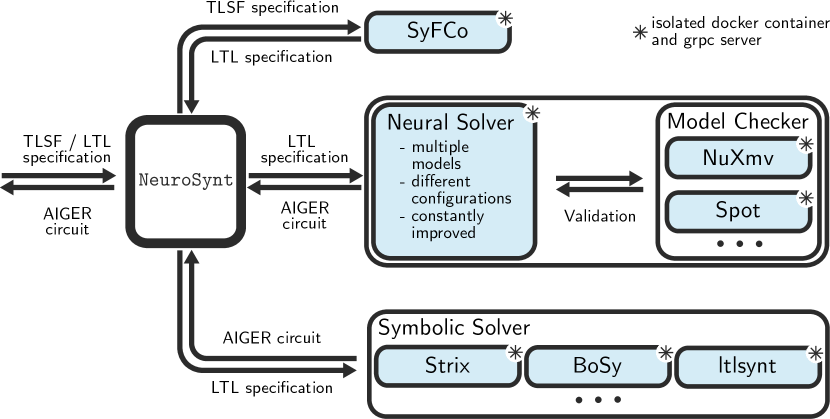
Figure 1: An overview of NeuroSynt.

We provide an overview of NeuroSynt in the following. Figure 1 shows the system design of NeuroSynt. With a single call, a sample is 1) translated from TLSF [34], the standardized input format for reactive synthesis, to LTL assumptions and guarantees. 2) Fed into the neural solver described in Section 4 with candidate solutions being verified by a model-checker. This is a feasible approach since LTL model checking is computationally significantly easier than reactive synthesis (PSPACE [61] vs. 2-EXPTIME [51]). 3) A symbolic solver is queried simultaneously with the neural solver. The final result is an implementation in the form of an AIGER [8] circuit, which is either a verified candidate circuit of the neural solver or the circuit returned by the symbolic solver. Depending on the specification’s realizability, the circuit either represents the system implementation (proving realizability) or the environment behavior (proving unrealizability).

All components, neural solver, symbolic solver, and model-checker, are isolated Docker containers. All communication channels between components are defined through a standardized API. Therefore, extending, maintaining, and updating tools are uncoupled from NeuroSynt’s implementation. Currently integrated are solvers based on the Python library ML2, including the neural solver described in Section 4, nuXmv [14], NuSMV [17], Spot [22], Strix [45], and BoSy [26]. We use SyFCo [34] to convert from TLSF to assumptions and guarantees in LTL.

3.2 Usage

Since NeuroSynt comprises multiple tools that operate in conjunction during each execution, users must specify arguments to tailor the behavior of these tools. We categorize these arguments into tool-specific and general arguments to simplify this process. General arguments are unrelated to any specific tool and are passed with the execution command in the command-line interface.

For tool-specific arguments, we use the YAML format [7] to create configuration files that encompass the neural engine arguments, the chosen tool for model checking, and symbolic synthesis tasks, along with their respective arguments. These configuration files facilitate reproducibility and provide a structured way to manage tool-specific settings. An example of a configuration file is demonstrated in Figure 11 in the Appendix.

Depending on user choice, NeuroSynt can either wait for all tools to finish/timeout and report all results or return the fastest solution. We allow the standardized input format TLSF [34] and simple assume-guarantee structured files in LTL (see Figure LABEL:app:input_format in the Appendix for an example).

NeuroSynt offers two primary execution commands: benchmark for solving a dataset of samples and synthesize for processing individual samples. For benchmark, all results are saved in a CSV file, which can be further analyzed. In all other cases, the result is printed to the command line. First, we indicate whether the specification was found to be REALIZABLE or UNREALIZABLE, after which we print the system in AIGER format [8] (see Figure 10 in the Appendix).

3.3 Implementation and Extensibility

The central design goal of NeuroSynt is to provide interfaces that are easy to implement when adding and integrating new components. We first describe the communication interfaces between components. Secondly, we detail some of the messages, and lastly, we describe the options to extend the portfolio solver.

Each solver or model-checker is isolated in a Docker container and communicates with other components through gRPC interfaces. gRPC is a high-performance open-source framework initially developed by Google for building remote procedure call (RPC) APIs. Protocol buffers (protobuf) are used as the interface definition language, ensuring programming-language-agnostic interfaces.

In Figure 2, we show the communication through gRPC APIs for the run of NeuroSynt with one specification. In the first step, each tool is initialized using setup messages, ensuring the components’ successful connection. After setup, a synthesis problem call is sent to the symbolic and neural solver in parallel. Both solvers eventually report with a synthesis solution. Before responding, the neural solver makes one or multiple calls to the model checker with candidate solutions, the specification, and the information on whether the specification is suspected to be realizable. The model checker answers a status and optionally a counterexample. The neural solver then selects one solution if multiple candidates have been generated and responds to NeuroSynt. The following details the specific protobuf messages that can be exchanged between components.

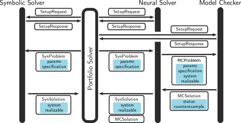
Figure 2: Communication diagram of gRPC calls for a run of NeuroSynt, calling the Symbolic Solver and the neural solver, including model-checking.

SetupRequest and SetupResponse.

As initialization, the components exchange simple messages through a JSON-like object. This message establishes the successful connection and allows the user to provide some tool- but not run-specific arguments. In the case of the neural solver, the model name and other parameters are transmitted to load the model into the memory. The component then responds with a simple success flag or error message.

SynProblem, SynSolution, and UnsoundSynSolution.

The SynProblem (request) contains an LTL Specification and a set of JSON-like parameters to configure the run- and tool-specific arguments, such as timeout or the number of threads. The LTL specification is decomposed into guarantees and assumptions, both strings in infix or prefix notation. A SynSolution contains the system as the string representation of an AIGER circuit or mealy machine, a status (realizable, unrealizable, error, timeout, nonsucess), the calculation duration, and the tool’s name. No system must be returned if error, timeout, or nonsucces were reported. The UnsoundSynSolution consists of a SynSolution and MCSolution and is returned by the neural solver. We show the protobuf definition for the SynSolution, SynProblem, and the Specification in Figure 3. Other definitions can be found in the Appendix in Figure LABEL:app:protobuf.

⬇

// An LTL Synthesis solution. Used as response message for Synthesis.

message LTLSynSolution {

// AIGER circuit. It is allowed to pass no system, e.g. if a timeout

// happened.

optional AigerCircuit circuit = 1;

// Shows, whether the specification was found to be realizable or

// unrealizable. May not be set, e.g. if a timeout happened.

optional bool realizable = 2;

// A status that includes useful information about the run.

LTLSynStatus status = 3;

// Here additional information should be supplied if the status value

// requires more details.

string detailed_status = 4;

// which tool has created the response.

Tool tool = 5;

// How long the tool took to create the result.

optional google.protobuf.Duration time = 6;

}

message LTLSynProblem {

// Defines run- and tool-specific parameters. As Map (Dict in Python).

// Typical examples are threads, timeouts etc. Can be empty.

map<string, string> parameters = 1;

// A decomposed specification (assumptions + guarantees).

DecompLTLSpecification decomp_specification = 2;

}

message DecompLTLSpecification {

// All input atomic propositions that occur in guarantees or assumptions.

repeated string inputs = 1;

// All output atomic propositions that occur in guarantees or assumptions

repeated string outputs = 2;

// A set of guarantees that make up the specifications. All inputs and

// outputs occurring in any guarantee must be part of input/output.

repeated LTLFormula guarantees = 3;

// A set of assumptions that make up the specifications. All inputs and

// outputs occurring in any guarantee must be part of input/output.

repeated LTLFormula assumptions = 4;

}

Figure 3: The protobuf definition for a SynSolution, SynProblem, and decomposed LTL specification. Slightly simplified for easier comprehension. We refer the reader to the artifact and our repository for the full definitions.

MCProblem and MCSolution.

A tool can request its candidate solutions to be model-checked by sending an MCProblem request. This message contains a set of JSON-like parameters to configure the run- and tool-specific arguments, an LTL specification (see SynProblem), and a system and status (see SynSolution). The MCSolution contains the status of the model-checking and, if violating, a counterexample in the form of an error trace and the duration of the computation. We show the relevant protobuf definitions in Figure LABEL:app:protobuf in the Appendix.

NeuroSynt can be extended in three major ways. New neural solvers, symbolic solvers, and model-checking tools can be integrated. Although not required, we recommend wrapping all components into Docker containers as it helps reproducibility, portability, and isolation, especially when run on high-performance clusters.

Neural Solver.

The neural solver sits at the core of the portfolio solver, with connections to both the model-checking component and the main portfolio solver. This component has to support receiving and responding to a SetupRequest and a SetupResponse for initialization. Furthermore, it should respond to SynProblem requests with UnsoundSynSolution. To verify candidate solutions, the neural solver should initiate communication with the model-checking component to verify candidate solutions. Therefore, it should also support sending MCProblem requests and receiving MCSolution responses. The neural solver can be independent of the ML2 library if it implements the two communication interfaces mentioned above. It can also be based on the ML2 library, where one could benefit from the existing infrastructure ML2 provides.

Model checking tools.

A model checker should respond to a SetupRequest with a SetupResponse and receive the MCProblem request, perform model checking and answer with an MCSolution.

Symbolic Solver.

New symbolic solvers can be integrated into NeuroSynt by implementing the server side of our generic protocol buffer interface for symbolic solvers. As for all components, a symbolic solver should implement a setup message (SetupRequest, SetupResponse). For a synthesis call, the symbolic solver receives a SynProblem, performs the synthesis task, and eventually responds with a SynSolution. At the time of writing, we do not require the output of synthesis tools to be model-checked. However, one can implement the interface to the model checking component to increase the trust in the output of new symbolic approaches.

4 The Neural Solver

The neural solver is at the heart of the portfolio solver and is developed jointly with NeuroSynt. We report on the methodology of the neural solver, including architecture, datasets, data generation, training, and evaluation. We clearly distinguish between previous work [56], introducing a neural approach for reactive synthesis, and improvements that are integrated into NeuroSynt, leading to the significantly increased performance on the SYNTCOMP benchmarks.

4.1 Data and Data Generation Improvement

We significantly improved the training data generation compared to previous work. While the basic algorithm is taken from [56], we scale the size of the training samples, tweak the data generation parameters to fit the larger samples, and combine multiple data generation strategies to lift previous limitations.

We aim for a dataset containing specifications (assumptions and guarantees) and circuits. Depending on the specification, the circuit is either a winning strategy for the system (realizable) or a winning strategy for the environment (unrealizable). For each sample, we use an additional token to show whether the system is realizable or unrealizable. The dataset is for supervised training, with the specification being the input and the circuit, along with the realizability token being the model’s target.

In total, we combine three datasets and generation techniques. For the first two datasets, we utilize the generation method from [56] with 1) the minor tweak of having a variable number of inputs and outputs (up to five) in the circuit instead of exactly five (denoted previous), and 2) extensions to handle a larger number of patterns, larger patterns, and patterns with more atomic propositions (denoted new). The third dataset is a data augmentation method based on the result of new (denoted augmented).

Data Generation.

We first report on the data generation algorithm for previous and new. The data generation has two major steps. In the first step, we mined LTL formula patterns that are common in research and practice. Considering formula patterns is a widespread idea, e.g., [23]. We collect patterns from $1075$ (previously $346$) benchmarks from the LTL synthesis track of SYNTCOMP 2022. We extract a list of $627$ assumption patterns and $7948$ guarantee patterns. An assumption restricts the environment, and a guarantee defines the implementation’s behavior. To fit the model requirements, we filtered out LTL formulas with more than $15$ inputs and $15$ outputs (previously $5$). Additionally, we filter out specifications with an abstract syntax tree (AST) size greater than $30$ (formerly $25$), resulting in $519$ (formerly $157$) assumption patterns and $6841$ (previously $1942$) guarantee patterns. In the second step, we constructed synthesis specifications by combining the mined patterns. For each specification, we alternate between sampling guarantees until the specification becomes unrealizable, and sampling assumptions until the specification becomes realizable. Whether we aim for a realizable or unrealizable specification, we either collect the last successfully mined specification (realizable) or the second-to-last mined specification (unrealizable). We aim for an even split between realizable and unrealizable specifications. To handle more atomic propositions while reducing patterns that do not share atomic propositions, we now favor atomic propositions present in the already constructed part of the specification with a bias of 4 when instantiating the patterns. We continue this process until we reach one of the following stopping criteria:

• the specification has the maximal number of guarantees (10),

• the specification has the maximal number of assumptions (3),

• the synthesis tool timed out (120s timeout), or

• no suitable assumption was found after 7 (formerly 5) attempts.

To ensure an even distribution of challenging instances, we filter AIGER circuits exceeding a maximum variable index of 60 and only allow a certain amount ($20\%$) of circuits with the same number of AND gates.

Data Augmentation.

We augment the dataset new as a third approach to artificially force larger properties for a share of the final dataset. For each specification in new, we combine multiple patterns into one property until we reach an AST size of $30$. Having longer properties in the training dataset leads to better generalization to even larger properties. Compared to new, the augmented dataset has an average of $3$ guarantees instead of $5.6$, with an average size of $22.9$ per guarantee instead of $12.3$.

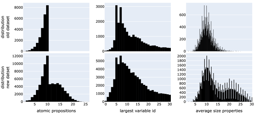
Figure 4: Previous dataset[56], compared with the new final dataset. Comparing the number of atomic propositions in a sample, the largest variable id in the AIGER circuit, and the average size of properties.

Final Dataset.

All three resulting datasets are combined into a single dataset, consisting of $600\,000$ training samples and $75\,000$ validation and test samples. Figure 4, shows the key differences in features of the new final dataset compared to the previous dataset [56]. While the previous dataset used only up to $5$ inputs and outputs in the specification, we now have up to $15$ inputs and outputs, leading to up to $25$ atomic propositions in a specification. We also have slightly more latches in the new dataset ($1.23$ instead of previously $1.16$). Note that the same version and configuration of Strix [45] was used in both approaches. The most apparent distinction to previous datasets[56] is in the size of the properties, where we clearly see the effects of the data augmentation process.

4.2 Architecture & Training

Transformer Architecture.

The core of the neural solver implemented in NeuroSynt is a Transformer neural network [62]. The vanilla Transformer architecture follows a basic encoder-decoder structure. The encoder constructs a hidden embedding $z_{i}$ for each input embedding $x_{i}$ of the input sequence $x=(x_{0},\ldots,x_{n})$ in parallel. An embedding is a mapping from plain input, for example, words or characters, to a high dimensional vector, for which learning algorithms and toolkits exist, e.g., word2vec [46]. Given the encoders output $z=(z_{0},\ldots,z_{k})$, the decoder generates a sequence of output embeddings $y=(y_{0},\ldots,y_{m})$ autoregressively. Since the transformer architecture contains no recurrence nor convolution, we apply a tree positional encoding [59].

The main idea of the Transformer is a self-attention mechanism to compute a score for each pair of input elements, representing which positions in the sequence should be considered the most when computing the hidden embeddings. For each input embedding $x_{i}$, we compute 1) a query vector $q_{i}$, 2) a key vector $k_{i}$, and 3) a value vector $v_{i}$ by multiplying $x_{i}$ with weight matrices $W_{k}$, $W_{v}$, and $W_{q}$, which are learned during the training process. The embeddings can be calculated simultaneously using matrix operations [62]. Specifically, let $Q,K,V$ be the matrices obtained by multiplying the input vector X consisting of all $x_{i}$ with the weight matrices $W_{k}$, $W_{v}$, and $W_{q}$: $\mathit{Attention}(Q,K,V)=\mathit{softmax}(\frac{QK^{T}}{\sqrt{d_{k}}})V$, with $d_{k}$ being the model’s dimension. For details, we refer the interested reader to [62]. The Transformer variation used in this paper is a so-called hierarchical Transformer [43], separating the encoder self-attention into local and global layers. Local layers embed assumptions and guarantees individually and invariant against their order. Global layers calculate the self-attention across all assumptions and all guarantees. We show an illustration in Figure 5.

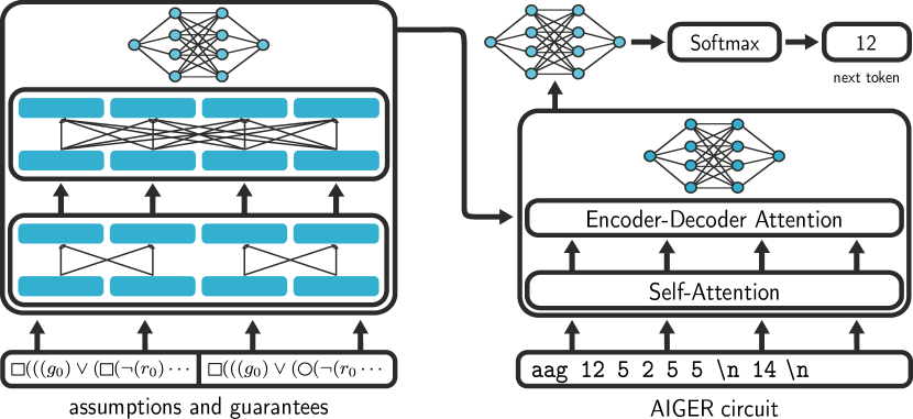
Figure 5: Schematic view of the Hierarchical Transformer, with illustrated inputs/outputs of the reactive synthesis application. The encoder shows the hierarchical self-attention with separation into local and global layers. For simplicity, we show one local and global layer and only two assumptions and guarantees with two tokens each.

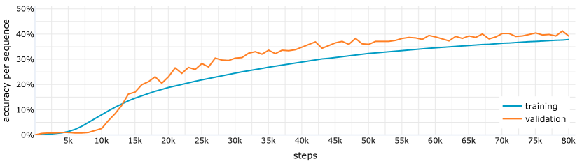
Figure 6: Accuracy per sequence during training. Measured on training and validation data.

Model Hyperparameter & Training.

We train our model on the $600\,000$ samples from our training dataset for $80\,000$ steps with early stopping and a batch size of $512$. We show a plot of the accuracy per sequence in Figure 6. We train data parallel on two Nvidia A100 40GB from a Nvidia DGX A100 system, which takes approximately $10$ hours. We use the Adam optimizer [39] with $\beta_{1}=0.9$, $\beta_{2}=0.98$ and $\epsilon=10^{-9}$. We use learning rate scheduling as proposed in [62] with $4000$ warmup-steps. Our model consists of $4$ local, $4$ global, and $8$ decoder layers, each having $4$ heads. All feed-forward networks have $1024$ nodes to which we apply a dropout of $0.2$. Our model has a total size of $14\,791\,748$ parameters. Input and output tokens have an embedding of size $256$. The maximum input and target lengths are set according to the training data with at most $12$ properties, a maximum AST size of $32$ per property for the specification, and a maximum circuit length of 128 tokens after encoding.

We show that our model significantly improved compared to previous work [56] by reimplementing and adapting the previous model to evaluate the 2022 SYNTCOMP benchmarks. With $21.8\%$, the new model improved by $13$ percentage points to $34.83\%$. We explore more details of the evaluation of the model in Section 5.1.

5 Experiments & Benchmarks

We split our experiments into two segments. In Section 5.1, we first perform generalization experiments on the integrated neural solver. The neural solver can generalize on its training distribution but also to more complex instances, longer specifications, and out-of-distribution instances, which we show using the datasets test, large, timeouts, and syntcomp.

Secondly, in Section 5.2, we evaluate the performance of the NeuroSynt framework on the SYNTCOMP 2022 benchmarks. To this end, we use NeuroSynt to compare the performance of the neural solver against multiple symbolic solvers and highlight efficiency gains and enhancements that arise from the combination of both methodologies. We show that the combined effort of neural and symbolic solvers leads to a performance gain that symbolic solvers alone could not achieve.

The evaluation is performed on a GPU cluster (1 Nvidia DGX A100 40GB, AMD EPYC 7F32 @ 1.8GHz base, 3.7GHz max, 8 cores + 8 SMT cores, 256GB RAM), on a CPU cluster (Intel Xeon E7-8867 v3 @ 2.50GHz, 64 cores + 64 HT cores, and 1536 GB RAM) and additionally did some early experiments on an Apple M1 Max (64GB memory, $10$ cores, 32 neural cores).

Similar to different configurations of symbolic solvers, we have multiple models with slightly different performances. This paper reports the results of the model that performed best on the SYNTCOMP benchmark. Whenever we consider additional models, we mention that explicitly.

5.1 Generalization

We analyze the generalization capabilities of the model in the neural solver in four ways. Firstly on our test set, secondly on samples that are significantly larger than seen during training (large), thirdly samples that are arguably more difficult than training samples, and fourthly on out-of-distribution samples (syntcomp). Here, we consider instances that are not from the same data generation algorithm out-of-distribution samples. Results on these datasets are in Table 1.

Table 1: Performance of the neural model on different datasets.

	test	large	timeouts	syntcomp- small	syntcomp- large	syntcomp- full
syntactic accuracy	$38.6\%$	$10.2\%$	-	-	-	-
semantic accuracy	$84.2\%$	$57.7\%$	$33\%$	$65.8\%$	$54.5\%$	$34.83\%$

Generalization on test and large.

On the datasets test and large, additionally to measuring correct solutions (semantic accuracy, $84.2\%$), we collect how many solutions are syntactically identical to the solution from our data generation algorithm ($38.6\%$). The large difference of $45.6$ percentage points on our test dataset indicates that the neural solver generalizes to the semantics of the synthesis problem instead of learning the particularities of the data generator.

The dataset large consists of larger samples than seen during training. Samples in large have at least $10$, on average $14.5$ properties, and the largest property in each sample has an AST of $37.9$ on average. In contrast, training samples have $5.3$ properties on average, with the largest property having an AST of $22.2$ on average.

For a more detailed analysis, we join datasets test and large and plot the share of correct solutions partitioned by the number of properties as well as the size of the largest property in each sample in Figure 7. The largest property seen during training is $30$, and the largest number of properties per specification is $12$. While we see a decrease in performance for larger samples, there is no clear drop after $12$ or $30$, respectively, which indicates generalization with the number of properties and the length of the properties. Note that results from larger sizes naturally have less significance as fewer samples per bucket exist. We refer to Figure LABEL:app:dist_large in the Appendix for the total count of samples in each displayed bucket.

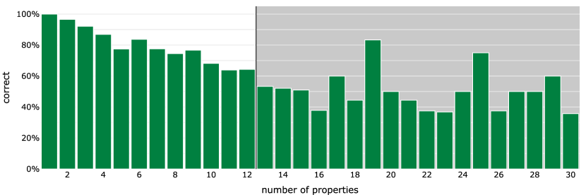
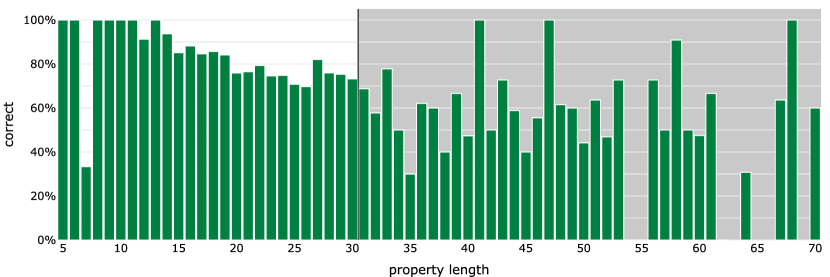
Figure 7: Share of correct solutions on the joint dataset of large and test over the number of properties in a sample and the size of the largest property in each sample. A darker background indicates sizes larger than seen during training.

Generalization on timeouts.

The dataset timeouts consists of samples on which Strix timed out after $120s$ during our data generation. Therefore, such samples can be seen as significantly harder, while not larger than samples in the training data. We achieve $33\%$ correct solutions on this dataset, showing that our model generalizes from the training data to more challenging specifications and solutions that could not have not been solved by Strix during the data generation. This experiment prognosticates the potential of combining neural methods with symbolic methods.

Generalization on out-of-distribution dataset.

While large and timeouts were generated with the same data generation approach as the training data, syntcomp-full consists of all $1075$ real-world specifications collected in the SYNTCOMP benchmark, on which the neural solver achieves $34.83\%$ accuracy (see Table 1). syntcomp-large contains all such samples that are in the size of our evaluation constraints (i.e. max $30$ properties, max AST size of $70$ per property, $54.5\%$ accuracy). syntcomp-small contains only such samples that are in the training data size (i.e., max $12$ properties, max AST size of $30$ per property, $65.8\%$ accuracy). We see a remarkable generalization to out-of-distribution samples with an accuracy of $64.8\%$ on syntcomp-small. We additionally observe generalization on specification size that we also see on the large dataset. We refer to Figure LABEL:app:share_syntcomp in the Appendix for more details.

5.2 Comparisons and Advantages of Combination

We demonstrate the advantage of NeuroSynt by comparing the neural solver to the performance of multiple symbolic solvers: Strix [45], the current state-of-the-art, BoSy [26], a bounded synthesis method, and additionally rely on the results of SYNTCOMP 2022 (ltlsynt [54], Otus [1], sdf [37]). Whenever we write SYNTCOMP in this paper, we refer to the 2022 iteration.

We initiate the evaluation by comparing the neural solver and NeuroSynt to the specified symbolic tools, illustrating the number of problems that can be solved within a specific time frame. Then we dive into details on instances that could only be solved by NeuroSynt and no other symbolic solver (novel solves), show details on the time-to-solution differences between the solvers, and lastly, look at circuit sizes of their respective solutions.

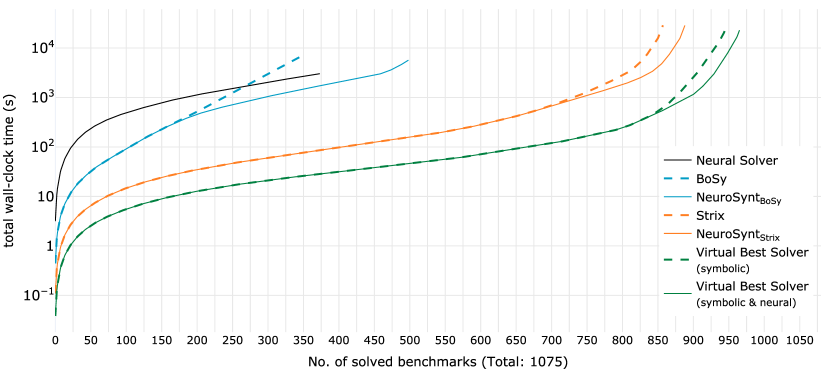
Figure 8: A cactus plot showing the number of solved samples vs. accumulated wall-clock time. Each sample per solver is a dot on the respective line. The lower and further right a line, the better the solver. We compare the neural solver, Strix and BoSy alone, NeuroSynt${}_{\text{BoSy}}$ which couples BoSy and the neural solver and NeuroSynt${}_{\text{Strix}}$ which couples the neural solver and Strix. Further, we virtually combine the results of all tools and all configurations from the SYNTCOMP to a virtual best solver and compare that with the evaluations of multiple neural models.

In Figure 8, we display the performance of the neural solver, the performance of several symbolic tools and the performance of NeuroSynt that unites the neural solver with a symbolic solver. We additionally show a Virtual Best Solver (VBS) of all SYNTCOMP 2022 results without and including the neural solver. We further report what the previously published neural reactive synthesis approach [56] would have achieved if it had been integrated into the portfolio solver. With $374$ solved instances, the neural solver alone can already solve more samples than BoSy ($347$) with $120s$ timeout on the CPU cluster. Its true advantage becomes evident when combining the neural solver with symbolic solvers. NeuroSynt${}_{\text{BoSy}}$ solves $152$ (previous: $59$) samples more than BoSy alone, which is $20.8\%$ of the samples that BoSy could not solve. Similarly, NeuroSynt${}_{\text{Strix}}$ solves $31$ (previous: $2$) samples more than Strix alone ($1h$ timeout on the CPU cluster), which is $14.2\%$ of the samples that Strix could not solve in $1h$. To show the full potential of NeuroSynt, we combined all results from the SYNTCOMP and our experiments with BoSy and Strix. All symbolic solvers combined were able to solve $945$ instances of the total of $1075$. Adding the neural solver of NeuroSynt to the virtual best solver, we solve an additional $20$ (previous: $0$) samples exclusively that no other tool tested did solve (novel solves). This is $15.4\%$ of the samples that none of the symbolic tools could solve in $1h$. No other tool in SYNTCOMP 2022 except the state-of-the-art Strix, solved more samples that no other tool could solve. We refer to the appendix LABEL:app:syntcomp-performance-exclusive for exact numbers. This signifies that even for specifications that pose computational challenges to symbolic synthesis tools, there exist patterns that a neural network can recognize and exploit post-training.

Novel Solves.

Of the $20$ novel solves, $6$ instances are parameterized versions of full arbiters with $3$ processes. This version of the full arbiter is unrealizable as the specification additionally enforces two grants to hold at the same time step (step $11$ to step $16$ respectively). These are the largest parameterizations of this problem class in the SYNTCOMP dataset. Similarly, $11$ instances are full arbiter with $3$ processes, where two grants are enforced simultaneously (step $6$ to $16$, respectively). These parameterizations are also the largest parameterizations of this problem class in the SYNTCOMP dataset. One instance is a full arbiter with $6$ processes and the requirement of two grants to hold at any time step. Finally, we have one instance of a load balancer with $6$ grants and the additional unrealizable requirement of two grants at time step $5$. This is also the largest parameterization of this problem class in the SYNTCOMP dataset. In the Appendix, Figure 13, we give an example of such samples.

Time To Solution.

For experiments with NeuroSynt, we record the wall-clock time of the neural solver, the symbolic solver, and the model checker. The neural solver (including model checking) is fastest on the GPU cluster, with $8.6s$ and a standard deviation of only $3.3s$. The time for model-checking using NuXmv is almost negligible, with $0.35s$ on average per sample. The low standard deviation highlights the advantage of the neural solver, as the time does not depend on the complexity of the specification. Strix with a timeout of $1h$ on the CPU cluster takes $33.4s$ on average, with a standard deviation of $185.3s$. We find that the neural solver can also be run on CPU-only hardware (CPU cluster) with an average of $79.4s$ and on hybrid desktop hardware such as the Apple M1 Max with an average of $17.8s$. For an extensive overview over the experiments with different timeouts, we refer the reader to the appendix LABEL:app:times.

Circuit Sizes.

We find that on instances where the neural solver and the symbolic solver both found a solution, the solution by the neural solver is often smaller than the symbolic solver’s. This holds for BoSy and Strix, but also for all other tools in SYNTCOMP (on the realizable fraction). On samples solved by Strix and the neural solver, the solutions by the neural solver have $54.9\%$ fewer latches than those by Strix. In Figure 9, we show the distribution of latches for this comparison. For more details, we refer the reader to the Appendix LABEL:app:sizes.

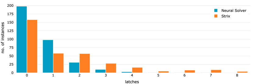
Figure 9: No. of latches per instance. On instances that the neural solver and Strix commonly solved

6 Conclusion

We introduced NeuroSynt, a neuro-symbolic portfolio solver for reactive synthesis. At the core of the portfolio solver lies an integrated neural solver that computes candidate implementations, which are automatically checked by model-checking tools. We reported on the neural solver’s methodology and training and the API framework’s implementation to isolate components. The open-source implementation of NeuroSynt provides an interface in which new neural and symbolic approaches alike can be seamlessly integrated.

Our experiments on the generalization capabilities of the Transformer show the ability to generalize to larger specifications, more difficult specifications, and out-of-distribution specifications. The relatively small size of the underlying Transformer neural network suggests that the overall performance of neural solvers can be further increased.

We evaluated the overall performance of NeuroSynt, enhancing the state-of-the-art in reactive synthesis with the integrated neural solver contributing novel solves in the SYNTCOMP 2022 benchmark. With the almost constant evaluation time of the neural solver, the portfolio solver is often faster than previous approaches. Furthermore, the integrated neural solver yields smaller implementations than state-of-the-art symbolic tools, including Strix and BoSy.

7 Data Availability Statement

NeuroSynt is published open-source on GitHub (https://github.com/reactive-systems/neurosynt). All data, models, and experiments supporting this paper’s results are publicly available. A digital artifact is available at (https://doi.org/10.5281/zenodo.10046523).

Appendix 0.A Linear-time Temporal Logic (LTL)

For a given set of atomic propositions $\mathit{AP}$, the syntax of LTL formulas over $\mathit{AP}$ is defined as:

$$\varphi,\psi\Coloneqq\operatorname{\top}~{}|~{}a~{}|~{}\neg\varphi~{}|~{}\varphi\land\psi~{}|~{}\operatorname{\leavevmode\hbox to7.41pt{\vbox to7.41pt{\text{[drawing]}}}}\varphi~{}|~{}\varphi\operatorname{\mathcal{U}}\psi\enspace,$$

where $\operatorname{\top}$ is the Boolean constant, $a\in\mathit{AP}$, $\neg$ and $\land$ are the Boolean connectives and $\operatorname{\leavevmode\hbox to7.41pt{\vbox to7.41pt{\text{[drawing]}}}}$ and $\operatorname{\mathcal{U}}$ are temporal operators. We refer to $\operatorname{\leavevmode\hbox to7.41pt{\vbox to7.41pt{\text{[drawing]}}}}$ as the next operator and to $\operatorname{\mathcal{U}}$ as the until operator. Other Boolean connectives can be derived. Further, we can derive temporal modalities such as eventually $\operatorname{\leavevmode\hbox to8.7pt{\vbox to8.7pt{\text{[drawing]}}}}\varphi\coloneqq\operatorname{\top}\operatorname{\mathcal{U}}\varphi$ and globally $\operatorname{\leavevmode\hbox to6.97pt{\vbox to6.97pt{\text{[drawing]}}}}\varphi\coloneqq\neg\operatorname{\leavevmode\hbox to8.7pt{\vbox to8.7pt{\text{[drawing]}}}}\neg\varphi$. For a given set of atomic propositions $\mathit{AP}$, the semantics of an LTL formula over $\mathit{AP}$ is defined with respect to the set of infinity words over the alphabet $2^{\mathit{AP}}$ denoted by $\left(2^{\mathit{AP}}\right)^{\omega}$. The semantics of an LTL formula $\varphi$ is defined as the language $Words(\varphi)=\{\sigma\in\left(2^{\mathit{AP}}\right)^{\omega}\mid\sigma\models\varphi\}$ where $\models$ is the smallest relation satisfying the following properties:

$$\sigma \models\operatorname{\top}$$

$$\sigma \models a \mathrm{iff}~{}a\in A_{0}$$

$$\sigma \models\neg\varphi \mathrm{iff}~{}\sigma\not\models\varphi$$

$$\sigma \models\varphi\land\psi \mathrm{iff}~{}\sigma\models\varphi~{}\mathrm{and}~{}\sigma\models\psi$$

$$\sigma \models\operatorname{\leavevmode\hbox to7.41pt{\vbox to7.41pt{\text{[drawing]}}}}\varphi \mathrm{iff}~{}\sigma[1\ldots]\models\varphi$$

$$\sigma \models\varphi\operatorname{\mathcal{U}}\psi \mathrm{iff}~{}\exists j\geq 0.~{}\sigma[j\ldots]\models\psi~{}\mathrm{and}~{}\forall 0\leq i<j.~{}\sigma[i\ldots]\models\varphi\enspace,$$

where $\sigma=A_{0}A_{1}\ldots\in(2^{\mathit{AP}})^{\omega}$ and $\sigma[i\ldots]=A_{i}A_{i+1}\ldots$ denotes the suffix of $\sigma$ starting at $i$.

A strategy $f:(2^{I})^{*}\rightarrow 2^{O}$ maps sequences of input valuations $2^{I}$ to an output valuation $2^{O}$. The behavior of a strategy $f$ is characterized by an infinite tree, called computation tree, that branches by the valuations of $I$ and whose nodes $w\in(2^{I})^{*}$ are labeled with the strategic choice $f(w)$. For an infinite word $w=w_{0}w_{1}w_{2}\ldots\in(2^{I})^{*}$, the corresponding trace is defined as $(f(\epsilon)\cup w_{0})(f(w_{0})\cup w_{1})(f(w_{1})\cup w_{2})\ldots\in(2^{I\dot{\cup}O})^{\omega}$.

Appendix 0.B Usage of NeuroSynt

We provide an example for an assume-guarantee style input file in Figure LABEL:app:input_format. It can be used as an alternative to the standardized TLSF [34] format. Figure 10 provides the output that NeuroSynt produces for this specification. In Figure 11, we give an example of the configuration file for NeuroSynt, running Strix as a symbolic solver, NuXmv as a model checker, and our neural solver.

⬇

1{

2 "semantics": "mealy",

3 "inputs": ["r_0", "r_1"],

4 "outputs": ["g_0", "g_1"],

5 "assumptions": [],

6 "guarantees": ["(G ((! (g_0)) | (! (g_1))))",

7 "(G ((r_0) -> (F (g_0))))",

8 "(G ((r_1) -> (F (g_1))))"]

9}\end{lstlisting}

10\caption{Example of the JSON input file of a simple 2-bit-arbiter}

11\label{app:input_format}

12\end{figure}

13

14

15\begin{figure}[!ht]

16 \scriptsize

17 \begin{lstlisting}[language=json]

18REALIZABLE

19aag 3 2 1 2 0

202

214

226 7

237

246

25i0 r_0

26i1 r_1

27l0 l0

28o0 g_0

29o1 g_1

Figure 10: Example of the AIGER output for a simple 2-bit arbiter

⬇

1symbolic_solver:

2 tool: strix

3 tool_args:

4 "timeout": 120

5 "--threads": 4

6 "--minimize": ""

7 "--auto": ""

8 service_args:

9 "mem_limit": "2g"

10 "start_containerized_service": True

11model_checker:

12 tool: nuxmv

13 tool_args:

14 "timeout": 10

15 service_args:

16 "mem_limit": "2g"

17 "start_containerized_service": True

18neural_solver:

19 tool: ml2solver

20 service_args:

21 "nvidia_gpus": False

22 "mem_limit": "100g"

23 "start_containerized_service": True

24 "start_service": False

25 tool_setup_args:

26 "batch_size": 1

27 "alpha": 0.5

28 "num_properties": 40

29 "length_properties": 70

30 "beam_size": 32

31 "check_setup": True

32 "model": "ht-50"

Figure 11: Example of the configuration file, running Strix as a symbolic solver, NuXmv as a model checker, and our neural solver.

Appendix 0.C Protocol Buffers

Figure LABEL:app:protobuf shows some of our protocol buffer interfaces. We omitted some messages and definitions for simplification. We refer the interested reader to the artifact.

⬇

message LTLFormula {

// Represents an LTL formula as string.

string formula = 1;

// The notation in which the formula is serialized. Infix is default.

string notation = 2;

}

message UnsoundLTLSynSolution {

LTLSynSolution synthesis_solution = 1;

// A model-checking result can optionally be included in the response.

optional LTLMCSolution model_checking_solution = 2;

// which tool has created the response.

Tool tool = 3;

// How long the tool took to create the result.

optional google.protobuf.Duration time = 4;

}

message LTLMCProblem {

// Defines run- and tool-specific parameters. As Map (Dict in Python).

// Typical examples are threads, timeouts etc. Can be empty.

map<string, string> parameters = 1;

// A decomposed specification.

DecompLTLSpecification decomp_specification = 2;

// AIGER circuit.

optional AigerCircuit circuit = 3;

// Shows whether the specification is realizable or unrealizable.

bool realizable = 4;

}

message LTLMCSolution {

// A status that includes useful information about the run.

LTLMCStatus status = 1;

// which tool has created the response.

Tool tool = 2;

// A trace, proving the violation of the specification.

optional Trace counterexample = 3;

// How long the tool took to create the result.

optional google.protobuf.Duration time = 4;

} \end{lstlisting}

\caption{Parts of the protocol buffer interfaces. Some messages and definitions are missing for simplification.}

\label{app:protobuf}

\end{figure}

\clearpage

\section{Distribution of \texttt{test}, \texttt{large}, and \texttt{syntcomp} dataset over input size}

\begin{figure}[!ht]

\includegraphics[width=\textwidth]{graphics/generalization/large_input_num_properties_count.eps}

\includegraphics[width=\textwidth]{graphics/generalization/large_input_max_prop_len_count.eps}

\caption{Distribution of the joint dataset of \texttt{large} and \texttt{test} over the number of properties in a sample and the size of the largest property in each sample.}

\label{app:dist_large}

\end{figure}

\begin{figure}[!ht]

\centering

\includegraphics[width=\textwidth]{graphics/generalization/syntcomp_input_num_properties.eps}

\includegraphics[width=\textwidth]{graphics/generalization/syntcomp_input_max_prop_len.eps}

\label{app:share_syntcomp}

\includegraphics[width=\textwidth]{graphics/generalization/syntcomp_input_num_properties_count.eps}

\includegraphics[width=\textwidth]{graphics/generalization/syntcomp_input_max_prop_len_count.eps}

\caption{Top: Share of correct solutions on the \texttt{syntcomp} datasets over the number of properties in a sample and the size of the largest property in each sample. A darker background indicates sizes larger than seen during training. Bottom: Distribution of \texttt{syntcomp} dataset over the number of properties in a sample and the size of the largest property in each sample.}

\label{app:dist_syntcomp}

\end{figure}

\clearpage

\section{Syntcomp Results}

Here, we provide detailed results on the number of solved instances (Table~\ref{app:syntcomp-performance-exclusive}), the average times per tool (Table~\ref{app:times}), and the sizes of the solutions (Table~\ref{app:sizes}).

\begin{table}[!ht]

\caption{Performance of several tools on the 2022 SYNTCOMP benchmarks. Total number of samples: 1075. Tools denoted with $\dagger$ include experiments on own hardware. Other results are solely based on the SYNTCOMP results. Exclusive solves are instances where no other listed tool provided a solution}

\setlength{\tabcolsep}{0.6em}

\label{app:syntcomp-performance-exclusive}

\begin{tabular}{@{}llll@{}}

\toprule

\multirow{2}{*}{tool} & total solved & total solved & exclusively solved \\

& best configuration & grouped configurations & grouped configurations \\ \midrule

Strix$^\dagger$ & 858 & $919$ & $116$ \\

sdf & 719 & $723$ & $17$ \\

ltlsynt & 707 & $717$ & $5$ \\

Otus & 502 & $503$ & $0$ \\

Neural Solver$^\dagger$ & 374 & $402$ & $20$ \\

BoSy$^\dagger$ & 347 & $347$ & $0$ \\ \bottomrule

\end{tabular}

\end{table}

\begin{table}[!ht]

\caption{Average times of Strix, BoSy, and the neural solver on different hardware configurations. Averaged over all SYNTCOMP instances. For the symbolic solvers, we additionally report the number of solved samples for the different hardware configurations. The Neural Solvers accuracy does not depend on the hardware configuration. Experiments on the Apple Mac Book Pro (MBP: M1 Max, 10 cores, 32 Neural Cores) are 20 randomly selected instances from SYNTCOMP. Given the low standard deviation of the neural solver that we found in other experiments, this is an accurate representation.}

\setlength{\tabcolsep}{0.6em}

\label{app:times}

\centering

\begin{tabular}{@{}llll@{}}

\toprule

Experiment & mean (s) & std (s) & solved instances\\ \midrule

Strix on CPU cluster 120s timeout & $5.1$ & $14.3$ & 821\\

Strix on GPU cluster 120s timeout & $3.7$ & $12.4$ & 833\\

Strix on CPU cluster $1h$ timeout & $33.4$ & $185.3$ & 858\\

Strix-ltl\_synth\_zlk\_bfs (SYNTCOMP) & $28.2$ & $145.7$ & 816\\

BoSy on CPU cluster 120s timeout & $19.4 $ & $28.1$ & 347\\

Neural Solver on GPU cluster & $8.6$ & $3.3 $ & \\

\;\;$\rightarrow$ thereof model-checking & $0.35$ & $0.93$ & \\

Neural Solver on CPU cluster & $79.4$ & $28$ & \\

\;\;$\rightarrow$ thereof model-checking & $0.66$ & $1.3$ & \\

Neural Solver on MBP & $17.8$ & - & \\

\;\;$\rightarrow$ thereof model-checking & $0.59$ & - & \\ \bottomrule

\end{tabular}

\end{table}

\begin{table}[!ht]

\caption{Comparison of the number of latches of different tools. Each symbolic solver is compared with the neural solver on all instances that both solvers solve correctly. Calculations on $\dagger$ marked tools are solely based on the realizable fraction of SYNTCOMP results, as SYNTCOMP only reports circuits for realizable instances.}

\setlength{\tabcolsep}{0.6em}

\label{app:sizes}

\centering

\begin{tabular}{@{}llll@{}}

\toprule

Symbolic Solver & \begin{tabular}[c]{@{}l@{}}average \\ Symbolic Solver\end{tabular} & \begin{tabular}[c]{@{}l@{}}average \\ Neural Solver\end{tabular} & \begin{tabular}[c]{@{}l@{}}Neural Solver \\ smaller by (\%)\end{tabular} \\ \midrule

Strix & 1.4 & 0.64 & 54.9 \\

BoSy & 1.11 & 0.64 & 42.3 \\

ltlsynt$^\dagger$ & 2.49 & 1.05 & 57.7 \\

Otus$^\dagger$ & 13.21 & 1.05 & 92 \\

sdf$^\dagger$ & 44.84 & 1.05 & 97.6 \\ \bottomrule

\end{tabular}

\end{table}

\section{Example Instances}

\label{app:samples}

Figure~\ref{fig:parameterized_arbiter} shows an example instance in which the neural solver found a solution, but Strix did not within the time limit.

Figure~\ref{fig:val_12} shows an example instance on which the Transformer neural network was trained on, consisting of $12$ properties.

Figure~\ref{fig:large_30} shows an example instance of the \texttt{large} data set, which was solved by the neural solver.

Figure~\ref{fig:syntcomp_40} shows an example instance from SYNTCOMP, which was solved by the neural solver (and Strix).

\begin{figure}

\centering

\scriptsize

\begin{lstlisting}[language=json]

{

"inputs": ["i0", "i1", "i2", "i3", "i4"],

"outputs": ["o0", "o1", "o2", "o3", "o4"],

"assumptions": [

"(G ((! (o0)) | (X (((! (i0)) & (! (i2))) U ((! (i0)) & (i2))))))",

"(G ((! (o2)) | (X (((! (i1)) & (! (i0))) U ((! (i1)) & (i0))))))"

],

"guarantees": [

"(G (F (o3)))",

"(G ((o0) -> (X ((i0) R (((i0) -> (o2)) & ((! (i0)) -> (o4)))))))",

"(G (((i3) & (X (i0))) -> (F ((o2) & (o0)))))",

"(G ((i0) -> (F (o3))))",

"(G (((i2) & (X (i3))) -> (X (X (X (X (X (X (X (X (X (X ((o3) & (o0))))))))))))))",

"(G ((o1) -> (X (((! (o1)) U (i3)) | (G (! (o1)))))))",

"(G (((i3) & (X (i0))) -> ((X (o1)) <-> (X (i2)))))",

"(G ((o3) -> (X (((! (o3)) U (i1)) | (G (! (o3)))))))",

"(G (((i4) & (o1)) -> (X (X (X (X (X (o4))))))))",

"(G ((X (o4)) -> (i0)))"

]

}

Figure 12: Example instance from the training set with 12 properties.

⬇

1INFO {

2 TITLE: "Full Arbiter, unrealizable variant 1"

3 DESCRIPTION: "Parameterized Arbiter, where no spurious grants are allowed"

4 SEMANTICS: Moore

5 TARGET: Mealy

6}

7{

8 "inputs": ["r_0","r_1","r_2"],

9 "outputs": ["g_0","g_1","g_2"],

10 "assumptions": [],

11 "guarantees": [

12 "(G (((g_0) & (G (! (r_0)))) -> (F (! (g_0)))))",

13 "(G (((g_0) & (X ((! (r_0)) & (! (g_0))))) -> (X ((r_0) R (! (g_0))))))",

14 "(G (((g_1) & (G (! (r_1)))) -> (F (! (g_1)))))",

15 "(G (((g_1) & (X ((! (r_1)) & (! (g_1))))) -> (X ((r_1) R (! (g_1))))))",

16 "(G (((g_2) & (G (! (r_2)))) -> (F (! (g_2)))))",

17 "(G (((g_2) & (X ((! (r_2)) & (! (g_2))))) -> (X ((r_2) R (! (g_2))))))",

18 "(G (((! (g_0)) & (! (g_1))) | (((! (g_0)) | (! (g_1))) & (! (g_2)))))",

19 "(G (((r_0) & (X (r_1))) -> (X (X (X (X (X (X (X (X (X (X (X (X (X (X (X ((g_0) & (g_1)))))))))))))))))))",

20 "(G (((r_0) & (X (r_2))) -> (X (X (X (X (X (X (X (X (X (X (X (X (X (X (X ((g_0) & (g_2)))))))))))))))))))",

21 "(G (((r_1) & (X (r_2))) -> (X (X (X (X (X (X (X (X (X (X (X (X (X (X (X ((g_1) & (g_2)))))))))))))))))))",

22 "((r_0) R (! (g_0)))",

23 "(G ((r_0) -> (F (g_0))))",

24 "((r_1) R (! (g_1)))",

25 "(G ((r_1) -> (F (g_1))))",

26 "((r_2) R (! (g_2)))",

27 "(G ((r_2) -> (F (g_2))))"

28 ]

29}

Figure 13: An instance of a parameterized arbiter without spurious grant that is solved by NeuroSynt, but not by any of the symbolic solvers.

⬇

1{

2 "inputs": ["i0","i1","i10","i11","i12","i13","i14","i2","i3","i4","i6","i7","i8","i9"],

3 "outputs": ["o0","o1","o10","o11","o12","o13","o2","o3","o4","o5","o6","o7","o8","o9"],

4 "assumptions": [

5 "G ( F ( i12 ) )",

6 "X ( G ( ( ! ( o1 ) ) | ( ( ( ! ( i13 ) ) & ( ! ( i10 ) ) ) U ( ( ! ( i13 ) ) & ( i10 ) ) ) ) )",

7 "X ( G ( ( ! ( o13 ) ) | ( ( ( ! ( i10 ) ) & ( ! ( i11 ) ) ) U ( ( ! ( i10 ) ) & ( i11 ) ) ) ) )"

8 ],

9 "guarantees": [

10 "G ( ( ( i6 ) & ( X ( i13 ) ) ) -> ( X ( X ( X ( X ( X ( X ( X ( X ( X ( ( o1 ) & ( o2 ) ) ) ) ) ) ) ) ) ) ) )",

11 "G ( ( i13 ) -> ( F ( o7 ) ) )",

12 "G ( ( o13 ) -> ( X ( ( o13 ) | ( o3 ) ) ) )",

13 "G ( ( i0 ) -> ( F ( o1 ) ) )",

14 "G ( ( i7 ) -> ( ( o2 ) <-> ( X ( o0 ) ) ) )",

15 "o3",

16 "G ( ( ( o0 ) | ( ( o13 ) & ( i11 ) ) ) -> ( X ( F ( ( ( o12 ) | ( o13 ) ) R ( i12 ) ) ) ) )",

17 "G ( ( ( ( ( ( ( ( ( ! ( i10 ) ) & ( i2 ) ) & ( ! ( i13 ) ) ) & ( ! ( i8 ) ) ) & ( ! ( i11 ) ) ) & ( ! ( i9 ) ) ) & ( ! ( i6 ) ) ) & ( i12 ) ) -> ( ( o2 ) <-> ( i0 ) ) )",

18 "G ( ( ( i2 ) & ( X ( i4 ) ) ) -> ( X ( X ( X ( X ( X ( X ( X ( ( o1 ) & ( o2 ) ) ) ) ) ) ) ) ) )",

19 "( i12 ) R ( ! ( o9 ) )",

20 "G ( ( ( ( ( ( ( ! ( i6 ) ) & ( i13 ) ) & ( ! ( i0 ) ) ) & ( i11 ) ) & ( ! ( i4 ) ) ) & ( i10 ) ) -> ( F ( ( ( ( ( ( ( ! ( o3 ) ) & ( ! ( o6 ) ) ) & ( o9 ) ) & ( ! ( o0 ) ) ) & ( o2 ) ) & ( ! ( o7 ) ) ) & ( o13 ) ) ) )",

21 "G ( ( i11 ) -> ( ( X ( ( ( ! ( o4 ) ) & ( o9 ) ) & ( ! ( o6 ) ) ) ) <-> ( i12 ) ) )",

22 "G ( ( ( ( ( ( ( o0 ) & ( ! ( o8 ) ) ) <-> ( ( ! ( o8 ) ) | ( o0 ) ) ) & ( ! ( o4 ) ) ) & ( ! ( o9 ) ) ) <-> ( ( ( ( ( o4 ) & ( ! ( o9 ) ) ) <-> ( ( o9 ) & ( ! ( o4 ) ) ) ) | ( o0 ) ) | ( o8 ) ) ) & ( ( ( ( ( ( o3 ) & ( ! ( o6 ) ) ) <-> ( ( ! ( o6 ) ) | ( o3 ) ) ) & ( ! ( o12 ) ) ) & ( ! ( o2 ) ) ) <-> ( ( ( ( ( o12 ) & ( ! ( o2 ) ) ) <-> ( ( o2 ) & ( ! ( o12 ) ) ) ) | ( o3 ) ) | ( o6 ) ) ) )",

23 "G ( ( ! ( o12 ) ) | ( ! ( o2 ) ) )",

24 "G ( ( ( ( ( ( ! ( o3 ) ) & ( o5 ) ) & ( o12 ) ) & ( ! ( o4 ) ) ) & ( G ( ( ( ( i13 ) | ( ! ( i14 ) ) ) | ( ! ( i0 ) ) ) | ( i9 ) ) ) ) -> ( F ( ( ( ( o3 ) | ( ! ( o5 ) ) ) | ( ! ( o12 ) ) ) | ( o4 ) ) ) )",

25 "o10",

26 "F ( ( i8 ) & ( ( ! ( i7 ) ) U ( ( i4 ) & ( ! ( i7 ) ) ) ) )",

27 "G ( ( i12 ) -> ( F ( o0 ) ) )",

28 "( ( ! ( i11 ) ) & ( G ( ( ( ( i11 ) & ( ! ( o8 ) ) ) -> ( X ( i11 ) ) ) & ( ( o8 ) -> ( X ( ! ( i11 ) ) ) ) ) ) ) -> ( ( ! ( o12 ) ) & ( G ( ( ( ( ( ! ( i11 ) ) & ( X ( i11 ) ) ) -> ( X ( ( ! ( o8 ) ) & ( X ( F ( o8 ) ) ) ) ) ) & ( ( ( ! ( o8 ) ) & ( X ( ! ( i11 ) ) ) ) -> ( X ( ! ( o8 ) ) ) ) ) & ( ( ! ( o12 ) ) | ( ! ( o8 ) ) ) ) ) )",

29 "G ( ( o0 ) -> ( X ( ( ( ! ( o0 ) ) U ( i3 ) ) | ( G ( ! ( o0 ) ) ) ) ) )",

30 "G ( ( ( i9 ) & ( X ( i8 ) ) ) -> ( X ( X ( X ( X ( X ( X ( X ( X ( ( o5 ) & ( o2 ) ) ) ) ) ) ) ) ) ) )",

31 "G ( F ( ( ! ( i13 ) ) | ( X ( o12 ) ) ) )",

32 "G ( ( ( ( ( ( ( ( ! ( i12 ) ) & ( i1 ) ) & ( i10 ) ) & ( ! ( i11 ) ) ) & ( i6 ) ) & ( ! ( i9 ) ) ) & ( ! ( i0 ) ) ) -> ( ( o8 ) <-> ( i3 ) ) )",

33 "G ( ( ( i13 ) & ( X ( i6 ) ) ) -> ( X ( X ( X ( X ( X ( X ( ( o11 ) & ( o8 ) ) ) ) ) ) ) ) )",

34 "G ( F ( ( ! ( i0 ) ) | ( X ( o1 ) ) ) )",

35 "G ( ( ! ( o4 ) ) | ( ! ( o9 ) ) )",

36 "G ( ( ( ! ( o7 ) ) & ( ! ( o2 ) ) ) | ( ( ( ! ( o7 ) ) | ( ! ( o2 ) ) ) & ( ! ( o5 ) ) ) )"

37 ]

38}

Figure 14: Solved example instance with $30$ properties taken from large.

⬇

1INFO {

2 TITLE: "Full Arbiter, unrealizable variant 2"

3 DESCRIPTION: "Parameterized Arbiter, where no spurious grants are allowed"

4 SEMANTICS: Mealy

5 TARGET: Mealy

6}

7

8{

9 "inputs": ["r_0","r_1","r_2","r_3","r_4","r_5"],

10 "outputs": ["g_0","g_1","g_2","g_3","g_4","g_5"],

11 "assumptions": [],

12 "guarantees": [

13 "(G (((g_0) & (G (! (r_0)))) -> (F (! (g_0)))))",

14 "(G (((g_0) & (X ((! (r_0)) & (! (g_0))))) -> (X ((r_0) R (! (g_0))))))",

15 "(G (((g_1) & (G (! (r_1)))) -> (F (! (g_1)))))",

16 "(G (((g_1) & (X ((! (r_1)) & (! (g_1))))) -> (X ((r_1) R (! (g_1))))))",

17 "(G (((g_2) & (G (! (r_2)))) -> (F (! (g_2)))))",

18 "(G (((g_2) & (X ((! (r_2)) & (! (g_2))))) -> (X ((r_2) R (! (g_2))))))",

19 "(G (((g_3) & (G (! (r_3)))) -> (F (! (g_3)))))",

20 "(G (((g_3) & (X ((! (r_3)) & (! (g_3))))) -> (X ((r_3) R (! (g_3))))))",

21 "(G (((g_4) & (G (! (r_4)))) -> (F (! (g_4)))))",

22 "(G (((g_4) & (X ((! (r_4)) & (! (g_4))))) -> (X ((r_4) R (! (g_4))))))",

23 "(G (((g_5) & (G (! (r_5)))) -> (F (! (g_5)))))",

24 "(G (((g_5) & (X ((! (r_5)) & (! (g_5))))) -> (X ((r_5) R (! (g_5))))))",

25 "(G (((((! (g_0)) & (! (g_1))) & (! (g_2))) & (((! (g_3)) & (! (g_4))) | (((! (g_3)) | (! (g_4))) & (! (g_5))))) | ((((((! (g_0)) & (! (g_1))) | (((! (g_0)) | (! (g_1))) & (! (g_2)))) & (! (g_3))) & (! (g_4))) & (! (g_5)))))",

26 "(G (((r_0) & (X (r_1))) -> (F ((g_0) & (g_1)))))",

27 "(G (((r_0) & (X (r_2))) -> (F ((g_0) & (g_2)))))",

28 "(G (((r_0) & (X (r_3))) -> (F ((g_0) & (g_3)))))",

29 "(G (((r_0) & (X (r_4))) -> (F ((g_0) & (g_4)))))",

30 "(G (((r_0) & (X (r_5))) -> (F ((g_0) & (g_5)))))",

31 "(G (((r_1) & (X (r_2))) -> (F ((g_1) & (g_2)))))",

32 "(G (((r_1) & (X (r_3))) -> (F ((g_1) & (g_3)))))",

33 "(G (((r_1) & (X (r_4))) -> (F ((g_1) & (g_4)))))",

34 "(G (((r_1) & (X (r_5))) -> (F ((g_1) & (g_5)))))",

35 "(G (((r_2) & (X (r_3))) -> (F ((g_2) & (g_3)))))",

36 "(G (((r_2) & (X (r_4))) -> (F ((g_2) & (g_4)))))",

37 "(G (((r_2) & (X (r_5))) -> (F ((g_2) & (g_5)))))",

38 "(G (((r_3) & (X (r_4))) -> (F ((g_3) & (g_4)))))",

39 "(G (((r_3) & (X (r_5))) -> (F ((g_3) & (g_5)))))",

40 "(G (((r_4) & (X (r_5))) -> (F ((g_4) & (g_5)))))",

41 "((r_0) R (! (g_0)))",

42 "(G ((r_0) -> (F (g_0))))",

43 "((r_1) R (! (g_1)))",

44 "(G ((r_1) -> (F (g_1))))",

45 "((r_2) R (! (g_2)))",

46 "(G ((r_2) -> (F (g_2))))",

47 "((r_3) R (! (g_3)))",

48 "(G ((r_3) -> (F (g_3))))",

49 "((r_4) R (! (g_4)))",

50 "(G ((r_4) -> (F (g_4))))",

51 "((r_5) R (! (g_5)))",

52 "(G ((r_5) -> (F (g_5))))"

53 ]

54}

Figure 15: Solved example instance from SYNTCOMP with $40$ properties.

References

- [1] Abraham, R.: Symbolic LTL reactive synthesis. Master’s thesis, University of Twente, Enschede (Jul 2021)
- [2] Alet, F., Lopez-Contreras, J., Koppel, J., Nye, M., Solar-Lezama, A., Lozano-Perez, T., Kaelbling, L., Tenenbaum, J.: A large-scale benchmark for few-shot program induction and synthesis. In: International Conference on Machine Learning. pp. 175–186. PMLR (2021)
- [3] Alon, Y., David, C.: Using graph neural networks for program termination. In: Proceedings of the 30th ACM Joint European Software Engineering Conference and Symposium on the Foundations of Software Engineering. pp. 910–921. ESEC/FSE 2022, Association for Computing Machinery, New York, NY, USA (Nov 2022). https://doi.org/10.1145/3540250.3549095
- [4] Balunovic, M., Bielik, P., Vechev, M.T.: Learning to solve SMT formulas. In: Bengio, S., Wallach, H.M., Larochelle, H., Grauman, K., Cesa-Bianchi, N., Garnett, R. (eds.) Advances in Neural Information Processing Systems 31: Annual Conference on Neural Information Processing Systems 2018, NeurIPS 2018, December 3-8, 2018, Montréal, Canada. pp. 10338–10349 (2018)
- [5] Bansal, K., Loos, S.M., Rabe, M.N., Szegedy, C., Wilcox, S.: HOList: An Environment for Machine Learning of Higher-Order Theorem Proving. In: Proceedings of the 36th International Conference on Machine Learning. pp. 454–463. PMLR (May 2019). https://doi.org/10.48550/arXiv.1904.03241
- [6] Bansal, K., Szegedy, C., Rabe, M.N., Loos, S.M., Toman, V.: Learning to reason in large theories without imitation (Jun 2020). https://doi.org/10.48550/arXiv.1905.10501
- [7] Ben-Kiki, O., Evans, C., döt Net, I.: YAML Ain’t Markup Language (YAML™) revision 1.2.2. Tech. rep. (Oct 2021)
- [8] Biere, A.: The AIGER And-Inverter Graph (AIG) format version 20071012. Tech. Rep. 07/1, Institute for Formal Models and Verification, Johannes Kepler University, Altenbergerstr. 69, 4040 Linz, Austria (October 2007, 2007)
- [9] Biere, A., Heljanko, K., Wieringa, S.: AIGER 1.9 and beyond. Tech. Rep. 11/2, Institute for Formal Models and Verification, Johannes Kepler University, Altenbergerstr. 69, 4040 Linz, Austria (July 2011, 2011)
- [10] Büchi, J.R., Landweber, L.H.: Solving sequential conditions by finite-state strategies. Transactions of the American Mathematical Society 138, 295–311 (1969). https://doi.org/10.2307/1994916
- [11] Cadilhac, M., Pérez, G.A.: Acacia-bonsai: a modern implementation of downset-based LTL realizability. In: Sankaranarayanan, S., Sharygina, N. (eds.) Tools and Algorithms for the Construction and Analysis of Systems - 29th International Conference, TACAS 2023, Paris, France, April 22-27, 2023, Proceedings, Part II. Lecture Notes in Computer Science, vol. 13994, pp. 192–207. Springer (2023). https://doi.org/10.1007/978-3-031-30820-8_14
- [12] Calude, C.S., Jain, S., Khoussainov, B., Li, W., Stephan, F.: Deciding parity games in quasipolynomial time. In: Hatami, H., McKenzie, P., King, V. (eds.) Proceedings of the 49th Annual ACM SIGACT Symposium on Theory of Computing, STOC 2017, Montreal, QC, Canada, June 19-23, 2017. pp. 252–263. ACM (2017). https://doi.org/10.1145/3055399.3055409
- [13] Cameron, C., Chen, R., Hartford, J., Leyton-Brown, K.: Predicting propositional satisfiability via end-to-end learning. In: Proceedings of the AAAI Conference on Artificial Intelligence. vol. 34, pp. 3324–3331 (2020)
- [14] Cavada, R., Cimatti, A., Dorigatti, M., Griggio, A., Mariotti, A., Micheli, A., Mover, S., Roveri, M., Tonetta, S.: The nuXmv symbolic model checker. In: Biere, A., Bloem, R. (eds.) Computer Aided Verification - 26th International Conference, CAV 2014, Vienna, Austria, July 18-22, 2014. Proceedings. Lecture Notes in Computer Science, vol. 8559, pp. 334–342. Springer (2014). https://doi.org/10.1007/978-3-319-08867-9_22
- [15] Church, A.: Logic, arithmetic, and automata (1962)
- [16] Church, A.: Application of recursive arithmetic to the problem of circuit synthesis. In: Summaries of the Summer Institute of Symbolic Logic. vol. 1, pp. 3–50. Cornell University, Ithaca, NY (1957)
- [17] Cimatti, A., Clarke, E., Giunchiglia, E., Giunchiglia, F., Pistore, M., Roveri, M., Sebastiani, R., Tacchella, A.: NuSMV 2: an OpenSource tool for symbolic model checking. In: Brinksma, E., Larsen, K.G. (eds.) Computer Aided Verification. pp. 359–364. Lecture Notes in Computer Science, Springer, Berlin, Heidelberg (2002). https://doi.org/10.1007/3-540-45657-0_29
- [18] Clymo, J., Manukian, H., Fijalkow, N., Gascón, A., Paige, B.: Data generation for neural programming by example. In: Proceedings of the Twenty Third International Conference on Artificial Intelligence and Statistics. pp. 3450–3459. PMLR (2020)
- [19] Cosler, M., Hahn, C., Mendoza, D., Schmitt, F., Trippel, C.: nl2spec: interactively translating unstructured natural language to temporal logics with large language models. In: Enea, C., Lal, A. (eds.) Computer Aided Verification - 35th International Conference, CAV 2023, Paris, France, July 17-22, 2023, Proceedings, Part II. Lecture Notes in Computer Science, vol. 13965, pp. 383–396. Springer (2023). https://doi.org/10.1007/978-3-031-37703-7_18
- [20] Cosler, M., Schmitt, F., Hahn, C., Finkbeiner, B.: Iterative circuit repair against formal specifications. In: The Eleventh International Conference on Learning Representations, ICLR 2023, Kigali, Rwanda, May 1-5, 2023 (2023)
- [21] Drori, I., Zhang, S., Shuttleworth, R., Tang, L., Lu, A., Ke, E., Liu, K., Chen, L., Tran, S., Cheng, N., Wang, R., Singh, N., Patti, T.L., Lynch, J., Shporer, A., Verma, N., Wu, E., Strang, G.: A neural network solves, explains, and generates university math problems by program synthesis and few-shot learning at human level. Proceedings of the National Academy of Sciences 119(32), e2123433119 (Aug 2022). https://doi.org/10.1073/pnas.2123433119
- [22] Duret-Lutz, A., Renault, E., Colange, M., Renkin, F., Aisse, A.G., Schlehuber-Caissier, P., Medioni, T., Martin, A., Dubois, J., Gillard, C., Lauko, H.: From Spot 2.0 to Spot 2.10: what’s new? In: Shoham, S., Vizel, Y. (eds.) Computer Aided Verification - 34th International Conference, CAV 2022, Haifa, Israel, August 7-10, 2022, Proceedings, Part II. Lecture Notes in Computer Science, vol. 13372, pp. 174–187. Springer (2022). https://doi.org/10.1007/978-3-031-13188-2_9
- [23] Dwyer, M.B., Avrunin, G.S., Corbett, J.C.: Patterns in property specifications for finite-state verification. In: Proceedings of the 21st international conference on Software engineering. pp. 411–420. ICSE ’99, Association for Computing Machinery, New York, NY, USA (May 1999). https://doi.org/10.1145/302405.302672
- [24] Ehlers, R.: Unbeast: symbolic bounded synthesis. In: Abdulla, P.A., Leino, K.R.M. (eds.) Tools and Algorithms for the Construction and Analysis of Systems - 17th International Conference, TACAS 2011, Saarbrücken, Germany, March 26-April 3, 2011. Proceedings. Lecture Notes in Computer Science, vol. 6605, pp. 272–275. Springer (2011). https://doi.org/10.1007/978-3-642-19835-9_25
- [25] Ellis, K., Wong, L., Nye, M., Sablé-Meyer, M., Cary, L., Anaya Pozo, L., Hewitt, L., Solar-Lezama, A., Tenenbaum, J.B.: DreamCoder: growing generalizable, interpretable knowledge with wake–sleep Bayesian program learning. Philosophical Transactions of the Royal Society A: Mathematical, Physical and Engineering Sciences 381(2251), 20220050 (Jun 2023). https://doi.org/10.1098/rsta.2022.0050
- [26] Faymonville, P., Finkbeiner, B., Tentrup, L.: BoSy: an experimentation framework for bounded synthesis. In: Majumdar, R., Kuncak, V. (eds.) Computer Aided Verification - 29th International Conference, CAV 2017, Heidelberg, Germany, July 24-28, 2017, Proceedings, Part II. Lecture Notes in Computer Science, vol. 10427, pp. 325–332. Springer (2017). https://doi.org/10.1007/978-3-319-63390-9_17
- [27] Fijalkow, N., Lagarde, G., Matricon, T., Ellis, K., Ohlmann, P., Potta, A.N.: Scaling neural program synthesis with distribution-based search. In: Proceedings of the AAAI Conference on Artificial Intelligence. vol. 36, pp. 6623–6630 (Jun 2022). https://doi.org/10.1609/aaai.v36i6.20616
- [28] Finkbeiner, B., Hahn, C., Lukert, P., Stenger, M., Tentrup, L.: Synthesis from hyperproperties. Acta Informatica 57(1-2), 137–163 (2020). https://doi.org/10.1007/s00236-019-00358-2
- [29] Finkbeiner, B., Klein, F.: Bounded cycle synthesis. In: Chaudhuri, S., Farzan, A. (eds.) Computer Aided Verification - 28th International Conference, CAV 2016, Toronto, ON, Canada, July 17-23, 2016, Proceedings, Part I. Lecture Notes in Computer Science, vol. 9779, pp. 118–135. Springer (2016). https://doi.org/10.1007/978-3-319-41528-4_7
- [30] First, E., Rabe, M.N., Ringer, T., Brun, Y.: Baldur: Whole-Proof Generation and Repair with Large Language Models (Mar 2023). https://doi.org/10.48550/arXiv.2303.04910
- [31] Giacobbe, M., Kroening, D., Parsert, J.: Neural termination analysis. In: Roychoudhury, A., Cadar, C., Kim, M. (eds.) Proceedings of the 30th ACM Joint European Software Engineering Conference and Symposium on the Foundations of Software Engineering, ESEC/FSE 2022, Singapore, Singapore, November 14-18, 2022. pp. 633–645. ACM, Singapore Singapore (Nov 2022). https://doi.org/10.1145/3540250.3549120
- [32] Hahn, C., Schmitt, F., Kreber, J.U., Rabe, M.N., Finkbeiner, B.: Teaching temporal logics to neural networks. In: 9th International Conference on Learning Representations, ICLR 2021, Virtual Event, Austria, May 3-7, 2021 (2021)
- [33] Huang, D., Dhariwal, P., Song, D., Sutskever, I.: GamePad: a learning environment for theorem proving. In: 7th International Conference on Learning Representations, ICLR 2019, New Orleans, LA, USA, May 6-9, 2019 (2019)
- [34] Jacobs, S., Klein, F., Schirmer, S.: A high-level LTL synthesis format: TLSF v1.1. In: Piskac, R., Dimitrova, R. (eds.) Proceedings Fifth Workshop on Synthesis, SYNT@CAV 2016, Toronto, Canada, July 17-18, 2016. EPTCS, vol. 229, pp. 112–132 (2016). https://doi.org/10.4204/EPTCS.229.10
- [35] Jacobs, S., Perez, G.A., Abraham, R., Bruyere, V., Cadilhac, M., Colange, M., Delfosse, C., van Dijk, T., Duret-Lutz, A., Faymonville, P., Finkbeiner, B., Khalimov, A., Klein, F., Luttenberger, M., Meyer, K., Michaud, T., Pommellet, A., Renkin, F., Schlehuber-Caissier, P., Sakr, M., Sickert, S., Staquet, G., Tamines, C., Tentrup, L., Walker, A.: The reactive synthesis competition (SYNTCOMP): 2018-2021 (Jun 2022). https://doi.org/10.48550/arXiv.2206.00251
- [36] Jiang, A.Q., Welleck, S., Zhou, J.P., Lacroix, T., Liu, J., Li, W., Jamnik, M., Lample, G., Wu, Y.: Draft, Sketch, and Prove: Guiding Formal Theorem Provers with Informal Proofs. In: The Eleventh International Conference on Learning Representations, ICLR 2023, Kigali, Rwanda, May 1-5, 2023 (2023)
- [37] Khalimov, A.: Game-based bounded synthesis via BDDs
- [38] Khalimov, A., Jacobs, S., Bloem, R.: PARTY parameterized synthesis of token rings. In: Sharygina, N., Veith, H. (eds.) Computer Aided Verification - 25th International Conference, CAV 2013, Saint Petersburg, Russia, July 13-19, 2013. Proceedings. Lecture Notes in Computer Science, vol. 8044, pp. 928–933. Springer (2013). https://doi.org/10.1007/978-3-642-39799-8_66
- [39] Kingma, D.P., Ba, J.: Adam: a method for stochastic optimization. In: Bengio, Y., LeCun, Y. (eds.) 3rd International Conference on Learning Representations, ICLR 2015, San Diego, CA, USA, May 7-9, 2015, Conference Track Proceedings (2015). https://doi.org/10.48550/arXiv.1412.6980
- [40] Kreber, J.U., Hahn, C.: Generating symbolic reasoning problems with transformer GANs (May 2023). https://doi.org/10.48550/arXiv.2110.10054
- [41] Křetínský, J., Meggendorfer, T., Prokop, M., Rieder, S.: Guessing winning policies in LTL synthesis by semantic learning. In: Enea, C., Lal, A. (eds.) Computer Aided Verification. pp. 390–414. Lecture Notes in Computer Science, Springer Nature Switzerland, Cham (2023). https://doi.org/10.1007/978-3-031-37706-8_20
- [42] Lample, G., Charton, F.: Deep learning for symbolic mathematics. In: 8th International Conference on Learning Representations, ICLR 2020, Addis Ababa, Ethiopia, April 26-30, 2020 (2020)
- [43] Li, W., Yu, L., Wu, Y., Paulson, L.C.: IsarStep: a benchmark for high-level mathematical reasoning. In: 9th International Conference on Learning Representations, ICLR 2021, Virtual Event, Austria, May 3-7, 2021 (2021)
- [44] Loos, S.M., Irving, G., Szegedy, C., Kaliszyk, C.: Deep network guided proof search. In: Eiter, T., Sands, D. (eds.) LPAR-21, 21st International Conference on Logic for Programming, Artificial Intelligence and Reasoning, Maun, Botswana, May 7-12, 2017. EPiC Series in Computing, vol. 46, pp. 85–105. EasyChair (2017). https://doi.org/10.29007/8mwc
- [45] Meyer, P.J., Sickert, S., Luttenberger, M.: Strix: explicit reactive synthesis strikes back! In: Chockler, H., Weissenbacher, G. (eds.) Computer Aided Verification. pp. 578–586. Lecture Notes in Computer Science, Springer International Publishing, Cham (2018). https://doi.org/10.1007/978-3-319-96145-3_31
- [46] Mikolov, T., Chen, K., Corrado, G., Dean, J.: Efficient estimation of word representations in vector space. In: Bengio, Y., LeCun, Y. (eds.) 1st International Conference on Learning Representations, ICLR 2013, Scottsdale, Arizona, USA, May 2-4, 2013, Workshop Track Proceedings (2013)
- [47] Paliwal, A., Loos, S.M., Rabe, M.N., Bansal, K., Szegedy, C.: Graph representations for higher-order logic and theorem proving. In: The Thirty-Fourth AAAI Conference on Artificial Intelligence, AAAI 2020, New York, NY, USA, February 7-12, 2020. pp. 2967–2974. AAAI Press (2020). https://doi.org/10.1609/aaai.v34i03.5689
- [48] Pei, K., Bieber, D., Shi, K., Sutton, C., Yin, P.: Can large language models reason about program invariants? In: International Conference on Machine Learning. pp. 27496–27520. PMLR (2023)
- [49] Piterman, N., Pnueli, A., Sa’ar, Y.: Synthesis of reactive(1) designs. In: Emerson, E.A., Namjoshi, K.S. (eds.) Verification, Model Checking, and Abstract Interpretation, 7th International Conference, VMCAI 2006, Charleston, SC, USA, January 8-10, 2006, Proceedings. Lecture Notes in Computer Science, vol. 3855, pp. 364–380. Springer (2006). https://doi.org/10.1007/11609773_24
- [50] Pnueli, A.: The temporal logic of programs. In: 18th Annual Symposium on Foundations of Computer Science, Providence, Rhode Island, USA, 31 October - 1 November 1977. pp. 46–57 (Oct 1977). https://doi.org/10.1109/SFCS.1977.32
- [51] Pnueli, A., Rosner, R.: On the synthesis of a reactive module. In: Conference Record of the Sixteenth Annual ACM Symposium on Principles of Programming Languages, Austin, Texas, USA, January 11-13, 1989. pp. 179–190. ACM Press (1989). https://doi.org/10.1145/75277.75293
- [52] Pnueli, A., Rosner, R.: Distributed reactive systems are hard to synthesize. In: 31st Annual Symposium on Foundations of Computer Science, St. Louis, Missouri, USA, October 22-24, 1990, Volume II. pp. 746–757. IEEE Computer Society (1990). https://doi.org/10.1109/FSCS.1990.89597
- [53] Rabin, M.: Automata on infinite objects and church’s problem. CBMS Regional Conference Series in Mathematics, vol. 13. American Mathematical Society, Providence, Rhode Island (1972). https://doi.org/10.1090/cbms/013
- [54] Renkin, F., Schlehuber, P., Duret-Lutz, A., Pommellet, A.: Improvements to ltlsynt (2022). https://doi.org/10.48550/arXiv.2201.05376
- [55] Ryan, G., Wong, J., Yao, J., Gu, R., Jana, S.: CLN2INV: Learning Loop Invariants with Continuous Logic Networks. In: International Conference on Learning Representations (Sep 2019)
- [56] Schmitt, F., Hahn, C., Rabe, M.N., Finkbeiner, B.: Neural circuit synthesis from specification patterns. In: Advances in Neural Information Processing Systems. vol. 34, pp. 15408–15420. Curran Associates, Inc. (2021)
- [57] Selsam, D., Bjørner, N.S.: Guiding high-performance SAT solvers with unsat-core predictions. In: Janota, M., Lynce, I. (eds.) Theory and Applications of Satisfiability Testing - SAT 2019 - 22nd International Conference, SAT 2019, Lisbon, Portugal, July 9-12, 2019, Proceedings. Lecture Notes in Computer Science, vol. 11628, pp. 336–353. Springer (2019). https://doi.org/10.1007/978-3-030-24258-9_24
- [58] Selsam, D., Lamm, M., Bünz, B., Liang, P., de Moura, L., Dill, D.L.: Learning a SAT solver from single-bit supervision. In: 7th International Conference on Learning Representations, ICLR 2019, New Orleans, LA, USA, May 6-9, 2019 (2019)
- [59] Shiv, V.L., Quirk, C.: Novel positional encodings to enable tree-based transformers. In: Wallach, H.M., Larochelle, H., Beygelzimer, A., d’Alché-Buc, F., Fox, E.B., Garnett, R. (eds.) Advances in Neural Information Processing Systems 32. pp. 12058–12068. Vancouver, BC, Canada (Dec 2019)
- [60] Si, X., Dai, H., Raghothaman, M., Naik, M., Song, L.: Learning loop invariants for program verification. In: Advances in Neural Information Processing Systems. vol. 31 (2018)
- [61] Sistla, A.P., Clarke, E.M.: The complexity of propositional linear temporal logics. Journal of the ACM (JACM) 32(3), 733–749 (1985). https://doi.org/10.1145/3828.3837
- [62] Vaswani, A., Shazeer, N., Parmar, N., Uszkoreit, J., Jones, L., Gomez, A.N., Kaiser, L., Polosukhin, I.: Attention is all you need. In: Guyon, I., von Luxburg, U., Bengio, S., Wallach, H.M., Fergus, R., Vishwanathan, S.V.N., Garnett, R. (eds.) Advances in Neural Information Processing Systems 30. pp. 5998–6008. Long Beach, CA, USA (Dec 2017)
- [63] Wu, Y., Jiang, A.Q., Li, W., Rabe, M., Staats, C., Jamnik, M., Szegedy, C.: Autoformalization with large language models. Advances in Neural Information Processing Systems 35, 32353–32368 (2022)