Out-of-Distribution Detection & Applications With Ablated Learned Temperature Energy

Abstract

As deep neural networks become adopted in high-stakes domains, it is crucial to be able to identify when inference inputs are Out-of-Distribution (OOD) so that users can be alerted of likely drops in performance and calibration (Ovadia et al., 2019) despite high confidence (Nguyen et al., 2015). Among many others, existing methods use the following two scores to do so without training on any apriori OOD examples: a learned temperature (Hsu et al., 2020) and an energy score (Liu et al., 2020). In this paper we introduce Ablated Learned Temperature Energy (or "AbeT" for short), a method which combines these prior methods in novel ways with effective modifications. Due to these contributions, AbeT lowers the False Positive Rate at 95% True Positive Rate (FPR@95) by $35.39\%$ in classification (averaged across all ID and OOD datasets measured) compared to state of the art without training networks in multiple stages or requiring hyperparameters or test-time backward passes. We additionally provide empirical insights as to how our model learns to distinguish between In-Distribution (ID) and OOD samples while only being explicitly trained on ID samples via exposure to misclassified ID examples at training time. Lastly, we show the efficacy of our method in identifying predicted bounding boxes and pixels corresponding to OOD objects in object detection and semantic segmentation, respectively - with an AUROC increase of $5.15\%$ in object detection and both a decrease in FPR@95 of $41.48\%$ and an increase in AUPRC of $34.20\%$ on average in semantic segmentation compared to previous state of the art.

1 Introduction

In recent years, machine learning models have shown impressive performance on fixed distributions (Lin et al., 2017; Ren et al., 2015; Girshick, 2015; Liu et al., 2016; Redmon et al., 2016; Dai et al., 2016; Radford et al., 2021; Feichtenhofer, 2020; Devlin et al., 2018; Dosovitskiy et al., 2020). However, the distribution from which examples are drawn at inference time is not always stationary or overlapping with the training distribution. In these cases where inference examples are far from the training set, not only does model performance drop, all known uncertainty estimates also become uncalibrated (Ovadia et al., 2019). Without OOD detection, users can be completely unaware of these drops in performance and calibration, and often can be fooled into false trust in model predictions due to high confidence on OOD inputs (Nguyen et al., 2015). Thus, identifying the presence of examples which are far from the training set is of utmost importance to AI safety and reliability.

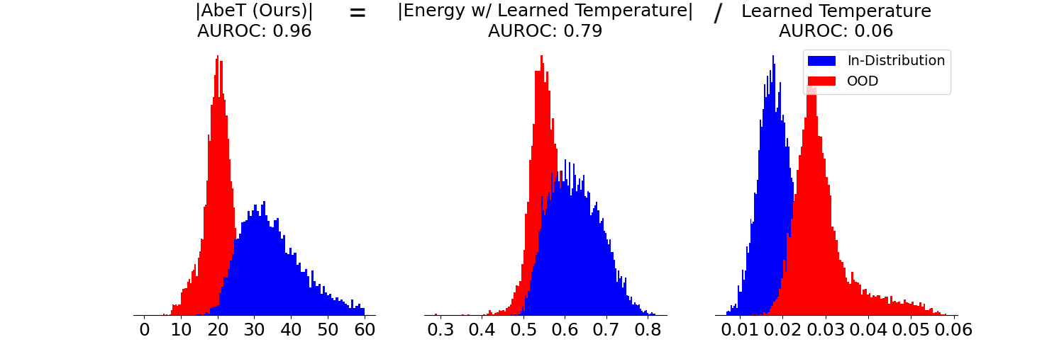
Figure 1: Histograms showing the separability between OOD scores on OOD inputs (red) and ID inputs (blue) for different methods. The goal is to make these red and blue distributions as separable as possible, with OOD scores on OOD inputs (red) close to 0 and OOD scores on ID inputs (blue) of high-magnitude (away from 0). (Center) Our first contribution is replacing the Scalar Temperature in the Energy Score (Liu et al., 2020) with a Learned Temperature (Hsu et al., 2020). This infusion leads to Equation 7, with the Learned Temperature showing up in the Exponential Divisor Temperature (overlined in Equation 7) and Forefront Temperature Constant (underlined in Equation 7) forms. (Right) The Forefront Temperature Constant contradicts the desired property of scores being close to 0 for OOD points (red) and of high magnitude for ID points (blue). (Left) Therefore, our second contribution is to ablate this Forefront Temperature Constant, leading to our final Ablated Learned Temperature Energy (AbeT) score. This ablation increases the separability of the OOD scores vs. ID scores, as can be seen visually and numerically (in terms of AUROC) comparing the center and left plots - where the only difference is this ablation of the Forefront Temperature Constant. Higher AUROC means more separability.

Aimed at OOD detection, existing methods have explored (among many other methods) modifying models via a learned temperature which is dynamic depending on input (Hsu et al., 2020) and an inference-time post-processing energy score which measures the log of the exponential sum of logits on a given input, scaled by a scalar temperature (Liu et al., 2020). We combine these methods and provide improvements. Due to these contributions, we demonstrate the efficacy of AbeT over existing OOD methods. We establish state of the art performance in classification, object detection, and semantic segmentation on a suite of common OOD benchmarks spanning a variety of scales and resolutions. We also perform extensive visual and empirical investigations to understand our algorithm. Our key results and contributions are as follows:

• We combine the learned temperature (Hsu et al., 2020) and post-processing energy score (Liu et al., 2020) by simply using the learned temperature in the calculation of the energy score.

• We resolve a contradiction in the energy score (Liu et al., 2020) by ablating one of the learned temperature terms. We deem this "Ablated Learned Temperature Energy" (or "AbeT" for short) and it serves as our ultimate OOD score.

• We provide visual and empirical evidence to provide intuition as to why our method is able to achieve superior OOD detection performance without being exposed to explicit OOD inputs at training time via OOD samples resembling misclassified ID samples.

• We show the efficacy of using AbeT in identifying predicted bounding boxes and pixels corresponding to OOD objects in object detection and semantic segmentation, respectively.

2 Background

Let $X:\Omega\to\mathcal{X}\subset\mathbb{R}^{D}$ be the input (random) variable and let $Y:\Omega\to\{1,2,...,C-1,C\}\subset\mathbb{N}$ (where $c$ is the number of output classes) be the response (random) variable. Typically $X$ has some information about $Y$ and we’d like to make inferences about $Y$ given $X$ using a learned model $\hat{f}:\mathbb{R}^{D}\to\mathbb{R}^{C}$. In practice, a learner only has access to a limited amount of training examples in this data-set on which to train $\hat{f}$

$$D^{train}_{in}=\{(x_{i},y_{i})\}_{i=1}^{N}$$ (1)

which are examples drawn from $(X,Y)$ (or a subset thereof).

2.1 Problem Statement

Let $D_{in}^{test}$ and $D_{out}^{test}$ represent the ID and OOD datasets, respectively defined similarity to the dataset definition in Equation 1 that are unseen at training time. In our evaluations, we define $D^{test}_{out}$ as any dataset that has non-overlapping output classes with the output classes of $D^{train}_{in}$, as is standard in OOD detection evaluations (Huang et al., 2021; Hsu et al., 2020; Liu et al., 2020; Djurisic et al., 2022; Sun et al., 2021; Hendrycks & Gimpel, 2016; Liang et al., 2017; Sun et al., 2022; Katz-Samuels et al., 2022). The goal of Out-of-Distribution Detection is to define a score $G:X\rightarrow\{0,1\}$ such that

$$G(x;f,\theta)=\begin{cases}0,&\mathrm{if\hskip 2.84526pt}x\in D_{in}^{test}\\ 1,&\mathrm{if\hskip 2.84526pt}x\in D_{out}^{test}\par\end{cases}$$ (2)

2.2 Standard Classification Model Optimization

In OOD detection, $\hat{f}$ serves a dual purpose: its outputs are directly optimized to classify among outputs $\{1,2,...,C-1,C\}$ and functions of the network are used as inputs to $G$. Though we use $\hat{f}$ for both purposes, our aim is for AbeT to neither have OOD data at training time nor significantly modify training to account for the ability to detect OOD data. Therefore, we train our classification models in a standard way: to minimize a risk function

$$\mathcal{R}=\sum_{i=1}^{N}\mathcal{L}(\hat{f}(x_{i};\theta),y_{i})$$

where $\mathcal{L}$ is a loss function and $(x_{i},y_{i})\in D^{train}_{in}$. In deep learning classification settings, the Cross-Entropy loss function is normally used for training: $\mathcal{L}_{CE}(\hat{f}(x_{i};\theta),y_{i})=-\log\hat{f}_{y_{i}}(x_{i};\theta)$, where $\hat{f}_{y_{i}}(x_{i};\theta)$ is the output of the model $\hat{f}$ corresponding to the ground truth class $y_{i}$ on input $x_{i}$. Our method is theoretically compatible with other loss functions, but we did not explicitly test our method in conjunction with any loss function other than Cross-Entropy.

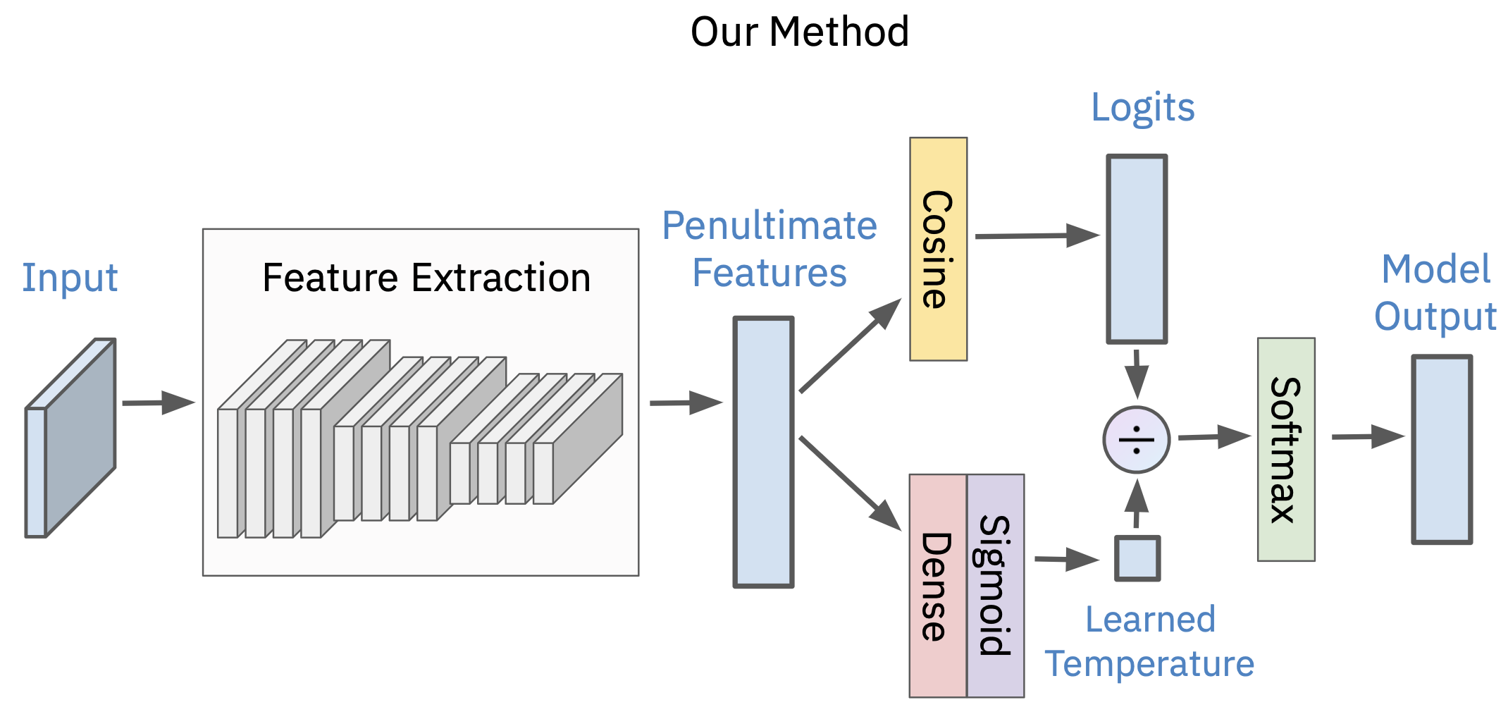
Figure 2: Architecture of the forward pass of a classification network with a learned temperature.

2.3 Model Output

To estimate $\hat{f}_{y_{i}}(x_{i};\theta)$, models typically use logit functions per class which calculate the activation of class $c$ on input $x_{i}$ as $L_{c}(x_{i};\theta)=\hat{g}_{c}(x_{i};\theta)$. $\hat{g}_{c}$ will be defined below in Section 2.3.3. Often employed to increase calibration, Temperature Scaling (Guo et al., 2017) geometrically decreases the logit function $L$ by a single scalar $T$. That is, $\hat{f}$ has a logit function that employs a scalar temperature $L_{c}(x_{i};\theta,T_{\mathrm{scalar}})=\hat{g}_{c}(x_{i};\theta)/T_{\mathrm{scalar}}$. Introduced in Hsu et al. (2020), a learned temperature $T_{\mathrm{learned}}:\mathcal{X}\rightarrow(0,1)$ is a temperature that depends on input $x_{i}$. That is, $\hat{f}$ has a logit function that employs a learned temperature

$$L_{c}(x_{i};\theta,T_{\mathrm{learned}})=\hat{g}_{c}(x_{i};\theta)/T_{\mathrm{learned}}(x_{i})$$ (3)

The softmax of this tempered logit serves as the final model prediction

$$\hat{f}_{y_{i}}(x_{i};\theta)=\dfrac{\exp\left(\hat{g}_{y_{i}}(x_{i};\theta)/T_{\mathrm{learned}}(x_{i})\right)}{\sum_{c=1}^{C}\exp\left(\hat{g}_{c}(x_{i};\theta)/T_{\mathrm{learned}}(x_{i})\right)}$$ (4)

which is fed into the cross entropy loss during training. In this formulation, the model has two mechanisms by which it can reduce loss: increasing confidence (via high $\hat{g}_{y_{i}}(x_{i};\theta)$ or low $T_{\mathrm{learned}}(x_{i})$) when correct or decreasing confidence via high $T_{\mathrm{learned}}(x_{i})$ when incorrect.

We provide a visual architecture of our forward pass in Figure 2.

2.3.1 Learned Temperature Details

For all AbeT models, our learned temperature function is architecturally identical to that in Hsu et al. (2020): a single fully connected layer which takes inputs from the penultimate layer and outputs a single scalar per input, passes these scalars through a Batch Normalization layer, then activates these scalars via a sigmoid which normalizes them to $(0,1)$. The learned temperature is automatically trained via the gradients induced by the back-propagation of the network’s optimization since the learned temperature modifies the logits used in the forwards pass of the model. In this way, it is updated like any other layer which affects the forwards pass of the network, and thus requires no tuning, training, or datasets other than the cross-entropy-based optimization using the training dataset. The only requirement to train the learned temperature is this one-line architectural change prior to training. For information on limitations due to this requirement, please see Appendix Section A.1.

2.3.2 Memory and Timing Costs Due To Learned Temperature

The time and memory costs due to the operations of the learned temperature are relatively light-weight in comparison to that of the forward pass of the model without the learned temperature. For example, with Places365 as the inference OOD dataset, the forward pass of our method took $0.94$ seconds while the forward pass of the baseline model (without the learned temperature) took $0.92$ seconds, a difference of less than $3\%$. As an example of insignificant additional space costs necessary for the use of our method, the baseline ResNet20 (without the learned temperature) used in our CIFAR experiments has $275572$ parameters, and our learned temperature adds a mere $64$ parameters to this. This increases memory usage by less than $1\%$.

2.3.3 Logit Function

Let $w$ and $b$ represent the weights and biases of the final layer of a classification network (mapping penultimate space to output space) respectively and $f^{p}(x_{i})$ represent the penultimate representation of the network on input $x_{i}$. Normally, deep classification networks use the inner product of the $w$ and $x_{i}$ (plus the bias term) as the logit function

$$\hat{g}_{c}(x_{i};\theta)=w_{c}^{T}f^{p}(x_{i})+b_{c}$$ (5)

However, Hsu et al. (2020) found that a logit function based on the cosine similarity between $w$ and $f^{p}(x_{i})$ was more effective when training logit functions that serve this dual-purpose of classifying among outputs $\{1,2,...,C-1,C\}$ and as an input to $G$

$$\hat{g}_{c}(x_{i};\theta)=\dfrac{w_{c}^{T}f^{p}(x_{i})}{||w_{c}^{T}||||f^{p}(x_{i})||}$$ (6)

We therefore use this cosine-similarity score as our logit function $\hat{g}$.

3 Our Approach

The following post-processing energy score was previously used for OOD detection in Liu et al. (2020): $\mathrm{E}(x_{i};L,T_{\mathrm{scalar}},\theta)=-T_{\mathrm{scalar}}\log\sum_{c=1}^{C}e^{L_{c}(x_{i};\theta,T_{\mathrm{scalar}})}$ . This energy score was intended to be highly negative on ID input and close to $0$ on OOD inputs via high logits on ID inputs and low logits on OOD inputs.

Our first contribution is replacing the scalar temperature with a learned one:

$$\mathrm{E}(x_{i};L,T_{\mathrm{learned}},\theta)=-\underbrace{T_{\mathrm{learned}}(x_{i})}_{\text{Forefront Temperature Constant}}\log\sum_{c=1}^{C}e^{L_{c}(x_{i};\theta,\overbrace{T_{\mathrm{learned}})}^{\text{Exponential Divisor Temperature}}}$$ (7)

By introducing this learned temperature, there become two ways to control the OOD score: by modifying the logits and by modifying the learned temperature. We note that there are two different operations that the learned temperature performs in terms of modifying the energy score. We deem these two operations the "Forefront Temperature Constant" and the "Exponential Divisor Temperature", which are underlined and overlined, respectively, in Equation 7. Our second contribution is noting that only the Exponential Divisor Temperature contributes to the OOD score being in adherence with this property of highly negative on ID inputs and close to $0$ on OOD inputs, while Forefront Temperature Constant counteracts that property - we therefore ablate this Forefront Temperature Constant. To see this, we note that the learned temperature is trained to be higher on inputs on which the classifier is uncertain - such as OOD and misclassified ID inputs - in order to deflate the softmax confidence on those inputs (i.e. increase softmax uncertainty); and the learned temperature is trained to be lower on inputs on which the classifier is certain - such as correctly classified ID inputs - in order to inflate the softmax confidence on those inputs (i.e. increase softmax certainty). Thus, the temperature term being high on OOD inputs and low on ID inputs leads to the energy score being closer to $0$ on OOD inputs and more highly negative on ID inputs when used in the Exponential Divisor Term, as desired. However, the temperature term being high on OOD inputs and low on ID inputs leads to the energy score being more highly negative on OOD inputs and closer to $0$ on ID inputs when being used in the Forefront Temperature Constant, which is the opposite of what we would like. We therefore (as previously mentioned) simply ablate the Forefront Temperature Constant, leading to the following Ablated Temperature Energy score:

$$\mathrm{{AbeT}}(x_{i};L,T_{\mathrm{learned}},\theta)=-\log\sum_{c=1}^{C}e^{L_{c}(x_{i};\theta,T_{\mathrm{learned}})}$$

We visualize the effects of this ablation in Figure 1, using Places365 (Zhou et al., 2018) as the OOD dataset, CIFAR-100 (Krizhevsky, 2009) as the ID dataset, and a ResNet-20 (He et al., 2016a) trained with learned temperature and a cosine logit head as the model.

Finally, we define $\hat{G}$ as an estimator for $G$ in Equation 2:

$$G(x;f,\theta)=\begin{cases}0,&\mathrm{if\hskip 2.84526pt}|\mathrm{{AbeT}}(x_{i};L,T_{\mathrm{learned}},\theta)|\geq\gamma\\ 1,&\mathrm{if\hskip 2.84526pt}|\mathrm{{AbeT}}(x_{i};L,T_{\mathrm{learned}},\theta)|<\gamma\par\end{cases}$$ (8)

where $\gamma$ is a hyperparameter chosen depending on user-preference in terms of balance between Precision and Recall.

4 Classification Experiments

In the following sections, we evaluate our OOD score and compare with recent methods on a variety of OOD benchmarks in classification. We describe our experimental setup in Section 4.1. In Section 4.2, we show the superior performance of AbeT over existing approaches.

4.1 Classification Experimental Setup

4.1.1 Classification Datasets

$D_{in}^{test}$	CIFAR-10		CIFAR-100		ImageNet-1k
Method	FPR@95 $\downarrow$	AUROC $\uparrow$	FPR@95 $\downarrow$	AUROC $\uparrow$	FPR@95 $\downarrow$	AUROC $\uparrow$
MSP	60.52 $\pm$ 15.2	89.59 $\pm$ 3.8	82.72 $\pm$ 11.0	71.92 $\pm$ 7.6	63.91 $\pm$ 8.2	79.29 $\pm$ 5.7
ODIN	39.12 $\pm$ 24.8	92.46 $\pm$ 4.6	73.36 $\pm$ 31.8	75.30 $\pm$ 13.5	72.99 $\pm$ 7.9	82.56 $\pm$ 5.5
Mahalanobis	37.16 $\pm$ 35.6	86.84 $\pm$ 17.2	72.41 $\pm$ 22.7	77.57 $\pm$ 18.5	81.69 $\pm$ 19.9	62.02 $\pm$ 11.0
Gradient Norm	28.39 $\pm$ 24.9	93.12 $\pm$ 6.4	56.10 $\pm$ 38.8	81.72 $\pm$ 13.8	54.70 $\pm$ 7.5	86.31 $\pm$ 4.2
DNN	49.03 $\pm$ 11.3	83.45 $\pm$ 5.0	66.65 $\pm$ 13.8	78.60 $\pm$ 5.8	61.90 $\pm$ 6.5	82.99 $\pm$ 3.9
GODIN	26.88 $\pm$ 10.1	94.27 $\pm$ 2.0	47.06 $\pm$ 7.6	90.74 $\pm$ 2.3	52.79 $\pm$ 5.7	83.97 $\pm$ 4.7
Energy	39.70 $\pm$ 24.4	92.59 $\pm$ 4.4	70.57 $\pm$ 32.5	78.01 $\pm$ 12.5	71.03 $\pm$ 7.5	82.74 $\pm$ 5.4
Energy + ReAct	39.67 $\pm$ 15.3	93.04 $\pm$ 2.7	62.82 $\pm$ 17.7	86.30 $\pm$ 6.8	31.43*	92.95*
Energy + DICE	20.83 $\pm$ 1.5	95.24 $\pm$ 0.2	49.72 $\pm$ 1.6	87.23 $\pm$ 0.7	34.75*	90.77*
Energy + ASH	20.05 $\pm$ 21.4	95.45 $\pm$ 5.1	37.61 $\pm$ 34.3	89.67 $\pm$ 12.3	16.78 $\pm$ 13.7	96.59 $\pm$ 2.2
AbeT	12.51 $\pm$ 2.0	97.81 $\pm$ 0.4	31.19 $\pm$ 12.3	94.05 $\pm$ 1.8	40.00 $\pm$ 11.4	91.80 $\pm$ 3.0
AbeT + ReAct	12.22 $\pm$ 1.9	97.82 $\pm$ 0.4	26.21 $\pm$ 7.6	94.19 $\pm$ 2.2	38.19 $\pm$ 11.6	92.21 $\pm$ 3.1
AbeT + DICE	11.61 $\pm$ 2.2	97.90 $\pm$ 0.4	31.33 $\pm$ 13.0	94.36 $\pm$ 2.21	30.70 $\pm$ 15.1	93.20 $\pm$ 3.8
AbeT + ASH	10.99 $\pm$ 5.7	97.90 $\pm$ 0.9	30.64 $\pm$ 12.7	94.46 $\pm$ 2.2	3.71 $\pm$ 3.5	99.00 $\pm$ 0.8

* Results where a ResNet-50 is used as in their corresponding papers instead of ResNet-101 as in our experiments. This is due to our inability to reproduce their results with ResNet-101

Table 1: Comparison with other competitive OOD detection methods in classification. OOD detection results on a suite of standard datasets compared against competitive methods which are trained with ID data only and require only one stage of training. All results are averaged across 4 OOD datasets, with the standard deviations calculated across these same 4 OOD datasets. $\uparrow$ means higher is better and $\downarrow$ means lower is better.

We follow standard practices in OOD evaluations (Huang et al., 2021; Hsu et al., 2020; Liu et al., 2020; Djurisic et al., 2022; Sun et al., 2021; Hendrycks & Gimpel, 2016; Liang et al., 2017; Sun et al., 2022; Katz-Samuels et al., 2022) in terms of metrics, ID datasets, and OOD datasets. For evaluation metrics, we use AUROC and FPR@95. We measure performance at varying number of ID classes via CIFAR-10 (Krizhevsky, 2009), CIFAR-100 (Krizhevsky, 2009), and ImageNet-1k (Huang & Li, 2021). For our CIFAR experiments, we use 4 OOD datasets standard in OOD detection: Textures (Cimpoi et al., 2014), SVHN (Netzer et al., 2011), LSUN (Crop) (Yu et al., 2015), and Places365 (Zhou et al., 2018). For our ImageNet-1k experiments we also evaluate on four standard OOD test datasets, but subset these datasets to classes that are non-overlapping with respect to ImageNet-1k as is common practice (Huang et al., 2021; Sun et al., 2022, 2021; Sun & Li, 2021): iNaturalist (Van Horn et al., 2018), SUN (Xiao et al., 2010), Places365 (Zhou et al., 2018), and Textures (Cimpoi et al., 2014). See Appendix D.1.1 for details about these datasets.

4.1.2 Classification Models and Hyperparameters

For all experiments with CIFAR-10 and CIFAR-100 as ID data, we use a ResNet-20 (He et al., 2016a). For all experiments with ImageNet-1k as ID data, we use a ResNetv2-101 (He et al., 2016b). We present additional experiments where we retain top OOD performance with ImageNet-1k as the ID data using an alternative architecture, DenseNet-121 (Huang et al., 2017), in Appendix Section B.3. All models are trained from scratch. For more experimental details, see Appendix Section D.2.1.

4.1.3 Previous Classification Approaches

We compare against previous methods with similar constraints, training settings, and testing settings. We note that we do not compare against other methods that are trained on OOD data (Ming et al., 2022; Katz-Samuels et al., 2022; Hendrycks et al., 2018) or methods that require multiple stages of training (Khalid et al., 2022). Principally, we compare against Maximum Softmax Probability (Hendrycks & Gimpel, 2016), ODIN (Liang et al., 2017), GODIN (Hsu et al., 2020), Mahalanobis (Lee et al., 2018), Energy Score (Liu et al., 2020), Gradient Norm (Huang et al., 2021), ReAct (Sun et al., 2021), DICE (Sun & Li, 2021), Deep Nearest Neighbors (DNN) (Sun et al., 2022), and ASH (Djurisic et al., 2022). For more details about these competitive methods, see Appendix Section E.

4.2 Performance On Standard OOD in Classification Suite

In Table 1, we compare against the aforementioned methods outlined in Section 4.1.3. All results are averaged across the four previously mentioned OOD test datasets per ID dataset outlined in Section 4.1.1, with the standard deviations calculated across these same 4 OOD datasets. All OOD methods keep accuracy within $1\%$ of their respective baseline methods without any modifications to account for OOD. Results from MSP (Hendrycks & Gimpel, 2016), ODIN (Liang et al., 2017), Energy (Lee et al., 2018), and Gradient Norm (Huang et al., 2021) are taken directly from Huang et al. (2021), as their models, datasets, and hyperparameters are identical to ours. We provide detailed results for each OOD test dataset in Appendix Section B.

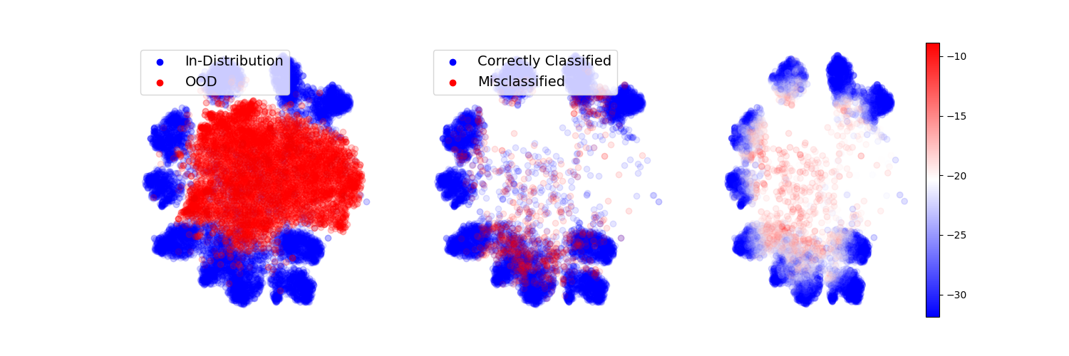
Figure 3: (Left) Scatter plot of OOD LSUN examples (red) and ID test CIFAR-10 examples (blue). (Center) ID test CIFAR-10 examples correctly classified (blue) and incorrectly classified (red). (Right) ID test CIFAR-10 examples colored by their AbeT score. Red is estimated to be more OOD. The learned temperature increasing on misclassified points leads OOD scores inflating towards 0 on misclassified points. The presence of a comparatively higher proportion of points in the center which are misclassified therefore leads to the relationship that our OOD scores inflate towards 0 as distance to the center decreases, which can be visually seen on ID points in the right plot. In combination with OOD points lying in the center (as can be seen on the left plot), this means that our OOD scores are close to 0 on OOD points - thus providing intuition (but not proof) as to why our method is able to achieve superior OOD detection performance.

We note that our method achieves an average reduction in FPR@95 of $53.46\%$ on CIFAR-10, $33.72\%$ on CIFAR-100, and $20.61\%$ on ImageNet. We additionally note that not only is the mean performance of our method superior in all settings, but the standard deviation of our performance across OOD datasets is relatively low in nearly all cases, meaning our method is consistently performant.

We additionally present a study of our Forefront Temperature Constant ablation in Appendix Section B.1 and show that this singular ablation contribution leads to a reduction in FPR@95 of $28.76\%$, $59.00\%$, and $24.81\%$ with CIFAR-10, CIFAR-100, and ImageNet as the ID datasets respectively (averaged across their 4 respective OOD datasets) compared to AbeT without the Forefront Temperature Constant ablation (i.e. if AbeT were to be defined as Equation 7).

In Appendix Section B.4, we present Gradient Input Perturbation (Liang et al., 2017) in conjunction with our method and show that it harmed our method.

We also present experiments in Appendix Section B.2 where we replace the Cosine Logit Head (defined in Equation 6) with the standard Inner Product Head (defined in Equation 5) and show that the Cosine Logit Head significantly improves the performance of our method, reaffirming the finding of Hsu et al. (2020) that the Cosine Logit Head is preferable over the Inner Product Head in OOD Detection.

5 Understanding AbeT

In Section 5, we provide intuition-building evidence to suggest that the superior OOD performance of AbeT despite not being exposed to explicit OOD samples at training time is due to exposure to misclassified ID examples during training. Towards building intuition we provide visual evidence in Figure 3 based on TSNE-reduced (Van der Maaten & Hinton, 2008) embeddings to support the following two hypotheses:

1. Our method learns a representation function such that the proportion of ID points near OOD points which are misclassified is higher than the proportion of misclassified ID points overall

2. Our OOD scores are comparatively higher (closer to 0) on misclassified ID examples

These combined hypotheses suggest that the OOD score behavior learned on misclassified points applies to OOD points more than ID points overall. OOD scores are therefore close to 0 on OOD points due to the OOD points learning this inflation of OOD scores (towards 0) of the (sparse) misclassified points near them, while this inflation of OOD scores doesn’t apply as much to ID points overall - as desired. This is learned without ever being exposed to OOD points at training time.

In Appendix Section C.1, we present empirical evidence to support these two hypothesis which does not utilize dimensionality reduction.

6 Applications in Semantic Segmentation & Object Detection

Figure 4: Qualitative comparison of OOD scores for semantic segmentation. The top row and bottom row contain examples from the datasets RoadAnomaly (Lis et al., 2019) and LostAndFound (Pinggera et al., 2016), respectively. Pixels corresponding to OOD objects are highlighted in red in each image in the leftmost column, which are cropped to regions where we have ID/OOD labels. Scores for each example (row) and technique (column) are thresholded at their respective 95% True Positive Rate and then normalized $[0,1]$ in the red channel, with void pixels (which have no ID/OOD label) set to 0. Bright red pixels represent high OOD scores, which should cover the same region as the pixels which correspond to OOD objects in the leftmost column. We invert the scores of Standardized Max Logit, Max Logit, and MSP to allow these methods to highlight OOD pixels in red.

6.1 Semantic Segmentation

In Table 2, we compare against competitive OOD Detection methods in semantic segmentation that predict which pixels correspond to object classes not found in the training set (i.e. which pixels correspond to OOD objects). We report evaluation metrics over FPR@95, AUPRC, and AUROC and compare against methodologies which follow similar training, inference, and dataset paradigms. For our experiments with AbeT, we replace the Inner Product per-pixel in the final convolutional layer with a Cosine Logit head per-pixel and a learned temperature layer per-pixel. Further details about model training can be found in Appendix Section D.2.2. For datasets, we use Mapillary (Neuhold et al., 2017) and Cityscapes (Cordts et al., 2016) as the ID datasets and LostAndFound (Pinggera et al., 2016) and RoadAnomaly (Lis et al., 2019) as the OOD datasets. Details about these OOD Datasets can be found in Appendix Section D.1.2. All results from Standardized Max Logit (SML) (Jung et al., 2021), Max Logit (ML) (Hendrycks et al., 2022), and PEBAL (Tian et al., 2022) are taken from Tian et al. (2022). Mahalanobis (MHLBS) (Lee et al., 2018) results for LostAndFound and RoadAnomaly are taken from (Chan et al., 2021) and (Tian et al., 2022), respectively. Additionally, we compare to entropy (Chan et al., 2021) and Max Softmax Probability (MSP) (Hendrycks & Gimpel, 2016). Similar to classification, we do not compare with methods which fine-tune or train on OOD (or OOD proxy data like COCO (Lin et al., 2014b)) (Chan et al., 2021; Tian et al., 2022) or with methods which significantly change training (Mukhoti & Gal, 2018). We additionally do not compare with methods which involve multiple stages of OOD score refinement by leveraging the geometric location of the scores (Jung et al., 2021; Chan et al., 2021), as these refinement processes could be performed on top of any given OOD score in semantic segmentation. We do not compare to these methods as our approach is task-agnostic, does not require any OOD data or refinement of the OOD scores, and requires minimal changes to the training and inference of existing deep learning models.

Notably, our method reduces FPR@95 by $78.02\%$ on LostAndFound and increases AUPRC by $63.96\%$ on RoadAnomaly compared to competitive methods.

We also present visualizations of pixel-wise OOD predictions for our method and methods against which we compare on a selection of images from OOD datasets in Figure 4.

$D_{in}^{test}$		LostAndFound			RoadAnomaly
Method	ID Cityscapes mIOU	FPR@95 $\downarrow$	AUPRC $\uparrow$	AUROC $\uparrow$	FPR@95 $\downarrow$	AUPRC $\uparrow$	AUROC $\uparrow$
Entropy	81.39	35.47	46.01	93.42	65.26	16.89	68.24
MSP	81.39	31.80	27.49	91.98	56.28	15.24	65.96
SML	81.39	44.48	25.89	88.05	70.70	17.52	75.16
ML	81.39	15.56	65.45	94.52	70.48	18.98	72.78
MHLBS	81.39	27	48	-	81.09	14.37	62.85
AbeT	80.56	3.42	68.35	99.09	53.5	31.12	81.55
PEBAL	80	0.81	78.29	99.76	44.58	45.10	87.63

Table 2: Comparison with other competitive OOD detection methods in semantic segmentation. OOD detection results on a suite of standard datasets compared against competitive methods which are trained with ID data only, only require one stage of training, and which do not perform any inference-time OOD score refinement based on geometric location. We present PEBAL (Tian et al., 2022) which trains on OOD data to provide context as to current performance of methods which do have access to OOD samples at training time, rather than presenting it as a competitive method against which we directly compare. $\uparrow$ means higher is better and $\downarrow$ means lower is better.

Method	ID AP $\uparrow$	FPR@95 $\downarrow$	AUROC $\uparrow$	AUPRC $\uparrow$
Basline	40.2	91.47	60.65	88.69
VOS (Du et al., 2022)	40.5	88.67	60.46	88.49
AbeT (Ours)	41.2	88.81	65.34	91.76

Table 3: Comparison with other competitive OOD detection methods in object detection. ID model performance and OOD performance of baseline model, state of the art OOD object detection method Virtual Outlier Synthesis (Du et al., 2022), and our method, all of which do not have access to OOD at training time. $\uparrow$ means higher is better and $\downarrow$ means lower is better.

6.2 Object Detection

For evaluating AbeT on object detection tasks we use the PASCAL VOC dataset (Everingham et al., 2010) as the ID dataset and COCO (Lin et al., 2014a) as the OOD dataset. The learned temperature and Cosine Logit Head are directly attached to a FasterRCNN classification head’s penultimate layer as described in the above sections. Further training details can be found in Appendix Section D.2.3. Our method is compared with a baseline FasterRCNN model and a FasterRCNN model using the state of the art VOS method proposed by Du et al. (2022). For evaluation metrics we use the ID AP and OOD metrics FPR@95, AUROC, and AUPRC. ID AP is calculate as standard object detection algorithm across all ID classes. OOD metrics are calculated by treating ID box predictions as positives and OOD box predictions as negatives. These evaluation metrics are calculated without thresholding detections based on any of the ID or OOD scores. Results can be viewed in Table 3.

We note that our method shows improved performance on ID AP (via the learned temperature decreaseing confidence on OOD-induced false positives), AUROC, and AUPRC with comparable performance on FPR@95. Our method provides the added benefit of being a single, lightweight modification to detectors’ classification heads as opposed to significant changes to training with additional Virtual Outlier Synthesis, loss functions, and hyperparameters as in Du et al. (2022).

7 Conclusion

Inferences on examples far from a model’s training set tend to be significantly less performant than inferences on examples close to its training set. Moreover, even if a model is calibrated on a holdout ID dataset, the confidence scores corresponding to these inferences on OOD examples cannot be trusted to be reflective of performance because confidence scores can become greatly misaligned with performance when predicting on examples far from the model’s training set (Ovadia et al., 2019). In other words, not only does performance drop on OOD examples - users are often completely unaware of these performance drops. Therefore, detecting OOD examples in order to alert users of likely miscalibration and performance drops is one of the biggest hurdles to overcome in AI safety and reliability. Towards detecting OOD examples, we have introduced AbeT which mixes a learned temperature (Hsu et al., 2020) and an energy score (Liu et al., 2020) in a novel way with an ablation. We have established the superiority of AbeT in detecting OOD examples in classification, detection, and segmentation. We have additionally provided visual and empirical evidence as to how our method is able to achieve superior performance.

Appendix

Appendix A Our Method

A.1 Limitations

In our experimentation, our method only worked well if this learned temperature was learned in conjunction with the rest of the layers from scratch. Therefore, this requirement of an architectural change means our method has a limitation in that it can only be used by those who can train a new model from scratch with our one-line architectural change, which is not a requirement of OOD methods which can be used on pre-trained models post-hoc.

Appendix B Detailed Performance

For detailed performance of all OOD methods (baseline methods and AbeT) on each OOD dataset separately, please see Table 4 for AUROC results on CIFAR, Table 5 for AUROC results on ImageNet, Table 6 for FPR@95 results on CIFAR, and Table 7 for FPR@95 results on ImageNet.

				$D_{out}^{test}$
$D_{in}^{test}$	Method	Textures	SVHN	LSUN	Places365	Average
	MSP (Hendrycks & Gimpel, 2016)	87.62	89.86	94.87	85.99	89.59
	ODIN (Liang et al., 2017)	89.99	89.63	99.39	90.81	92.46
	Energy (Liu et al., 2020)	88.79	91.97	99.03	90.55	92.59
	Mahalanobis (Lee et al., 2018)	92.31	95.99	97.9	61.15	86.84
CIFAR-10	Gradient Norm (Huang et al., 2021)	90.76	96.66	99.87	85.2	93.12
	DNN (Sun et al., 2022)	77.53	85.43	81.59	89.26	83.45
	GODIN (Hsu et al., 2020)	95.11	92.58	92.57	96.83	94.28
	ReAct (Sun et al., 2021)	91.46	93.03	92.81	91.92	92.32
	DICE (Sun & Li, 2021)	91.40	93.24	92.77	91.86	92.32
	AbeT (Ours)	97.17	97.93	98.09	98.04	97.81
	MSP (Hendrycks & Gimpel, 2016)	64.02	72.56	82.06	69.05	71.92
	ODIN (Liang et al., 2017)	66.35	66.85	95.09	72.90	75.30
	Energy (Liu et al., 2020)	66.74	76.42	95.90	72.98	78.01
	Mahalanobis (Lee et al., 2018)	87.48	81.71	90.74	50.35	77.57
CIFAR-100	Gradient Norm (Huang et al., 2021)	81.83	79.35	99.69	65.99	81.72
	DNN (Sun et al., 2022)	72.16	76.94	79.15	86.15	78.60
	GODIN (Hsu et al., 2020)	91.14	88.21	90.05	93.56	90.74
	ReAct (Sun et al., 2021)	81.11	87.46	85.46	83.72	84.44
	DICE (Sun & Li, 2021)	83.57	91.25	87.49	85.92	87.06
	AbeT (Ours)	95.49	91.55	93.65	96.44	94.05

Table 4: AUROC comparison with other competitive OOD detection in classification methods on CIFAR. Detection results on a suite of standard datasets compared against competitive methods which are trained with ID data only and require only one stage of training. Higher AUROC is better.

				$D_{out}^{test}$
$D_{in}^{test}$	Method	Textures	iNaturalist	SUN	Places365	Average
	MSP (Hendrycks & Gimpel, 2016)	74.45	87.59	78.34	76.76	79.29
	ODIN (Liang et al., 2017)	76.30	89.36	83.92	80.67	82.56
	Energy (Liu et al., 2020)	75.79	88.48	85.32	81.37	82.74
	Mahalanobis (Lee et al., 2018)	72.10	46.33	65.20	64.46	62.02
ImageNet-1k	Gradient Norm (Huang et al., 2021)	81.07	90.33	89.03	84.82	86.31
	DNN (Sun et al., 2022)	78.89	81.61	88.17	83.27	82.99
	GODIN (Hsu et al., 2020)	77.67	86.41	88.51	83.29	83.97
	ReAct (Sun et al., 2021)	80.33	86.95	79.35	78.70	81.33
	DICE (Sun & Li, 2021)	83.07	91.59	86.61	84.67	86.49
	AbeT (Ours)	92.03	95.82	90.95	88.39	91.80

Table 5: AUROC comparison with other competitive OOD detection in classification methods on ImageNet-1k. Detection results on a suite of standard datasets compared against competitive methods which are trained with ID data only and require only one stage of training. Higher AUROC is better.

				$D_{out}^{test}$
$D_{in}^{test}$	Method	Textures	SVHN	LSUN	Places365	Average
	MSP (Hendrycks & Gimpel, 2016)	68.32	66.09	37.73	70.05	60.53
	ODIN (Liang et al., 2017)	52.78	55.52	2.32	45.86	39.12
	Energy (Liu et al., 2020)	58.67	49.80	3.86	46.48	39.70
	Mahalanobis (Lee et al., 2018)	28.83	20.91	9.66	89.24	37.16
CIFAR-10	Gradient Norm (Huang et al., 2021)	37.71	17.76	0.23	57.85	28.39
	DNN (Sun et al., 2022)	52.30	56.20	55.40	32.20	49.03
	GODIN (Hsu et al., 2020)	20.30	32.10	38.40	16.70	26.88
	ReAct (Sun et al., 2021)	52.52	48.09	48.90	561.75	50.32
	DICE (Sun & Li, 2021)	52.25	46.99	48.34	52.14	49.93
	AbeT (Ours)	15.31	12.37	10.61	11.74	12.51
	MSP (Hendrycks & Gimpel, 2016)	90.64	86.33	66.33	87.57	82.72
	ODIN (Liang et al., 2017)	89.91	94.80	26.14	82.57	73.36
	Energy (Liu et al., 2020)	88.81	89.03	21.90	82.55	70.57
	Mahalanobis (Lee et al., 2018)	42.71	81.46	68.97	96.50	72.41
CIFAR-100	Gradient Norm (Huang et al., 2021)	57.75	76.77	1.12	88.74	56.10
	DNN (Sun et al., 2022)	71.70	79.80	67.90	47.20	66.65
	GODIN (Hsu et al., 2020)	39.54	60.99	50.35	37.37	47.06
	ReAct (Sun et al., 2021)	71.56	59.95	63.09	67.82	65.61
	DICE (Sun & Li, 2021)	58.38	39.28	55.70	54.24	51.90
	AbeT (Ours)	21.72	46.85	35.33	20.86	31.19

Table 6: FPR@95 comparison with other competitive OOD detection in classification methods on CIFAR. Detection results on a suite of standard datasets compared against competitive methods which are trained with ID data only and require only one stage of training. Lower FPR@95 is better.

				$D_{out}^{test}$
$D_{in}^{test}$	Method	Textures	iNaturalist	SUN	Places365	Average
	MSP (Hendrycks & Gimpel, 2016)	82.73	63.39	79.98	81.44	76.96
	ODIN (Liang et al., 2017)	81.31	62.69	71.67	76.27	72.99
	Energy (Liu et al., 2020)	80.87	64.91	65.33	73.02	71.03
	Mahalanobis (Lee et al., 2018)	52.23	96.34	88.43	89.75	81.69
ImageNet-1k	Gradient Norm (Huang et al., 2021)	61.42	50.03	46.48	60.86	54.70
	DNN (Sun et al., 2022)	64.36	65.85	52.12	65.27	61.90
	GODIN (Hsu et al., 2020)	54.04	56.59	44.33	56.18	52.79
	ReAct (Sun et al., 2021)	66.70	57.53	74.20	76.03	68.62
	DICE (Sun & Li, 2021)	63.56	43.53	51.09	57.97	54.04
	AbeT (Ours)	37.82	25.22	44.71	52.24	40.00

Table 7: FPR@95 comparison with other competitive OOD detection in classification methods on ImageNet-1k. Detection results on a suite of standard datasets compared against competitive methods which are trained with ID data only and require only one stage of training. Lower FPR@95 is better.

B.1 Ablation Study

For results of AbeT without the Forefront Temperature Constant ablation, please see Table 8.

$D_{in}^{test}$	Method	FPR@95 $\downarrow$	AUROC $\uparrow$
CIFAR-10	AbeT	12.51 $\pm$ 2.01	97.81 $\pm$ 0.43
CIFAR-10	AbeT w/o Ablation	17.56 $\pm$ 1.69	96.33 $\pm$ 0.83
CIFAR-100	AbeT	31.19 $\pm$ 12.37	94.05 $\pm$ 1.88
CIFAR-100	AbeT w/o Ablation	76.08 $\pm$ 4.95	82.10 $\pm$ 2.26
ImageNet-1k	AbeT	43.42 $\pm$ 10.42	91.89 $\pm$ 0.77
ImageNet-1k	AbeT w/o Ablation	57.75 $\pm$ 15.39	88.58 $\pm$ 4.51

Table 8: Our method with and without the ablation of the Forefront Temperature Constant. All results are averaged across 4 OOD datasets, with the standard deviations calculated across these same 4 OOD datasets. $\uparrow$ means higher is better and $\downarrow$ means lower is better.

B.2 AbeT With Inner Product Logit

In table 9, we compare results with the Inner Product Head (defined in Equation 5) as our logit function with the Cosine Logit Head (defined in Equation 6) as our logit function, showing the superior performance of our method with the Cosine Logit Head as is consistent with Hsu et al. (2020).

$D_{in}^{test}$	$D_{out}^{test}$	Logit Head	FPR@95 $\downarrow$	AUROC $\uparrow$
CIFAR-10	Textures
(Cimpoi et al., 2014)	AbeT w/ Inner Product	42.60	91.97
		AbeT w/ Cosine	15.31	97.17
CIFAR-10	SVHN
(Netzer et al., 2011)	AbeT w/ Inner Product	34.00	93.83
		AbeT w/ Cosine	12.37	97.93
CIFAR-10	LSUN C
(Yu et al., 2015)	AbeT w/ Inner Product	20.80	96.61
		AbeT w/ Cosine	10.61	98.09
CIFAR-10	Places365
(Zhou et al., 2018)	AbeT w/ Inner Product	24.30	95.30
		AbeT w/ Cosine	11.74	98.04

Table 9: Comparing our method with the Inner Product and Cosine Logit Heads. $\uparrow$ means higher is better and $\downarrow$ means lower is better.

B.3 Alternate Architecture

We also show OOD performance for DenseNet-121 (Huang et al., 2017) on ImageNet-1k in Table 10. This network was trained similarly to the ResNetv2-101, to achieve a top-1 accuracy of $72.51\%$ on the ImageNet-1k test set. Our method maintains top OOD performance.

$D_{in}^{test}$	Method	FPR@95 $\downarrow$	AUROC $\uparrow$
	MSP (Hendrycks & Gimpel, 2016)	64.47 $\pm$ 10.68	82.11 $\pm$ 4.77
	ODIN (Liang et al., 2017)	53.18 $\pm$ 11.04	87.04 $\pm$ 4.25
	Energy (Liu et al., 2020)	51.29 $\pm$ 10.28	87.30 $\pm$ 4.10
	Mahalanobis (Lee et al., 2018)	89.18 $\pm$ 16.94	46.80 $\pm$ 7.01
ImageNet-1k
(Krizhevsky, 2009)	Gradient Norm (Huang et al., 2021)	41.00 $\pm$ 12.51	88.30 $\pm$ 4.17
	DNN (Sun et al., 2022)	68.85 $\pm$ 8.98	73.90 $\pm$ 9.27
	GODIN (Hsu et al., 2020)	53.23 $\pm$ 6.90	86.00 $\pm$ 2.92
	ReAct (Sun et al., 2021)	67.51 $\pm$ 7.28	81.30 $\pm$ 4.12
	DICE (Sun & Li, 2021)	68.14 $\pm$ 6.68	80.98 $\pm$ 4.22
	AbeT (Ours)	32.99 $\pm$ 12.54	92.85 $\pm$ 3.30

Table 10: Comparison with other competitive OOD detection methods on large-scale datasets using an alternative architecture. Results are on ImageNet-1k compared using a DenseNet-121 (Huang et al., 2017) and compared against competitive methods which are trained with ID data only and require only one stage of training. All results are averaged across 4 OOD datasets, with the standard deviations calculated across these same 4 OOD datasets. $\uparrow$ means higher is better and $\downarrow$ means lower is better.

B.4 AbeT With Input Perturbation

Some previous OOD techniques, like ODIN (Liang et al., 2017) and GODIN (Hsu et al., 2020), improved OOD detection with input perturbations (using the normalized sign of the gradient from the prediction). We tried applying this to our method and found that this hurt performance. Specifically, we evaluated using a ResNetv2-101 on ImageNet-1k (Krizhevsky, 2009). Across the four OOD datasets, average FPR@95 was $41.83$ (an increase of $4.58\%$), and AUROC was $91.34$ (a decrease of $0.5\%$) when compared to AbeT without any input perturbation. The perturbation magnitude hyperparameter was chosen using a grid search based off of GODIN (Hsu et al., 2020). Figure 5 shows performance across different perturbation magnitudes for each different OOD dataset.

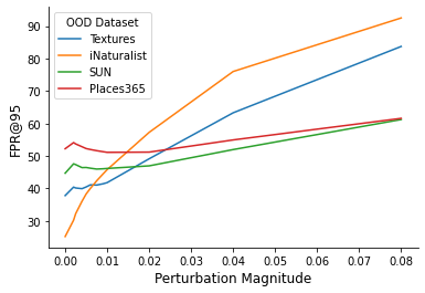
Figure 5: Performance of AbeT with input perturbation. This shows our method using input perturbations from ODIN (Liang et al., 2017). The x-axis is different perturbation magnitudes, and the y-axis is FPR@95 (lower is better). A ResNetv2-101 was trained on ImageNet-1k (Krizhevsky, 2009). For three of the OOD datasets, adding any perturbation hurts performance. For Places365, adding in low levels of perturbation slightly improves performance.

Appendix C Understanding AbeT

C.1 Empirical Evidence

For the following experiments, our embeddings are based on the penultimate representations of a ResNet-20 (He et al., 2016a) trained with learned temperature and a Cosine Logit on CIFAR-10 (Krizhevsky, 2009). Note that these representations are not TSNE-reduced (Van der Maaten & Hinton, 2008), since we do not aim to visualize them:

1. To empirically support that the proportion of points which are near OOD and misclassified is higher than the proportion of points which are misclassified overall, we took the single nearest neighbor in the entire ID test set for each of the OOD Places365 (Zhou et al., 2018) points in embedding space, and found that the ID accuracy on this set of OOD-proximal ID test points was $76.42\%$ compared to $91.89\%$ on all points.

2. To empirically support that misclassified ID test points have OOD scores closer to 0 than correctly classified ID test points, we found that the $99\%$ confidence intervals of the OOD scores on misclassified and correctly classified ID CIFAR-10 (Krizhevsky, 2009) are as follows, respectively: $-20.88\pm 0.57$ and $-33.29\pm.93$.

Appendix D Experimental Details

D.1 Datasets

D.1.1 Classification Datasets

The following information is partially taken directly from Huang et al. (2021), as the details of the datasets used in our experiments are identical to the details of the datasets used in their experiments:

Large-scale evaluation     We use ImageNet-1k (Huang & Li, 2021) as the ID dataset, and evaluate on four OOD test datasets following the setup in (Huang et al., 2021):

• iNaturalist (Van Horn et al., 2018) contains 859,000 plant and animal images across over 5,000 different species. Each image is resized to have a max dimension of 800 pixels. We evaluate on 10,000 images randomly sampled from 110 classes that are disjoint from ImageNet-1k: Coprosma lucida, Cucurbita foetidissima, Mitella diphylla, Selaginella bigelovii, Toxicodendron vernix, Rumex obtusifolius, Ceratophyllum demersum, Streptopus amplexifolius, Portulaca oleracea, Cynodon dactylon, Agave lechuguilla, Pennantia corymbosa, Sapindus saponaria, Prunus serotina, Chondracanthus exasperatus, Sambucus racemosa, Polypodium vulgare, Rhus integrifolia, Woodwardia areolata, Epifagus virginiana, Rubus idaeus, Croton setiger, Mammillaria dioica, Opuntia littoralis, Cercis canadensis, Psidium guajava, Asclepias exaltata, Linaria purpurea, Ferocactus wislizeni, Briza minor, Arbutus menziesii, Corylus americana, Pleopeltis polypodioides, Myoporum laetum, Persea americana, Avena fatua, Blechnum discolor, Physocarpus capitatus, Ungnadia speciosa, Cercocarpus betuloides, Arisaema dracontium, Juniperus californica, Euphorbia prostrata, Leptopteris hymenophylloides, Arum italicum, Raphanus sativus, Myrsine australis, Lupinus stiversii, Pinus echinata, Geum macrophyllum, Ripogonum scandens, Echinocereus triglochidiatus, Cupressus macrocarpa, Ulmus crassifolia, Phormium tenax, Aptenia cordifolia, Osmunda claytoniana, Datura wrightii, Solanum rostratum, Viola adunca, Toxicodendron diversilobum, Viola sororia, Uropappus lindleyi, Veronica chamaedrys, Adenocaulon bicolor, Clintonia uniflora, Cirsium scariosum, Arum maculatum, Taraxacum officinale officinale, Orthilia secunda, Eryngium yuccifolium, Diodia virginiana, Cuscuta gronovii, Sisyrinchium montanum, Lotus corniculatus, Lamium purpureum, Ranunculus repens, Hirschfeldia incana, Phlox divaricata laphamii, Lilium martagon, Clarkia purpurea, Hibiscus moscheutos, Polanisia dodecandra, Fallugia paradoxa, Oenothera rosea, Proboscidea louisianica, Packera glabella, Impatiens parviflora, Glaucium flavum, Cirsium andersonii, Heliopsis helianthoides, Hesperis matronalis, Callirhoe pedata, Crocosmia × crocosmiiflora, Calochortus albus, Nuttallanthus canadensis, Argemone albiflora, Eriogonum fasciculatum, Pyrrhopappus pauciflorus, Zantedeschia aethiopica, Melilotus officinalis, Peritoma arborea, Sisyrinchium bellum, Lobelia siphilitica, Sorghastrum nutans, Typha domingensis, Rubus laciniatus, Dichelostemma congestum, Chimaphila maculata, Echinocactus texensis

• SUN (Xiao et al., 2010) contains over 130,000 images of scenes spanning 397 categories. SUN and ImageNet-1k have overlapping categories. We evaluate on 10,000 images randomly sampled from 50 classes that are disjoint from ImageNet labels: badlands, bamboo forest, bayou, botanical garden, canal (natural), canal (urban), catacomb, cavern (indoor), cornfield, creek, crevasse, desert (sand), desert (vegetation), field (cultivated), field (wild), fishpond, forest (broadleaf), forest (needle leaf), forest path, forest road, hayfield, ice floe, ice shelf, iceberg, islet, marsh, ocean, orchard, pond, rainforest, rice paddy, river, rock arch, sky, snowfield, swamp, tree farm, trench, vineyard, waterfall (block), waterfall (fan), waterfall (plunge), wave, wheat field, herb garden, putting green, ski slope, topiary garden, vegetable garden, formal garden

• Places365 (Zhou et al., 2018) is another scene dataset with similar concept coverage as SUN. A chosen subset of 10,000 images across 50 classes (not contained in ImageNet-1k) are used: badlands, bamboo forest, canal (natural), canal (urban), cornfield, creek, crevasse, desert (sand), desert (vegetation), desert road, field (cultivated), field (wild), field road, forest (broadleaf), forest path, forest road, formal garden, glacier, grotto, hayfield, ice floe, ice shelf, iceberg, igloo, islet, japanese garden, lagoon, lawn, marsh, ocean, orchard, pond, rainforest, rice paddy, river, rock arch, ski slope, sky, snowfield, swamp, swimming hole, topiary garden, tree farm, trench, tundra, underwater (ocean deep), vegetable garden, waterfall, wave, wheat field

• Textures (Cimpoi et al., 2014) contains 5,640 real-world texture images under 47 categories. We use the entire dataset for evaluation.

CIFAR benchmark     CIFAR-10 and CIFAR-100 (Krizhevsky, 2009) are widely used as ID datasets in the literature, which contain 10 and 100 classes, respectively. We use the standard split with 50,000 training images and 10,000 test images. We evaluate our approach on four common OOD datasets, which are listed below:

• SVHN (Netzer et al., 2011) contains color images of house numbers. There are ten classes of digits 0-9. We use the entire test set containing 26,032 images.

• LSUN C (Yu et al., 2015) contains 10,000 testing images across 10 different scenes. Image patches of size 32×32 are randomly cropped from this dataset.

• Places365 (Zhou et al., 2018) contains large-scale photographs of scenes with 365 scene categories. There are 900 images per category in the test set. We randomly sample 10,000 images from the test set for evaluation.

• Textures (Cimpoi et al., 2014) contains 5,640 real-world texture images under 47 categories. We use the entire dataset for evaluation. test set for evaluation.

D.1.2 Semantic Segmentation Datasets

For semantic segmentation experiments, we treat Mapillary (Neuhold et al., 2017) and Cityscapes (Cordts et al., 2016) as the ID datasets and LostAndFound (Pinggera et al., 2016) and RoadAnomaly (Lis et al., 2019) as the OOD datasets.

• Mapillary Vistas (Neuhold et al., 2017) is an urban street scenes dataset consisting of 25,000 images with labels spanning 124 categories intended for autonomous driving. The dataset provides examples covering 6 continents and a variety of weathers and seasons.

• Cityscapes (Cordts et al., 2016) is an urban street scenes dataset consisting of 5,000 images with fine annotations and an additional 20,000 images with coarse annotations. The dataset covers 30 semantic classes and covers 50 cities over several seasons.

• LostAndFound (Pinggera et al., 2016) is an urban street scene dataset comprising of 1203 real images which contain roads with anomalous objects like cones, boxes, tires, or toys. The dataset spans 13 different scenes and features 37 different types of anomalous objects and provides labels for the road, anomalous objects, and background.

• RoadAnomaly (Lis et al., 2019) is a rural street scene dataset comprised of 60 web-scraped images of rural roads with obstacles like zebras, cows, or sheep. The varied scale and size of the anomalous objects, in addition to the rural background, make this dataset very difficult for OOD detection methods.

D.1.3 Object Detection Datasets

• PASCAL VOC (Everingham et al., 2010) is a natural image object detection dataset that contains 20 different object classes. The dataset contains 2,913 distinct images.

• COCO (Lin et al., 2014a) is a large scale object detection dataset. It contains 91 different object categories with over 200,000 labelled images. Image resolution of this dataset is 640 x 480.

D.2 Models and Hyperparameters

D.2.1 Classification Models and Hyperparameters

For all CIFAR experiments, we trained with a batch size of 64 and - identical to Huang et al. (2021) - with an initial learning rate of $0.1$ which decays by a factor of $10$ at epochs $50\%,75\%,$ and $90\%$ of total epochs. For all Imagenet experiments, we trained with a batch size of 512 with an initial learning rate of $0.1$ which decays by a factor of $10$ at epochs $20$ and $30$. For our CIFAR and ImageNet experiments we train for 200 and 40 total epochs respectively without early stopping or validation saving. For CIFAR experiments, we use Horizontal Flipping and Trivial Augment Wide (Müller & Hutter, 2021). For Imagenet experiments, we use the augmentations from Torchvision’s recipe (TODO: cite blog https://pytorch.org/blog/how-to-train-state-of-the-art-models-using-torchvision-latest-primitives/).

D.2.2 Semantic Segmentation Models and Hyperparameters

For all semantic segmentation experiements, we utilize the DeepLabv3+ segmentation model with a WideResnet38 backbone (Zhu et al., 2019; Reda et al., 2018). All models are pretrained on Mapillary (Neuhold et al., 2017) and finetuned on Cityscapes (Cordts et al., 2016). For comparison methods, we use the we use the publicly available weights (Reda et al., 2018) as the pretrained model. For our method, in order to incorporate our Cosine Logit head and learned temperature layer, we trained a new model from scratch following the exact training in (Zhu et al., 2019; Reda et al., 2018). This consists of a pretraining stage on Mapillary, which trains for a maximum of 175 epochs with an initial learning rate of 0.02, decaying each epoch by a factor of $(1-\frac{epoch}{max\_epoch})$. Additionally, several advanced training techniques are used, such as class uniform sampling, augmentations like random cropping and Gaussian blur, Synchronized Batch Normalization, and a special inverse-target-frequency weighted cross-entropy loss. Once the Mapillary pretrained model reaches a mIOU of $\geq 0.5$, the Cityscapes finetuning training begins. The Cityscapes finetuning consists of training for a maximum of 175 epochs with an initial learning rate of 0.001, which begins to decay by a factor of $1-\frac{epoch}{max\_epoch}$ each epoch until epoch 100, at which point the learning rate decays by $(1-\frac{epoch-100}{max\_epoch-100})^{1.5}$ per epoch. The same advanced training techniques as above are utilized, except with a custom loss function designed to reach greater accuracy on borders between classes. The finetuning is considered finished when the model reached a Cityscapes Validation mIOU $\geq 0.8$. We do not utilize their optional additional training step using label propogation via video prediction and the Cityscape sequences dataset due to compute constraints. For more specifics about training, visit https://github.com/NVIDIA/semantic-segmentation/tree/sdcnet (TODO: hyperlink). For both the Mapillary pretraining and the Cityscapes finetuning, we utilize a batch size of 8 on 8 NVIDIA T4 GPUs and conduct all training in half-precision for speed.

For evaluation, we utilize the code and framework from Chan et al. (2021), which uses a histogram approach to avoid memory errors while calculating statistics over thousands of images. OOD scores are normalized to a range of $[0,1]$, then bucketed into either the ID histogram or OOD histogram of 100 even spaced bins spanning $[0,1]$ depending on their label. For example, entropy scores are normalized to $[0,1]$ by dividing the entropy scores by the logarithm of the number of classes. At this point, we invert some scoring methods like MSP (using an inversion that exactly reverses the ordering of points according to OOD score) so that all methods align with the framework of ID scores near 0 and OOD scores near 1. Once all the scores have been added to their respective histograms, the counts are normalized by a maximum value, chosen as $10^{7}$, then transformed back into lists of predictions according to their bin value. Statistics like FPR@95, AUROC, and AUPRC are calculated on this list of scores, which drastically drops the runtime while maintaining the correct distribution. For further details on evaluation techniques, see Chan et al. (2021).

D.2.3 Object Detection Models and Hyperparameters

For all object detection experiments, we utilize the detectron2 package in order to train a FasterRCNN with a ResNet50 backbone pretrained on ImageNet. All models were trained with a batch size of 4. During training, images were augmented with random croppinxg and flipping. A base learning rate of 0.02 was used and decays at steps 12,000 and 16,000 per the setup in (Du et al., 2022). All models were trained on an Nvidia V100 GPU for a maximum of 18,000 iterations, where only the model with the best validation loss was saved.

Appendix E Classification Baseline Methods

E.1 Hyperparameters

For all previous approaches, we use the default hyperparameters described in their respective papers, other than for our CIFAR-10 experiment we use $K=200$ for Deep Nearest Neighbors (Sun et al., 2022), as we found it to reduce FPR@95 by $12.40\%$ as compared to the default $K=50$ in the paper. For our ImageNet experiments for Deep Nearest Neighbors (Sun et al., 2022), we use a sampling ratio of $1\%$ for runtime memory reasons.

E.2 Descriptions

For the reader’s convenience, we summarize in detail a few common techniques for defining OOD scores in classification that measure the degree of ID-ness on the given sample. Some of these descriptions are taken directly from Huang et al. (2021).

The following scores follow a convention that a higher (resp. lower) score is indicative of being ID (resp. OOD):

MSP Hendrycks & Gimpel (2016) propose to use the maximum softmax score to detect OOD samples.

ODIN Liang et al. (2017) improved OOD detection with temperature scaling and input perturbation. Note that this is different from calibration, where a much milder T will be employed. While calibration focuses on representing the true correctness likelihood of ID data, the OOD scores proposed by ODIN are designed to maximize the gap between ID and OOD data and may no longer be meaningful from a predictive confidence standpoint.

GODIN Hsu et al. (2020) substitutes the temperature scaling with the use of a explicit variable $d_{in}$ in the classifier, rewriting the class posterior probability as the quotient of the joint class-domain probability and the domain probability using the rule of conditional probability $p(y|d_{in},x_{i})=\frac{p(y,d_{in}|x_{i})}{p(d_{in}|x_{i})}$. GODIN uses this dividend/divisor structure to define a logit per class as the division of two functions $f_{j}(x)=\frac{h_{j}(x)}{g_{j}(x)}$. The learned $h$ and $g$ from ID map well to the quotient decomposition above, and are used as the OOD score. We found using $g_{j}(x)$ as the OOD score to be the most performant on average, and thus we use this divisor as the GODIN OOD score for all experiments. We additionally do not perform backward-pass-based input perturbations with GODIN, as we found them to harm OOD performance - similar to the findings of Huang et al. (2021) on ODIN. This is equivalent to setting $\epsilon=0$.

DICE Sun & Li (2021) proposes a sparsification-based OOD detection framework. The key idea is to rank weights in the penultimate layer based on a measure of contribution, and selectively use the most salient weights to derive the output for OOD detection. For ID data, only a subset of units contributes to the model output. In contrast, OOD data can trigger a non-negligible fraction of units with noisy signals. To exploit this, DICE ranks weights based on the measure of contribution (weight x activation), and selectively uses the most contributing weights to derive the output for OOD detection. As a result of the weight sparsification, the model’s output becomes more separable between ID and OOD data. Importantly, DICE can be conveniently used by post hoc weight masking on a pre-trained network and therefore can preserve the ID classification accuracy.

ReAct In the penultimate layer, the mean activation for ID data is well-behaved with a near-constant mean and standard deviation. In contrast, for OOD data, the mean activation has significantly larger variations across units and is biased towards having sharp positive values (i.e., positively skewed). As a result, such high unit activation can undesirably manifest in model output, producing overconfident predictions on OOD data. The method Rectified Activations (dubbed ReAct, proposed by Sun et al. (2021)) uses the above observation for OOD detection. In particular, the outsized activation of a few selected hidden units can be attenuated by rectifying the activations at an upper limit $c>0$. Conveniently, this can be done on a pre-trained model without any modification to training. After rectification, the output distributions for ID and OOD data become much more well-separated. Importantly, this truncation largely preserves the activation for ID data, and therefore ensures the classification accuracy on the original task is largely comparable.

Max Logit (Hendrycks et al., 2022) attempts to address a shortcoming of MSP where the softmax operator may redistribute probability mass among several large logits. In the case of two large logits, their relative maximum is lowered by the softmax operator as they must split the probability mass. The Max Logit approach is to simply observe the maximum logit as the OOD score instead of the maximum softmax probability.

Standardized Max Logit (Jung et al., 2021) improves upon the Max Logit approach by observing that the distribution of max logits for each class is significantly different from one another. The SML approach is to standardize the max logit scores on a per-class basis using the ID dataset to collect expected means and variances. These per-class means and variances are then used during OOD evaluation, with the Z-score of the respective max logit for each prediction used as the OOD score.

The following scores follow a convention that a higher (resp. lower) score is indicative of being OOD (resp. ID):

Energy Liu et al. (2020) first proposed using energy score for OOD uncertainty estimation. The energy function maps the logit outputs to a scalar $S_{Energy}(x_{i};f)\in R$, which is relatively more negative for ID data $S_{Energy}(x_{i};f)=-T\log\sum\limits_{j=1}^{C}e^{f_{j}(x_{i})/T}$. We compare against the version of Energy Score which is not fine-tuned on OOD data at training time, as training on OOD data would violate our assumption that we do not have access to OOD data at training time.

Mahalanobis Lee et al. (2018) use multivariate Gaussian distributions to model class-conditional distributions in the penultimate layer and use Mahalanobis distance-based scores to these distributions for OOD detection.

Entropy (Chan et al., 2021) propose using the entropy of the softmax probabilities as the scoring method for OOD detection. They propose the discrete entropy formula $E(f(x))=-\sum_{j\in C}f_{j}(x)log(f_{j}(x))$, where $f_{j}$ represents the softmax probability over each class $j\in C$. This method sees strong performance when paired with OOD finetuning where the model is forced to learn to output uniform probabilities on OOD examples in order to maximize the entropy of those predictions.

Deep Nearest Neighbors Methods like (Lee et al., 2018) make a strong distributional assumption of the underlying feature space being class-conditional Gaussian. Sun et al. (2022) explore the efficacy of non-parametric nearest-neighbor distance for OOD detection. In particular, they use the distance to the k-th nearest neighbor in the penultimate space of the training set as their OOD score. We compare against the version of Deep Nearest Neighbors which does train a representation network via Supervised Contrastive Loss (Khosla et al., 2020). Training a representation network with Supervised Contrastive Loss would modify training to violate our assumption that we only train in a single stage, as there would be a required second training stage which fits a model that maps these representations to logit space $\mathbb{R}^{C}$.

References

- Chan et al. (2021) Robin Chan, Matthias Rottmann, and Hanno Gottschalk. Entropy maximization and meta classification for out-of-distribution detection in semantic segmentation. In Proceedings of the ieee/cvf international conference on computer vision, pp. 5128–5137, 2021.
- Cimpoi et al. (2014) Mircea Cimpoi, Subhransu Maji, Iasonas Kokkinos, Sammy Mohamed, and Andrea Vedaldi. Describing textures in the wild. In Proceedings of the IEEE conference on computer vision and pattern recognition, pp. 3606–3613, 2014.
- Cordts et al. (2016) Marius Cordts, Mohamed Omran, Sebastian Ramos, Timo Rehfeld, Markus Enzweiler, Rodrigo Benenson, Uwe Franke, Stefan Roth, and Bernt Schiele. The cityscapes dataset for semantic urban scene understanding. In Proc. of the IEEE Conference on Computer Vision and Pattern Recognition (CVPR), 2016.
- Dai et al. (2016) Jifeng Dai, Yi Li, Kaiming He, and Jian Sun. R-fcn: Object detection via region-based fully convolutional networks. In Advances in neural information processing systems, pp. 379–387, 2016.
- Devlin et al. (2018) Jacob Devlin, Ming-Wei Chang, Kenton Lee, and Kristina Toutanova. Bert: Pre-training of deep bidirectional transformers for language understanding. arXiv preprint arXiv:1810.04805, 2018.
- Djurisic et al. (2022) Andrija Djurisic, Nebojsa Bozanic, Arjun Ashok, and Rosanne Liu. Extremely simple activation shaping for out-of-distribution detection. arXiv preprint arXiv:2209.09858, 2022.
- Dosovitskiy et al. (2020) Alexey Dosovitskiy, Lucas Beyer, Alexander Kolesnikov, Dirk Weissenborn, Xiaohua Zhai, Thomas Unterthiner, Mostafa Dehghani, Matthias Minderer, Georg Heigold, Sylvain Gelly, et al. An image is worth 16x16 words: Transformers for image recognition at scale. arXiv preprint arXiv:2010.11929, 2020.
- Du et al. (2022) Xuefeng Du, Zhaoning Wang, Mu Cai, and Yixuan Li. Vos: Learning what you don’t know by virtual outlier synthesis. arXiv preprint arXiv:2202.01197, 2022.
- Everingham et al. (2010) Mark Everingham, Luc Van Gool, Christopher K. I. Williams, John M. Winn, and Andrew. Zisserman. The pascal visual object classes (voc) challenge. In International Journal of Computer Vision, pp. 303–338, 2010.
- Feichtenhofer (2020) Christoph Feichtenhofer. X3d: Expanding architectures for efficient video recognition. In Proceedings of the IEEE/CVF Conference on Computer Vision and Pattern Recognition, pp. 203–213, 2020.
- Girshick (2015) Ross Girshick. Fast r-cnn. In Proceedings of the IEEE international conference on computer vision, pp. 1440–1448, 2015.
- Guo et al. (2017) Chuan Guo, Geoff Pleiss, Yu Sun, and Kilian Q Weinberger. On calibration of modern neural networks. In Proceedings of the 34th International Conference on Machine Learning-Volume 70, pp. 1321–1330. JMLR. org, 2017.
- He et al. (2016a) Kaiming He, Xiangyu Zhang, Shaoqing Ren, and Jian Sun. Deep residual learning for image recognition. In 2016 IEEE Conference on Computer Vision and Pattern Recognition (CVPR), pp. 770–778, 2016a. doi: 10.1109/CVPR.2016.90.
- He et al. (2016b) Kaiming He, Xiangyu Zhang, Shaoqing Ren, and Jian Sun. Identity mappings in deep residual networks. In European conference on computer vision, pp. 630–645. Springer, 2016b.
- Hendrycks & Gimpel (2016) Dan Hendrycks and Kevin Gimpel. A baseline for detecting misclassified and out-of-distribution examples in neural networks. arXiv preprint arXiv:1610.02136, 2016.
- Hendrycks et al. (2018) Dan Hendrycks, Mantas Mazeika, and Thomas Dietterich. Deep anomaly detection with outlier exposure. arXiv preprint arXiv:1812.04606, 2018.
- Hendrycks et al. (2022) Dan Hendrycks, Steven Basart, Mantas Mazeika, Andy Zou, Joseph Kwon, Mohammadreza Mostajabi, Jacob Steinhardt, and Dawn Song. Scaling out-of-distribution detection for real-world settings. In ICML, pp. 8759–8773, 2022. URL https://proceedings.mlr.press/v162/hendrycks22a.html.
- Hsu et al. (2020) Yen-Chang Hsu, Yilin Shen, Hongxia Jin, and Zsolt Kira. Generalized odin: Detecting out-of-distribution image without learning from out-of-distribution data. In Proceedings of the IEEE/CVF Conference on Computer Vision and Pattern Recognition, pp. 10951–10960, 2020.
- Huang et al. (2017) Gao Huang, Zhuang Liu, Laurens Van Der Maaten, and Kilian Q Weinberger. Densely connected convolutional networks. In Proceedings of the IEEE conference on computer vision and pattern recognition, pp. 4700–4708, 2017.
- Huang & Li (2021) Rui Huang and Yixuan Li. Mos: Towards scaling out-of-distribution detection for large semantic space. In Proceedings of the IEEE/CVF Conference on Computer Vision and Pattern Recognition, pp. 8710–8719, 2021.
- Huang et al. (2021) Rui Huang, Andrew Geng, and Yixuan Li. On the importance of gradients for detecting distributional shifts in the wild. Advances in Neural Information Processing Systems, 34:677–689, 2021.
- Jung et al. (2021) Sanghun Jung, Jungsoo Lee, Daehoon Gwak, Sungha Choi, and Jaegul Choo. Standardized max logits: A simple yet effective approach for identifying unexpected road obstacles in urban-scene segmentation. In Proceedings of the IEEE/CVF International Conference on Computer Vision (ICCV), pp. 15425–15434, October 2021.
- Katz-Samuels et al. (2022) Julian Katz-Samuels, Julia B Nakhleh, Robert Nowak, and Yixuan Li. Training ood detectors in their natural habitats. In International Conference on Machine Learning, pp. 10848–10865. PMLR, 2022.
- Khalid et al. (2022) Umar Khalid, Ashkan Esmaeili, Nazmul Karim, and Nazanin Rahnavard. Rodd: A self-supervised approach for robust out-of-distribution detection. arXiv preprint arXiv:2204.02553, 2022.
- Khosla et al. (2020) Prannay Khosla, Piotr Teterwak, Chen Wang, Aaron Sarna, Yonglong Tian, Phillip Isola, Aaron Maschinot, Ce Liu, and Dilip Krishnan. Supervised contrastive learning. Advances in Neural Information Processing Systems, 33:18661–18673, 2020.
- Krizhevsky (2009) Alex Krizhevsky. Learning multiple layers of features from tiny images. Technical report, none, 2009.
- Lee et al. (2018) Kimin Lee, Kibok Lee, Honglak Lee, and Jinwoo Shin. A simple unified framework for detecting out-of-distribution samples and adversarial attacks. In Advances in Neural Information Processing Systems, pp. 7167–7177, 2018.
- Liang et al. (2017) Shiyu Liang, Yixuan Li, and Rayadurgam Srikant. Enhancing the reliability of out-of-distribution image detection in neural networks. arXiv preprint arXiv:1706.02690, 2017.
- Lin et al. (2014a) Tsung-Yi Lin, Michael Maire, Serge Belongie, James Hays, Belongie Perona, Deva Ramanan, Piotr Dollar, , and C Lawrence. Zitnick. Microsoft coco: Common objects in context. In European conference on computer vision, pp. 740–755, 2014a.
- Lin et al. (2014b) Tsung-Yi Lin, Michael Maire, Serge J. Belongie, James Hays, Pietro Perona, Deva Ramanan, Piotr Dollár, and C. Lawrence Zitnick. Microsoft coco: Common objects in context. In European Conference on Computer Vision, 2014b.
- Lin et al. (2017) Tsung-Yi Lin, Priya Goyal, Ross Girshick, Kaiming He, and Piotr Dollár. Focal loss for dense object detection. In Proceedings of the IEEE international conference on computer vision, pp. 2980–2988, 2017.
- Lis et al. (2019) Krzysztof Lis, Krishna Nakka, Pascal Fua, and Mathieu Salzmann. Detecting the unexpected via image resynthesis. In In Proceedings of the IEEE International Conference on Computer Vision, pp. 2152–2161, 2019.
- Liu et al. (2016) Wei Liu, Dragomir Anguelov, Dumitru Erhan, Christian Szegedy, Scott Reed, Cheng-Yang Fu, and Alexander C Berg. Ssd: Single shot multibox detector. In European conference on computer vision, pp. 21–37. Springer, 2016.
- Liu et al. (2020) Weitang Liu, Xiaoyun Wang, John Owens, and Yixuan Li. Energy-based out-of-distribution detection. Advances in Neural Information Processing Systems, 33:21464–21475, 2020.
- Ming et al. (2022) Yifei Ming, Ying Fan, and Yixuan Li. POEM: Out-of-distribution detection with posterior sampling. In Kamalika Chaudhuri, Stefanie Jegelka, Le Song, Csaba Szepesvari, Gang Niu, and Sivan Sabato (eds.), Proceedings of the 39th International Conference on Machine Learning, volume 162 of Proceedings of Machine Learning Research, pp. 15650–15665. PMLR, 17–23 Jul 2022. URL https://proceedings.mlr.press/v162/ming22a.html.
- Mukhoti & Gal (2018) Jishnu Mukhoti and Yarin Gal. Evaluating bayesian deep learning methods for semantic segmentation. arXiv preprint arXiv:1811.12709, 2018.
- Müller & Hutter (2021) Samuel G Müller and Frank Hutter. Trivialaugment: Tuning-free yet state-of-the-art data augmentation. In Proceedings of the IEEE/CVF International Conference on Computer Vision, pp. 774–782, 2021.
- Netzer et al. (2011) Yuval Netzer, Tao Wang, Adam Coates, Alessandro Bissacco, Bo Wu, and Andrew Y. Ng. Reading digits in natural images with unsupervised feature learning. In NIPS Workshop on Deep Learning and Unsupervised Feature Learning 2011, 2011. URL http://ufldl.stanford.edu/housenumbers/nips2011_housenumbers.pdf.
- Neuhold et al. (2017) Gerhard Neuhold, Tobias Ollmann, Samuel Rota Bulo, and Peter Kontschieder. The mapillary vistas dataset for semantic understanding of street scenes. In Proceedings of the IEEE International Conference on Computer Vision (ICCV), Oct 2017.
- Nguyen et al. (2015) Anh Nguyen, Jason Yosinski, and Jeff Clune. Deep neural networks are easily fooled: High confidence predictions for unrecognizable images. In Proceedings of the IEEE conference on computer vision and pattern recognition, pp. 427–436, 2015.
- Ovadia et al. (2019) Yaniv Ovadia, Emily Fertig, Jie Ren, Zachary Nado, David Sculley, Sebastian Nowozin, Joshua Dillon, Balaji Lakshminarayanan, and Jasper Snoek. Can you trust your model’s uncertainty? evaluating predictive uncertainty under dataset shift. Advances in neural information processing systems, 32, 2019.
- Pinggera et al. (2016) Peter Pinggera, Sebastian Ramos, Stefan Gehrig, Uwe Franke, Carsten Rother, and Rudolf Mester. Lost and found: detecting small road hazards for self-driving vehicles. In In Proceedings of IEEE/RSJ International Conference on Intelligent Robots and Systems, pp. 1099–1106, 2016.
- Radford et al. (2021) Alec Radford, Jong Wook Kim, Chris Hallacy, Aditya Ramesh, Gabriel Goh, Sandhini Agarwal, Girish Sastry, Amanda Askell, Pamela Mishkin, Jack Clark, et al. Learning transferable visual models from natural language supervision. In International Conference on Machine Learning, pp. 8748–8763. PMLR, 2021.
- Reda et al. (2018) Fitsum A Reda, Guilin Liu, Kevin J Shih, Robert Kirby, Jon Barker, David Tarjan, Andrew Tao, and Bryan Catanzaro. Sdc-net: Video prediction using spatially-displaced convolution. In Proceedings of the European Conference on Computer Vision (ECCV), pp. 718–733, 2018.
- Redmon et al. (2016) Joseph Redmon, Santosh Divvala, Ross Girshick, and Ali Farhadi. You only look once: Unified, real-time object detection. In Proceedings of the IEEE conference on computer vision and pattern recognition, pp. 779–788, 2016.
- Ren et al. (2015) Shaoqing Ren, Kaiming He, Ross Girshick, and Jian Sun. Faster r-cnn: Towards real-time object detection with region proposal networks. In Advances in neural information processing systems, pp. 91–99, 2015.
- Sun & Li (2021) Yiyou Sun and Yixuan Li. On the effectiveness of sparsification for detecting the deep unknowns. arXiv preprint arXiv:2111.09805, 2021.
- Sun et al. (2021) Yiyou Sun, Chuan Guo, and Yixuan Li. React: Out-of-distribution detection with rectified activations. Advances in Neural Information Processing Systems, 34:144–157, 2021.
- Sun et al. (2022) Yiyou Sun, Yifei Ming, Xiaojin Zhu, and Yixuan Li. Out-of-distribution detection with deep nearest neighbors. arXiv preprint arXiv:2204.06507, 2022.
- Tian et al. (2022) Yu Tian, Yuyuan Liu, Guansong Pang, Fengbei Liu, Yuanhong Chen, and Gustavo Carneiro. Pixel-wise energy-biased abstention learning for anomaly segmentation on complex urban driving scenes. In none, pp. 246–263, 10 2022.
- Van der Maaten & Hinton (2008) Laurens Van der Maaten and Geoffrey Hinton. Visualizing data using t-sne. Journal of machine learning research, 9(11), 2008.
- Van Horn et al. (2018) Grant Van Horn, Oisin Mac Aodha, Yang Song, Yin Cui, Chen Sun, Alex Shepard, Hartwig Adam, Pietro Perona, and Serge Belongie. The inaturalist species classification and detection dataset. In Proceedings of the IEEE conference on computer vision and pattern recognition, pp. 8769–8778, 2018.
- Xiao et al. (2010) Jianxiong Xiao, James Hays, Krista A. Ehinger, Aude Oliva, and Antonio Torralba. Sun database: Large-scale scene recognition from abbey to zoo. In 2010 IEEE Computer Society Conference on Computer Vision and Pattern Recognition, pp. 3485–3492, 2010. doi: 10.1109/CVPR.2010.5539970.
- Yu et al. (2015) Fisher Yu, Ari Seff, Yinda Zhang, Shuran Song, Thomas Funkhouser, and Jianxiong Xiao. Lsun: Construction of a large-scale image dataset using deep learning with humans in the loop. arXiv preprint arXiv:1506.03365, 2015.
- Zhou et al. (2018) Bolei Zhou, Agata Lapedriza, Aditya Khosla, Aude Oliva, and Antonio Torralba. Places: A 10 million image database for scene recognition. IEEE Transactions on Pattern Analysis and Machine Intelligence, 40(6):1452–1464, 2018. doi: 10.1109/TPAMI.2017.2723009.
- Zhu et al. (2019) Yi Zhu, Karan Sapra, Fitsum A. Reda, Kevin J. Shih, Shawn Newsam, Andrew Tao, and Bryan Catanzaro. Improving semantic segmentation via video propagation and label relaxation. In IEEE Conference on Computer Vision and Pattern Recognition (CVPR), June 2019. URL https://nv-adlr.github.io/publication/2018-Segmentation.