Centralization in Block Building and Proposer-Builder Separation

Abstract

The goal of this paper is to rigorously interrogate conventional wisdom about centralization in block-building (due to, e.g., MEV and private order flow) and the outsourcing of block-building by validators to specialists (i.e., proposer-builder separation):

1. Does heterogeneity in skills and knowledge across block producers inevitably lead to centralization?

2. Does proposer-builder separation eliminate heterogeneity and preserve decentralization among proposers?

This paper develops mathematical models and results that offer answers to these questions:

1. In a game-theoretic model with endogenous staking, heterogeneous block producer rewards, and staking costs, we quantify the extent to which heterogeneous rewards lead to concentration in the equilibrium staking distribution.

2. In a stochastic model in which heterogeneous block producers repeatedly reinvest rewards into staking, we quantify, as a function of the block producer heterogeneity, the rate at which stake concentrates on the most sophisticated block producers.

3. In a model with heterogeneous proposers and specialized builders, we quantify, as a function of the competitiveness of the builder ecosystem, the extent to which proposer-builder separation reduces the heterogeneity in rewards across different proposers.

Our models and results take advantage of connections to contest design, Pólya urn processes, and auction theory.

1 Introduction

Heterogeneity in rewards for block production.

The economics of block production for blockchain protocols has been growing increasingly complex over time, with block producers earning revenue from an increasing number of different sources. For example, when the Bitcoin and Ethereum protocols first launched, there was minimal demand for blockspace and minimal activity at the application layer. Publishing a block netted a fixed block reward for the miner or validator that produced it but little other revenue. In this regime, the frequency of block production varies across block producers (according to the hashrate or stake invested in the protocol), but the per-block reward does not.

In time, demand for blockspace exceeded supply, forcing users to pay non-negligible transaction fees in exchange for transaction inclusion. Block producers were then incentivized to publish a block with the maximum-possible sum of transaction fees. In this case, if all transactions are visible to all block producers (e.g., in a public mempool), the value of a block production opportunity would remain the same across potential block producers (namely, the block reward plus the revenue-maximizing packing of pending transactions). If not all block producers are aware of the same transactions, however—perhaps because some transactions were submitted privately to one or a subset of potential block producers—different block producers might be able to extract differing amounts of revenue from the same block production opportunity.

The rise of decentralized finance (“DeFi”) and the consequent opportunities for value extraction from the application layer (“miner/maximal extractible value,” or “MEV”) appears to have exacerbated the gap in revenue that can be earned by the most and least capable block producers [26, 14]. A block producer with exclusive access to high-value DeFi transactions and a proprietary and computationally intensive algorithm to assemble them into blocks will generally earn much more from a block production opportunity than, for example, a hobbyist running the protocol’s reference client on their home computer .

The centralizing forces of heterogeneity.

Why does it matter? One concern is that heterogeneity in information and skill across potential block producers could lead to “centralization,” with the blockchain protocol ultimately run by only a very small number of the most skilled block producers (perhaps operated by some of the world’s largest financial institutions). For example, Buterin [7] writes: “Block production is likely to become a specialized market.” One possible intuition for this prediction is economic: participating in a protocol carries a cost (e.g., in a proof-of-stake protocol, the opportunity cost of staked capital and/or the cost of operating one or more validators) and perhaps only those with the highest return-on-investment will find it profitable. A different intuition stems from long-run dynamics: the block producers that earn the highest rewards will be in a position to increase their control over the protocol (e.g., by reinvesting rewards as additional stake) until none of the other block producers matter. In any case, much of the motivation behind the design of permissionless blockchain protocols like Bitcoin and Ethereum is exactly to avoid this type of centralization.

Confining heterogeneity to block-building.

How could one encourage a large set of diverse participants to contribute to the operation of a blockchain protocol, despite what would seem to be strong forces pushing toward centralization? One widely-discussed idea in the Ethereum ecosystem is “proposer-builder separation (PBS)” [8], in which the role of assembling a (presumably high-revenue) block of transactions is split out from the role of actually participating in the blockchain protocol (validating and proposing blocks, voting on other proposed blocks, etc.). The intuition is that block-building is the part of the block production pipeline that benefits from specialization (private knowledge of transactions, proprietary block-building algorithms, etc.), with a relatively level playing field for everything else (publishing blocks already assembled by builders, voting, etc.). Quoting Buterin [7] again, on the subject of PBS: “This ensures that at least any centralization tendencies in block production don’t lead to a completely elite-captured and concentrated staking pool market dominating block validation.”

One possible implementation of this idea, which is roughly the implementation in Flashbots’s MEV-Boost [12], is for block-builders to submit bids along with blocks. If a block from a builder is published by a proposer, the corresponding bid is transferred from the builder to the proposer. (Presumably, the builder extracts enough value from the block, via transaction fees and/or application-layer value, to cover its bid to the proposer, perhaps plus a premium.) The hope, then, is that builders are good enough at their jobs that no proposer would be able to improve over the obvious strategy of publishing the block accompanied by the highest bid. If all of the block proposers followed this strategy and always knew about the full set of builder-submitted blocks, then the reward earned by a block production opportunity would once again be independent of the selected proposer. Ideally, restoring such homogeneity would allow for a large and diverse set of proposers.

Goal of this paper.

The motivation and objectives for proposer-builder separation described above rest on plausible but largely unsubstantiated beliefs, the rigorous interrogation of which is the goal of this paper.

1. Does heterogeneity in skills and knowledge across block producers inevitably lead to centralization?

   1. Is it economic forces that lead to centralization? If so, to what extent?

   2. Do long-run dynamics lead to centralization? If so, how quickly?

2. To what extent does proposer-builder separation reduce heterogeneity and preserve decentralization among proposers? How does the answer depend on the competitiveness of the builder ecosystem?

1.1 Overview of Results

This paper develops mathematical models and results that offer answers to all of the questions above:

1. Section 3 addresses question 1(a) through a game-theoretic model with endogenous staking, heterogeneous block producer rewards, and staking costs. Building on connections to Tullock contests, the main result (Theorem 3.3) quantifies the extent to which heterogeneous rewards lead to concentration in the equilibrium staking distribution.

2. Section 4 investigates question 1(b) using a stochastic process in which heterogeneous block producers repeatedly reinvest rewards into staking. Building on connections to Pólya urns and Yule processes, the main result (Theorem 4.2) quantifies, as a function of the block producer heterogeneity, the rate at which stake concentrates on the most sophisticated block producers.

3. Section 5 studies question 2 in a model with heterogeneous proposers and specialized builders, with proposers optionally constructing their own blocks on the side. Building on connections to auction theory, the main result (Theorem 5.1) quantifies, as a function of the competitiveness of the builder ecosystem, the extent to which PBS reduces the heterogeneity in rewards across different proposers.

Our results clarify the extent to and the assumptions under which the conventional wisdom around centralization in block-building and PBS is correct. For example, our analysis in Section 3 shows that economic forces generally lead to an oligopolistic equilibrium outcome rather than a naive “winner-take-all” scenario. For another example, our analysis in Section 5 shows that conventional intuition around PBS breaks down if the distribution of block values is sufficiently heavy-tailed.

Our results also provide quantitative predictions that would be impossible without concrete mathematical models. For example, our analysis in Section 3 suggests that if, say, there at least 10 block producers that are at least 90% as good at extracting value as the most sophisticated block producer, then at equilibrium no block producer will control more than roughly 17.5% of the stake. For another example, our analysis in Section 4 suggests that even modest constant-factor decreases in the performance gap between the best and second-best block producers can greatly slow down the rate of stake concentration.

1.2 Related Work

Tullock contests.

Outside the world of blockchains, considerable effort has gone into understanding the equilibria of games in which strategic agents must invest resources to compete for a fixed prize. This type of game, termed a Tullock Contest, was first studied by Tullock [5] for the case of homogeneous agents. That model was then extended by Hillman and Riley [15] and Gradstein [13] for the case with heterogeneous agents that faced different costs of investment. In a separate but closely related line of work, Johari and Tskitlis [18] and Rougharden [23] study equilibria in resource allocation games. Here there is a fixed amount of resource to be distributed and agents make bids for different shares. These models have since been ported to blockchains in [2, 9, 1, 6] to understand how much miners invest in hardware and energy at equilibriun in proof of work blockchains. In particular, Arnosti and Weinberg [2] and Alsabah and Capponi [1] demonstrate that, at equilibirum, the market share of block production becomes centralized amongst the miners that can invest at the cheapest cost. One difference between these works and our analysis in Section 3 is that they focus on heterogeneity in cost of investment while keeping the reward fixed for all miners, while our model has block producers that earn different rewards but with identical costs. A second is our emphasis on parameterized definitions of and sufficient conditions for decentralization (Definition 3.2 and Theorem 3.3).

Proof of stake.

Moving to proof of stake protocols, there have been many works investigating possible rich get richer phenomena, the worry being that block producers who start with a large fraction of the stake will grow their advantage and eventually control all of the stake. Work by Rosu and Saleh [22] shows that in a model in which all block producers earn the same rewards, with these rewards relatively small compared to the absolute amount of stake, the ratio of stake controlled by different block producers follows a martingale, typically keeping them at essentially the same ratio over the long run. Additional work by Huang et al. [16] and Tang [25, 24] reach similar conclusions in somewhat different models of proof of stake protocols. Fanti et al. [11] introduce a notion of equitability that quantifies whether or not block producers maintain the same share of stake over time and they study how different reward functions impact this metric. In all of these works, the reward earned by a block production opportunity is independent of the block producer (i.e., there is no block producer heterogeneity, other than their current stake amounts).

Our work here shows that, by contrast, with heterogeneous block producers, a rich get richer effect does indeed occur, with the block producers capable of earning the highest rewards (per block production opportunity) eventually controlling a dominant fraction of the total stake.

Pólya urns.

Pólya urns are important for our analysis in Section 4 of the long run behavior of the staking process. As noted in several earlier works (without BP heterogeneity) [11, 16, 22, 24, 25], there is a strong resemblance between the Pólya urn setup of repeatedly drawing a ball randomly from an urn and replacing that ball with more balls of the same color and a process in which block producers repeatedly reinvest all earned rewards into staking. Pólya urns were first formally introduced by Eggenberger and Pólya in [10] and there is now a large literature on the topic. Of particular interest to us is a technique of Athreya and Karlin [3] for embedding a discrete Pólya scheme into a continuous Pólya process. Janson [17] built on this work by using the continuous-time process to prove results about the limiting distribution for a wide variety of Pólya urn models, including models with color-specific replacement parameters that correspond to the non-uniform reward rates of heterogeneous BPs in our model. Translated to our model, one of Janson’s results implies that a block producer with a consistent advantage in earning rewards over the other block producers will eventually, in the limit, control all of the stake. Our analysis here builds on Janson’s result to quantify exactly how quickly, as a function of the size of the BP’s advantage, we can expect this concentration to occur.

2 The Basic Model

The focus of this work is on the centralizing effects of block producer heterogeneity. To isolate this issue, this section defines what is arguably a minimal model that allows for its study.

We consider a finite set $I=\{1,2,\ldots,n\}$ of block producers (BPs). Each BP $i\in I$ is characterized by a reward multipler $\mu_{i}\geq 1$; BPs with higher $\mu_{i}$’s earn more from producing a block than those with lower $\mu_{i}$’s. Specifically, we consider a block production opportunity (e.g., a slot in the Ethereum protocol) with “base reward” equal to some value $r>0$ and assume that, if the BP $i$ is the one selected to take advantage of this opportunity (e.g., by winning a proof-of-stake lottery for that slot), then it earns $\mu_{i}r$ from it. We do not model any details of the source(s) of these rewards, which could include a block reward, transaction fees (as computed by some transaction fee mechanism), and/or value derived from the application layer (i.e., “MEV”). We assume that a BP is chosen for a block production opportunity with probability proportional to the amount of the blockchain’s native currency that it has staked at that time. Thus, the expected reward earned by BP $i$ for a given block production opportunity is

$$\frac{\pi_{i}}{\sum_{j\in I}\pi_{j}}\cdot\mu_{i}\cdot r,$$

where the $\pi_{i}$’s denote the BPs’ current stakes. We can assume, without loss of generality, that $\mu_{1}\geq\mu_{2}\geq\cdots\geq\mu_{n}=1$ (reindexing and redefining $r$, as necessary). The largest multiplier $\mu_{1}$ can then be interpreted as one simple measure of the “degree of BP heterogeneity.”

Asking “does BP heterogeneity lead to centralization?” can then be investigated mathematically through questions of the form “is the staking distribution ultimately dominated by the BPs with the largest $\mu_{i}$’s?” Section 3 probes this question game-theoretically, with the “ultimate staking distribution” referring to the equilibrium stake distribution in a one-shot game with endogenous staking. Section 4 studies the question from a dynamic (but non-strategic) perspective, with the “ultimate staking distribution” corresponding to the long-run distribution of BPs’ stake following a long sequence of block production opportunities.

Discussion.

In this paper, we take the $\mu_{i}$’s as given and deliberately avoid microfounding the reason(s) for BP heterogeneity. Plausible reasons why one BP might have a higher multiplier than another include:

1. One BP may know about more transactions than another (e.g., transactions submitted privately to it rather than to the public mempool), and is therefore in a position to earn higher transaction fees and/or additional value from the application layer.

2. One BP may have a better block-building algorithm than another and is therefore capable of constructing higher-reward blocks.

3. One BP may be better positioned to profit from the transactions in a given block than another (e.g., depending on long or short positions held by the BP on a centralized exchange for assets traded in those transactions).

In the basic model considered here (and in Sections 3 and 4), we treat a block producer as a single entity acting unilaterally. In practice, especially in the Ethereum ecosystem, block production can involve “searchers” (who identify opportunities for extraction from the application layer), “builders” (who assemble such opportunities into a valid block), and “proposers” (who participate directly in the blockchain protocol and make the final choice of the published block). One interpretation of a block producer in our basic model is as a vertically integrated searcher, builder, and proposer (e.g., as in the Ethereum ecosystem circa 2020). Section 5 considers the ramifications of “proposer-builder separation,” the more contemporary scenario in which proposers and builders (or more precisely, integrated searcher-builders) are separate entities.

3 Economic Forces Toward Centralization

3.1 Competition Between Heterogeneous Block Producers

To investigate economic forces toward centralization, we next extend the basic model in Section 2 into a game of complete information in which utility-maximizing BPs compete for rewards through their choice of stake amounts. We assume that there is a fixed (per-unit) cost of staking $c$ (e.g., due to the opportunity cost of capital and/or the operating costs of running one or more validators), and that BPs act to maximize expected rewards earned less costs incurred. Thus, the strategy of a BP $i$ is its choice of stake amount $\pi_{i}$, and its utility function is

$$U_{i}(\pi_{i};\pi_{-i})=\mu_{i}\cdot r\cdot x_{i}(\pi_{i};\pi_{-i})-c\cdot\pi_{i},$$

where $x_{i}(\pi_{i};\pi_{-i})=\pi_{i}/\sum_{j\in I}\pi_{j}$ denotes $i$’s fraction of the overall stake. Observe that staking offers diminishing returns: for every non-zero nonnegative vector $\pi_{-i}$, the winning probability $x_{i}$ (and hence the utility function $U_{i}$) of BP $i$ is strictly concave in $\pi_{i}$.

An equilibrium of this game is then a vector $\hat{\pi}=(\hat{\pi}_{1},\ldots,\hat{\pi}_{n})$ of staking amounts such that every BP $i$ chooses a best response to the strategies $\hat{\pi}_{-i}$ of the other BPs:

$$\hat{\pi}_{i}\in\arg\max_{\pi_{i}\geq 0}U_{i}(\pi_{i};\hat{\pi}_{-i}).$$ (1)

Because of strict concavity, for every non-zero and nonnegative vector $\pi_{-i}$, the maximizer on the right-hand side of (1) is unique. The diminishing returns to staking are the fundamental reason why the equilibrium will be more complex than a simple “winner-take-all” outcome, with multiple BPs staking (different) non-zero amounts.

One advantage of this formalism is that it connects directly to a well-studied economic model known as a Tullock contest [5] and its generalization to heterogeneous preferences by Hillman and Riley [15]. For example, it is known that there is always a unique equilibrium in this model. One way to see this fact is through the following result, due to Johari and Tsitsiklis [18] in an equivalent model, which connects our model to the theory of “potential games” [21, 23] by characterizing equilibria as the maximizers of a strictly concave optimization problem.

Precisely, call a vector $\hat{\mathbf{x}}=(\hat{x}_{1},\ldots,\hat{x}_{n})$ an equilibrium allocation if it is induced by some equilibrium staking vector (i.e., for some equilibrium $\hat{\pi}$, $\hat{x}_{i}=x_{i}(\hat{\pi}_{i},\hat{\pi}_{-i})$ for every $i\in I$). Then:

Proposition 3.1 (Characterizing Equilibria as Optima [18])

For every sequence $\mu_{1}\geq\mu_{2}\geq\cdots\geq\mu_{n}=1$ of reward multipliers, every base reward $r$, and every cost parameter $c$, a vector $\hat{\mathbf{x}}$ is an equilibrium allocation if and only if it is a solution to the following optimization problem:

$$\max\sum_{i\in I}\mu_{i}\cdot\frac{r}{c}\cdot x_{i}\cdot\left(1-\frac{x_{i}}{2}\right)$$ (2)

subject to

$$\sum_{i\in I}x_{i} =1$$ (3)

$$x_{i} \geq 0\qquad\quad\text{for all $i\in I$.}$$ (4)

The proof is mechanical (see [18] for details): the first-order conditions for the best-response problems (1), when translated from staking vectors to allocation vectors, match the first-order optimality conditions for the optimization problem (2)–(4). Because the optimization problem is strictly concave, these conditions also characterize its (unique) global optimum. (This optimum exists because the optimization problem has a continuous objective function and a compact feasible region.) We can therefore write $\hat{\mathbf{x}}(\mu,r,c)$ for the unique equilibrium allocation with multipliers $\mu$, base reward $r$, and cost parameter $c$. Uniqueness of the equilibrium allocation $\hat{\mathbf{x}}$ also easily implies the uniqueness of the equilibrium staking vector $\hat{\pi}$.

With this setup, and identifying “centralization” with concentration of the equilibrium staking distribution, we now have a concrete way to quantify the extent to which heterogeneity across competing BPs leads to centralization: as a function of the heterogeneity in the reward multiplier sequence (the $\mu_{i}$’s), how large are the largest components of the corresponding equilibrium allocation vector (the $\hat{x}_{i}$’s)?

3.2 Quantifying the Largest Market Share

How much does heterogeneity matter? If all the $\mu_{i}$’s are the same, we would expect all the equilibrium allocations to also be the same (with each BP staking a $1/n$ fraction of the total). If the $\mu_{i}$’s are different, we might expect BPs with higher $\mu_{i}$’s to be more motivated to participate in staking and wind up with larger equilibrium allocations (and indeed, this follows easily from Proposition 3.1). But how big does the variance in the $\mu_{i}$’s need to be before the first BP acquires, at equilibrium, a concerning fraction of the overall stake?

The following definition provides one parameterization of how much better the best BP is at reward extraction than the rest.

Definition 3.2 ($(\gamma,k)$-competitive)

A block producer set is $(\gamma,k)$-competitive if $\mu_{k+1}\geq\gamma\cdot\mu_{1}$, or, equivalently, if there are at least $k$ block producers that have a reward multiplier that is at least a $\gamma$ fraction of the largest multiplier.

The main result in this section characterizes the largest-possible equilibrium allocation of a BP, parameterized by $\gamma$ and $k$. Recall that $\hat{\mathbf{x}}(\mu,r,c)$ denotes the unique equilibrium allocation (i.e., market shares) guaranteed by Proposition 3.1.

Theorem 3.3 (Characterization of the Maximum Market Share)

Fix a base reward $r$ and a staking cost $c$.

• For every $\gamma\in[0,1]$ and $k\geq 1$, for every $(\gamma,k)$-competitive BP set with multipliers $\mu_{1}\geq\mu_{2}\geq\cdots\geq\mu_{n}=1$,

  $$\hat{x}_{i}(\mu,r,c)\leq 1-\gamma\cdot\frac{k}{k+\gamma}$$

  for every BP $i\in I$.

• For every $\gamma\in[0,1]$ and $k\geq 1$, there exists a $(\gamma,k)$-competitive BP set with multipliers $\mu_{1}\geq\mu_{2}\geq\cdots\geq\mu_{n}=1$ such that

  $$\hat{x}_{1}(\mu,r,c)=1-\gamma\cdot\frac{k}{k+\gamma}.$$

For example, if $\gamma=1$—and so there is a $(k+1)$-way tie for the maximum multiplier—no BP is responsible for more than a $1/(k+1)$ fraction of the total stake at equilibrium. If $\gamma=\tfrac{1}{2}$ and $k=1$, the BP most capable of reward extraction could have as much as 67% of the overall stake at equilibrium; if $\gamma=\tfrac{1}{2}$ and $k$ is large, that BP might control as much as (slightly more than) 50% of the stake. In general, the maximum equilibrium allocation is small if and only if there are several BPs that are nearly as capable as the best BP at reward extraction (e.g., 10 BPs with multipliers within 90% of the maximum would guarantee a maximum market share of 17.5%); see also Figure 1. The bad news, then, is that even a modest amount of heterogeneity across the highest-skill BPs can lead to a worrying concentration of stake. The good news is that, if there were some way to severely limit the variation in reward multipliers (the topic of Section 5), then, as long as there are at least a handful of BPs, decentralization would be approximately preserved.

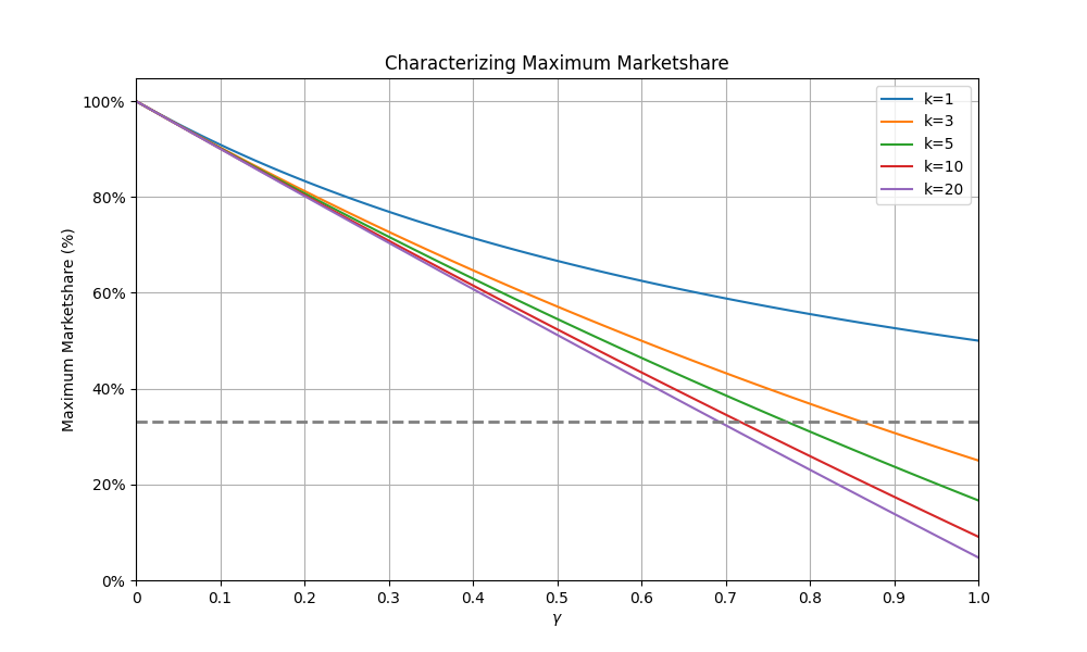
Figure 1: The maximum equilibrium market share of any BP with a BP set that is $(\gamma,k)$-competitive in the sense of Definition 3.2, as characterized by Theorem 3.3. The horizontal dotted line corresponds to a market share of 33%, which is a critical security threshold for many proof-of-stake blockchain protocols.

We next turn to the proof of Theorem 3.3. We require the following monotonicity lemma, which follows from basic properties of separable concave maximization problems (like the one in Proposition 3.1). The details are left to the appendix.

Lemma 3.4 (First Monotonicity Lemma)

For a BP set $I$, base reward $r$, and cost parameter $c$, let $\mu$ and $\mu^{\prime}$ denote two nonnegative reward multiplier vectors that are identical except that, for some $j\in I$, $\mu^{\prime}_{j}>\mu_{j}$. Then, for every $i\neq j$, $\hat{x}_{i}(\mu^{\prime},r,c)\leq\hat{x}_{i}(\mu,r,c)$.

With this lemma in hand, we can now prove Theorem 3.3.

Proof of Theorem 3.3: We begin with part (b). Fix $r>0$, $c>0$, $\gamma\in[0,1]$, and $k\geq 1$. Consider a set of $k+1$ BPs for which $\mu_{1}=1/\gamma$ and $\mu_{2}=\mu_{3}=\cdots=\mu_{k+1}=1$; this set is $(\gamma,k)$-competitive. We proceed to guess and check the equilibrium allocation or, equivalently, the optimal solution to (2)–(4). Set

$$\hat{x}_{1}=1-\gamma\cdot\frac{k}{k+\gamma}$$

and

$$\hat{x}_{i}=\gamma\cdot\frac{1}{k+\gamma}$$

for each $i=2,3,\ldots,k+1$. This allocation is feasible (i.e., satisfies (3) and (4)) and satisfies the optimality conditions in (5) and (6) with $\lambda=k/(k+\gamma)$. It is therefore an equilibrium allocation vector, and the value of $\hat{x}_{1}$ is as claimed.

For part (a), consider an arbitrary $(\gamma,k)$-competitive set of $n$ BPs, with reward multipliers $\mu_{1}\geq\mu_{2}\geq\cdots\geq\mu_{n}=1$. Define alternative reward multipliers $\mu^{\prime}$ as follows: $\mu^{\prime}_{1}=\mu_{1}$, $\mu^{\prime}_{i}=\gamma\cdot\mu_{1}$ for $i=2,3,\ldots,k+1$, and $\mu^{\prime}_{i}=0$ for $i=k+1,k+2,\ldots,n$. Because the given BP set is $(\gamma,k)$-competitive, $\mu^{\prime}_{i}\leq\mu_{i}$ for every $i$. The First Monotonicity Lemma (Lemma 3.4), applied once for each $i=2,3,\ldots,n$, implies that $\hat{x}_{1}(\mu,r,c)\leq\hat{x}_{1}(\mu^{\prime},r,c)$. (That lemma holds for arbitrary nonnegative reward multipliers and does not require that $\mu^{\prime}_{n}=1$.) By the proof of part (b), $\hat{x}_{1}(\mu^{\prime},r,c)=1-(\gamma\cdot k)/(k+\gamma)$. (Additional BPs with $\mu_{i}=0$ do not change the equilibrium allocation.) Thus $\hat{x}_{1}(\mu,r,c)\leq 1-(\gamma\cdot k)/(k+\gamma)$, as required. $\blacksquare$

4 Long-Run Forces Toward Centralization

4.1 The Staking Process

We next extend the basic model of Section 2 in an orthogonal direction, to investigate connections between BP heterogeneity and centralization from a different angle. In contrast to the single-shot setup of Section 3, this section studies the evolution over time of the stakes controlled by different BPs. We assume here that BPs are non-strategic and always stake all of the native currency that they possess (including reinvesting any earned rewards back into staking).

Precisely, we again consider a set $I$ of $n$ BPs with reward multipliers $\mu_{1}\geq\mu_{2}\geq\cdots\geq\mu_{n}=1$ and a base reward $r$. In addition, each BP $i$ has a positive initial stake, denoted $\pi_{i,1}>0$. More generally, $\pi_{i,t}$ will denote the stake controlled by BP $i$ after $t-1$ block production opportunities have passed. We consider the following probabilistic process, which we call the staking process, for $t=1,2,\ldots,$:

• For block production opportunity $t$, one BP is chosen with probability proportional to the current BP stakes. That is, BP $i$ is chosen with probability

  $$x_{i,t}=\frac{\pi_{i,t}}{\sum_{j\in I}\pi_{j,t}}.$$

• If BP $i^{*}$ is chosen for this opportunity, then the stakes evolve according to:

  $$\pi_{i,t+1}=\begin{cases}\pi_{i,t}+\mu_{i}\cdot r,&\text{if}\ i=i^{*}\\ \pi_{i,t}&\text{if}\ i\neq i^{*}.\end{cases}$$

Thinking of $r$ as fixed throughout this section, the staking process is fully described by the reward multiplier vector $\mu=(\mu_{1},\ldots,\mu_{n})$ and the initial stake vector $\pi=(\pi_{1,1},\ldots,\pi_{n,1})$. We generally assume (without loss of generality) that the entries of $\mu$ are sorted in nonincreasing order; we make no assumptions about $\pi$. One advantage of this setup is that it connects directly to the theory of generalized Pólya urn models (e.g., [20]).

We will be interested in the long-run behavior of the staking process (as a function of $\mu$ and $\pi$), and in particular whether it “centralizes” in the sense that a single BP dominates the staking distribution:

Definition 4.1 ($\epsilon$-Centralization)

For a parameter $\epsilon>0$, the staking process is $\epsilon$-centralized at block $t$ if, for some BP $i$,

$$x_{i,t}\geq 1-\epsilon.$$

With this setup and notion of centralization, we now have another concrete way to quantify the extent to which heterogeneity across BPs leads to centralization: as a function of the heterogeneity in the reward multiplier sequence (the $\mu_{i}$’s), how quickly (if at all) does the staking process become $\epsilon$-centralized?

It is natural to conjecture that, if $\mu_{1}>\mu_{2}$ and $t\rightarrow\infty$, the first BP should, with probability 1, end up with all but a vanishingly small fraction of the overall stake (no matter what the initial stake distribution is). (Intuitively, the rate of increase in the first BP’s stake should outpace that of the others.) This conjecture is in fact true, although the proof is not at all obvious (see Janson [17]). Our concern here will be on the speed with which the staking distribution concentrates. The hope is that, provided there is not too much heterogeneity across BPs (e.g., with $\mu_{2}$ close to $\mu_{1}$), stake concentrates slowly, perhaps even slowly enough to not be a first-order concern. Such a quantitative analysis is necessary to assess the potential benefits of any design aimed to reduce BP heterogeneity (and slow down centralization), such as the proposer-builder separation idea described in Section 5.

4.2 Quantifying the Speed of Centralization

We are now primarily interested in defining quantitative lower and upper bounds on how many blocks it takes for the staking process to become $\epsilon$-centralized. For ease of exposition we will refer to the sum of all the BPs’ stakes at block $t$, not including BP 1, by $\pi_{-1,t}=\sum_{j\in I,j\neq 1}\pi_{j,t}$. We omit the subscript on time when referring to the starting stakes, writing $\pi_{1}$ for $\pi_{1,1}$ and $\pi_{-1}$ for $\pi_{-1,1}$.

Theorem 4.2 (Bounds on Number of Blocks for $\epsilon$-Centralization)

Let $\beta=\max\{\frac{\mu_{1}r}{\pi_{1}},\frac{\mu_{2}r}{\pi_{-1}}\}$ and $\rho=\frac{\pi_{-1}}{\pi_{1}}$. Then for every $\epsilon>0$:

1. (Upper bound on time to centralization) For every

   $$t>\frac{3}{2\mu_{2}r}\left(\pi_{1}\left(\frac{3\rho(1-\epsilon)}{\epsilon}\right)^{\frac{\mu_{1}}{\mu_{1}-\mu_{2}}}+\pi_{-1}\left(\frac{3\rho(1-\epsilon)}{\epsilon}\right)^{\frac{\mu_{2}}{\mu_{1}-\mu_{2}}}\right),$$

   we have

   $$\Pr\left(x_{1,t}<1-\epsilon\right)<8\beta.$$

2. (Lower bound on time to centralization) For every

   $$t<\frac{1}{2\mu_{1}r}\left(\pi_{1}\left(\frac{\rho(1-\epsilon)}{3\epsilon}\right)^{\frac{\mu_{1}}{\mu_{1}-\mu_{n}}}+\pi_{-1}\left(\frac{\rho(1-\epsilon)}{3\epsilon}\right)^{\frac{\mu_{n}}{\mu_{1}-\mu_{n}}}-2(\pi_{1}+\pi_{-1})\right),$$

   we have

   $$\Pr\left(x_{1,t}\geq 1-\epsilon\right)<8\beta.$$

The proof of Theorem 4.2 can be found in the Appendix. Observe that the parameter $\beta$ that controls the probability bounds is small provided the rewards earned by BPs are small relative to their initial stakes. We can see that the dominating factor in the speed to $\epsilon$-centralization is the difference between $\mu_{1}$ and $\mu_{2}$. Reducing this gap causes an exponential increase in the time it takes for the process to $\epsilon$-centralize. As a concrete example, suppose that BP 1 begins with 10% of the stake and we consider the time required for it to control at least 33% of the stake. This corresponds to the parameter values $\rho=9$ and $\epsilon=2/3$. In this case, decreasing $\mu_{1}-\mu_{2}$ from $0.5$ to $0.1$ can increase the number of blocks needed to $\epsilon$-centralize by roughly five orders of magnitude. Echoing the economic analysis in Section 3, the probabilistic analysis in this section underscores the importance of mechanisms for eliminating large differences between the reward multipliers of different BPs.

5 Proposer-Builder Separation and BP Heterogeneity

5.1 Idealized Proposer-Builder Separation

Sections 3 and 4 take very different paths to arrive at a similar conclusion: significant BP heterogeneity leads to concentration of stake (at equilibrium with endogenous staking, or in the long run with automatic reinvestment) and, conversely, decentralization can largely survive a small amount of BP heterogeneity. But, in practice, why wouldn’t there be a large amount of BP heterogeneity? As discussed in Section 1, such heterogeneity can easily arise from many sources, such as exclusive access to certain transactions, proprietary block-building algorithms, or differences in computing resources. In the context of Theorems 3.3 and 4.2, one might expect that the parameters $1/\gamma$ and $\mu_{1}-\mu_{2}$ would, in reality, be quite large.

As discussed in Section 1, proposer-builder separation (PBS) is one approach to reducing the degree of BP heterogeneity. An extremely idealized version of PBS, chosen to indicate the best-case scenario, works as follows:

• Every participant chooses exactly one of two roles: a builder or a proposer.

• Only proposers participate directly in the blockchain protocol as validators (committing stake, proposing blocks, casting votes, etc.).

• For each block production opportunity, each builder sends a block (along with a bid) to the proposer that has been chosen for that opportunity. (A builder’s block should be materially independent of the identity of the proposer.)

• The block proposer proposes the block with the highest bid.

• The block proposal is accepted by the other validators and finalized.

• The winning builder pays its bid to the block proposer.

The key observation is that, under the above assumptions, there is no longer any heterogeneity across proposers—the reward for a block production opportunity is the same (namely, the highest bid submitted by a builder), no matter which proposer is chosen to take advantage of it. This case translates to $\gamma=1$ in Theorem 3.3 (with all proposers committing an equal fraction of stake at equilibrium) and $\mu_{1}=\mu_{n}$ in Theorem 4.2 (with the staking distribution not necessarily concentrating at all), and in these senses is consistent with sustainable decentralization.

There are, of course, many ways that reality could depart from this idealized scenario. Here, we stress-test the implicit assumption in PBS that there is no overlap between the set of builders and the set of proposers. (For example, perhaps a successful block-builder chooses to invest some of its profits into operating a number of validators.) Specifically, we allow proposers to privately engage in block-building on the side, in the hopes of constructing a block even more profitable than the highest bid by one of the specialized builders. At the extreme, if proposers are much better block-builders than the specialized builders, proposer-builder separation achieves nothing and we should expect significant proposer heterogeneity and consequent centralization. The hope, then, would be that the builder ecosystem is sufficiently competitive that proposers can rarely if ever profit from privately constructing their own blocks. We next develop a simple model of a competitive builder ecosystem and formalize the extent to which this hope is in fact correct.

5.2 The Equalizing Effects of Competing Builders

We focus on a fixed block production opportunity and consider a finite set $Y$ of $k$ specialized builders. Each builder $y\in Y$ is capable of building a block that generates for it a nonnegative reward of $r_{y}$. Variations in $r_{y}$ across builders $y$ could stem from different information, different block-building algorithms, different choices of random seeds, and so on. We assume that the $r_{y}$’s are independent draws from a distribution $D_{Y}$—in this sense, the builders in $Y$ are all equally proficient on average (for example, because all the inferior builders have already been competed away). The competitiveness of the builder ecosystem is then most simply measured by its size, $k$.

There is a separate finite set $I$ of proposers. One of these, say $i$, is chosen for the block production opportunity under consideration. The proposer $i$ accepts blocks from builders (along with bids), and optionally also builds its own block. We assume that the proposer is capable of building a block that generates a reward of $r_{i}$ for it, where $r_{i}$ is drawn from a distribution $D_{i}$. We assume that proposers follow what is then the obvious reward-maximizing strategy:

• Accept blocks from builders; let $B^{*}$ denote the submitted block with the highest bid (from the builder to the proposer), and denote this bid by $b^{*}$.

• Privately construct a block $B$ that would generate a reward of $r_{i}\sim D_{i}$ for $i$.

• Propose either the block $B^{*}$ (if $b^{*}>r_{i}$) or $B$ (otherwise), thereby earning a reward of $\max\{b^{*},r_{i}\}$.

Heterogeneity across proposers is captured in this model by the proposer-specific distribution $D_{i}$. Perhaps some proposers do not have the resources or inclination for private block-building, and always accept the best block submitted by a builder (so in effect, $D_{i}$ is a point mass at 0) while others privately compete with the specialized builders. Or perhaps some proposers have access to a larger pool of pending transactions than others. How much variation in expected reward is there across proposers, and how does the answer depend on the competitiveness $k$ of the builder ecosystem?

Some version of the following three assumptions is necessary to prove bounds on the degree of heterogeneity of proposer rewards in this model:

• By publishing a builder-proposed block, the proposer should earn no reward beyond the bid of the winning builder. (Intuitively, the builder should have already extracted all of the value of the block it proposed.) If this assumption does not hold, different proposers may earn rewards at much different rates even when they all follow the strategy (S1)–(S3).

• Proposers cannot be significantly better block-builders than the builders in $Y$. (If they are, the builder ecosystem doesn’t matter.) Formally, we will assume that every proposer distribution $D_{i}$ is first-order stochastically dominated (FOSD) by the builder distribution $D_{Y}$. (I.e., for all $x\geq 0$, $\text{\bf Pr}_{r\sim D_{i}}\!\left[r\geq x\right]\leq\text{\bf Pr}_{r\sim D_{Y}}\!\left[r\geq x\right]$.)

• Proposer distributions $D_{i}$ cannot be excessively heavy-tailed. (Otherwise, a proposer with such a distribution could earn vastly more rewards in expectation than a proposer that does no private block-building, even though it is almost never able to outperform the specialized block-builders. For example, this is true if $D_{i}$ is the “equal-revenue distribution,” with distribution function $1-\tfrac{1}{x}$ on $[1,\infty)$.) Formally, we will assume that the builder distribution $D_{Y}$ (which FOSD every proposer distribution $D_{i}$) satisfies the monotone hazard rate (MHR) condition, meaning that $f(x)/(1-F(x))$ is nondecreasing, where $f$ and $F$ denote the PDF and CDF of the distribution. Intuitively, the tails of an MHR distribution are no heavier than those of an exponential distribution.

The main result of this section shows that, under assumptions (A1)–(A3), a competitive builder ecosystem ensures minimal proposer heterogeneity.

Theorem 5.1 (Competition Reduces Proposer Heterogeneity)

Let $Y$ denote a set of $k$ specialized builders, with rewards $r_{y}$ drawn i.i.d. from a distribution $D_{Y}$ that satisfies the MHR condition, and assume that builders bid according to the (unique) Bayes-Nash equilibrium of a symmetric first-price auction with value distribution $D_{Y}$. Let $I$ denote a set of proposers, with proposer $i$’s private block-building reward $r_{i}$ drawn from a distribution $D_{i}$ that is FOSD by $D_{Y}$. Assume that every proposer follows the strategy in (S1)–(S3). Then, for every pair $i,j\in I$ of proposers, the expected reward earned by $i$ (conditioned on selection) is at most

$$1+O\left(\frac{1}{\log k}\right)$$

times that earned by $j$ (conditioned on selection).

Thus, as the competitiveness $k$ of the builder ecosystem increases, the ratio in expected proposer rewards (roughly corresponding to the parameter $\gamma$ in Theorem 3.3 or $\mu_{1}$ in Theorem 4.2) tends to 1.

Proof of Theorem 5.1: The minimum expected reward (conditioned on selection) would be earned by a proposer that never engages in private block-building (equivalently, $D_{i}$ is a point mass at 0). The expected reward of such a proposer would be the expected highest bid by a builder. It is known that, at the unique Bayes-Nash equilibrium of a first-price auction with i.i.d. private valuations (i.e., $r_{i}$’s) and $k$ bidders, the expected highest bid is the expected second-largest sample of $k$ i.i.d. samples from the value distribution (i.e., from $D_{Y}$); see e.g. [19, Proposition 2.3]. Call this quantity $R$. How much bigger could the expected reward (conditioned on selection) of a different proposer be?

Fix a proposer $i$ with reward distribution $D_{i}$ that is FOSD by $D_{Y}$. In the notation of the strategy (S1)-(S3), the expected reward of this proposer (conditioned on selection) is the expected value of $\max\{b^{*},r_{i}\}$. Because builders will, at equilibrium, bid at most their values in a first-price auction, this expected reward can be bounded above by the expectation of $\max\{\max_{y\in Y}r_{y},r_{i}\}$—the expected maximum out of $k$ i.i.d. samples from $D_{Y}$ and one independent sample from $D_{i}$. Because $D_{Y}$ FOSD $D_{i}$, this quantity can, in turn, be bounded above by the expected maximum of $k+1$ i.i.d. samples from $D_{Y}$.

Next, we use the fact that, because $D_{Y}$ satisfies the MHR condition, the expectation of the second-largest value out of $n\geq 2$ i.i.d. samples from $D_{Y}$ is a concave function of $n$ (see [27, Theorem 1(b)]). Because this quantity is also nonnegative and nondecreasing in $n$, this fact implies that the expected second-largest value of $k+1$ i.i.d. samples from $D_{Y}$ is at most $1+\tfrac{1}{k-1}$ times the expected second-largest value of $k$ i.i.d. samples from $D_{Y}$ (i.e., at most $(1+\tfrac{1}{k-1})R$).

It remains to bound the factor by which the expected value of the largest of $k+1$ i.i.d. samples from $D_{Y}$ exceeds that of the second-largest. Using the representation

$$F(x)=1-\exp\left\{-\int_{0}^{x}h(x)dx\right\}$$

of a distribution function $F$ with density $f$, where $h(x)=f(x)/(1-F(x))$ denotes its hazard rate, it follows that this factor is maximized among MHR distributions (those with $h$ nondecreasing) by exponential distributions (those with $h$ constant). A calculation then shows that this factor is at most

$$\frac{\sum_{j=1}^{k+1}\tfrac{1}{j}}{\sum_{j=2}^{k+1}\tfrac{1}{j}}=1+O\left(\frac{1}{\log k}\right).$$

This completes the proof: the expected reward (conditioned on selection) of the proposer $i$ is at most the expected value of $\max\{\max_{y\in Y}r_{y},v_{i}\}$, which is at most the expected value of the largest of $k+1$ i.i.d. samples from $D_{Y}$, which is at most $1+O(1/\log k)$ times the expected value of the second-largest of $k+1$ i.i.d. samples from $D_{Y}$, which is at most $(1+1/(k-1))(1+O(1/\log k))=1+O(1/\log k)$ times $R$ (i.e., the expected second-largest of $k$ i.i.d. samples from $D_{Y}$). $\blacksquare$

Acknowledgments

We thank Justin Drake, Ben Fisch, Mike Neuder, Matt Weinberg, and the FC reviewers for useful comments on a preliminary version of this paper.

Appendix A Proof of Lemma 3.4

Proof.

The optimality conditions for the concave optimization problem in Proposition 3.1 state that optimal solutions are those that are feasible and that equalize the partial derivatives of the objective function (except for unused variables, for which the partial derivative may be lower). That is, a feasible allocation $\mathbf{x}$ is optimal for (2)–(4) if and only if there is a constant $\lambda$ such that

$$\frac{\partial\Phi_{i}}{\partial x_{i}}(\mathbf{x})=\mu_{i}\cdot\frac{r}{c}\cdot(1-x_{i})\leq\lambda$$ (5)

for all $i\in I$ and

$$\frac{\partial\Phi_{i}}{\partial x_{i}}(\mathbf{x})=\mu_{i}\cdot\frac{r}{c}\cdot(1-x_{i})=\lambda$$ (6)

for all $i$ with $x_{i}>0$, where $\Phi_{i}$ denotes the $i$th term of the objective function in (2). Starting from the allocation $\hat{\mathbf{x}}(\mu,r,c)$ (with constant $\lambda$), increasing $\mu_{j}$ increases $\partial\Phi_{j}/\partial x_{j}$. If its new value remains at most $\lambda$, then the equilibrium allocation remains the same. If its new value exceeds $\lambda$, to compensate and restore the optimality conditions, $x_{j}$ must increase and every other $x_{i}$ (that is not already 0) must decrease. ∎

Appendix B Proof of Theorem 4.2

B.1 Proof of Upper Bound

We start with a monotonicty lemma that shows increasing how competitive the block producers are can only increase the number of blocks it takes for centralization to occur. This is intuitive since if BP 1’s competitors start earning more, the rate at which BP 1 accrues their advantage becomes slower. We will use this to show that if $\mu^{\prime}$ is more competitive than $\mu,$ then an upper bound on the number of blocks till $\epsilon$-centralization for $\mu^{\prime}$ also holds for $\mu$.

Lemma B.1 (Second Monotonicity Lemma)

Let $\mu$ and $\mu^{\prime}$ be two block producer sets with initial starting stakes $\pi$ where $\mu_{i}^{\prime}\geq\max_{i\in I,i\neq 1}\{\mu_{i}\}$ for all $i\geq 2$. Then $\Pr(x_{1,t}>a)\geq\Pr(x^{\prime}_{1,t}>a)$ for all $a\in[0,1]$ where $x_{1,t}$ and $x^{\prime}_{1,t}$ correspond to BP 1’s chance of being chosen at block $t$ under $(\mu,\pi)$ and $(\mu^{\prime},\pi)$ respectively.

Proof.

Here we give a formal proof of the coupling argument sketched in the main body. Let $\Pi=(\pi_{t})_{t\geq 1}$ and $\Pi^{\prime}=(\pi^{\prime}_{t})_{t\geq 1}$ be the staking processes under $\mu$ and $\mu^{\prime}$ respectively, both with starting stakes $\pi$. Then consider the following coupling for $(\Pi,\Pi^{\prime})$.

For all blocks $t$: Define $a_{0,t}=a^{\prime}_{0,t}=0$. Then for all $i\in I$, recursively define

$$a_{i,t}=x_{i,t}+a_{i-1,t}\text{ and similarly }a^{\prime}_{i,t}=x^{\prime}_{i,t}+a^{\prime}_{i-1,t}$$

Then consider the following process to choose the block producer for every block $t$:
(1) Sample $y_{t}\sim U[0,1]$, (2) Let $i^{*}_{t}=i$ if $y_{t}\in(a_{i-1,t},a_{i,t}]$, (3) Let $i^{\prime*}_{t}=i$ if $y_{t}\in(a_{i-1,t},a_{i,t}]$

Crucially we are using the same randomness to sample the winner under both $\Pi$ and $\Pi^{\prime}$ in every block. Combining this with the fact $a_{i,t}-a_{i-1,t}=x_{i,t}$, $a^{\prime}_{i,t}-a^{\prime}_{i-1,t}=x^{\prime}_{i,t}$ and $y_{t}$ is sampled uniformly random from $[0,1]$ gives us that the marginal distributions of $\Pi$ and $\Pi^{\prime}$ under this coupling match their distributions under the staking process. Thus this process is a valid coupling, and to prove the lemma, it suffices to show that for every sequence of random draws $\{y_{t}\}_{t\geq 1}$ that $x_{1,t}\geq x^{\prime}_{1,t}$. We proceed to show this via strong induction.

The base case follows trivially since both processes start with the same stakes $\pi$ so $x_{1,1}=x^{\prime}_{1,1}$. Now for the inductive hypothesis assume that for all sequences $\{y_{t}\}_{1\leq t\leq k-1}$, $x_{1,s}\geq x^{\prime}_{1,s}$ for all $s=1,...,k$ . We then show that for any $y_{k}\in[0,1]$ that $x_{1,k+1}\geq x^{\prime}_{1,k+1}$.

We start by claiming that $\pi_{1,k}\geq\pi^{\prime}_{1,k}$. This follows from the strong inductive hypothesis since $x_{1,s}\geq x^{\prime}_{1,s}$ for all $s\leq k$ implies that whenever $y_{t}\leq x^{\prime}_{1,t}$ that $y_{t}\leq x_{1,t}$ for all $t\leq k$. Since $\mu_{1}=\mu^{\prime}_{1}$ this gives us $\pi_{1,k}\geq\pi^{\prime}_{1,k}$. Now fix any $y_{k}\in[0,1]$. Then from our inductive hypothesis, we have 3 cases: (1) $y_{k}\leq x^{\prime}_{1,k}\leq x_{1,k}$, (2) $x^{\prime}_{1,k}<y_{k}<x_{1,k}$, or (3) $x^{\prime}_{1,k}<x_{1,k}<y_{k}$. In particular note the case where $i^{*}_{k}\neq 1$ but $i^{\prime*}_{k}=1$ can never happen. We will show that each of these three cases will lead to $x_{1,k+1}\geq x^{\prime}_{1,k+1}$. We use $\Pi_{t}=\sum_{i\in I}\pi_{i,t}$ and $\Pi^{\prime}_{t}=\sum_{i\in I}\pi^{\prime}_{i,t}$ to refer to the total stakes at time $t$ under $\Pi$ and $\Pi^{\prime}$ respectively.

1. $i^{*}_{k}=1,i^{\prime*}_{k}=1$: Here $\frac{\pi_{1,k}}{\Pi_{k}}\geq\frac{\pi^{\prime}_{1,k}}{\Pi^{\prime}_{k}}\implies\frac{\pi_{1,k}+\mu_{1}r}{\Pi_{k}+\mu_{1}r}\geq\frac{\pi^{\prime}_{1,k}+\mu_{1}r}{\Pi^{\prime}_{k}+\mu_{1}r}$

2. $i^{*}_{k}=1,i^{\prime*}_{k}=i\neq 1$: Here $\frac{\pi_{1,k}}{\Pi_{k}}\geq\frac{\pi^{\prime}_{1,k}}{\Pi^{\prime}_{k}}\implies\frac{\pi_{1,k}+\mu_{1}r}{\Pi_{k}+\mu_{1}r}\geq\frac{\pi^{\prime}_{1,k}}{\Pi^{\prime}_{k}+\mu_{i}r}$

3. $i^{*}_{k}=i\neq 1,i^{\prime*}_{k}=j\neq 1$: Here we use $\pi_{1,k}\geq\pi^{\prime}_{1,k}$, $\mu_{i}\leq\mu^{\prime}_{j}$, and $\frac{\pi_{1,k}}{\Pi_{k}}\geq\frac{\pi^{\prime}_{1,k}}{\Pi^{\prime}_{k}}$ to get $\frac{\pi_{1,k}}{\Pi_{k}+\mu_{i}}\geq\frac{\pi^{\prime}_{1,k}}{\Pi^{\prime}_{k}+\mu^{\prime}_{j}}$

Hence in all cases we get $x_{1,k+1}\geq x^{\prime}_{1,k+1}$.

∎

With the monotonicity of the effect of competitiveness on the blocks to centralization established, we are ready to prove the main theorem.

Proof.

We start by proving the upper bound for the staking process $(\mu,\pi)$.

Reducing to Two Block Producers:

We first show that it suffices to prove the upper bound for the case with two block producers where $\hat{\mu}=(\mu_{1},\mu_{2})$ and $\hat{\pi}=(\pi_{1},\pi_{-1})$. To see this, consider $\mu^{\prime}=(\mu_{1},\mu_{2},...,\mu_{2})$ where $\mu^{\prime}_{i}=\mu_{2}$ for $i\geq 2$ with the same starting stakes $\pi$. Since $\mu_{2}=\max_{i\in I,i\neq 1}\{\mu_{i}\}$ , by lemma B.1 we have that the probability $(\mu,\pi)$ is $\epsilon$-centralized at block $t$ first order stochastically dominates the probability $(\mu^{\prime},\pi)$ is $\epsilon$-centralized at block $t$. Furthermore, note that for the purposes of finding an upper bound on the number of blocks it takes for $(\mu^{\prime},\pi)$ to $\epsilon$-centralize, we are only concerned with how fast $\pi^{\prime}_{1,t}$ grows compared to $\pi^{\prime}_{-1,t}$. Then since $\mu^{\prime}_{i}=\mu_{2}$ for all $i\geq 2$, $\pi^{\prime}_{-1,t}$ increases by the same amount if $i^{*}_{t}\neq 1$ regardless of which block producer is chosen. Thus the probability $i^{*}_{t}\neq 1$ for future blocks is also the same regardless of which $i\in I\setminus\{1\}$ is chosen. This implies that the time to $\epsilon$-centralization is equivalent under $(\mu^{\prime},\pi)$ and $(\hat{\mu},\hat{\pi})$. It follows that $\Pr(\hat{x}_{1,t}>a)=\Pr(x^{\prime}_{1,t}>a)\leq\Pr(x_{1,t}>a)$ for all blocks $t\geq 1$ and $a\in[0,1]$, making it sufficient to prove the upper bound holds for $(\hat{\mu},\hat{\pi})$. Thus from here we will assume WLOG that there are only two block producers with $\mu=(\mu_{1},\mu_{2})$ and $\pi=(\pi_{1},\pi_{-1})$

Passing to the Continuous Case:

As has been noted previously, the process describing how stake evolves can be modeled as a Pólya urn with a diagonal replacement matrix. Imagine an urn with all of the staked coins where each coin has a corresponding block producer. Then for every block production opportunity, a coin is randomly sampled from the urn. If the coin is owned by BP $i$, then $\mu_{i}r$ additional coins corresponding to BP $i$ are added to the urn. Analyzing the dynamics of unbalanced urns, where different amounts of coins are added to the urn depending on who is chosen, tends to be difficult in the discrete scheme because the total amount of coins in the urn is dependent on the history of what coins were chosen.

To get around this, a classic technique in studying Pólya urns is embedding the discrete process into a continuous one. In the continuous case, the discrete sampling process is replaced with a birth-death branching process. Every coin in the urn is given a clock with a i.i.d Exp(1) random expiry date. If a coin belonging to BP $i$ expires, that coin’s clock resets and $\mu_{i}r$ new coins belonging to BP $i$ are added to the urn, each also with their own i.i.d. Exp(1) clocks. Since the Exp(1) distribution is memoryless, it follows that at any given time, the next clock to go off will be uniformly sampled from all of the coins in the urn. Thus the probability the next coin chosen is BP $i$’s matches the probability they would have been selected in the discrete process. Thus, if we consider snapshots of the continuous process at the times the clocks expire, then this process is distributed identically to the discrete process. This lets us prove results about the staking process by proving results in the continuous version of the staking process and then inverting back to the discrete case.

The primary advantage of working in the continuous case is that coins from different BPs don’t affect each other. Notice that a clock expiring for one BP’s coins have no influence on how another BP’s coins evolve. We can make this precise by observing that each BP’s coins grow according to independent Yule processes. Since we have shown it suffices to consider the case with two block producers, we will have two processes $\Pi_{1}(t)$ and $\Pi_{2}(t)$ representing the evolution of stake for $\pi_{1,t}$ and $\pi_{2,t}$ respectively. The fact that $\Pi_{1}(t)$ and $\Pi_{2}(t)$ evolve independently, lets us bound the ratio of $\Pi_{1}(t)/\Pi_{2}(t)$ via concentration bounds on $\Pi_{1}(t)$ and $\Pi_{2}(t)$ independently. From [20] we have that E$[\Pi_{1}(t)]=\pi_{1}e^{\mu_{1}rt}$ and Var$[\Pi_{1}(t)]=\mu_{1}r\pi_{1}(e^{2\mu_{1}r}-\mu_{1}rte^{\mu_{1}rt})\leq\mu_{1}r\pi_{1}e^{2\mu_{1}rt}$. Thus we can apply Chebyshev’s inequality to get

$$\Pr\left(|\Pi_{1}(t)-E[\Pi_{1}(t)]|\geq\frac{1}{2}E[\Pi_{1}(t)]\right)\leq\frac{4Var[\Pi_{1}(t)]}{E[\Pi_{1}(t)]^{2}}$$

$$\implies\Pr\left(\Pi_{1}(t)<\frac{1}{2}E[\Pi_{1}(t)]\right)\leq\frac{4\mu_{1}r\pi_{1}e^{2\mu_{1}rt}}{\pi^{2}_{1}e^{2\mu_{1}rt}}=\frac{4\mu_{1}r}{\pi_{1}}$$

The same derivation for BP 2 gives

$$\Pr\left(\Pi_{2}(t)\geq\frac{3}{2}E[\Pi_{2}(t)]\right)\leq\frac{4\mu_{2}r}{\pi_{-1}}.$$

Then using a union bound gives

$$\Pr\left(\frac{\Pi_{1}(t)}{\Pi_{2}(t)}<\frac{\frac{1}{2}E[\Pi_{1}(t)]}{\frac{3}{2}E[\Pi_{2}(t)]}\right)<4r\left(\frac{\mu_{1}}{\pi_{1}}+\frac{\mu_{2}}{\pi_{-1}}\right)$$

Now let $\hat{t}=\frac{\ln\frac{3\pi_{-1}}{\pi_{1}}\frac{1-\epsilon}{\epsilon}}{r(\mu_{1}-\mu_{2})}$. This gives us

$$E[\Pi_{1}(\hat{t})]=\pi_{1}\left(\frac{3\pi_{-1}(1-\epsilon)}{\pi_{1}\epsilon}\right)^{\frac{\mu_{1}}{\mu_{1}-\mu_{2}}}\text{ and }E[\Pi_{2}(\hat{t})]=\pi_{-1}\left(\frac{3\pi_{-1}(1-\epsilon)}{\pi_{1}\epsilon}\right)^{\frac{\mu_{2}}{\mu_{1}-\mu_{2}}}$$

Plugging this into our union bound above gives for any $t\geq\hat{t}$,

$$\Pr\left(\frac{\Pi_{1}(\hat{t})}{\Pi_{2}(\hat{t})}<\frac{1-\epsilon}{\epsilon}\right)\leq 4r\left(\frac{\mu_{1}}{\pi_{1}}+\frac{\mu_{2}}{\pi_{-1}}\right)$$

where $\frac{\Pi_{1}(\hat{t})}{\Pi_{2}(\hat{t})}<\frac{1-\epsilon}{\epsilon}\Leftrightarrow\frac{\Pi_{1}(\hat{t})}{\Pi_{1}(\hat{t})+\Pi_{2}(\hat{t})}<1-\epsilon$

Moving Back to the Discrete Case:

Now that we have shown a $\hat{t}$ for which the continuous process $\epsilon$-centralizes with constant probability, it remains to find how many blocks in the discrete process this corresponds to. Recall every time a clock expires in the continuous process, a block passes in the discrete process. Thus to get an upper bound on how many blocks have passed by time $\hat{t}$, it suffices to upper bound how many clocks are expected to expire by time $\hat{t}$. Observe that the number of coins must increase by at least $\mu_{2}r$ everytime a clock goes off. So if we have an upper bound of the total amount of coins there are at time $\hat{t}$, we know the maximum number of clocks that could have expired. Using this gives an upper bound of $\frac{\Pi_{1}(\hat{t})+\Pi_{2}(\hat{t})}{\mu_{2}r}$ blocks.

Since Chebyshev’s inequality is two-sided, with our union bound from before, we have already accounted for the probability that both $\Pi_{1}(\hat{t})$ and $\Pi_{2}(\hat{t})$ are above $3/2$ their expectations. Hence we can use this bound without suffering any loss to our probability, giving us a bound of

$$\frac{\frac{3}{2}(E[\Pi_{1}(\hat{t})]+E[\Pi_{2}(\hat{t})])}{\mu_{2}r}=\frac{3}{2\mu_{2}r}\left(\pi_{1}\left(\frac{3\pi_{-1}(1-\epsilon)}{\pi_{1}\epsilon}\right)^{\frac{\mu_{1}}{\mu_{1}-\mu_{2}}}\right.+\left.\pi_{-1}\left(\frac{3\pi_{-1}(1-\epsilon)}{\pi_{1}\epsilon}\right)^{\frac{\mu_{2}}{\mu_{1}-\mu_{2}}}\right)$$

Putting it all together, due to the equivalence of the continuous process and the discrete process this gives us for $t$ greater than this bound that

$$\Pr\left(\frac{\pi_{1,t}}{\pi_{1,t}+\pi_{-1,t}}<1-\epsilon\right)<4r\left(\frac{\mu_{1}}{\pi_{1}}+\frac{\mu_{2}}{\pi_{-1}}\right)<8\beta$$

.
∎

B.2 Proof of Lower Bound

Here we go through the proof of the lower bound in Theorem 4.2 for a staking process $(\mu,\pi)$. We largely elide the exposition justifying steps that are directly mirrored in the upper bound.

We start with a corollary of lemma B.1 that gives us a monotonicity result in the other direction. If we decrease the competitiveness of the BPs apart from BP 1, then the time to centralization can only decrease. Similarly to the previous lemma, we will use this to show that if $\mu^{\prime}$ is less competitive than $\mu$, then a lower bound for the number of blocks till $\epsilon$-centralization for $\mu^{\prime}$ also holds for $\mu$.

Corollary B.2

Let $\mu$ and $\mu^{\prime}$ be two block producer sets with initial starting stakes $\pi$ where $\mu^{\prime}_{i}\leq\min_{i\in I}\{\mu_{i}\}$ for all $i\geq 2$. Then $\Pr(x_{1,t}<a)\geq\Pr(x^{\prime}_{1,t}<a)$ for all $a\in[0,1]$ where $x_{1,t}$ and $x^{\prime}_{1,t}$ correspond to BP 1’s chance of being chosen at block $t$ under $(\mu,\pi)$ and $(\mu^{\prime},\pi)$ respectively.

Proof.

From how $\mu^{\prime}$ is defined we have that $\mu_{i}\geq\max_{i\in I,i\neq 1}\{\mu^{\prime}_{i}\}$. Thus by lemma B.1 we have that $\Pr(x^{\prime}_{1,t}>a)\geq\Pr(x_{1,t}>a)$ implying $\Pr(x_{1,t}<a)\geq\Pr(x^{\prime}_{1,t}<a)$. ∎

With this monotonocity result we can continue with the proof of the lower bound.

Proof.

We start by reducing our analysis to the case of two block producers. Let $\mu^{\prime}=(\mu_{1},\mu_{n},...,\mu_{n})$. Then since $\mu_{n}=\min_{i\in I}\{\mu_{i}\}$ we can apply Corollary B.2 to get that a lower bound for $(\mu^{\prime},\pi)$ also holds for $(\mu,\pi)$. Then, like in the upper bound, we note that $\mu_{i}=\mu_{j}$ for all $i,j\neq 1$ implies that $(\mu^{\prime},\pi)$ $\epsilon$-centralizes at the same rate as the process $((\mu_{1},\mu_{n}),(\pi_{1},\pi_{-1})$. Thus WLOG we continue by letting $\mu=(\mu_{1},\mu_{n})$ and $\pi=\pi_{1},\pi_{-1}$.

Now we move to the continuous case, letting $\Pi_{1}(t)$ and $\Pi_{2}(t)$ represent the evolution of $\pi_{1,t}$ and $\pi_{-1,t}$ respectively. Note these are the same yule processes we had in the upper bound with the slight modification of changing $\mu_{2}$ to $\mu_{n}$ in $\Pi(2)$. Thus we can use Chebyshev again to get

$$\Pr\left(\Pi_{1}(t)>\frac{3}{2}E[\Pi_{1}(t)]\right)<\frac{4\mu_{1}r}{\pi_{1}}\text{ and }\Pr\left(\Pi_{2}(t)<\frac{1}{2}E[\Pi_{2}(t)]\right)<\frac{4\mu_{n}r}{\pi_{-1}}$$

A union bound then gives

$$\Pr\left(\frac{\Pi_{1}(t)}{\Pi_{2}(t)}>\frac{\frac{3}{2}E[\Pi_{1}(t)]}{\frac{1}{2}E[\Pi_{2}(t)]}\right)<4r\left(\frac{\mu_{1}}{\pi}+\frac{\mu_{n}}{\pi_{-1}}\right)$$

We can then let $\hat{t}=\frac{\ln\frac{\pi_{-1}}{3\pi_{1}}\frac{(1-\epsilon}{\epsilon})}{r(\mu_{1}-\mu_{n})}$ giving us

$$E[\Pi_{1}(\hat{t})]=\pi_{1}\left(\frac{\pi_{-1}(1-\epsilon)}{3\pi_{1}\epsilon}\right)^{\frac{\mu_{1}}{\mu_{1}-\mu_{n}}}\text{ and }E[\Pi_{2}(\hat{t})]=\pi_{-1}\left(\frac{\pi_{-1}(1-\epsilon)}{3\pi_{1}\epsilon}\right)^{\frac{\mu_{n}}{\mu_{1}-\mu_{n}}}$$

Plugging $\hat{t}$ into the union bound then gives

$$\Pr\left(\frac{\Pi_{1}(\hat{t})}{\Pi_{2}(\hat{t})}\geq\frac{1-\epsilon}{\epsilon}\right)\leq 4r\left(\frac{\mu_{1}}{\pi_{1}}+\frac{\mu_{n}}{\pi_{-1}}\right)$$

.

Now all that remains is to convert back to a bound in the discrete case. Here we want a lower bound on the total amount of stake that the continuous process adds by time $\hat{t}$. Combining this with the fact that the maximum the total stake increases in any block is $\mu_{1}$ gives us a lower bound on how many blocks need to pass before the staking process can centralize. One difference in the analysis here between the upper and lower bound is that we also need to subtract the starting stake amounts on the bound for the total stake at time $\hat{t}$ to get a lower bound on how much stake was added.

Again like the upper bound, because Chebyshev is two-sided we have already paid for the probability bounding the probability $\Pi_{1}(t)$ and $\Pi_{2}(t)$ are below half their expectations. Thus without losing any more probability we can get a bound of

$$\Pi_{1}(\hat{t})+\Pi_{2}(\hat{t})<\frac{1}{2}\left(E[\Pi_{1}(\hat{t})]+E[\Pi_{2}(\hat{t})]\right)=\frac{1}{2}\left(\pi_{1}\left(\frac{\rho(1-\epsilon)}{3\epsilon}\right)^{\frac{\mu_{1}}{\mu_{1}-\mu_{n}}}+\pi_{-1}\left(\frac{\rho(1-\epsilon)}{3\epsilon}\right)^{\frac{\mu_{n}}{\mu_{1}-\mu_{n}}}\right)$$

Putting everything together gives a lower bound of

$$\frac{\frac{1}{2}E[\Pi_{1}(\hat{t})+\Pi_{2}(\hat{t})]-\Pi_{1}(0)-\Pi_{2}(0)}{\mu_{1}r}>\frac{1}{2\mu_{1}r}\left(\pi_{1}\left(\frac{\rho(1-\epsilon)}{3\epsilon}\right)^{\frac{\mu_{1}}{\mu_{1}-\mu_{n}}}+\pi_{-1}\left(\frac{\rho(1-\epsilon)}{3\epsilon}\right)^{\frac{\mu_{n}}{\mu_{1}-\mu_{n}}}-2(\pi_{1}+\pi_{-1})\right)$$

where for $t$ less than this bound,

$$\Pr(x_{1,t}\geq 1-\epsilon)<4r\left(\frac{\mu_{1}}{\pi}+\frac{\mu_{n}}{\pi_{-1}}\right)<8\beta$$

∎

References

- [1] Alsabah, H., Capponi, A.: Pitfalls of bitcoin’s proof-of-work: R&d arms race and mining centralization. Available at SSRN 3273982 (2020)
- [2] Arnosti, N., Weinberg, S.M.: Bitcoin: A natural oligopoly. Manag. Sci. 68(7), 4755–4771 (2022)
- [3] Athreya, K.B., Karlin, S.: Embedding of urn schemes into continuous time markov branching processes and related limit theorems. The Annals of Mathematical Statistics 39(6), 1801–1817 (1968)
- [4] Bahrani, M., Garimidi, P., Roughgarden, T.: Transaction fee mechanism design with active block producers. CoRR abs/2307.01686 (2023)
- [5] Buchanan, J.M., Tollison, R.D., Tullock, G.: Toward a theory of the rent-seeking society. Texas A&M University economics series, Texas A & M University (1980)
- [6] Budish, E.: The economic limits of bitcoin and the blockchain. Working Paper 24717, National Bureau of Economic Research (June 2018)
- [7] Buterin, V.: Endgame (2021), https://vitalik.ca/general/2021/12/06/endgame.html
- [8] Buterin, V.: Proposer/block builder separation-friendly fee market designs (2021), https://ethresear.ch/t/proposer-block-builder-separation-friendly-fee-market-designs/9725
- [9] Dimitri, N.: Bitcoin mining as a contest. Ledger 2, 31–37 (2017)
- [10] Eggenberger, F., Pólya, G.: Über die statistik verketteter vorgänge. ZAMM - Journal of Applied Mathematics and Mechanics / Zeitschrift für Angewandte Mathematik und Mechanik 3(4), 279–289 (1923). https://doi.org/https://doi.org/10.1002/zamm.19230030407, https://onlinelibrary.wiley.com/doi/abs/10.1002/zamm.19230030407
- [11] Fanti, G., Kogan, L., Oh, S., Ruan, K., Viswanath, P., Wang, G.: Compounding of wealth in proof-of-stake cryptocurrencies. In: Goldberg, I., Moore, T. (eds.) Financial Cryptography and Data Security - 23rd International Conference, FC 2019, Frigate Bay, St. Kitts and Nevis, February 18-22, 2019, Revised Selected Papers. Lecture Notes in Computer Science, vol. 11598, pp. 42–61. Springer (2019)
- [12] Flashbots: Mev-boost in a nutshell (2023), https://boost.flashbots.net/
- [13] Gradstein, M.: Intensity of competition, entry and entry deterrence in rent seeking contests. Economics & Politics 7(1), 79–91 (1995)
- [14] Gupta, T., Pai, M.M., Resnick, M.: The centralizing effects of private order flow on proposer-builder separation. In: Bonneau, J., Weinberg, S.M. (eds.) 5th Conference on Advances in Financial Technologies, AFT 2023, October 23-25, 2023, Princeton, NJ, USA. LIPIcs, vol. 282, pp. 20:1–20:15. Schloss Dagstuhl - Leibniz-Zentrum für Informatik (2023)
- [15] Hillman, A.L., Riley, J.G.: Politically contestable rents and transfers. Economics & Politics 1(1), 17–39 (1989)
- [16] Huang, Y., Tang, J., Cong, Q., Lim, A., Xu, J.: Do the rich get richer? fairness analysis for blockchain incentives. In: Li, G., Li, Z., Idreos, S., Srivastava, D. (eds.) SIGMOD ’21: International Conference on Management of Data, Virtual Event, China, June 20-25, 2021. pp. 790–803. ACM (2021)
- [17] Janson, S.: Limit theorems for triangular urn schemes. Probability Theory and Related Fields 134(3), 417–452 (2006)
- [18] Johari, R., Tsitsiklis, J.N.: Efficiency loss in a network resource allocation game. Math. Oper. Res. 29(3), 407–435 (2004)
- [19] Krishna, V.: Auction theory. Academic press (2009)
- [20] Mahmoud, H.: Pólya urn models. CRC press (2008)
- [21] Monderer, D., Shapley, L.S.: Potential games. Games and economic behavior 14(1), 124–143 (1996)
- [22] Rosu, I., Saleh, F.: Evolution of shares in a proof-of-stake cryptocurrency. Manag. Sci. 67(2), 661–672 (2021)
- [23] Roughgarden, T.: Potential functions and the inefficiency of equilibria. In: Proceedings of the International Congress of Mathematicians (ICM). vol. 3, pp. 1071–1094 (2006)
- [24] Tang, W.: Stability of shares in the proof of stake protocol–concentration and phase transitions. arXiv preprint arXiv:2206.02227 (2022)
- [25] Tang, W.: Trading and wealth evolution in the proof of stake protocol. arXiv preprint arXiv:2308.01803 (2023)
- [26] Thiery, T.: Empirical analysis of builders’ behavioral profiles (bpps) (2023), https://ethresear.ch/t/empirical-analysis-of-builders-behavioral-profiles-bbps/16327
- [27] Watt, M.: Concavity and convexity of order statistics in sample size. arXiv preprint arXiv:2111.04702 (2021)