Weak second-order quantum state diffusion unraveling of the Lindblad master equation

Abstract

Simulating mixed-state evolution in open quantum systems is crucial for various chemical physics, quantum optics, and computer science applications. These simulations typically follow the Lindblad master equation dynamics. An alternative approach known as quantum state diffusion unraveling is based on the trajectories of pure states generated by random wave functions, which evolve according to a nonlinear Itô-Schrödinger equation (ISE). This study introduces weak first- and second-order solvers for the ISE based on directly applying the Itô-Taylor expansion with exact derivatives in the interaction picture. We tested the method on free and driven Morse oscillators coupled to a thermal environment and found that both orders allowed practical estimation with a few dozen iterations. The variance was relatively small compared to the linear unraveling and did not grow with time. The second-order solver delivers much higher accuracy and stability with bigger time steps than the first-order scheme, with a small additional workload. However, the second-order algorithm has quadratic complexity with the number of Lindblad operators as opposed to the linear complexity of the first-order algorithm.

I Introduction

When a physical system in a pure quantum state is brought to interact weakly with a macroscopic thermal environment, it changes its energy and chemical composition. At the same time, it gradually loses its "quantumness" or, more technically, its phase coherence. Ultimately, the system’s state resembles that drawn randomly from the Gibbs ensemble at the environment’s temperature and chemical potentials. All quantum systems interact with the environment. Therefore, techniques to simulate decoherence and decay processes are vital for developing quantum technologies and studying chemical processes in solutions and condensed matter. [1, 2, 3, 4, 5, 6, 7, 8, 9, 10, 11, 12, 13, 14, 15, 16, 17]

The pure quantum state of an open system is not known with certainty, and thus, we consider it a random mixture of pure states. The density operator $\rho$ is the mathematical object that best describes this mixture, enabling the calculation of probabilities of outcomes of measurements. Even when the initial mixture $\rho\left(0\right)$ is known, the density operator $\rho\left(t\right)$ changes over time. The Redfield master equation [18, 1, 19, 3, 20, 21] is one way to approximate this, but it sometimes creates mixtures with negative probabilities. Lindblad’s master equation [22, 23, 24, 13, 25] is an augmented form of Redfield’s equation, guaranteeing the density operator’s positivity. It is a quantum Liouville-like equation but includes additional terms, relying on Lindblad operators, to represent the dressed system-environment interactions.

The density operator of the Lindblad equation can be modeled by stochastic processes collectively called "quantum unraveling models." [26, 27, 5] They provide recipes for generating a random time-dependent normalized pure state $\left|\psi\left(t\right)\right\rangle$ for which the expected value of the projector, $\mathbb{E}\left[\left|\psi\left(t\right)\right\rangle\left\langle\psi\left(t\right)\right|\right]$, is identically equal to the Lindblad density operator $\rho\left(t\right)$. One type of unraveling is the Monte-Carlo wave function approach [28, 29, 30], also known as the "quantum jumps model," where the Lindblad operators operate as "jump operators." A second approach to unraveling is the "quantum state diffusion model" [31], involving a norm-conserving (but not unitary) time-dependent stochastic Itô-Schrödinger equation (ISE) for $\left|\psi\left(t\right)\right\rangle$. The ISE contains drift (evolution) and diffusion (fluctuation) terms. The quantum jump and quantum state diffusion models yield different trajectories: the former evolves non-continuously. At the same time, the latter is continuous but non-differentiable in time.

One advantage of basing numerical simulations on the quantum state diffusion model is the availability of well-established high-order techniques for solving stochastic differential equations (SDEs) [5, 32, 33, 34]. In the present contribution, we deploy a simple approach based on exact derivatives in the interaction picture, an Itô-Taylor expansion for weak second-order solutions. The method is stable and allows for high accuracy and slight variance.

II Weak second-order quantum state diffusion unraveling

II.1 Comments on notation

Before we start the detailed theory, here are several comments concerning the notation in this paper:

1. The time dimension of any quantity can be read-off from its superscripts or subscripts: a subscript $0$ adds a dimension of $time^{-1}$ and a superscript $0$ attributes a dimension $time^{+1}$. Thus, the Hamiltonian $\mathcal{H}_{0}$ has the dimension of inverse time while the symbol $I^{0}$ has the dimension of time. A Greek subscript attributes an additional factor of $time^{-1/2}$ and a Greek superscript an additional factor of $time^{1/2}$. Thus, the symbol $I^{\alpha}$ has the dimension of $times^{1/2}$ while $I_{\alpha\beta}$ has the dimension of $time^{-1}.$ The Kronecker-delta $\delta_{\alpha}^{\beta}$ is dimensionless. Furthermore, the symbols $I_{\alpha}^{0}$ and $I_{\gamma}^{\alpha\beta}$ have the dimension of $time^{1/2}$ while $I^{0\alpha}$ has the dimensions of $time^{3/2}$. This convention helps to ascertain that the different time orders we use in our analytical developments are consistent (i.e. that we do not add quantities with different time dimensions).

2. The index $\alpha$, $\alpha^{\prime}$, going from $1,\dots,N_{L}$ denotes one of the $N_{L}$ Lindblad operators. When two quantities indexed with $\alpha$ are multiplied in an expression, a summation over $\alpha$ from 1 to $N_{L}$ is assumed and we omit the explicit $\sum_{\alpha=1}^{N_{L}}$ notation (this is the so-called Einstein convention). If the index is decorated by a dot $\dot{\alpha}$ then no such summation is implied.

3. Below we introduce a “0” operator, in addition to the Lindblad operators. Unlike the $\alpha$, $\alpha^{\prime}$ indices discussed above, going from $1,\dots,N_{L}$, we also use the $\beta$, $\beta^{\prime}$ indices to enumerate operators and quantities that range from $0$ to $N_{L}$. Similar to the case with $\alpha$ , when two quantities indexed with $\beta$ are multiplied in an expression, a summation over $\beta$ is assumed and we omit the explicit $\sum_{\beta=0}^{N_{L}}$ notation. If the index is decorated by a dot $\dot{\beta}$ then no such summation is implied.

II.2 Quantum state diffusion unraveling

The Lindblad equation

$$\dot{\rho}\left(t\right)=-i\left[\mathcal{H}_{0}+\theta\left(t\right)\mathcal{V}_{0},\rho\right]+\mathscr{D}_{0}\rho$$ (1)

together with the initial condition $\rho\left(0\right)$, determines $\rho\left(t\right)$ for all time $t>0$. It contains unitary terms dependent on $\mathcal{H}_{0}$, an effective Hamiltonian operator, and $\theta\left(t\right)\mathcal{V}_{0}$ a driving force with $\theta\left(t\right)$ a dimensionless real time-dependent envelop with time derivative $\theta_{0}\left(t\right)\equiv\dot{\theta}\left(t\right)$. It also contains dissipative terms [31, 24, 25, 13]:

$$\mathscr{D}_{0}\rho \equiv\left[\mathcal{L}_{\alpha}\rho,\mathcal{L}_{\alpha}^{\dagger}\right]+\left[\mathcal{L}_{\alpha},\rho\mathcal{L}_{\alpha}^{\dagger}\right],$$ (2)

defined in terms the Lindblad operators $\mathcal{L}_{\alpha}$, $\alpha=1,\dots,N_{L}$. Atomic units are used ($\hbar=1$, $m_{e}=1$) here, so the energy and inverse time units are identical. Accordingly, $\mathcal{L}_{\alpha}$ have the dimension of $time^{-1/2}$.

Evolving the mixed state density operator $\rho\left(t\right)$ using Eq. (1) can be numerically expensive when systems are large. A possible simplification can be achieved by the unraveling procedure, which evolves a pure random state $\left|\psi\left(t\right)\right\rangle$ in such a way that $\mathbb{E}\left[\left|\psi\left(t\right)\right\rangle\left\langle\psi\left(t\right)\right|\right]=\rho\left(t\right)$. In quantum state diffusion unraveling $\left|\psi\left(t\right)\right\rangle$ is obtained from the following Itô-Schrödinger equation (ISE) [31]

$$\left|d\psi\right\rangle =-i\mathcal{H}_{0}\left|\psi\right\rangle dw^{0}+\Lambda_{\beta}\left|\psi\right\rangle dw^{\beta},$$ (3)

starting from a random ket $\left|\psi\left(0\right)\right\rangle$ for which $\mathbb{E}\left[\left|\psi\left(0\right)\right\rangle\left\langle\psi\left(0\right)\right|\right]=\rho\left(0\right)$. In Eq. (3),

$$\Lambda_{\alpha} \equiv\mathcal{L}_{\alpha}-\left\langle\mathcal{L}_{\alpha}\right\rangle$$

$$\Lambda_{0} \equiv-i\mathcal{\theta}\left(t\right)\mathcal{V}_{0}\left(t\right)+\left(2\left\langle\mathcal{L}_{\alpha}^{\dagger}\right\rangle\mathcal{L}_{\alpha}-\mathcal{L}_{\alpha}^{\dagger}\mathcal{L}_{\alpha}-\left\langle\mathcal{L}_{\alpha}^{\dagger}\right\rangle\left\langle\mathcal{L}_{\alpha}\right\rangle\right),$$

and

$$\left\langle\mathcal{L}_{\alpha}\right\rangle\equiv\frac{\left\langle\psi\left|\mathcal{L}_{\alpha}\right|\psi\right\rangle}{\left\langle\psi\left|\psi\right.\right>}.$$ (4)

Notice that $\left\langle\Lambda_{\alpha}\right\rangle=0$ (for $\alpha=1,\dots,N_{L}$). In the above, $dw^{0}=dt$ is the time-step while $dw^{\alpha}$, $\alpha=1,2,\dots N_{L}$ are independent complex Wiener processes, with real $\Re\left[dw^{\alpha}\right]$ and imaginary $\Im\left[dw^{\alpha}\right]$ parts, each of which is an independent real Wienner process with zero expected value and a variance equal to $dt$. As is common in the stochastic differential equations literature we omit the expected value symbol $\mathbb{E}$ from differentials hence we are lead to the following variances for $dw^{\alpha}$:

$$\left(dw^{\alpha}\right)^{2}=\left(dw^{\alpha*}\right)^{2}=0,\quad\left|dw^{\alpha}\right|^{2}=2dt.$$ (5)

Note that $dw^{\alpha}$ are also independent of $\left|\psi\right\rangle$. Note, that the differential $d\left\langle\psi\left|\psi\right.\right>\equiv\left\langle d\psi\left|\psi\right.\right>+\left\langle\psi\left|d\psi\right.\right>+\left\langle d\psi\left|d\psi\right.\right>$ vanishes when evaluated using Eqs. (3)-(5). Hence $\left\langle\psi\left|\psi\right.\right>$ is a constant of motion, separately for each trajectory.

II.3 Weak first- and second-order propagators

The first step in providing a solution to the ISE, is to move to the interaction picture, defining $\left|\phi\left(t\right)\right\rangle\equiv e^{i\mathcal{H}_{0}t}\left|\psi\left(t\right)\right\rangle$ and for any operator $\mathcal{Y}$, $\mathcal{Y}\left(t\right)\equiv e^{i\mathcal{H}_{0}t}\mathcal{Y}e^{-i\mathcal{H}_{0}t}$. The ISE of Eq. (3) becomes

$$d\left|\phi\right\rangle=dw^{\beta}\Lambda_{\beta}\left(t\right)\left|\phi\right\rangle$$ (6)

where

$$\Lambda_{\alpha}\left(t\right)\equiv\mathcal{L}_{\alpha}\left(t\right)-\left\langle\mathcal{L}_{\alpha}\left(t\right)\right\rangle,$$ (7)

and note our definition of the expectation value

$$\left\langle\mathcal{L}_{\alpha}\left(t\right)\right\rangle\equiv\frac{\left\langle\psi\left(t\right)\left|\mathcal{L}_{\alpha}\right|\psi\left(t\right)\right\rangle}{\left\langle\psi\left(t\right)\left|\psi\left(t\right)\right.\right>}=\frac{\left\langle\phi\left(t\right)\left|\mathcal{L}_{\alpha}\left(t\right)\right|\phi\left(t\right)\right\rangle}{\left\langle\phi\left(t\right)\left|\phi\left(t\right)\right.\right>},$$

which includes division by the norm and thus different from some other applications (e.g., [33]). Formally there is no need to divide by the norm, since one can choose the initial norm as 1 and it is preserved. However, in practice the norm is never perfectly preserved so this division is not a trivial change and we found that division by the norm leads to a more stable numerical behavior.

For developing the numerical scheme, we divide time $t\in\left[0,T_{f}\right]$ where $T_{f}$ is the final time, into $N_{T}$ discrete small temporal segments $\Delta T=T_{f}/N_{T}$, and designate $t_{n+1}=t_{0}+n\Delta T$, $n=1,2,\dots,N_{T}$. Using the notation $\left|\Phi\right\rangle\equiv\left|\phi\left(t_{n}\right)\right\rangle$, the change in the evolving ket during the $n$th time step, $\left|\Delta\Phi\right\rangle\equiv\left|\phi\left(t_{n+1}\right)\right\rangle-\left|\Phi\right\rangle$, is expressed as a stochastic integral over $d\left|\phi\right\rangle$, which gives, using Eq. (6):

$$\left|\Delta\Phi\right\rangle =\int_{t_{n}}^{t_{n}+\Delta T}\Lambda_{\beta}\left(\tau\right)\left|\phi\left(\tau\right)\right\rangle dw_{\tau}^{\beta}.$$ (8)

We strive for an approximation of this integral, which allows an exact solution of the ISE in the limit of $N_{T}\to\infty$ and, accordingly, $\Delta T\to 0$. Our analysis follows closely that found in the classical literature on numerical solutions of real SDEs [35, 36]. Our contribution is the adaptation of the theory to Eq. 6, including the use of complex Wiener processes and exact analytical derivatives therein. We also contribute a simplified notation scheme.

The change in the wave function is provided in terms of first- and second-order contributions, $\left|\Delta\Phi\right\rangle\approx\left|\Delta^{\left(1\right)}\Phi\right\rangle+\left|\Delta^{\left(2\right)}\Phi\right\rangle$. The first-order term is obtained by approximating $\Lambda_{\beta}\left(\tau\right)\left|\phi\left(\tau\right)\right\rangle$ as $\left|\beta\right\rangle\equiv\Lambda_{\beta}\left(t_{n}\right)\left|\Phi\right\rangle$ for $\tau\in\left[t_{n},t_{n}+\Delta T\right]$. This gives:

$$\left|\Delta^{\left(1\right)}\Phi\right\rangle=I^{\beta}\left|\beta\right\rangle,$$ (9)

where $I^{\alpha}=\int_{t_{n}}^{t_{n}+\Delta T}dw^{\alpha}$, $\alpha=1,\dots,N_{L}$ are Itï¿œ integrals given in Table (1) and $I^{0}=\Delta T$. In the numerical calculations we use the model for the complex stochastic Itï¿œ integrals given in the last column of the table.

We use the Itￜ-Taylor expansion to the lowest order for the second-order correction. For this, we introduce a notation in which all quantities are first written as functions of a ket $\left|x\right\rangle$ and a (different) bra $\left\langle y\right|$, then we take separate derivatives with respect to them, and only after that do we set $\left|x\right\rangle=\left|\Phi\right\rangle$ and $\left\langle y\right|=\left\langle\Phi\right|$. In the supplementary information we give a detailed explanation of the results we present here. We define, for $\alpha=1,\dots,N_{L}$ the $\ell$-functions of $\left|x\right\rangle$, $\left\langle y\right|$ and the time $t$,

$$\ell_{\alpha}\left(\left|x\right\rangle,\left\langle y\right|,t\right)\equiv\frac{\left\langle y\left|\mathcal{L}_{\alpha}\left(t\right)\right|x\right\rangle}{\left\langle y\left|x\right.\right>},$$

and

$$\ell_{\alpha}^{*}\left(\left|x\right\rangle,\left\langle y\right|,t\right)\equiv\frac{\left\langle y\left|\mathcal{L}_{\alpha}^{\dagger}\left(t\right)\right|x\right\rangle}{\left\langle y\left|x\right.\right>},$$

which, when evaluated at $\Phi$, become the expectation values of the Lindblad operators:

$$\left(\ell_{\alpha}\left(\left|x\right\rangle,\left\langle y\right|,t\right)\right)_{\Phi} \equiv\ell_{\alpha}\left(\left|\Phi\right\rangle,\left\langle\Phi\right|,t\right)=\left\langle\mathcal{L}_{\alpha}\left(t\right)\right\rangle,$$

$$\left(\ell_{\alpha}^{*}\left(\left|x\right\rangle,\left\langle y\right|,t\right)\right)_{\Phi} \equiv\ell_{\alpha}^{*}\left(\left|\Phi\right\rangle,\left\langle\Phi\right|,t\right)=\left\langle\mathcal{L}_{\alpha}^{\dagger}\left(t\right)\right\rangle.$$

The derivative of $\ell_{\alpha}\left(\left|x\right\rangle,\left\langle y\right|,t\right)$ with respect to the bra $\left\langle y\right|$results in a ket:

$$\left|\frac{\partial}{\partial\left\langle y\right|}\ell_{\alpha}\left(\left|x\right\rangle,\left\langle y\right|,t\right)\right\rangle =\frac{\left(\mathcal{L}_{\alpha}\left(t\right)-\ell_{\alpha}\left(\left|x\right\rangle,\left\langle y\right|,t\right)\right)\left|x\right\rangle}{\left\langle y\left|x\right.\right>}$$

$$\equiv\frac{\left|\lambda_{\alpha}\left(\left|x\right\rangle,\left\langle y\right|,t\right)\right\rangle}{\left\langle y\left|x\right.\right>},$$ (10)

which is orthogonal to $\left|y\right\rangle$:

$$\left\langle y\left|\lambda_{\alpha}\right.\right>=0.$$

Similarly, the derivative with respect to the ket $\left|x\right\rangle$ results in the bra:

$$\left\langle\frac{\partial}{\partial\left|x\right\rangle}\ell_{\alpha}\left(\left|x\right\rangle,\left\langle y\right|,t\right)\right| =\frac{\left\langle y\right|\left(\mathcal{L}_{\alpha}\left(t\right)-\ell_{\alpha}\left(\left|x\right\rangle,\left\langle y\right|,t\right)\right)}{\left\langle y\left|x\right.\right>}$$

$$\equiv\left\langle\mu_{\alpha}\left(\left|x\right\rangle,\left\langle y\right|,t\right)\right|,$$

which is orthogonal to $\left|x\right\rangle$$:$

$$\left\langle\mu_{\alpha}\left|x\right.\right>=0.$$

We extend the definition of the ’$\lambda$-kets’, by adding a “zero” subscript:

$$\left|\lambda_{0}\left(\left|x\right\rangle,\left\langle y\right|,t\right)\right\rangle \equiv-i\mathcal{V}_{0}\left(t\right)\mathcal{\theta}\left(t\right)\left|x\right\rangle+\left(2\ell_{\alpha}^{*}\left(\left|x\right\rangle,\left\langle y\right|,t\right)\mathcal{L}_{\alpha}-\mathcal{L}_{\alpha}^{\dagger}\mathcal{L}_{\alpha}-\ell_{\alpha}\left(\left|x\right\rangle,\left\langle y\right|,t\right)\ell_{\alpha}^{*}\left(\left|x\right\rangle,\left\langle y\right|,t\right)\right)\left|x\right\rangle.$$ (11)

When evaluated at $\Phi$ we have, for $\beta=0,\dots,N_{L}$:

$$\left|\lambda_{\beta}\left(\left|x\right\rangle,\left\langle y\right|,t\right)\right\rangle_{\Phi,t_{n}}\equiv\Lambda_{\beta}\left|\Phi\right\rangle\equiv\left|\beta\right\rangle.$$

With these definitions, the second-order correction is given in terms of the $\lambda$-kets $t$, $\left|x\right\rangle$, $\left\langle y\right|$ first derivative and the $\left|x\right\rangle\left\langle y\right|$ mixed derivatives as follows:

$$\left|\Delta^{\left(2\right)}\Phi\right\rangle =I^{0\beta}\left(\frac{\partial}{\partial t}\left|\lambda_{\beta}\right\rangle\right)_{\Phi,t_{n}}+\underset{{}^{\prime}X^{\prime}}{\underbrace{I^{\beta\beta^{\prime}}\left(\frac{\partial}{\partial\left|x\right\rangle}\left|\lambda_{\beta^{\prime}}\right\rangle\right)_{\Phi,t_{n}}\left|\beta\right\rangle}}$$ (12)

$$+\underset{{}^{\prime}Y^{\prime}}{\underbrace{I^{\beta*\beta^{\prime}}\left\langle\beta\right|\left(\frac{\partial}{\partial\left\langle y\right|}\left|\lambda_{\beta^{\prime}}\right\rangle\right)_{\Phi,t_{n}}}}+\underset{{}^{\prime}XY^{\prime}}{\underbrace{2I^{0\beta}\left\langle\alpha\right|\left(\frac{\partial^{2}}{\partial\left|x\right\rangle\partial\left\langle y\right|}\left|\lambda_{\beta}\right\rangle\right)_{\Phi,t_{n}}\left|\alpha\right\rangle}}$$

where $I^{\beta\beta^{\prime}}$ ($\beta=0,\dots,N_{L}$, $\alpha^{\prime}=0,\dots,N_{L}$) are the Itￜ integrals defined in Table 1.

Table 1: The definition of the stochastic Itï¿œ integrals used in Eqs. (9)-(12), where $t_{n}$ are the propagation time steps, with $t_{n+1}-t_{n}=\Delta T$, and $\alpha,\alpha^{\prime},\alpha^{\prime\prime},\alpha^{\prime\prime\prime}=1,\dots,N_{L}$ are Lindblad indices and $\alpha*\equiv\alpha+N_{L}$, etc. All the integrals have zero expected value and covariance described in the table. The integrals $I^{0}$ and $I^{00}$ are deterministic and equal to $\Delta T$ and $\frac{\Delta T^{2}}{2}$, respectively. The last column for each integral gives a model depending on $4\times N_{L}$ independent complex random variables $m^{\alpha}$ ($\alpha=1,\dots,N_{L}$, $m=a,b,c,d$), distributed with $\mathbb{E}\left[m^{\alpha}\right]=0$, $\mathbb{E}\left[m^{\alpha}m^{\prime\alpha^{\prime}}\right]=0$, and $\mathbb{E}\left[m^{\alpha*}m^{\prime\alpha^{\prime}}\right]=2\Delta T\delta_{\alpha\alpha^{\prime}}\delta_{mm^{\prime}}$. For each time interval $t_{n}\to t_{n+1}$ a new uncorrelated set of such random variables is used.

Integral	$I^{\alpha^{\prime}*}$	$I^{\alpha^{\prime}*0}$	$I^{0\alpha^{\prime}*}$	$I^{\alpha^{\prime\prime}*\alpha^{\prime\prime\prime}*}$	$I^{\alpha^{\prime\prime}\alpha^{\prime\prime\prime}*}$	Model
$I^{\alpha}\equiv\int_{0}^{\Delta T}dw_{\tau}^{\alpha}$	$\delta_{\alpha^{\prime}}^{\alpha}2\Delta T$	$\delta_{\alpha^{\prime}}^{\alpha}\Delta T^{2}$	$\delta_{\alpha^{\prime}}^{\alpha}\Delta T^{2}$	0	0	$a^{\alpha}$
$I^{\alpha 0}\equiv\int_{0}^{\Delta T}\int_{0}^{\tau}dw_{\tau^{\prime}}^{\alpha}d\tau$	$\delta_{\alpha^{\prime}}^{\alpha}\Delta T^{2}$	$\delta_{\alpha^{\prime}}^{\alpha}\frac{2\Delta T^{3}}{3}$	$\delta_{\alpha^{\prime}}^{\alpha}\frac{\Delta T^{3}}{3}$	0	0	$\left(a^{\alpha}+\frac{1}{\sqrt{3}}b^{\alpha}\right)\frac{\Delta T}{2}$
$I^{0\alpha}\equiv\int_{0}^{\Delta T}\left(\tau-t_{n}\right)dw_{\tau}^{\alpha}$	$\delta_{\alpha^{\prime}}^{\alpha}\Delta T^{2}$	$\delta_{\alpha^{\prime}}^{\alpha}\frac{\Delta T^{3}}{3}$	$\delta_{\alpha^{\prime}}^{\alpha}\frac{2\Delta T^{3}}{3}$	0	0	$\left(a^{\alpha}-\frac{1}{\sqrt{3}}b^{\alpha}\right)\frac{\Delta T}{2}$
$I^{\alpha\alpha^{\prime}}\equiv\int_{0}^{\Delta T}dw_{\tau}^{\alpha}\int_{0}^{\tau}dw_{\tau^{\prime}}^{\alpha^{\prime}}$	0	0	0	$\delta_{\alpha^{\prime\prime}}^{\alpha}\delta_{\alpha^{\prime}}^{\alpha^{\prime\prime\prime}}2\Delta T^{2}$	0	$\frac{1}{\sqrt{2}}c^{\alpha}d^{\alpha^{\prime}}$
$I^{\alpha*\alpha^{\prime}}\equiv\int_{0}^{\Delta T}dw_{\tau}^{\alpha*}\int_{0}^{\tau}dw_{\tau^{\prime}}^{\alpha^{\prime}}$	0	0	0	0	$\delta_{\alpha^{\prime\prime}}^{\alpha}\delta_{\alpha^{\prime}}^{\alpha^{\prime\prime\prime}}2\Delta T^{2}$	$\frac{1}{\sqrt{2}}\left(c^{\alpha}\right)^{*}d^{\alpha^{\prime}}$

The derivative in the expression for $\left|\Delta\Phi^{\left(2\right)}\right\rangle$ are:

$$\left(\frac{\partial}{\partial t}\left|\lambda_{\alpha}\right\rangle\right)_{\Phi,t_{n}} =i\left(\left[\mathcal{H}_{0},\Lambda_{\alpha}\right]-\left\langle\left[\mathcal{H}_{0},\Lambda_{\alpha}\right]\right\rangle\right)\left|\Phi\right\rangle,$$

$$\left(\frac{\partial}{\partial t}\left|\lambda_{0}\right\rangle\right)_{\Phi,t_{n}}= \left(\theta\left(t_{n}\right)\left[\mathcal{H}_{0},\mathcal{V}_{0}\right]-i\theta_{0}\left(t_{n}\right)\mathcal{V}_{0}\right)\left|\Phi\right\rangle+i\left(2\left\langle\left[\mathcal{H}_{0},\Lambda_{\alpha}^{\dagger}\right]\right\rangle\Lambda_{\alpha}-\left[\mathcal{H}_{0},\Lambda_{\alpha}^{\dagger}\Lambda_{\alpha}\right]\right)\left|\Phi\right\rangle$$

$$+i\left\langle\mathcal{L}_{\alpha}^{\dagger}\right\rangle\left(\left[\mathcal{H}_{0},\Lambda_{\alpha}\right]-\left\langle\left[\mathcal{H}_{0},\Lambda_{\alpha}\right]\right\rangle\right)\left|\Phi\right\rangle.$$

Next, using the notation $\left|\beta\right\rangle\equiv\Lambda_{\beta}\left|\Phi\right\rangle$, $\left|\alpha\beta\right\rangle\equiv\Lambda_{\alpha}\Lambda_{\beta}\left|\Phi\right\rangle$ etc., the $x$-derivatives are:

$$\left(\frac{\partial}{\partial\left|x\right\rangle}\left|\lambda_{\alpha}\right\rangle\right)_{\Phi_{n}}\left|\beta\right\rangle =\left|\alpha\beta\right\rangle-\left|\Phi\right\rangle\left\langle\Phi\left|\alpha\beta\right.\right>,$$

$$\left(\frac{\partial}{\partial\left|x\right\rangle}\left|\lambda_{0}\right\rangle\right)_{\Phi_{n}}\left|\beta\right\rangle =\left|0\beta\right\rangle+\sum_{\alpha=1}^{N_{L}}\left(\left(2\left|\alpha\right\rangle+\left|\Phi\right\rangle\left\langle\mathcal{L}_{\alpha}\right\rangle\right)\left\langle\alpha\left|\beta\right.\right>-\left|\Phi\right\rangle\left\langle\Phi\left|\alpha\beta\right.\right>\left\langle\mathcal{L}_{\alpha}^{\dagger}\right\rangle\right),$$

the y-derivatives are:

$$\left\langle\beta\right|\left(\frac{\partial}{\partial\left\langle y\right|}\left|\lambda_{\alpha}\right\rangle\right)_{\Phi_{n}} =-\left|\Phi\right\rangle\left\langle\beta\left|\alpha\right.\right>,$$

$$\left\langle\beta\right|\left(\frac{\partial}{\partial\left\langle y\right|}\left|\lambda_{0}\right\rangle\right)_{\Phi_{n}} =\left(\left(\left|\alpha\right\rangle 2+\left|\Phi\right\rangle\left\langle\mathcal{L}_{\alpha}\right\rangle\right)\left\langle\beta\alpha\left|\Phi\right.\right>-\left|\Phi\right\rangle\left\langle\beta\left|\alpha\right.\right>\left\langle\mathcal{L}_{\alpha}^{\dagger}\right\rangle\right),$$

and the mixed derivatives are:

$$\left\langle\alpha\right|\left(\frac{\partial^{2}}{\partial\left|x\right\rangle\partial\left\langle y\right|}\left|\lambda_{\alpha^{\prime}}\right\rangle\right)_{\Phi_{n}}\left|\alpha\right\rangle =-\left(\left|\alpha\right\rangle\left\langle\alpha\left|\alpha^{\prime}\right.\right>+\left|\Phi\right\rangle\left\langle\alpha\left|\alpha^{\prime}\alpha\right.\right>\right),$$

$$\left\langle\alpha\right|\left(\frac{\partial^{2}}{\partial\left|x\right\rangle\partial\left\langle y\right|}\left|\lambda_{0}\right\rangle\right)_{\Phi_{n}}\left|\alpha\right\rangle =\left|\alpha\right\rangle\left(2\left\langle\alpha^{\prime}\alpha\left|\alpha^{\prime}\right.\right>+\left\langle\mathcal{L}_{\alpha^{\prime}}\right\rangle\left\langle\alpha^{\prime}\alpha\left|\Phi\right.\right>-\left\langle\alpha^{\prime}\left|\alpha\right.\right>\left\langle\mathcal{L}_{\alpha^{\prime}}^{\dagger}\right\rangle\right)+2\left|\alpha^{\prime}\alpha\right\rangle\left\langle\alpha\alpha^{\prime}\left|\Phi\right.\right>$$

$$\qquad-\left|\Phi\right\rangle\left(\left|\left\langle\alpha\left|\alpha^{\prime}\right.\right>\right|^{2}+\left|\left\langle 0\left|\alpha^{\prime}\alpha\right.\right>\right|^{2}+2i\Im\left[\left\langle\alpha\alpha^{\prime}\left|\alpha\right.\right>\left\langle\mathcal{L}_{\alpha^{\prime}}\right\rangle\right]\right).$$

A further simplification is obtained using the following summed kets:

$$\left|e^{0}\right\rangle \equiv I^{0\alpha}\left|\alpha\right\rangle,\qquad\left|f^{0}\right\rangle\equiv I^{\alpha 0}\left|\alpha\right\rangle,\qquad\left|f^{0*}\right\rangle\equiv I^{\alpha 0*}\left|\alpha\right\rangle$$

$$\left|c\right\rangle \equiv c^{\alpha}\left|\alpha\right\rangle,\qquad\left|d\right\rangle\equiv d^{\alpha}\left|\alpha\right\rangle,\qquad\left|d^{*}\right\rangle\equiv d^{\alpha*}\left|\alpha\right\rangle,\qquad\left|dc\right\rangle\equiv d^{\alpha^{\prime}}\Lambda_{\alpha^{\prime}}\left|c\right\rangle,$$

with which the ${}^{\prime}X^{\prime}$, ${}^{\prime}Y^{\prime}$ and ${}^{\prime}XY^{\prime}$ terms of Eq. (12) become:

$${}^{\prime}X^{\prime} =\frac{\Delta T^{2}}{2}\left(\left|00\right\rangle+\left(\left(2\left|\alpha\right\rangle+\left|\Phi\right\rangle\left\langle\mathcal{L}_{\alpha}\right\rangle\right)\left\langle\alpha\left|0\right.\right>-\left|\Phi\right\rangle\left\langle\Phi\left|\alpha 0\right.\right>\left\langle\mathcal{L}_{\alpha}^{\dagger}\right\rangle\right)\right)+\left|0f^{0}\right\rangle+\left|e^{0}0\right\rangle$$

$$+\left(\left(2\left|\alpha\right\rangle+\left|\Phi\right\rangle\left\langle\mathcal{L}_{\alpha}\right\rangle\right)\left\langle\alpha\left|f^{0}\right.\right>-\left|\Phi\right\rangle\left\langle\Phi\left|\alpha f^{0}\right.\right>\left\langle\mathcal{L}_{\alpha}^{\dagger}\right\rangle\right)-\left|\Phi\right\rangle\left\langle\Phi\left|e^{0}0\right.\right>+\left|dc\right\rangle-\left|\Phi\right\rangle\left\langle\Phi\left|dc\right.\right>,$$

$${}^{\prime}Y^{\prime} =\frac{\Delta T^{2}}{2}\left(\left(\left|\alpha\right\rangle 2+\left|\Phi\right\rangle\left\langle\mathcal{L}_{\alpha}\right\rangle\right)\left\langle 0\alpha\left|\Phi\right.\right>-\left|\Phi\right\rangle\left\langle 0\left|\alpha\right.\right>\left\langle\mathcal{L}_{\alpha}^{\dagger}\right\rangle\right)$$

$$+\left[\left(\left|\alpha^{\prime}\right\rangle 2+\left|\Phi\right\rangle\left\langle\mathcal{L}_{\alpha^{\prime}}\right\rangle\right)\left\langle f^{0*}\alpha^{\prime}\left|\Phi\right.\right>-\left|\Phi\right\rangle\left\langle f^{0*}\left|\alpha^{\prime}\right.\right>\left\langle\mathcal{L}_{\alpha^{\prime}}^{\dagger}\right\rangle\right]-\left|\Phi\right\rangle\left\langle 0\left|e^{0}\right.\right>-\left|\Phi\right\rangle\left\langle d^{*}\left|c\right.\right>,$$

$${}^{\prime}XY^{\prime} =-2\left(\left|\alpha\right\rangle\left\langle\alpha\left|e^{0}\right.\right>+\left|\Phi\right\rangle\left\langle\alpha\left|e^{0}\alpha\right.\right>\right)$$

$$+\left|\alpha\right\rangle\left(2\left\langle\alpha^{\prime}\alpha\left|\alpha^{\prime}\right.\right>+\left\langle\mathcal{L}_{\alpha^{\prime}}\right\rangle\left\langle\alpha^{\prime}\alpha\left|\Phi\right.\right>-\left\langle\alpha^{\prime}\left|\alpha\right.\right>\left\langle\mathcal{L}_{\alpha^{\prime}}^{\dagger}\right\rangle\right)\Delta T^{2}$$

$$+\left|\alpha^{\prime}\alpha\right\rangle\left(2\left\langle\alpha\alpha^{\prime}\left|\Phi\right.\right>\right)\Delta T^{2}$$

$$-\left|\Phi\right\rangle\left(\left|\left\langle\alpha\left|\alpha^{\prime}\right.\right>\right|^{2}+\left|\left\langle 0\left|\alpha^{\prime}\alpha\right.\right>\right|^{2}+2i\Im\left[\left\langle\alpha\alpha^{\prime}\left|\alpha\right.\right>\left\langle\mathcal{L}_{\alpha^{\prime}}\right\rangle\right]\right)\Delta T^{2}.$$ (13)

This completes the description of the method. As for the algorithmic scaling, the evaluation of each of the terms in the ’X’ and ’Y’ expressions requires order-$N_{L}$ operations (linear scaling effort in the number of Lindblad operators). However, the ’XY’ expression includes terms that require order-$N_{L}^{2}$ operations, which may dominate the calculation as $N_{L}$ grows.

After each time step is completed, we update the time $t_{n}\to t_{n+1}=t_{n}+\Delta T$, the operators $\mathcal{L}_{\alpha}\to e^{i\mathcal{H}_{0}\Delta T}\mathcal{L}_{\alpha}e^{-i\mathcal{H}_{0}\Delta T}$ ($\alpha=1,\dots,N_{L}$) and $\mathcal{V}_{0}\to e^{i\mathcal{H}_{0}\Delta T}\mathcal{V}_{0}e^{-i\mathcal{H}_{0}\Delta T}$. Using the new value of $\mathcal{L}_{\alpha}$ and $\Phi$ we calculate $\Lambda_{\beta}$ $(\beta=0,\dots,N_{L})$ in preparation for the next time-step.

We set up the calculation in the following way. First we define a macro time state $\tau=N\Delta T$. We propagate from $\Phi^{0}=\Psi\left(0\right)$ with $N$ steps of $\Delta T$, reaching $\Phi^{N}$ and then we set

$$\Psi^{N} =e^{-i\mathcal{H}_{0}\tau}\Phi^{N}.$$

It is worth mentioning that our algorithm covers as a special case the linear unraveling procedure[6, 32],

$$\left|d\psi\right\rangle=-i\left(\mathcal{H}_{0}+\mathcal{\theta}\left(t\right)\mathcal{V}_{0}\left(t\right)-i\mathcal{L}_{\alpha}^{\dagger}\mathcal{L}_{\alpha}\right)\left|\psi\right\rangle dt+\mathcal{L}_{\alpha}\left|\psi\right\rangle dw^{\alpha},$$ (14)

which is obtained from Eq. (3) by setting $\left\langle\mathcal{L}_{\alpha}\right\rangle\to 0$. Indeed, one can use the algorithm above and simplify by replacing $\Lambda_{\alpha}$ by $\mathcal{L}_{\alpha}$, ’X’ by $\frac{\Delta T^{2}}{2}\left|00\right\rangle+\left|dc\right\rangle$ and setting both ’Y’ and ’XY’ to zero in Eq. (12).

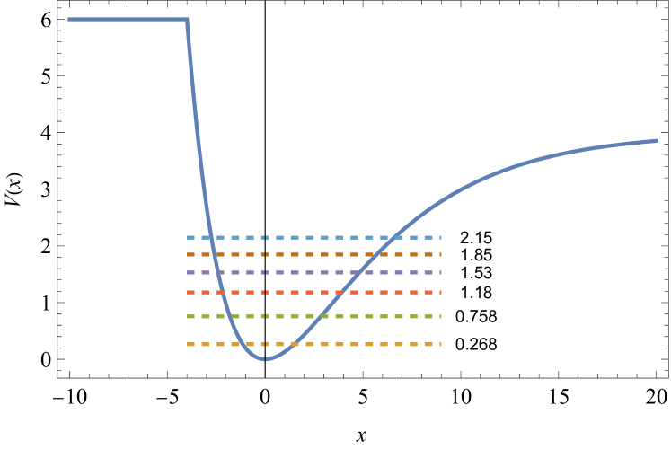
Figure 1: The Morse potential $U\left(x\right)$ used in this example. The dashed lines indicate the low lying energy eigenvalues.

III Validation: Morse oscillator

The example for our method is a Morse oscillator coupled to the environment at inverse temperature $\beta_{e}$. The particle has mass $m=1$ and the truncated Morse potential is $U\left(x\right)=\max\left[U_{max},V_{\infty}\left(1-e^{-ax}\right)^{2}\right]$ (see Fig. 1), with $V_{\infty}=4$, $a=0.2$, and $U_{max}=6$. As before, we use atomic units: $a_{0}$ (Bohr radius) for lengths , $E_{h}$ (Hartree energy) for energy, $m_{e}$ (electron mass) for mass and $\hbar E_{h}^{-1}$ for time. The wave functions $\psi\left(x\right)$ we consider here may have non zero values only in the interval $x\in\left[-10,30\right]$. We represent the system on a 31-point grid of unit spacing ($\Delta x=1$):

$$x_{n}=-10+n\Delta x,\quad n=0,\dots,30.$$ (15)

The wave functions map into the vectors $\psi_{n}=\psi\left(x_{n}\right)$. The position ($\mathcal{X}$) and potential $\mathcal{U}_{0}\equiv U\left(\mathcal{X}\right)$ operators operate as $\left(\mathcal{X}\psi\right)_{n}=x_{n}\psi_{n}$ and $\left(\mathcal{U}_{0}\psi\right)_{n}=U\left(x_{n}\right)\psi_{n}$ respectively. The kinetic energy operator is the finite difference operator $\left(\mathcal{K}_{0}\psi\right)_{n}=-\frac{\hbar^{2}}{2m\Delta x^{2}}\left(\psi_{n-1}-2\psi_{n}+\psi_{n+1}\right)$, combined with the boundary condition $\psi_{-1}\equiv\psi_{31}\equiv 0$. This defines the Hamiltonian $\mathcal{H}_{0}=\mathcal{K}_{0}+\mathcal{U}_{0}$. The lowest lying bound energy levels of this Hamiltonian, determined by diagonalization, are given in Fig. 1.

We take only two Lindblad operators

$$\mathcal{L}_{\pm\omega_{B},\mathcal{T}}=\sqrt{\gamma_{\pm\omega_{B}}}\times\frac{1}{2\mathcal{T}}\int_{-\mathcal{T}}^{\mathcal{T}}e^{\pm i\omega_{B}\tau}\mathcal{X}_{H}\left(\tau\right)d\tau$$ (16)

where $\mathcal{X}_{H}\left(\tau\right)=e^{\frac{i}{\hbar}\mathcal{H}_{0}\tau}\mathcal{X}e^{-\frac{i}{\hbar}\mathcal{H}_{0}\tau}$ is the time-dependent Heisenberg operator for $\mathcal{X}$, $\mathcal{T}=10$ and $\omega_{B}=\hbar^{-1}\left(E_{1}-E_{0}\right)=\hbar^{-1}\times 0.4903$. The rates in Eq. (16) are chosen as

$$\gamma_{\pm\omega_{B}}=\frac{\gamma_{0}}{1+e^{\pm\beta_{e}\hbar\omega_{B}}}$$

where $\gamma_{0}=0.2$ and the environment inverse temperature $\beta_{e}=4$. These rates obey the detailed balance condition

$$\frac{\gamma_{\omega_{B}}}{\gamma_{-\omega_{B}}}=e^{-\beta_{e}\hbar\omega_{B}}.$$ (17)

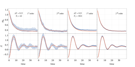
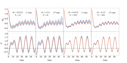
Figure 2: The 95% confidence region (blue shade) for the energy (top panels) and position (bottom panels) transients of the free (left) and driven (right) Morse oscillator starting from a hot state, obtained from the first- and second-order solutions of the ISE (Eqs. (9) and (12)) using $N_{s}=64$ and $1024$ samples. Also shown, as red lines, the numerically exact energy and position transients calculated by solving Eq. (1).

The last element of the model problem is the initial state, which we take as a pure state $\rho\left(0\right)=\left|\xi\right\rangle\left\langle\xi\right|$:

$$\left|\xi\right\rangle =\frac{1}{\sqrt{3}}\left(\left|\psi_{2}\right\rangle+\left|\psi_{3}\right\rangle+\left|\psi_{4}\right\rangle\right)$$ (18)

where $\left|\psi_{n}\right\rangle$ are the eigenvectors of the Hamiltonian operator $\mathcal{H}_{0}$.

III.1 The ’free’ oscillator

We first discuss a time-independent case, where the oscillator is free, i.e., is not subjected to an external driving force beyond the interaction with the environment. Using a small time step and a fourth-order Runge-Kutta propagator, we evolve the density operator according to the Lindblad Equation (Eq. 1), starting from $\rho\left(t=0\right)$ and obtain highly accurate reference values for benchmarking the stochastic propagators. We find that the extended time limit of the evolved state is close, but not exactly equal, to the thermal state at the environment temperature. In order to converge fully into the thermal state, we need to provide more Lindblad operators than just the two we consider here.

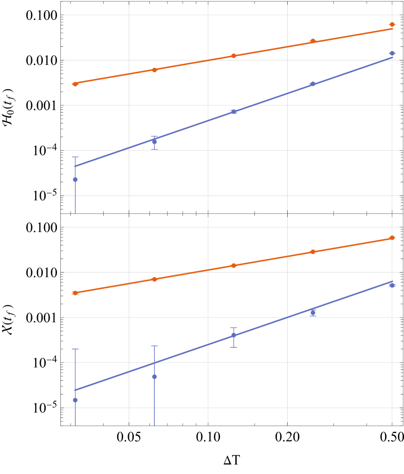
Figure 3: Log-plots showing the first- (red) and second- (blue) order confidence intervals for the energy $\mathcal{H}_{0}\left(t_{f}\right)$ (top panel) and position $\mathcal{X}\left(t_{f}\right)$ (bottom panel) expectation values at $t_{f}=7$ vs the time step $\Delta T$. Dotted straight lines show asymptotic first- and second- order behavior (Eq. (19)). The number of samples used for estimating the confidence intervals was $N_{s}=64\times 10^{6}$.

The stochastic calculation provides confidence intervals for the Lindblad expectation values $\text{Tr}\left[\rho_{t}\mathcal{A}\right]$ of any given observable of interest $\mathcal{A}$. The procedure is a straightforward application of statistical analysis. We run our propagator $N_{s}$ times (with independent random numbers) collecting $N_{s}$ samples of quantum expectation values $A_{t}^{\left(k\right)}\equiv\left\langle\Psi_{t}^{\left(k\right)}\left|\mathcal{A}\right|\Psi_{t}^{\left(k\right)}\right\rangle/\left\langle\Psi_{t}^{\left(k\right)}\left|\Psi_{t}^{\left(k\right)}\right.\right>$ ($k=1,\dots,N_{s}$) and then construct the 95% confidence interval as $\left[\bar{A}_{t}-\Delta A_{t},\bar{A}_{t}+\Delta A_{t}\right]$, where $\bar{A}_{t}$ is the sample average, $\Delta A_{t}=2\times S_{t}/\sqrt{N_{s}}$ is the interval width, and $S_{t}$ is the sample standard deviation. The factor 2 is the large sample t-factor corresponding to a confidence level of $\sim 95\%$. In Fig. 2, we show confidence intervals for two observables, the energy $\mathcal{H}_{0}$ and the position $\mathcal{X}$, using $N_{s}=64$ and $1024$ samples based on the first- and second-order propagators with time step $\Delta T=0.25$. For reference, the figure also shows, as a red solid line, the numerically exact expected value $\mathbb{E}\left[\left\langle\psi_{t}\left|\mathcal{A}\right|\psi_{t}\right\rangle\right]=\text{Tr}\left[\rho_{t}\mathcal{A}\right]$.

The first-order calculation exhibits a noticeable energy bias at $\Delta T=0.25$, even when the confidence interval is broad (when $N_{s}=64$). At the same time, the bias from the second-order calculation is not noticeable even for $N_{s}=1024$ sampling. We discuss the weak order convergence comparing first- and second-order methods below. The standard deviation $S_{t}$ in the first- and second-order calculations is around 0.08 for the energy and 0.6 for the position; interestingly, it does not grow with time. We also checked the algorithm for the case of over-damped dynamics where a parameter of $\gamma=0.6$ was used. We observed similar trends as in weak coupling in terms of the accuracy of the calculation (see details in the supplementary material). In terms of stability, both first- and second- order calculations required time steps of at least 0.0625, for larger time steps the solution was unstable and diverged.

In a weak order-$o$ method $\mathbb{E}\left[\left\langle\Psi_{t}\left|\mathcal{A}\right|\Psi_{t}\right\rangle\right]$ should approach the exact value $\text{Tr}\left[\rho_{t}\mathcal{A}\right]$ as the $o$ power of $\Delta T$. More precisely, there exist $\Delta T_{0}>0$ and $C>0$ such that:

$$\Delta T<\Delta T_{0}\Rightarrow\left|\mathbb{E}\left[\left\langle\Psi_{t}\left|\mathcal{A}\right|\Psi_{t}\right\rangle\right]-\text{Tr}\left[\rho_{t}\mathcal{A}\right]\right|\leq C\times\Delta T^{o}.$$ (19)

To test whether this condition is obeyed we need to know $\mathbb{E}\left[\left\langle\Psi_{t}\left|\mathcal{A}\right|\Psi_{t}\right\rangle\right]$, and this not available directly. However we can build a very small 95% confidence interval by extensive sampling (taking $N_{s}=64\times 10^{6}$), as shown in Fig. 3 for the energy and position observables at time $t_{f}=7$ as function of the time step $\Delta T$. The asymptotic behavior of Eq. (19) is clearly seen as the asymptotic lines do indeed fit through the very small confidence intervals. The power of the second-order calculations is also evident as its error with $\Delta T=0.25$ is smaller than the error in the first-order calculation using a time step smaller by a factor 8.

To assess the utility of the second-order vs the first-order solvers, we note that for the example given here, the wall-time for the former is only a 1.5 times larger than the latter. This small ratio in wall-times will characterize larger systems, as long as there is only one Lindblad operators. From the discussion above, concerning the time-step (and hence number of time steps) required by both methods we conclude that in the present example, the second-order solver is five times more efficient than the first-order one, for low-accuracy calculations. For higher accuracies, it is considerably more efficient. However, the wall time in the second-order calculation depends quadratically on the number $N_{L}$ of Lindblad operators, while that of the first-order is linear in $N_{L}$. Hence, the numerical cost of the second-order calculation may exceed that of the first-order calculation as $N_{L}$ grows.

We mention briefly that linear unraveling (Eq. (14)) has a variance one to two orders of magnitude larger than for the nonlinear unraveling (and it grows linearly with time). Hence, the nonlinear unraveling is expected to be superior in actual applications.

III.2 The driven oscillator

In this example, we subject the Morse oscillator to a driving time-dependent field

$$\mathcal{V}_{0}\theta\left(t\right)=\mathcal{X}\mathcal{F}\sin\left(\omega t\right)$$ (20)

with $\mathcal{F}=0.2$ and $\omega=0.49$. The frequency is resonant between the ground and the first excited states of the oscillator. In Fig. 2 (right) we show first- and second-order results for $N_{s}=64$ and $1024$ samples. The oscillator starts from the same pure state as in the example of the previous section (see Eq. (18)). Under the driving force it strives to cool due to the interaction with the cold environment but the driving field acts to heat it. Eventually, a quasi-stationary non-thermal state forms, with the oscillator energy and position oscillating strongly in time. The first-order solution is unstable for $\Delta T>0.03125$ and even at this small time-step exhibits a large energy bias (red line not passing in the confidence interval for $N_{s}=1024$). The second-order results are stable and much more accurate even when $\Delta T=0.125$. As for the standard deviation $S_{t}$ in the driven oscillator, it is around 0.25 for energy and 0.6 for position. As with the free oscillator, $S_{t}$ does not grow with time.

IV Conclusions

We have presented a weak second-order method for solving the Itô-Schrödinger equation related to quantum state diffusion unraveling of the Lindblad equation. One of the approach’s critical characteristics is working in the interaction picture, helping stability and accuracy even for relatively large time steps. Another significant characteristic of our approach is nonlinear unraveling, using within the equation the expectation value of the Lindblad operator, which reduces the variance (in comparison to the linear unraveling schemes). Moreover, the use of explicitly normalized expectation values of the Lindblad operators (Eq. (4)), further stabilizes the propagation. Another characteristic of our approach is using exact derivatives, which are readily available since our nonlinearity is analytical, for the Itô-Taylor expansion (as opposed to other second-order approaches, such as the Runge-Kutta method, which bypasses derivatives using finite difference). Lastly, our method uses complex Wiener processes.

We have tested the method on the problem of cooling an initially hot Morse oscillator coupled to a colder environment. We studied both a free and a driven oscillator. In both cases, we showed good accuracy of the second-order method when the time step was $\Delta T\omega_{B}\approx 0.1$ or smaller, achieving useful confidence intervals with a relatively small amount of sampling.

We have used 1D examples to benchmark our methods. For such small systems, unraveling does not save computational resources relative to a complete solution of the Lindblad equation. However, the latter method has cubic scaling in wall time and quadratic scaling in memory, and therefore, unraveling can become more efficient as systems grow. One clear advantage of unraveling is that it does not require storing the density matrix, saving a vast amount of computer memory. Furthermore, the most intensive part of the unraveling calculation, namely transforming to and from the interaction picture, can be accomplished by iterative methods [37, 38] involving a fixed number of Hamiltonian applications to any given ket. As systems grow, this latter operation becomes linear-scaling in complexity, endowing the entire unraveling procedure with the same complexity. Thus, there is a massive reduction in computational time relative to a complete solution of the Lindblad equation in the limit of large systems. Furthermore, multiprocessor parallelization can easily overcome the burden of repeated sampling in the unraveling procedure.

The propagator developed in the present paper is our first step towards a more general goal of constructing a framework for studying quantum decoherence and dissipation in large molecular and nanoscale systems. The computational wall-time involved in the second-order calculation scales quadratically with the number $N_{L}$ of Lindblad operators. Therefore, our immediate future work will involve a method to contract Lindblad operators so that a small, hopefully, system-size-independent number of operators can be used. In addition, in the future, we may try to develop solvers for stochastic Schrödinger equations that unravel non-Markovian master equations. Such solvers are required since the Markovian dynamics may result in unreliable predictions of bath-induced coherences [39, 40, 41, 42]).

Supplementary Material

Supplementary material is given on the derivation of Eq. (12) and on the results of the Morse oscilator in the overdamped limit.

Acknowledgments

The authors gratefully acknowledge funding from the Israel Science Foundation grant number ISF-800/19.

References

- [1] W. Thomas Pollard and Richard A. Friesner. Solution of the Redfield equation for the dissipative quantum dynamics of multilevel systems. The Journal of Chemical Physics, 100(7):5054–5065, April 1994.
- [2] D. Kohen, C. C. Marston, and D. J. Tannor. Phase space approach to theories of quantum dissipation. J. Chem. Phys., 107(13):5236–5253, 1997.
- [3] Abraham Nitzan. Chemical dynamics in condensed phases : relaxation, transfer and reactions in condensed molecular systems. Oxford graduate texts. Oxford University Press, Oxford ; New York, 2006.
- [4] Upendra Harbola, Massimiliano Esposito, and Shaul Mukamel. Quantum master equation for electron transport through quantum dots and single molecules. Phys. Rev. B, 74(23):235309, December 2006.
- [5] Heinz-Peter Breuer and Francesco Petruccione. The Theory of Open Quantum Systems. Oxford University Press, January 2007.
- [6] Heiko Appel and Massimiliano Di Ventra. Stochastic quantum molecular dynamics. Phys. Rev. B, 80(21):212303, December 2009.
- [7] Ángel Rivas and Susana F. Huelga. Open quantum systems: an introduction. SpringerBriefs in physics. Springer, Heidelberg, 2012. OCLC: 759533862.
- [8] R Biele and R D’Agosta. A stochastic approach to open quantum systems. J. Phys.: Condens. Matter, 24(27):273201, July 2012.
- [9] Karl Blum. Density Matrix Theory and Applications, volume 64 of Springer Series on Atomic, Optical, and Plasma Physics. Springer Berlin Heidelberg, Berlin, Heidelberg, 2012.
- [10] Gernot Schaller. Open quantum systems far from equilibrium, volume 881. Springer, 2014.
- [11] Crispin Gardiner and Peter Zoller. The Quantum World of Ultra-Cold Atoms and Light Book I: Foundations of Quantum Optics. World Scientific Publishing Company, March 2014.
- [12] Raam Uzdin and Ronnie Kosloff. Speed limits in Liouville space for open quantum systems. EPL, 115(4):40003, August 2016.
- [13] Robert Alicki and Ronnie Kosloff. Introduction to Quantum Thermodynamics: History and Prospects. In F Binder, L. Correa, C Gogolin, J Anders, and G Adesso, editors, Thermodynamics in the Quantum Regime, volume 195 of Fundamental Theories of Physics. Springer, Cham, 1 edition, January 2018. arXiv: 1801.08314.
- [14] Zhu Ruan and Roi Baer. Unravelling open-system quantum dynamics of non-interacting Fermions. Mol. Phys., 116:2490–2496, 2018.
- [15] Gershon Kurizki and Abraham G. Kofman. Thermodynamics and Control of Open Quantum Systems. Cambridge University Press, 1 edition, December 2021.
- [16] Amikam Levy, Eran Rabani, and David T. Limmer. Response theory for nonequilibrium steady states of open quantum systems. Phys. Rev. Res., 3(2):023252, June 2021. Publisher: American Physical Society.
- [17] Matthew Gerry and Dvira Segal. Full counting statistics and coherences: Fluctuation symmetry in heat transport with the unified quantum master equation. Phys. Rev. E, 107(5):054115, May 2023.
- [18] A. G. Redfield. On the Theory of Relaxation Processes. IBM J. Res. & Dev., 1(1):19–31, January 1957.
- [19] P. Gaspard and M. Nagaoka. Slippage of initial conditions for the Redfield master equation. The Journal of Chemical Physics, 111(13):5668–5675, October 1999.
- [20] M. Esposito and M. Galperin. Self-Consistent Quantum Master Equation Approach to Molecular Transport. J. Phys. Chem. C, 114(48):20362–20369, 2010.
- [21] Tobias Becker, Ling-Na Wu, and André Eckardt. Lindbladian approximation beyond ultraweak coupling. Phys. Rev. E, 104(1):014110, July 2021.
- [22] G. Lindblad. On the Generators of Quantum Dynamical Semigroups. Commun. Math. Phys., 48(2):119–130, 1976.
- [23] Vittorio Gorini, Andrzej Kossakowski, and E. C. G. Sudarshan. Completely positive dynamical semigroups of N -level systems. Journal of Mathematical Physics, 17(5):821–825, May 1976.
- [24] Robert Alicki and Karl Lendi. Quantum Dynamical Semigroups and Applications, volume 717 of Lecture Notes in Physics. Springer, Berlin Heidelberg, 2007.
- [25] Daniel Manzano. A short introduction to the Lindblad master equation. AIP Advances, 10(2):025106, February 2020.
- [26] M. B. Plenio and P. L. Knight. The quantum-jump approach to dissipative dynamics in quantum optics. Rev. Mod. Phys., 70(1):101–144, January 1998. Publisher: American Physical Society.
- [27] Ian Percival. Quantum state diffusion. Cambridge University Press, 1998.
- [28] Jean Dalibard, Yvan Castin, and Klaus Mølmer. Wave-function approach to dissipative processes in quantum optics. Phys. Rev. Lett., 68(5):580–583, February 1992.
- [29] C. W. Gardiner, A. S. Parkins, and P. Zoller. Wave-function quantum stochastic differential equations and quantum-jump simulation methods. Phys. Rev. A, 46(7):4363–4381, October 1992.
- [30] Howard Carmichael. An open systems approach to quantum optics: lectures presented at the Université Libre de Bruxelles, October 28 to November 4, 1991, volume 18. Springer Science & Business Media, 1993.
- [31] N. Gisin and I. C. Percival. The Quantum-State Diffusion-Model Applied to Open Systems. Journal of Physics a-Mathematical and General, 25(21):5677–5691, 1992.
- [32] Jingze Li and Xiantao Li. Exponential integrators for stochastic Schrödinger equations. Phys. Rev. E, 101(1):013312, January 2020.
- [33] Carlos M Mora and Mario Muñoz. On the rate of convergence of an exponential scheme for the non-linear stochastic Schrödinger equation with finite-dimensional state space. Phys. Scr., 98(6):065226, June 2023.
- [34] J.R. Johansson, P.D. Nation, and Franco Nori. QuTiP 2: A Python framework for the dynamics of open quantum systems. Computer Physics Communications, 184(4):1234–1240, April 2013.
- [35] Peter E Kloeden and Eckhard Platen. Numerical Solution of Stochastic Differential Equations. Springer, 1992.
- [36] G. N. Milstein. Numerical Integration of Stochastic Differential Equations. Springer Netherlands, Dordrecht, 1995.
- [37] M. D Feit, J. A Fleck, and A Steiger. Solution of the Schrödinger equation by a spectral method. Journal of Computational Physics, 47(3):412–433, September 1982.
- [38] Ronnie Kosloff. Time-dependent quantum-mechanical methods for molecular dynamics. The Journal of Physical Chemistry, 92(8):2087–2100, 1988. Publisher: ACS Publications.
- [39] M. Leijnse and M. R. Wegewijs. Kinetic equations for transport through single-molecule transistors. Phys. Rev. B, 78(23):235424, December 2008. Publisher: American Physical Society.
- [40] Massimiliano Esposito, Maicol A. Ochoa, and Michael Galperin. Efficiency fluctuations in quantum thermoelectric devices. Phys. Rev. B, 91(11):115417, March 2015. Publisher: American Physical Society.
- [41] Yi Gao and Michael Galperin. Simulation of optical response functions in molecular junctions. The Journal of chemical physics, 144(24), 2016. Publisher: AIP Publishing.
- [42] Lyran Kidon, Eli Y. Wilner, and Eran Rabani. Exact calculation of the time convolutionless master equation generator: Application to the nonequilibrium resonant level model. The Journal of Chemical Physics, 143(23):234110, December 2015.