Magic Can Enhance the Quantum Capacity of Channels

Abstract

We investigate the role of magic in the quantum capacity of channels. We consider the quantum channel of the recently proposed discrete beam splitter with the fixed environment state. We find that if the fixed environment state is a stabilizer state, then the quantum capacity is zero. Moreover, we find that the quantum capacity is nonzero for some magic states, and the quantum capacity increases linearly with respect to the number of single-qudit magic states in the environment. These results suggest that magic can increase the quantum capacity of channels, which sheds new insight into the role of stabilizer and magic states in quantum communication.

I Introduction

Stabilizer states and circuits are basic concepts in discrete-variable (DV) quantum systems. They have applications ranging from use in quantum error correction codes, to understanding the possibility of a quantum computational advantage. The importance of stabilizer states was recognized by Gottesman Gottesman (1997) in his study of quantum error correction codes. Quantum error correction codes based on stabilizer states are called stabilizer codes. Shor’s 9-qubit-code Shor (1995) and Kitaev’s toric code Kitaev (2003) are two well-known examples of stabilizer codes.

A stabilizer vector is a common eigenstate of an abelian subgroup of the qubit Pauli group; such a vector defines a pure stabilizer state. Stabilizer circuits comprise Clifford unitaries acting on stabilizer inputs and measurements. These circuits can be efficiently simulated on a classical computer, a result known as the Gottesman-Knill theorem Gottesman (1998). Hence, non-stabilizer resources are necessary to achieve a quantum computational advantage.

The property of not being a stabilizer has recently been called “magic” Bravyi and Kitaev (2005). To quantify the amount of magic, several measures have been proposed Veitch et al. (2012, 2014); Bravyi and Gosset (2016); Bravyi et al. (2016); Howard and Campbell (2017); Bravyi et al. (2019); Bu and Koh (2019); Seddon et al. (2021); Bu et al. (2022a, b); Wang et al. (2019); Bu et al. (2023a); Beverland et al. (2020); Bu and Koh (2022); Leone et al. (2022); Jiang and Wang (2023). These measures have been applied to the classical simulation of quantum ircuits Bravyi and Gosset (2016); Bravyi et al. (2016); Howard and Campbell (2017); Bravyi et al. (2019); Bu and Koh (2019); Seddon et al. (2021), to unitary synthesis Howard and Campbell (2017); Beverland et al. (2020), and to the generalization of capacity in quantum machine learning Bu et al. (2022b, 2023a).

One important measure proposed by Bravyi, Smith, and Smolin is called stabilizer rank Bravyi et al. (2016). They used this measure to investigate time complexity in classical simulation of quantum circuits; here the simulation algorithm is based on a low-rank decomposition of the tensor products of magic states into stabilizer states.

Pauli rank is defined as the number of nonzero coefficients in the decomposition in the Pauli basis. This provides a lower bound on the stabilizer rank Bu and Koh (2019). To achieve a quantum advantage for DV quantum systems, several sampling tasks have been proposed Jozsa and Van den Nest (2014); Koh (2017); Bouland et al. (2018a); Boixo et al. (2018); Bouland et al. (2018b); Bremner et al. (2010); Yoganathan et al. (2019). Some of these proposals have been realized in experiments, which were used to claim a computational advantage over classical supercomputers Arute et al. (2019); Wu et al. (2021); Zhu et al. (2022).

In earlier work, we introduced a discrete beam splitter unitary, enabling us to define a quantum convolution on DV quantum systems. We developed this into a framework to study DV quantum systems, including the discovery of a quantum central limit theorem that converges to a stabilizer state. This means that repeated quantum convolution with a given state converges to a stabilizer state. In other words, stabilizer states can be identified as “quantum-Gaussian” states Bu et al. (2023b, c, d).

One key insight emerging from this point of view is that stabilizer states are the only extremizers of some information theoretic inequalities Bu et al. (2023b, c). Furthermore, we have proposed a convolution-swap test, to determine whether a given state $\rho$ lies in the set of stabilizer states, or whether it is close to being a stabilizer state Bu et al. (2023d).

I.1 Channel Capacity

The quantum capacity of a channel quantifies the maximal number of qubits, on average, that can be reliably transmitted. In this work, we focus on the quantum capacity of the discrete beam splitter with fixed environmental states.

In continuous-variable (CV) quantum systems, the quantum capacity of the beam splitter plays an important role in quantum communication. For example, in optical communication one refers to the CV beam splitter with a thermal environment as a “thermal attenuator channel.” This can be generalized to a general attenuator channel by choosing non-thermal or non-Gaussian environmental states.

There has been a surge of interest in exploring the quantum capacity of such channels Holevo and Werner (2001); Caruso et al. (2006); Wolf et al. (2007); Wilde et al. (2012); Pirandola et al. (2017); Sabapathy and Winter (2017); Wilde and Qi (2018); Rosati et al. (2018); Noh et al. (2019, 2020); Lami et al. (2020a); Oskouei et al. (2022). This interest can be traced to the requirement of applications in quantum information and computation, including universal quantum computation Menicucci et al. (2006); Ohliger et al. (2010), quantum error correction codes Niset et al. (2009), entanglement manipulation Eisert et al. (2002); Fiurášek (2002); Giedke and Ignacio Cirac (2002); Hoelscher-Obermaier and van Loock (2011); Namiki et al. (2014), and non-Gaussian resource theory Lami et al. (2018); Takagi and Zhuang (2018); Lami et al. (2020b). Furthermore, bosonic error-correcting codes, such as the Gottesman-Kitaev-Preskill code Gottesman et al. (2001), has been demonstrated to achieve quantum capacity in these models up to a constant gap Noh et al. (2019).

A nice formula for quantum capacity based on regularized, coherent information has been obtained in the works of Lloyd Lloyd (1997), Shor Shor (2002), and Devetak Devetak (2005). One surprising property of the quantum capacity is super-additivity DiVincenzo et al. (1998); Smith and Yard (2008); Smith et al. (2011); Cubitt et al. (2015). This means that the quantum capacity of the tensor product of channels is larger that the sum of their individual quantum capacities. From this one infers that entanglement can enhance the quantum capacity.

In this work, we investigate the quantum capacity of DV beam splitter, with different choices of environment states. The main results of our work include:

1. If the fixed environment state is a convex linear combination of stabilizer states, then the quantum capacity is zero for the discrete beam splitter with nontrivial parameters. This differs from the CV case, where the presence of Gaussian states leads to a nonzero quantum capacity for some CV beam splitter with nontrivial parameters Lami et al. (2020a).

2. We find that the quantum capacity is nonzero for some magic states, and the quantum capacity increases linearly with respect to the number of single-qudit magic states in the environment. This suggests that magic can increase the quantum capacity of channels.

3. We show that environment states, which are symmetric under the discrete phase space inversion operator, could also lead to zero quantum capacity. We provide some magic state which satisfies this symmetry. This shows that magic is necessary, but not sufficient, to increasing the quantum capacity in this model.

II Basic Framework

We focus on an $n$-qudit system with Hilbert space $\mathcal{H}^{\otimes n}$. Here $\mathcal{H}\simeq\mathbb{C}^{d}$ is $d$-dimensional, and $d$ is a natural number. Let $D(\mathcal{H}^{\otimes n})$ denote the set of all quantum states on $\mathcal{H}^{\otimes n}$. We consider the orthonormal, computational basis in $\mathcal{H}$ denoted by $\set{\ket{k}}$, for ${k\in\mathbb{Z}_{d}}$. The Pauli $X$ and $Z$ operators are

$$X:|k\rangle\mapsto|k+1\rangle\;,\;\;\;Z:|k\rangle\mapsto\omega^{k}_{d}\,|k\rangle,\;\;\;\forall k\in\mathbb{Z}_{d}\;.$$

Here $\mathbb{Z}_{d}$ is the cyclic group over $d$, and $\omega_{d}=\exp(2\pi i/d)$ is a $d$-th root of unity. In order to define our quantum convolution, we assume $d$ is prime.

If $d$ is an odd prime number, the local Weyl operators (or generalized Pauli operators) are defined as

$$w(p,q)=\omega^{-2^{-1}pq}_{d}\,Z^{p}X^{q}\;.$$

Here $2^{-1}$ denotes the inverse $\frac{d+1}{2}$ of 2 in $\mathbb{Z}_{d}$. In the $n$-qudit system, the Weyl operators are defined as $w(\vec{p},\vec{q})=w(p_{1},q_{1})\otimes...\otimes w(p_{n},q_{n}),$ with $\vec{p}=(p_{1},p_{2},...,p_{n})\in\mathbb{Z}^{n}_{d}$, and $\vec{q}=(q_{1},...,q_{n})\in\mathbb{Z}^{n}_{d}$.

Denote $V^{n}:=\mathbb{Z}^{n}_{d}\times\mathbb{Z}^{n}_{d}$; this represents the phase space for $n$-qudit systems, in analogy with continuum mechanics Gross (2006). The functions $w(\vec{p},\vec{q})$ on phase space form an orthonormal basis with respect to the inner product $\langle A,B\rangle=\frac{1}{d^{n}}\operatorname{Tr}\left[A^{\dagger}B\right]$.

The characteristic function $\Xi_{\rho}:V^{n}\to\mathbb{C}$ of a quantum state $\rho$ is

$$\Xi_{\rho}(\vec{p},\vec{q}):=\operatorname{Tr}\left[\rho w(-\vec{p},-\vec{q})\right].$$

Hence, any quantum state $\rho$ can be written as a linear combination of the Weyl operators

$$\rho=\frac{1}{d^{n}}\sum_{(\vec{p},\vec{q})\in V^{n}}\Xi_{\rho}(\vec{p},\vec{q})w(\vec{p},\vec{q})\;.$$

The transformation from the computational basis to the Pauli basis is the quantum Fourier transform that we consider. It has found extensive uses in a myriad of applications, including discrete Hudson theorem Gross (2006), quantum Boolean functions Montanaro and Osborne (2010), quantum circuit complexity Bu et al. (2022a), quantum scrambling Garcia et al. (2023), the generalization capacity of quantum machine learning Bu et al. (2022b), and quantum state tomography Bu et al. (2024).

Denote the vector $|\vec{i}\,\rangle=|i_{1}\rangle\otimes\cdots\otimes|i_{n}\rangle\in\mathcal{H}^{\otimes n}$. In order to define the discrete beam splitter, consider the tensor product Hilbert space of two $n$-qudit Hilbert spaces; we label them system $I$ and $II$ respectively.

Discrete Beam Splitter Bu et al. (2023b, c): Given a prime $d$ and $s,t\in\mathbb{Z}_{d}$ satisfying $s^{2}+t^{2}\equiv 1\mod d$, the discrete beam splitter unitary $U_{s,t}$ for a 2n-qudit system is

$$U_{s,t}=\sum_{\vec{i},\vec{j}\in\mathbb{Z}^{n}_{d}}|s\vec{i}+t\vec{j}\rangle\langle\vec{i}|\otimes|-t\vec{i}+s\vec{j}\rangle\langle\vec{j}|\;.$$ (1)

The quantum channel $\Lambda_{s,\sigma}$ with a fixed environment state $\sigma$ is,

$$\Lambda_{s,\sigma}(\rho):=\operatorname{Tr}_{II}\left[U_{s,t}(\rho\otimes\sigma)U^{\dagger}_{s,t}\right]\;.$$ (2)

The complementary channel is

$$\Lambda^{c}_{s,\sigma}(\rho)=\operatorname{Tr}_{I}\left[U_{s,t}(\rho\otimes\sigma)U^{\dagger}_{s,t}\right].$$ (3)

We denote $\frac{s^{2}\mod d}{d}$ to be the discrete transmission rate, and $\frac{t^{2}\mod d}{d}$ to be the discrete reflection rate. We summarize properties of the discrete beam splitter in Appendix A. In this work, we focus on the discrete beam splitter with nontrivial parameters, i.e., $s^{2},t^{2}\not\equiv 0,1\mod d$.

Remark 1.

In a qubit-system with $d=2$, there is no nontrivial choice of $s,t$ such that $s^{2}+t^{2}\equiv 1\mod 2$, since in that case $(s,t)$ could only be $(0,1)$ or $(1,0)$. Hence, it is impossible to consider the discrete beam splitter with two input states. We give an alternative in Bu et al. (2023d).

III Main results

The quantum capacity of a channel $\Lambda$ can be written as a regularized form of the coherent information, as given by the Lloyd-Shor-Devetak theorem Lloyd (1997); Shor (2002); Devetak (2005):

$$Q(\Lambda) := \lim_{N\to\infty}\frac{Q^{(1)}(\Lambda^{\otimes N})}{N}\;,$$ (4)

$$Q^{(1)}(\Lambda) := \max_{\rho\in D(\mathcal{H}^{\otimes n})}I_{c}(\rho,\Lambda)\;.$$ (5)

Here the coherent information is $I_{c}(\rho,\Lambda):=S(\Lambda(\rho))-S(I\otimes\Lambda(|\Psi\rangle\!\langle\Psi|_{AB}))$, and $\Psi_{AB}$ is a purification of $\rho$.

The coherent information can also be written as $I_{c}(\rho,\Lambda)=S(\Lambda(\rho))-S(\Lambda^{c}(\rho))$, where $\Lambda^{c}$ is the complementary channel of $\Lambda$. In general, it is difficult to calculate the quantum capacity, as it involves the optimization over all states in the asymptotic regime.

Let us now consider the quantum capacity of the quantum channel $\Lambda_{s,\sigma}$ defined in (2) using the discrete beam splitter and the fixed environment state $\sigma$. We start by considering $\sigma$ to be a convex combination of stabilizer states, in order to explore the role of stabilizers.

Theorem 2 (Stabilizer environments yield zero quantum capacity).

Let nontrivial $s,t\in\mathbb{Z}_{d}$ satisfy $s^{2}+t^{2}\equiv 1\mod d$, and let the environment state $\sigma$ be a convex combination of stabilizer states. Then

$$Q(\Lambda_{s,\sigma})=0.$$ (6)

We prove Theorem 2 in Appendix B. This shows that stabilizer environment states ensure that the quantum capacity becomes zero for any nontrivial parameters $s,t$. This phenomenon differs from the CV case in the following way: the CV beam splitter with a pure Gaussian state (e.g., the vacuum state) and with transmissivity $\lambda>1/2$ has a quantum capacity strictly larger than zero Lami et al. (2020a).

From Theorem 2, we infer that a magic environment state is necessary in order to obtain nonzero quantum capacity. Hence, let us consider the case in which the environment state is a magic state. Let $\sigma_{k}$ be a quantum state generated by a Clifford circuit $U_{cl}$ on $k$ copies of 1-qudit magic state $\ket{\text{magic}}$, namely

$$\sigma_{k}=U_{\text{cl}}(|\text{magic}\rangle\!\langle\text{magic}|^{\otimes k}\otimes|0\rangle\!\langle 0|^{n-k})U^{\dagger}_{\text{cl}}\;.$$ (7)

Theorem 3 (Magic can enhance quantum capacity).

Given nontrivial $s,t\in\mathbb{Z}_{d}$ with $s^{2}+t^{2}\equiv 1\mod d$, there exists some 1-qudit magic state $\ket{\text{magic}}$ and a universal constant $c>0$, independent of $d$ and $n$, such that

$$Q(\Lambda_{s,\sigma_{k}})\geq kc\;.$$ (8)

Here, the state $\sigma_{k}$ is given by (7).

We prove Theorem 3 in Appendix C; here we sketch the idea for a very special case. Choose the 1-qudit magic state for the discrete beam splitter to be

$$\ket{\sigma}=\frac{1}{\sqrt{2}}(\ket{0}+\ket{1})\;,$$ (9)

and let the input state be $\rho=\frac{1}{2}(|0\rangle\!\langle 0|+|t^{-1}s\rangle\!\langle t^{-1}s|)$. Then

$$\Lambda_{s,\sigma}(\rho)=\frac{1}{4}(|0\rangle\!\langle 0|+|t\rangle\!\langle t|+|t^{-1}s^{2}\rangle\!\langle t^{-1}s^{2}|+|t^{-1}\rangle\!\langle t^{-1}|),$$

and

$$\Lambda^{c}_{s,\sigma}(\rho)=\frac{1}{2}|0\rangle\!\langle 0|+\frac{1}{4}|-s\rangle\!\langle-s|+\frac{1}{4}|s\rangle\!\langle s|\;,$$

for $s^{2}\not\equiv t^{2}\mod d$. Hence, the coherent information can be written as the entropy difference

$$I_{c}(\rho,\Lambda_{s,\sigma})=S(\Lambda_{s,\sigma}(\rho))-S(\Lambda^{c}_{s,\sigma}(\rho))=\frac{1}{2}\;.$$

Hence, the quantum capacity $Q(\Lambda_{s,\sigma})\geq\frac{1}{2}$, and $Q(\Lambda_{s,\sigma^{\otimes k}\otimes|0\rangle\!\langle 0|^{n-k}})\geq kQ(\Lambda_{s,\sigma})\geq\frac{k}{2}$. If $s^{2}\equiv t^{2}\mod d$, we need some additional arguments.

Let us consider the discrete phase space point operators and their corresponding symmetries. The discrete phase space point operator $A(\vec{p},\vec{q})$ with $(\vec{p},\vec{q})\in V^{n}$ is defined as $A(\vec{p},\vec{q})=w(\vec{p},\vec{q})Aw(\vec{p},\vec{q})^{\dagger}$, where $A$ is given by $A=\frac{1}{d^{n}}\sum_{(\vec{u},\vec{v})\in V^{n}}w(\vec{u},\vec{v})$. These operators can be used to define the discrete Wigner function, where the nongativity of the discrete Wigner function is used to characterize the stabilizer states on qudit systems Gross (2006). The operator $A$ can be rewritten as $A=\sum_{\vec{x}}\ket{-\vec{x}}\bra{\vec{x}}$. In Appendix A, we list some properties of these discrete phase-space point operators for completeness.

Now let us consider symmetry under the discrete phase space point operators. A quantum state $\sigma$ is defined to be symmetric under the discrete phase space inverse operation if

$$A\sigma A^{\dagger}=\sigma.$$ (10)

For example, the zero-mean stabilizer states exhibit this symmetry as the characteristic function of the zero-mean stabilizer states is either 0 or 1.

We now demonstrate that choosing symmetric states as environment states will lead to zero quantum capacity, even though these states could be magic states.

Theorem 4 (Symmetry can limit quantum capacity).

Let $\sigma$ be an $n$-qudit state, which is a convex combination of states $w(\vec{a})\sigma_{\vec{a}}\,w(\vec{a})^{\dagger}$, with each state $\sigma_{\vec{a}}$ having discrete, phase-space, inverse symmetry. Then $\Lambda_{s,\sigma}$ is anti-degradable for $s\equiv t\mod d$, and the quantum capacity

$$Q(\Lambda_{s,\sigma})=0\;.$$ (11)

The proof of Theorem 4 is presented in Appendix D. Combined with the Theorem 2, 3, and 4, we conclude that magic is necessary but not sufficient to increase the quantum capacity of the quantum channel defined by the discrete beam splitter.

Note that, several results show the extremality of stabilizer states in channel capacity, such as the classical capacity. The Holevo capacity is an important quantity that provides a least upper bound on the classical capacity; this is known as the Holevo-Schumacher-Westmoreland theorem Holevo (1998); Schumacher and Westmoreland (1997). It is known that the quantum channel $\Lambda_{\sigma}$ in (2) achieves its maximal Holevo capacity $\sigma$, if and only if $\sigma$ is a pure stabilizer state. (See Theorem 19 in Bu et al. (2023b) and Theorem 73 in Bu et al. (2023c) for the details.) These results show that the stabilizer states are the only extremizers of the Holevo capacity given by the discrete beam splitter.

However, this is not the case for quantum capacity as shown in Theorem 4. That is, stabilizer states are not the only extremizers of the quantum capacity in the discrete beam splitter. Here, we give an example of a magic state with zero quantum capacity:

Example 5.

Consider the 1-qudit state

$$\ket{\sigma}=\frac{1}{\sqrt{2}}(\ket{1}+\ket{-1})\;.$$ (12)

The characteristic function of $|\sigma\rangle\!\langle\sigma|$ shows that it is a magic state. This state is also symmetric under the phase inverse operation in (10). Hence from Theorem 4 we infer that the quantum capacity of $\Lambda_{\sigma}$ is zero for $s\equiv t\mod d$.

IV Conclusion

In this work, we provide new understanding of stabilizer and magic states in quantum communication. We show that magic can increase the quantum channel capacity in the model defined by the discrete beam splitter.

It is natural for future work to consider different quantum channel capacities of the discrete beam splitter, such as private capacity Li et al. (2009); Gao et al. (2018). Besides, in qubit systems, it is impossible to consider the discrete beam splitter for two input states and with nontrivial parameters $s,t$; so it would be interesting to consider the channel capacities of $n$-qubit channels to show the power of magic states.

Finally, as the single-qudit magic state (9) is the non-stabilizer encoding of the 1-qubit stabilizer state $\ket{+}$, it is natural to ask if there exists some non-stabilizer error correcting code in a qudit-system, which could achieve the quantum capacity of the DV beam splitter. The study of the Gottesman-Kitaev-Preskill code in the CV beam splitter Noh et al. (2019) may be helpful for understanding this question, as the Gottesman-Kitaev-Preskill code provides non-Gaussian encoding of the stabilizer codes.

V Acknowledgements

We thank Liyuan Chen, Roy Garcia, Marius Junge, Zixia Wei, and Chen Zhao for discussions. This work was supported in part by the ARO Grant W911NF-19-1-0302 and the ARO MURI Grant W911NF-20-1-0082.

Appendix A Properies of the discrete Beam splitter

Unless noted otherwise, here we summarize some results in Bu et al. (2023b, c). For simplicity denote $\Xi_{\rho}(\vec{x})$ with $\vec{x}=(\vec{p},\vec{q})\in V^{n}$.

Proposition 6 (Proposition 35 in Bu et al. (2023c)).

For any $\vec{a},\vec{b}\in V^{n}$, the discrete beam splitter $U_{s,t}$ satisfies

$$U_{s,t}(w(\vec{a})\otimes w(\vec{b}))U^{\dagger}_{s,t}=w(s\vec{a}+t\vec{b})\otimes w(-t\vec{a}+s\vec{b})\;.$$ (13)

Definition 7 (Quantum convolution defined by discrete beam splitter).

The quantum convolution of two $n$-qudit states $\rho$ and $\sigma$ is

$$\rho\boxtimes_{s,t}\sigma=\Lambda_{\sigma}(\rho)=\operatorname{Tr}_{II}\left[U_{s,t}(\rho\otimes\sigma)U^{\dagger}_{s,t}\right].$$ (14)

Definition 8 (Mean state).

Given an $n$-qudit state $\rho$, the mean state $\mathcal{M}(\rho)$ is the operator with the characteristic function:

$$\Xi_{\mathcal{M}(\rho)}(\vec{x}):=\left\{\begin{aligned} &\Xi_{\rho}(\vec{x}),&&|\Xi_{\rho}(\vec{x})|=1,\\ &0,&&|\Xi_{\rho}(\vec{x})|<1.\end{aligned}\right.$$ (15)

The mean state $\mathcal{M}(\rho)$ is a stabilizer state.

Lemma 9 (Gross (2006)).

The set of phase space point operators $\set{A(\vec{p},\vec{q})}_{(\vec{p},\vec{q})\in V^{n}}$ satisfies three properties when the local dimension $d$ is an odd prime:

1. $\set{A(\vec{p},\vec{q})}_{(\vec{p},\vec{q})\in V^{n}}$ forms a Hermitian, orthonormal basis with respect to the inner product defined by $\langle A,B\rangle=\frac{1}{d^{n}}\operatorname{Tr}\left[A^{\dagger}B\right]$.

2. $A(\vec{0},\vec{0})=\sum_{\vec{x}}\ket{-\vec{x}}\bra{\vec{x}}$ in the Pauli $Z$ basis.

3. $A(\vec{p},\vec{q})=w(\vec{p},\vec{q})A(\vec{0},\vec{0})w(\vec{p},\vec{q})^{\dagger}$.

In the main context, we denote $A(\vec{0},\vec{0})$ as $A$ for simplicity.

Lemma 10.

The zero-mean stabilizer state is symmetric under the phase space inverse operator.

Proof.

By simple calculation, we have

$$AZA^{{\dagger}}=\sum_{j}\omega^{j}_{d}A|j\rangle\!\langle j|A^{\dagger}=\sum_{j}\omega^{j}_{d}|-j\rangle\!\langle-j|=Z^{-1},$$ (16)

$$AXA^{{\dagger}}=\sum_{j}A\ket{j+1}\bra{j}A=\sum_{j}\ket{-j-1}\bra{-j}=X^{-1},$$ (17)

which implies that

$$Aw(\vec{p},\vec{q})A^{\dagger}=w(-\vec{p},-\vec{q}).$$ (18)

Hence, we have

$$\Xi_{A\rho A^{\dagger}}(\vec{x})=\Xi_{\rho}(-\vec{x}),\quad\forall\vec{x}\in V^{n}.$$ (19)

Hence, the state $\rho$ is symmetric under the phase space inverse operator iff $\Xi_{\rho}(\vec{x})=\Xi_{\rho}(-\vec{x})$, for any $\vec{x}\in V^{n}$. For a zero-mean stabilizer state $\rho$, we have $\Xi_{\rho}(\vec{x})=\Xi_{\rho}(-\vec{x})$, which is either 0 or 1. Therefore, it is symmetric under the phase space inverse operator.

∎

The phase space point operators can be used to define the discrete Wigner function

$$W_{\rho}(\vec{p},\vec{q})=\operatorname{Tr}\left[\rho A(\vec{p},\vec{q})\right].$$ (20)

One important result about the discrete Wigner function is the discrete Hudson theorem Gross (2006). It states that for any $n$-qudit pure state $\psi$ with odd prime $d$, it is a stabilizer state iff the discrete Wigner function $W_{\psi}$ is nonnegative.

Lemma 11.

The quantum convolution $\boxtimes_{s,t}$ satisfies the following properties:

1. Convolution-multiplication duality: $\Xi_{\rho\boxtimes_{s,t}\sigma}(\vec{x})=\Xi_{\rho}(s\vec{x})\Xi_{\sigma}(t\vec{x})$, for any $\vec{x}\in V^{n}$. (See Proposition 11 in Bu et al. (2023b).)

2. Convolutional stability: If both $\rho$ and $\sigma$ are stabilizer states, then $\rho\boxtimes_{s,t}\sigma$ is still a stabilizer state. (See Proposition 12 in Bu et al. (2023b).)

3. Quantum central limit theorem: Let $\boxtimes^{N}\rho:=(\boxtimes^{N-1}\rho)\boxtimes\rho$ be the $N^{\rm th}$ repeated quantum convolution, and $\boxtimes^{2}\rho=\rho\boxtimes\rho$. Then $\boxtimes^{N}\rho$ converges to a stabilizer state $\mathcal{M}(\rho)$ as $N\to\infty$. (See Theorem 24 in Bu et al. (2023b).)

4. Quantum maximal entropy principle: $S(\rho)\leq S(\mathcal{M}(\rho))$. (See Theorem 4 in Bu et al. (2023b).)

5. Commutativity with Clifford unitaries: For any Clifford unitary $U$, there exists some Clifford unitary $V$ such that $(U\rho U^{\dagger})\boxtimes(U\sigma U^{\dagger})=V(\rho\boxtimes\sigma)V^{\dagger}$ for any input states $\rho$ and $\sigma$. (See Lemma 85 in Bu et al. (2023c).)

6. Wigner function positivity: If $s\equiv t\mod d$, then the discrete Wigner function $W_{\rho\boxtimes\sigma}\geq 0$ for any n-qudit states $\rho$ and $\sigma$. (See Remark 83 in Bu et al. (2023c).)

Appendix B Discrete beam splitter with stabilizer environment state

Lemma 12.

Given a quantum channel $\Lambda=\sum_{i}p_{i}\Lambda_{i}$, we have the following convexity of coherent information,

$$S(\Lambda(\rho))-S(I\otimes\Lambda(|\Psi_{AB}\rangle\!\langle\Psi_{AB}|))\leq\sum_{i}p_{i}[S(\Lambda_{i}(\rho))-S(I\otimes\Lambda_{i}(|\Psi_{AB}\rangle\!\langle\Psi_{AB}|)].$$ (21)

Proof.

By the joint convexity of relative entropy, we have

$$D(I\otimes\Lambda(|\Psi_{AB}\rangle\!\langle\Psi_{AB}|||\frac{I_{A}}{d}\otimes\Lambda(\rho)))\leq\sum_{i}p_{i}D(I\otimes\Lambda_{i}(|\Psi_{AB}\rangle\!\langle\Psi_{AB}|||\frac{I_{A}}{d}\otimes\Lambda_{i}(\rho))),$$ (22)

which is equivalent to

$$S(\Lambda(\rho))-S(I\otimes\Lambda(|\Psi_{AB}\rangle\!\langle\Psi_{AB}|))\leq\sum_{i}p_{i}[S(\Lambda_{i}(\rho))-S(I\otimes\Lambda_{i}(|\Psi_{AB}\rangle\!\langle\Psi_{AB}|)].$$ (23)

∎

Theorem 13 (Restatement of Theorem 2).

Given nontrivial $s,t\in\mathbb{Z}_{d}$ with $s^{2}+t^{2}\equiv 1\mod d$, and the fixed environment state $\sigma$ being any convex combination of stabilizer states, we have

$$Q(\Lambda_{s,\sigma})=0.$$ (24)

Proof.

Let us first prove that $Q^{(1)}(\Lambda_{s,\sigma})=0$, which means that for any $n$-qudit state $\rho$ with the purification $\Psi_{AB}$,

$$S(\Lambda(\rho))-S(I\otimes\Lambda(|\Psi_{AB}\rangle\!\langle\Psi_{AB}|))\leq 0.$$ (25)

By Lemma 12, we only need to consider the case where $\sigma$ is a pure stabilizer state on an $n$-qudit system. Then, there exists some abelian group of Weyl operations with $n$ generators $G_{\sigma}:=\set{w(\vec{x}):w(\vec{x})\sigma=\sigma}$. By a simple calculation, $\Delta(\rho):=\frac{1}{d^{n}}\sum_{w(\vec{x})\in G_{\sigma}}w(\vec{x})\rho w(\vec{x})^{\dagger}$ is the full-dephasing channel, and there exists an orthonormal basis $\ket{\varphi_{\vec{a}}}$ such that

$$w(\vec{x})\ket{\varphi_{\vec{a}}}=\omega^{\vec{x}\cdot\vec{a}}_{d}\ket{\varphi_{\vec{a}}},$$

for any $w(\vec{x})\in G_{\sigma}$, and

$$\Delta(\rho)=\frac{1}{d^{n}}\sum_{\vec{a}\in\mathbb{Z}^{n}_{d}}\bra{\varphi_{\vec{a}}}\rho\ket{\varphi_{\vec{a}}}|\varphi_{\vec{a}}\rangle\!\langle\varphi_{\vec{a}}|.$$

Note that, $\sigma=|\varphi_{\vec{0}}\rangle\!\langle\varphi_{\vec{0}}|$. Let us denote $p_{\vec{a}}=\bra{\varphi_{\vec{a}}}\rho\ket{\varphi_{\vec{a}}}$. Then, we have

$$\Lambda_{\sigma}(\rho)=\Lambda(\rho\otimes\sigma)=\frac{1}{d^{n}}\sum_{w(\vec{x})\in G_{\sigma}}\Lambda(\rho\otimes w(\vec{x})\sigma w(\vec{x})^{\dagger})=\Lambda\left(\frac{1}{d^{n}}\sum_{w(\vec{x})\in G_{\sigma}}w(\vec{x})\rho w(\vec{x})^{\dagger}\otimes\sigma\right)=\Lambda_{\sigma}(\Delta(\rho)),$$ (26)

where the second equality comes from the definition of $G_{\sigma}$, and the third equality comes from the following property (proved as Proposition 41 inBu et al. (2023c)), namely

$$\Lambda(w(\vec{x})\otimes w(\vec{y})\rho_{AB}w(\vec{x})^{\dagger}\otimes w(\vec{y})^{\dagger})=w(s\vec{x}+t\vec{y})\rho_{AB}w(s\vec{x}+t\vec{y})^{\dagger},$$

where $\Lambda(\rho_{I,II})=\operatorname{Tr}_{II}\left[U_{s,t}\rho_{I,II}U^{\dagger}_{s,t}\right]$. Moreover, based on the convolution-multiplication duality in Lemma 11, we have

$$\Xi_{\sigma\boxtimes_{s,t}|\varphi_{\vec{a}}\rangle\!\langle\varphi_{\vec{a}}|}(\vec{x})=\Xi_{|\varphi_{\vec{0}}\rangle\!\langle\varphi_{\vec{0}}|\boxtimes_{s,t}|\varphi_{\vec{a}}\rangle\!\langle\varphi_{\vec{a}}|}(\vec{x})=\Xi_{|\varphi_{\vec{0}}\rangle\!\langle\varphi_{\vec{0}}|}(s\vec{x})\Xi_{|\varphi_{\vec{a}}\rangle\!\langle\varphi_{\vec{a}}|}(t\vec{x})=\omega^{-t\vec{a}\cdot\vec{x}}_{d}\delta_{\vec{x}\in G_{\sigma}}=\Xi_{|\varphi_{t\vec{a}}\rangle\!\langle\varphi_{t\vec{a}}|}(\vec{x}).$$

Hence,

$$\Lambda_{\sigma}(|\varphi_{\vec{a}}\rangle\!\langle\varphi_{\vec{a}}|)=\sigma\boxtimes_{s,t}|\varphi_{\vec{a}}\rangle\!\langle\varphi_{\vec{a}}|=|\varphi_{t\vec{a}}\rangle\!\langle\varphi_{t\vec{a}}|.$$ (27)

Thus,

$$\Lambda_{\sigma}(\rho)=\Lambda_{\sigma}(\Delta(\rho))=\sum_{\vec{a}}p_{\vec{a}}\Lambda_{\sigma}(|\varphi_{\vec{a}}\rangle\!\langle\varphi_{\vec{a}}|)=\sum_{\vec{a}}p_{\vec{a}}|\varphi_{t\vec{a}}\rangle\!\langle\varphi_{t\vec{a}}|.$$ (28)

Similarly, for the purification $\Psi_{AB}$, we have

$$I\otimes\Lambda_{\sigma}(|\Psi_{AB}\rangle\!\langle\Psi_{AB}|)=\sum_{\vec{a}}p_{\vec{a}}\tau^{A}_{\vec{a}}\otimes|\varphi_{t\vec{a}}\rangle\!\langle\varphi_{t\vec{a}}|,$$ (29)

where $\tau^{A}_{\vec{a}}=\operatorname{Tr}\left[|\Psi_{AB}\rangle\!\langle\Psi_{AB}|I\otimes|\varphi_{\vec{a}}\rangle\!\langle\varphi_{\vec{a}}|\right]/p_{\vec{a}}$. Hence, we have

$$S(\Lambda_{\sigma}(\rho)) = S(\vec{p}),$$ (30)

$$S(I\otimes\Lambda_{\sigma}(|\Psi_{AB}\rangle\!\langle\Psi_{AB}|)) = S\left(\sum_{\vec{a}}p_{\vec{a}}\tau^{A}_{\vec{a}}\otimes|\varphi_{t\vec{a}}\rangle\!\langle\varphi_{t\vec{a}}|\right)=S(\vec{p})+\sum_{\vec{a}}p_{\vec{a}}S(\tau^{A}_{\vec{a}})\;.$$ (31)

Here $\vec{p}=\set{p_{\vec{a}}}_{\vec{a}\in\mathbb{Z}^{n}_{d}}$ is the probability distribution. Therefore, we have

$$I_{c}(\rho,\Lambda_{\sigma})\leq 0,$$ (32)

for any input state $\rho$. That is, $Q^{(1)}(\Lambda_{\sigma})=0$. Since $\Lambda^{\otimes N}_{s,\sigma}=\Lambda_{s,\sigma^{\otimes N}}$, and the tensor product of stabilizer states is still a stabilizer state, we can repeat the above proof for $Q^{(1)}(\Lambda^{\otimes N}_{\sigma})$ for any integer $N$. Hence, we have $Q(\Lambda_{\sigma})=0$.

∎

Appendix C Discrete beam splitter with environment state being a magic state

Theorem 14 (Restatement of Theorem 3).

Given nontrivial $s,t\in\mathbb{Z}_{d}$ with $s^{2}+t^{2}\equiv 1\mod d$, there exists some 1-qudit magic state $\ket{magic}$ such that

$$Q(\Lambda_{s,\sigma_{k}})\geq kc,c>0$$ (33)

where $c$ is a universal constant independent of $d$ and $n$, $\sigma_{k}$ is a quantum state generated by any Clifford circuit on $\ket{\text{magic}}^{\otimes k}\otimes\ket{0}^{n-k}$, i.e., $\sigma_{k}=U_{\text{cl}}|\text{magic}\rangle\!\langle\text{magic}|^{\otimes k}\otimes|0\rangle\!\langle 0|^{n-k}U^{\dagger}_{\text{cl}}$.

Proof.

Since the Clifford unitary commutes with the discrete beam splitter, see Lemma 11.5, then

$$Q(\Lambda_{s,\sigma_{k}})=Q(\Lambda_{s,|\text{magic}\rangle\!\langle\text{magic}|^{\otimes k}\otimes|0\rangle\!\langle 0|^{n-k}})=Q(\otimes^{k}\Lambda_{s,\ket{\text{magic}}}\otimes^{n-k}\Lambda_{s,\ket{0}})\geq kQ(\Lambda_{s,\ket{\text{magic}}})\;.$$ (34)

Hence, we only need to consider the single-qudit case. Let us first consider the beam splitter $U_{s,t}$ with $s^{2}\neq t^{2}\mod d$, and single-qudit environment state $\sigma$ to be

$$\ket{\sigma}_{E}=\frac{1}{\sqrt{2}}(\ket{0}_{E}+\ket{1}_{E})\;,$$ (35)

and

$$\ket{\psi}_{AB}=\frac{1}{\sqrt{2}}\left(\ket{0}_{A}\ket{0}_{B}+\ket{t^{-1}s}_{A}\ket{t^{-1}s}_{B}\right)\;.$$ (36)

Then we have

$$\ket{\tau}_{ABE}=U^{BE}_{s,t}\ket{\psi}_{AB}\otimes\ket{\sigma}_{E}=\frac{1}{2}(\ket{0,0,0}_{ABE}+\ket{0,t,s}_{ABE}+\ket{t^{-1}s,t^{-1}s^{2},-s}_{ABE}+\ket{t^{-1}s,t^{-1},0}_{ABE})\;.$$ (37)

And thus

$$\tau_{E}=\frac{1}{2}|0\rangle\!\langle 0|_{E}+\frac{1}{4}|-s\rangle\!\langle-s|_{E}+\frac{1}{4}|s\rangle\!\langle s|_{E},$$ (38)

and

$$\tau_{B}=\frac{1}{4}\left(|0\rangle\!\langle 0|_{B}+|t\rangle\!\langle t|_{B}+|t^{-1}s^{2}\rangle\!\langle t^{-1}s^{2}|_{B}+|t^{-1}\rangle\!\langle t^{-1}|_{B}\right)\;.$$ (39)

Hence

$$I_{c}(\rho,\Lambda_{s,\sigma})=S(\tau_{B})-S(\tau_{AB})=S(\tau_{B})-S(\tau_{E})=\frac{1}{2}\;.$$ (40)

Now, let us consider the case where $s^{2}\equiv t^{2}\mod d$. This can be split into two cases: (a) $s\equiv t\mod$ and (b) $s\equiv-t\mod d$.

Case (a). If $s\equiv t\mod d$, let us consider the environment state

$$\ket{\sigma}_{E}=\sqrt{\frac{2}{5}}\ket{0}_{E}+\sqrt{\frac{3}{5}}\ket{1}_{E}\;,$$ (41)

and

$$\ket{\psi}_{AB}=\frac{\sqrt{6}}{5}\ket{0,0}_{AB}+\frac{3}{5}\ket{0,1}_{AB}+\sqrt{\frac{2}{5}}\ket{1,0}_{AB}\;.$$ (42)

Then we have

$$\ket{\tau}_{ABE} = U^{BE}_{s,s}\ket{\psi}_{AB}\otimes\ket{\sigma}_{E}$$ (43)

$$= \left(\frac{\sqrt{6}}{5}\ket{0}_{A}+\sqrt{\frac{2}{5}}\ket{1}_{A}\right)\otimes\left(\sqrt{\frac{2}{5}}\ket{0,0}_{BE}+\sqrt{\frac{3}{5}}\ket{s,s}_{BE}\right)+\frac{3}{5}\ket{0}_{A}\otimes\left(\sqrt{\frac{2}{5}}\ket{s,-s}+\sqrt{\frac{3}{5}}\ket{2s,0}_{BE}\right)\;.$$ (44)

Thus

$$\tau_{E}=\frac{59}{125}|0\rangle\!\langle 0|_{E}+\frac{6}{25}|s\rangle\!\langle s|_{E}+\frac{36}{125}|\phi\rangle\!\langle\phi|_{E}\;,$$ (45)

where $\ket{\phi}=\frac{1}{\sqrt{2}}(\ket{s}+\ket{-s})$, with spectrum $\lambda_{1}=\frac{59}{125},\ \lambda_{2}=\frac{3(11-\sqrt{61})}{125},\ \lambda_{3}=\frac{3(11+\sqrt{61})}{125}$, and

$$\tau_{B}=\frac{4}{25}|0\rangle\!\langle 0|_{B}+\frac{66}{125}|s\rangle\!\langle s|_{B}+\frac{39}{125}|\varphi\rangle\!\langle\varphi|_{B}\;,$$ (46)

where $\ket{\varphi}=\frac{2}{\sqrt{13}}\ket{0}+\frac{3}{\sqrt{13}}\ket{2s}$, with spectrum $\mu_{1}=\frac{66}{125},\ \mu_{2}=\frac{59+\sqrt{1321}}{250},\mu_{3}=\frac{59-\sqrt{1321}}{250}$. Hence,

$$I_{c}(\rho,\Lambda_{s,\sigma})=S(\tau_{B})-S(\tau_{AB})=S(\tau_{B})-S(\tau_{E})\approx 0.0178.$$ (47)

Case (b). If $s\equiv-t\mod d$, consider the environment state

$$\ket{\sigma}_{E}=\sqrt{\frac{2}{5}}\ket{0}_{E}+\sqrt{\frac{3}{5}}\ket{-1}_{E}\;,$$ (48)

and

$$\ket{\psi}_{AB}=\frac{\sqrt{6}}{5}\ket{0,0}_{AB}+\frac{3}{5}\ket{0,1}_{AB}+\sqrt{\frac{2}{5}}\ket{1,0}_{AB}\;.$$ (49)

Then we have

$$\ket{\tau}_{ABE} = U^{BE}_{s,-s}\ket{\psi}_{AB}\otimes\ket{\sigma}_{E}$$ (50)

$$= \left(\frac{\sqrt{6}}{5}\ket{0}_{A}+\sqrt{\frac{2}{5}}\ket{1}_{A}\right)\otimes\left(\sqrt{\frac{2}{5}}\ket{0,0}_{BE}+\sqrt{\frac{3}{5}}\ket{s,-s}_{BE}\right)+\frac{3}{5}\ket{0}_{A}\otimes\left(\sqrt{\frac{2}{5}}\ket{s,s}_{BE}+\sqrt{\frac{3}{5}}\ket{2s,0}_{BE}\right)\;.$$ (51)

Then the proof is the same as the Case (a). ∎

Appendix D Discrete beam splitter with $s^{2}\equiv t^{2}\mod d$

Let us define the quantum operation $\mathcal{A}$ as

$$\mathcal{A}(\sigma)=A\sigma A^{\dagger}\;.$$ (52)

Then discrere phase space inverse symmetry can be rewritten as

$$\mathcal{A}(\sigma)=\sigma\;.$$ (53)

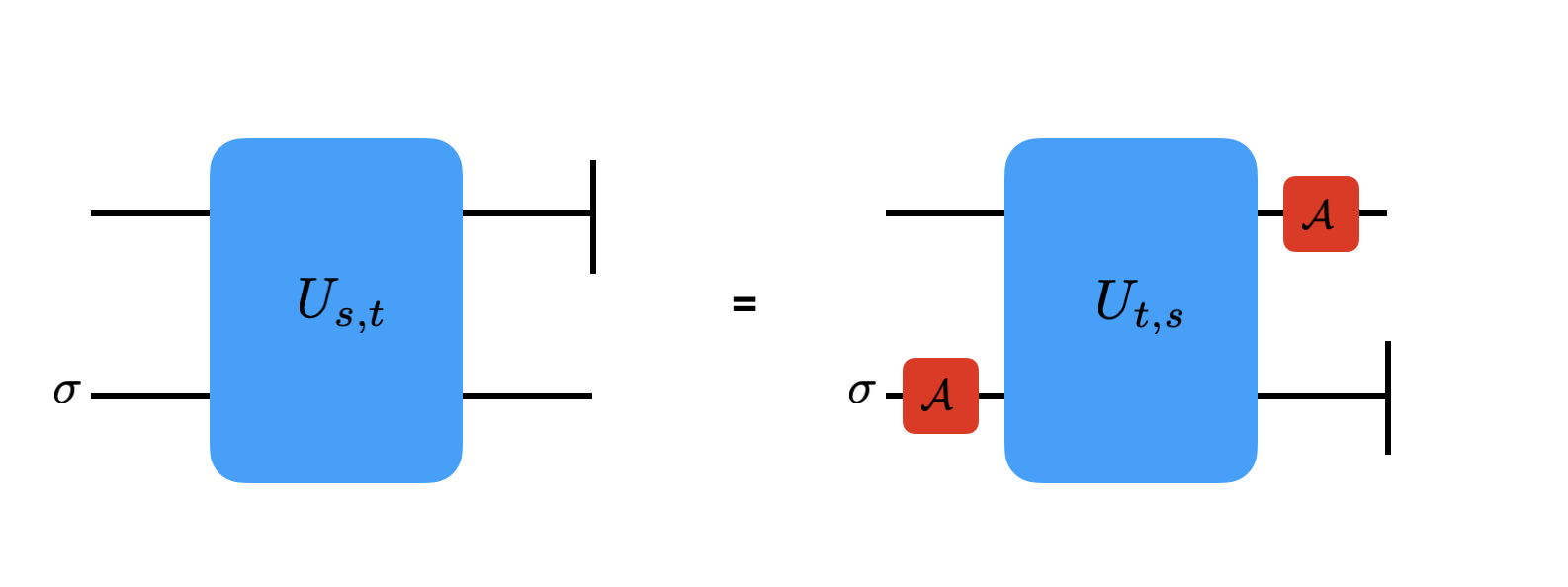
Figure 1: The diagram to show the equivalence of $\Lambda^{c}_{s,\sigma}$ and $\mathcal{A}\circ\Lambda_{t,\mathcal{A}(\sigma)}$.

Lemma 15.

Given $s^{2}+t^{2}\equiv 1\mod d$, we have the relation

$$\Lambda^{c}_{s,\sigma}=\mathcal{A}\circ\Lambda_{t,\mathcal{A}(\sigma)}\;,$$ (54)

for any state $\sigma$ (See Fig. 1).

Proof.

Since the characteristic function $\Xi$ provides a complete description of the states and channels, we only need to consider the characteristic function $\Xi_{\Lambda^{c}_{s,\sigma}(\rho)}$ and $\Xi_{\mathcal{A}\circ\Lambda_{t,\mathcal{A}(\sigma)}(\rho)}$ for any input state $\rho$. Based on the convolution-multiplication duality in Bu et al. (2023b) stated here as Lemma 11, we have

$$\Xi_{\Lambda^{c}_{s,\sigma}(\rho)}(\vec{x})=\Xi_{\rho}(-t\vec{x})\Xi_{\sigma}(s\vec{x})\;,$$ (55)

and

$$\Xi_{\mathcal{A}\circ\Lambda_{t,\mathcal{A}(\sigma)}}(\vec{x})=\Xi_{\rho}(-t\vec{x})\Xi_{\mathcal{A}(\sigma)}(-s\vec{x})=\Xi_{\rho}(-t\vec{x})\Xi_{\sigma}(s\vec{x})\;.$$ (56)

Thus, we have $\Lambda^{c}_{s,\sigma}(\rho)=\mathcal{A}\circ\Lambda_{t,\mathcal{A}(\sigma)}(\rho)$ for any input state $\rho$, i.e., $\Lambda^{c}_{s,\sigma}=\mathcal{A}\circ\Lambda_{t,\mathcal{A}(\sigma)}$. ∎

Theorem 16 (Restatement of Theorem 4).

Let $\sigma$ be an $n$-qudit state, which is some convex combination of $w(\vec{a})\sigma_{\vec{a}}w(\vec{a})^{\dagger}$, with each state $\sigma_{\vec{a}}$ having discrete phase space inverse symmetry. Then $\Lambda_{s,\sigma}$ is anti-degradable for $s\equiv t\mod d$, and

$$Q(\Lambda_{s,\sigma})=0\;.$$ (57)

Proof.

We only need to consider the case where $\sigma=w(\vec{a})\sigma_{0}w(\vec{a})$ where $\sigma_{0}=\mathcal{A}(\sigma_{0})$. By Lemma 15, we have

$$\Lambda^{c}_{s,\sigma}=\mathcal{A}\circ\Lambda_{t,\mathcal{A}(\sigma)}\;.$$ (58)

Moreover,

$$\mathcal{A}(\sigma)=\mathcal{A}(w(\vec{a}))\sigma_{0}\mathcal{A}(w(\vec{a})^{\dagger})=w(-2\vec{a})\sigma w(2\vec{a})\;.$$ (59)

Let us denote $D_{\vec{a}}(\sigma)=w(\vec{a})\sigma w(\vec{a})^{\dagger}$. Hence $\mathcal{A}(D_{\vec{a}}(\sigma))=D_{-2\vec{a}}(\sigma)$. Besides, we have

$$\rho\boxtimes_{t,s}D_{\vec{a}}(\sigma)=D_{s\vec{a}}(\rho\boxtimes_{t,s}\sigma)\;,$$ (60)

based on the following property(See Proposition 41 in Bu et al. (2023c))

$$\Lambda(w(\vec{x})\otimes w(\vec{y})\rho_{AB}w(\vec{x})^{\dagger}\otimes w(\vec{y})^{\dagger})=w(s\vec{x}+t\vec{y})\rho_{AB}w(s\vec{x}+t\vec{y})^{\dagger}\;,$$

where $\Lambda(\rho_{I,II})=\operatorname{Tr}_{II}\left[U_{s,t}\rho_{I,II}U^{\dagger}_{s,t}\right]$. Since $\rho\boxtimes_{t,s}D_{\vec{a}}(\sigma)=D_{s\vec{a}}(\rho\boxtimes_{t,s}\sigma)$, then

$$\Lambda_{t,D_{\vec{a}}(\sigma)}=D_{s\vec{a}}\circ\Lambda_{t,\sigma}\;,$$ (61)

which implies that

$$\Lambda^{c}_{s,\sigma}=\mathcal{T}\circ D_{-2s\vec{a}}\circ\Lambda_{t,\sigma}.$$ (62)

If $s\equiv t\mod d$, then $\Lambda_{t,\sigma}=\Lambda_{s,\sigma}$, and thus $\Lambda_{s,\sigma}$ is degradable. ∎

References

- Gottesman (1997) D. Gottesman, arXiv:quant-ph/9705052 (1997).
- Shor (1995) P. W. Shor, Phys. Rev. A 52, R2493 (1995).
- Kitaev (2003) A. Kitaev, Annals of Physics 303, 2 (2003).
- Gottesman (1998) D. Gottesman, (1998), arXiv:quant-ph/9807006 [quant-ph] .
- Bravyi and Kitaev (2005) S. Bravyi and A. Kitaev, Phys. Rev. A 71, 022316 (2005).
- Veitch et al. (2012) V. Veitch, C. Ferrie, D. Gross, and J. Emerson, New J. Phys. 14, 113011 (2012).
- Veitch et al. (2014) V. Veitch, S. A. H. Mousavian, D. Gottesman, and J. Emerson, New Journal of Physics 16, 013009 (2014).
- Bravyi and Gosset (2016) S. Bravyi and D. Gosset, Phys. Rev. Lett. 116, 250501 (2016).
- Bravyi et al. (2016) S. Bravyi, G. Smith, and J. A. Smolin, Phys. Rev. X 6, 021043 (2016).
- Howard and Campbell (2017) M. Howard and E. Campbell, Phys. Rev. Lett. 118, 090501 (2017).
- Bravyi et al. (2019) S. Bravyi, D. Browne, P. Calpin, E. Campbell, D. Gosset, and M. Howard, Quantum 3, 181 (2019).
- Bu and Koh (2019) K. Bu and D. E. Koh, Phys. Rev. Lett. 123, 170502 (2019).
- Seddon et al. (2021) J. R. Seddon, B. Regula, H. Pashayan, Y. Ouyang, and E. T. Campbell, PRX Quantum 2, 010345 (2021).
- Bu et al. (2022a) K. Bu, R. J. Garcia, A. Jaffe, D. E. Koh, and L. Li, arXiv:2204.12051 (2022a).
- Bu et al. (2022b) K. Bu, D. E. Koh, L. Li, Q. Luo, and Y. Zhang, Phys. Rev. A 105, 062431 (2022b).
- Wang et al. (2019) X. Wang, M. M. Wilde, and Y. Su, New Journal of Physics 21, 103002 (2019).
- Bu et al. (2023a) K. Bu, D. E. Koh, L. Li, Q. Luo, and Y. Zhang, Quantum Sci. Technol. 8, 025013 (2023a).
- Beverland et al. (2020) M. Beverland, E. Campbell, M. Howard, and V. Kliuchnikov, Quantum Sci. Technol. 5, 035009 (2020).
- Bu and Koh (2022) K. Bu and D. E. Koh, Commun. Math. Phys. 390, 471 (2022).
- Leone et al. (2022) L. Leone, S. F. E. Oliviero, and A. Hamma, Phys. Rev. Lett. 128, 050402 (2022).
- Jiang and Wang (2023) J. Jiang and X. Wang, Phys. Rev. Appl. 19, 034052 (2023).
- Jozsa and Van den Nest (2014) R. Jozsa and M. Van den Nest, Quantum Information & Computation 14, 633 (2014).
- Koh (2017) D. E. Koh, Quantum Information & Computation 17, 0262 (2017).
- Bouland et al. (2018a) A. Bouland, J. F. Fitzsimons, and D. E. Koh, in 33rd Computational Complexity Conference (CCC 2018), Leibniz International Proceedings in Informatics (LIPIcs), Vol. 102, edited by R. A. Servedio (Schloss Dagstuhl–Leibniz-Zentrum für Informatik, Dagstuhl, Germany, 2018) pp. 21:1–21:25.
- Boixo et al. (2018) S. Boixo, S. V. Isakov, V. N. Smelyanskiy, R. Babbush, N. Ding, Z. Jiang, M. J. Bremner, J. M. Martinis, and H. Neven, Nature Physics 14, 595 (2018).
- Bouland et al. (2018b) A. Bouland, B. Fefferman, C. Nirkhe, and U. Vazirani, Nature Physics , 1 (2018b).
- Bremner et al. (2010) M. J. Bremner, R. Jozsa, and D. J. Shepherd, Proc. Roy. Soc. A. 467, 459 (2010).
- Yoganathan et al. (2019) M. Yoganathan, R. Jozsa, and S. Strelchuk, Proc. Roy. Soc. A. 475, 20180427 (2019).
- Arute et al. (2019) F. Arute, K. Arya, R. Babbush, D. Bacon, J. C. Bardin, R. Barends, R. Biswas, S. Boixo, F. G. S. L. Brandao, D. A. Buell, B. Burkett, Y. Chen, Z. Chen, B. Chiaro, R. Collins, W. Courtney, A. Dunsworth, E. Farhi, B. Foxen, A. Fowler, C. Gidney, M. Giustina, R. Graff, K. Guerin, S. Habegger, M. P. Harrigan, M. J. Hartmann, A. Ho, M. Hoffmann, T. Huang, T. S. Humble, S. V. Isakov, E. Jeffrey, Z. Jiang, D. Kafri, K. Kechedzhi, J. Kelly, P. V. Klimov, S. Knysh, A. Korotkov, F. Kostritsa, D. Landhuis, M. Lindmark, E. Lucero, D. Lyakh, S. Mandrà, J. R. McClean, M. McEwen, A. Megrant, X. Mi, K. Michielsen, M. Mohseni, J. Mutus, O. Naaman, M. Neeley, C. Neill, M. Y. Niu, E. Ostby, A. Petukhov, J. C. Platt, C. Quintana, E. G. Rieffel, P. Roushan, N. C. Rubin, D. Sank, K. J. Satzinger, V. Smelyanskiy, K. J. Sung, M. D. Trevithick, A. Vainsencher, B. Villalonga, T. White, Z. J. Yao, P. Yeh, A. Zalcman, H. Neven, and J. M. Martinis, Nature 574, 505 (2019).
- Wu et al. (2021) Y. Wu, W.-S. Bao, S. Cao, F. Chen, M.-C. Chen, X. Chen, T.-H. Chung, H. Deng, Y. Du, D. Fan, M. Gong, C. Guo, C. Guo, S. Guo, L. Han, L. Hong, H.-L. Huang, Y.-H. Huo, L. Li, N. Li, S. Li, Y. Li, F. Liang, C. Lin, J. Lin, H. Qian, D. Qiao, H. Rong, H. Su, L. Sun, L. Wang, S. Wang, D. Wu, Y. Xu, K. Yan, W. Yang, Y. Yang, Y. Ye, J. Yin, C. Ying, J. Yu, C. Zha, C. Zhang, H. Zhang, K. Zhang, Y. Zhang, H. Zhao, Y. Zhao, L. Zhou, Q. Zhu, C.-Y. Lu, C.-Z. Peng, X. Zhu, and J.-W. Pan, Phys. Rev. Lett. 127, 180501 (2021).
- Zhu et al. (2022) Q. Zhu, S. Cao, F. Chen, M.-C. Chen, X. Chen, T.-H. Chung, H. Deng, Y. Du, D. Fan, M. Gong, C. Guo, C. Guo, S. Guo, L. Han, L. Hong, H.-L. Huang, Y.-H. Huo, L. Li, N. Li, S. Li, Y. Li, F. Liang, C. Lin, J. Lin, H. Qian, D. Qiao, H. Rong, H. Su, L. Sun, L. Wang, S. Wang, D. Wu, Y. Wu, Y. Xu, K. Yan, W. Yang, Y. Yang, Y. Ye, J. Yin, C. Ying, J. Yu, C. Zha, C. Zhang, H. Zhang, K. Zhang, Y. Zhang, H. Zhao, Y. Zhao, L. Zhou, C.-Y. Lu, C.-Z. Peng, X. Zhu, and J.-W. Pan, Science Bulletin 67, 240 (2022).
- Bu et al. (2023b) K. Bu, W. Gu, and A. Jaffe, Proceedings of the National Academy of Sciences 120, e2304589120 (2023b).
- Bu et al. (2023c) K. Bu, W. Gu, and A. Jaffe, arXiv:2302.08423 (2023c).
- Bu et al. (2023d) K. Bu, W. Gu, and A. Jaffe, arXiv:2306.09292 (2023d).
- Holevo and Werner (2001) A. S. Holevo and R. F. Werner, Phys. Rev. A 63, 032312 (2001).
- Caruso et al. (2006) F. Caruso, V. Giovannetti, and A. S. Holevo, New Journal of Physics 8, 310 (2006).
- Wolf et al. (2007) M. M. Wolf, D. Pérez-García, and G. Giedke, Phys. Rev. Lett. 98, 130501 (2007).
- Wilde et al. (2012) M. M. Wilde, P. Hayden, and S. Guha, Phys. Rev. A 86, 062306 (2012).
- Pirandola et al. (2017) S. Pirandola, R. Laurenza, C. Ottaviani, and L. Banchi, Nature communications 8, 15043 (2017).
- Sabapathy and Winter (2017) K. K. Sabapathy and A. Winter, Phys. Rev. A 95, 062309 (2017).
- Wilde and Qi (2018) M. M. Wilde and H. Qi, IEEE Transactions on Information Theory 64, 7802 (2018).
- Rosati et al. (2018) M. Rosati, A. Mari, and V. Giovannetti, Nature communications 9, 4339 (2018).
- Noh et al. (2019) K. Noh, V. V. Albert, and L. Jiang, IEEE Transactions on Information Theory 65, 2563 (2019).
- Noh et al. (2020) K. Noh, S. Pirandola, and L. Jiang, Nature communications 11, 457 (2020).
- Lami et al. (2020a) L. Lami, M. B. Plenio, V. Giovannetti, and A. S. Holevo, Phys. Rev. Lett. 125, 110504 (2020a).
- Oskouei et al. (2022) S. K. Oskouei, S. Mancini, and A. Winter, IEEE Transactions on Information Theory 68, 339 (2022).
- Menicucci et al. (2006) N. C. Menicucci, P. van Loock, M. Gu, C. Weedbrook, T. C. Ralph, and M. A. Nielsen, Phys. Rev. Lett. 97, 110501 (2006).
- Ohliger et al. (2010) M. Ohliger, K. Kieling, and J. Eisert, Phys. Rev. A 82, 042336 (2010).
- Niset et al. (2009) J. Niset, J. Fiurášek, and N. J. Cerf, Phys. Rev. Lett. 102, 120501 (2009).
- Eisert et al. (2002) J. Eisert, S. Scheel, and M. B. Plenio, Phys. Rev. Lett. 89, 137903 (2002).
- Fiurášek (2002) J. Fiurášek, Phys. Rev. Lett. 89, 137904 (2002).
- Giedke and Ignacio Cirac (2002) G. Giedke and J. Ignacio Cirac, Phys. Rev. A 66, 032316 (2002).
- Hoelscher-Obermaier and van Loock (2011) J. Hoelscher-Obermaier and P. van Loock, Phys. Rev. A 83, 012319 (2011).
- Namiki et al. (2014) R. Namiki, O. Gittsovich, S. Guha, and N. Lütkenhaus, Phys. Rev. A 90, 062316 (2014).
- Lami et al. (2018) L. Lami, B. Regula, X. Wang, R. Nichols, A. Winter, and G. Adesso, Phys. Rev. A 98, 022335 (2018).
- Takagi and Zhuang (2018) R. Takagi and Q. Zhuang, Phys. Rev. A 97, 062337 (2018).
- Lami et al. (2020b) L. Lami, R. Takagi, and G. Adesso, Phys. Rev. A 101, 052305 (2020b).
- Gottesman et al. (2001) D. Gottesman, A. Kitaev, and J. Preskill, Phys. Rev. A 64, 012310 (2001).
- Lloyd (1997) S. Lloyd, Phys. Rev. A 55, 1613 (1997).
- Shor (2002) P. W. Shor, in MSRI Workshop on Quantum Computation (2002).
- Devetak (2005) I. Devetak, IEEE Trans. Inform. Theory 51, 44 (2005).
- DiVincenzo et al. (1998) D. P. DiVincenzo, P. W. Shor, and J. A. Smolin, Phys. Rev. A 57, 830 (1998).
- Smith and Yard (2008) G. Smith and J. Yard, Science 321, 1812 (2008).
- Smith et al. (2011) G. Smith, J. A. Smolin, and J. Yard, Nature Photonics 5, 624 (2011).
- Cubitt et al. (2015) T. Cubitt, D. Elkouss, W. Matthews, M. Ozols, D. Pérez-García, and S. Strelchuk, Nature communications 6, 6739 (2015).
- Gross (2006) D. Gross, J. Math. Phys. 47, 122107 (2006).
- Montanaro and Osborne (2010) A. Montanaro and T. J. Osborne, Chicago Journal of Theoretical Computer Science 2010 (2010).
- Garcia et al. (2023) R. J. Garcia, K. Bu, and A. Jaffe, Proceedings of the National Academy of Sciences 120, e2217031120 (2023).
- Bu et al. (2024) K. Bu, D. E. Koh, R. Garcia, and A. Jaffe, npj Quantum Information 10, 6 (2024).
- Holevo (1998) A. Holevo, IEEE Transactions on Information Theory 44, 269 (1998).
- Schumacher and Westmoreland (1997) B. Schumacher and M. D. Westmoreland, Phys. Rev. A 56, 131 (1997).
- Li et al. (2009) K. Li, A. Winter, X. Zou, and G. Guo, Phys. Rev. Lett. 103, 120501 (2009).
- Gao et al. (2018) L. Gao, M. Junge, and N. LaRacuente, Commun. Math. Phys. 364, 83 (2018).